Space Time Accuracy Assessment of CFD Simulations for the ... · Space-Time Accuracy Assessment of CFD Simulations for the Launch Environment Jeﬀrey A. Housman∗ and Michael F

Space-Time Accuracy Assessment of CFD Simulations

for the Launch Environment

Jeffrey A. Housman∗ and Michael F. Barad†

Science and Technology Corporation, Moffett Field, CA 94035

Cetin C. Kiris ‡

NASA Ames Research Center, Moffett Field, CA 94035

Time-accurate high-fidelity Computational Fluid Dynamics (CFD) simulations of thelaunch environment are an important part of the successful launch of new and existing spacevehicles. The capability to accurately predict certain aspects of the launch environment,such as ignition overpressure (IOP) waves and launch acoustics, is paramount to missionsuccess. Implicit dual-time stepping methods represent one approach to provide accuratecomputational results in a timely manner. Two simplified test cases related to the launchenvironment are examined. The first test case models the IOP waves generated from a 2Dplanar jet located above a 45-degree flat plate, while the second case investigates launchacoustic noise generated from the jet of a rocket impinging on an axisymmetric flame trenchand mobile launcher. Sensitivity analysis has been performed and a verification procedurewas applied to investigate the necessary spatial and temporal resolution requirements forCFD simulations of the launch environment using an implicit dual-time method.

Nomenclature

∆t Time-step size (s) ∆x Spatial-step size (m)ε Sub-iteration convergence criteria Tref Reference temperature (K)Uref Reference velocity (m/s) Pref Reference pressure (Pa)Cp Specific heat at constant pressure (J/kg/K) γ Ratio of specific heatsHLV Heavy Lift Vehicle ML Mobile LauncherIOP Ignition Overpressure DOP Duct OverpressureCFD Computational Fluid Dynamics CAA Computational Aeroacoustic AnalysisRMS Root-Mean-Squared SRB Solid Rocket Booster

I. Introduction

The National Aeronautics and Space Administration (NASA) is currently exploring new options for futurespace vehicles, including Heavy Lift Vehicles (HLV) to carry large payloads to low-earth-orbit and beyond.The HLVs will require much higher thrust than current launch vehicles. Using larger, more powerful solidrocket boosters (SRBs) is one option being considered to provide the additional thrust. The feasibility oflaunching HLVs from the existing facility at Kennedy Space Center (KSC) must be considered. Due to theincreased thrust, several problems must be addressed. Two such problems are the assessment of the watersuppression system to reduce the Ignition Overpressure (IOP) waves and characterization of the launchacoustic environment.

Upon ignition of the solid rocket propulsion system, large-magnitude IOP waves are generated duringthe buildup of thrust, in which mass is suddenly injected from the nozzle through the exhaust holes of the

∗Research Scientist, Applied Modeling and Simulation Branch, NAS Division, MS N258-2; [email protected].†Research Scientist, Applied Modeling and Simulation Branch, NAS Division, MS N258-2; [email protected].‡Branch Chief, Applied Modeling and Simulation Branch, NAS Division, MS N258-2; [email protected] c© 2011 by the American Institute of Aeronautics and Astronautics, Inc. The U.S. Government has a royalty-free

license to exercise all rights under the copyright claimed herein for Governmental purposes. All other rights are reserved by thecopyright owner.

1 of 18

American Institute of Aeronautics and Astronautics

mobile launcher into the confined volume of the flame trench. The additional mass displaces the air in thetrench, causing a piston-like action in which compression and expansion waves travel between the mobilelauncher and the flame trench. The reflected IOP waves can travel back towards the launch vehicle andpotentially affect structural integrity. The IOP waves can also affect the stability of the vehicle during thefirst second of launch, and could generate a dangerous debris field. In order to reduce the magnitude of theIOP waves, a water suppression system has been established, in which jets of water are injected into theexhaust plume. Predicting the magnitude and direction of the IOP waves generated by HLVs is critical toassess the effectiveness of the water suppression system.

Once the IOP waves have subsided and the vehicle is ascending, launch acoustics become critical. Launchacoustics are characterized by small amplitude pressure waves with broadband sound pressure levels. Duringlaunch, acoustic noise is generated by the turbulent exhaust jet mixing with the ambient air and impingingon the flame trench. The transient acoustic waves cause structural vibrations which can adversely affectthe payload and electronics of the vehicle, as well as tower operations. Accurate prediction of the noisegeneration mechanisms and sound propagation can be used to ensure payload safety.

High-fidelity time-accurate Computational Fluid Dynamics (CFD) simulations have been established asa central component in the safety assessment of launch vehicles both during takeoff and throughout themission.1–3 The ability to predict specific phenomenon such as IOP waves and launch acoustics is criticalto the successful launch of a vehicle. One method to provide accurate results for unsteady fluid dynamicproblems, using a reasonable amount of computational resources, is the dual-time stepping method. Thedual-time stepping method is an implicit numerical method for unsteady flows in which a pseudo-time processis embedded into each physical time-step and the discrete nonlinear system is marched to a pseudo-steadystate.4 Originally developed to extend the artificial compressibility method to unsteady incompressible flows,the dual-time procedure allows efficient steady-state convergence algorithms to be applied at each physicaltime-step. Another important advantage of dual-time stepping methods is numerical stability, allowing theuser to choose the time-step based on the relevant physics of the problem.

While time-accurate CFD simulations offer a powerful prediction tool for modeling unsteady flows, it isoften difficult to determine the required spatial and temporal resolution requirements as well as quantifyingthe error in the computed results. For example, it has been shown that using excessively large time-stepscombined with incomplete convergence of the sub-iteration procedure may generate spurious solutions thatappear physically reasonable but contain large amplitude and phase errors.5 Currently, no well-establishedtheory exists on necessary conditions (i.e. number of sub-iterations, residual convergence, etc.) to maintaina specified space-time accuracy. One could simply perform sub-iterations until machine convergence isachieved for each time-step, but this is not computationally economical for the accuracy requirements ofmost engineering applications. Often, a grid, time-step, and number of sub-iterations is chosen based onintuition or expert knowledge about the problem. Although this approach may be perfectly adequate it lacksrigorous mathematical justification. A verification procedure of the dual-time stepping method is describedto determine the requirements for modeling launch environment flows. Time-step convergence of applicationspecific functionals on a fixed mesh is demonstrated. Space-time convergence of these functionals is shownto be more difficult to achieve.

I.A. Objectives and Approach

The objectives of this work are to determine the spatial and temporal resolution requirements to accuratelymodel the launch environment, and develop a procedure to assess the accuracy of the unsteady simulationswhen experimental and flight data do not exist. Specifically, the simulation of IOP waves during ignition andthe noise generation and sound propagation associated with launch acoustics. Results of this study will beused as a guideline in selecting an appropriate grid resolution and time-step for future launch applications.

In order to fulfill the objectives, two simplified inviscid model problems are proposed to represent thelaunch environment. The first is a 2D jet impinging on a flat plate at 45-degrees, which represents IOPwave phenomenon. The second is an rocket launching from an idealized mobile launcher above a flametrench. The entire domain is represented by a single plane axisymmetric assumption and appropriate sourceterms are included in the governing equations. The rocket is located far above the launcher and longertime integration is performed to identify the launch acoustics properties. Detailed sensitivity analysis of theunsteady pressure signatures to both mesh size and time-step is performed. Results from the analysis areused in a dual-time verification procedure to assess the accuracy of the simulations. Although the modelproblems exclude 3D effects, they still retain much of the physical complexity of the true applications, while

2 of 18


having computational requirements small enough to perform the large sensitivity analysis and verificationstudy.

I.B. Dual-time Verification Procedure

The dual-time verification procedure consists of a two-step process. Before the procedure is described, twoconvergence criteria are defined:

• Time-step Convergence, defined by fixing the spatial mesh and sub-iteration convergence criteria,and determining the time-step required for the solution to converge with respect to a predefinedmeasure.

• Space-Time Convergence, defined by fixing the sub-iteration convergence criteria, and determiningthe spatial and temporal resolution required for the solution to converge with respect to a predefinedmeasure. In this case mesh spacing and time-step are linked such that ∆x ∝ ∆t.

In the definitions above, the term ”converge with respect to a predefined measure”, means that the change ofsome measure of the solution becomes smaller than a user defined tolerance. For example, the measure couldbe the time integral of pressure at a specific point, or the L2-norm of the difference between two solutions.Definitions of the measure and the convergence tolerance are problem dependent, and should be chosen toassess the simulation’s accuracy for each particular application.

The first step of the verification procedure consists of determining time-step convergence for a fixed mesh.Starting on a coarse mesh, the unsteady solution is computed using a sequence of monotonically decreasingtime-steps. Once the solution has converged with respect to the predefined measure (i.e. the functional stopschanging with decreasing time-step), time-step convergence has been achieved. Unsteady solutions are thencomputed on a finer mesh with a subset of the monotonic sequence of time-steps used on the previous mesh.This procedure continues until time-step convergence is achieved on each relevant mesh, at which point thelargest time-step to maintain a prescribed temporal accuracy level for each fixed mesh resolution is obtained.

The second step of the verification procedure builds on the results of the first step. Examining theresults of the time-step convergence analysis for each level, a particular combination of time-step and spatialresolution are chosen. Holding the ratio of ∆t/∆x fixed, the functional is plotted for a sequence of mesheswith monotonically increasing resolution. Once the functional stops changing with increasing resolution(within a user-prescribed tolerance), space-time convergence has been achieved. Note if the space-timeconvergence criteria is not satisfied, the analysis can still be used to provide a reasonable error estimate ofthe solution.

II. Computational Methodology

A 2D/3D CFD code, LAVA (Launch Ascent and Vehicle Aerodynamics), using the dual-time steppingmethod is applied. The numerical method has options for both overset and immersed boundary spatialdiscretizations with block-structured adaptive mesh refinement. Details of the governing equations anddiscretization are omitted, see References6–8 for the overset formulation. Second-order backward differencingis used in time and a preconditioned formulation of the Roe numerical flux for the convective terms. Higher-order accuracy in space is obtained using standard MUSCL extrapolation of the primitive variables with theminmod limiter to control numerical oscillations at shocks. A domain decomposition approach is used forparallel computation, implemented using the MPI standard for parallel communication.

In the overset grid methodology, as described in Reference,9 the solution domain is decomposed intooverlapping patches (or zones) of body-fitted curvilinear grids. The overlapping grids must be assembledsuch that points which reside inside the solid bodies are removed from the domain (blanked) and points thatrequire boundary information are identified and filled with interpolation. Figure 3 shows an example of theoverset grid assembly process. The governing equations are transformed to curvilinear coordinates in strongconservation law form.10 Next, the transformed equations are discretized on each individual zone wherethe boundary of the zone is updated through either physical boundary conditions or overset interpolationfrom an overlapping donor zone. Second-order accurate interpolation is used on overlapping boundaries tomaintain the overall accuracy of the method. The linear system of equations, which must be solved at eachsub-iteration, is relaxed using an alternating line-implicit Jacobi procedure.

3 of 18


In the immersed boundary methodology, complex 3D geometries are discretized using a sharp interfaceimmersed boundary method (IB), similar to Reference11 In this method, boundary conditions are imposedon the Cartesian grid by extending the solution into the body. This results in a method that is accurateand free of small-cell stability problems. For the bulk of the flow, which is O(N) control volumes, wecompute on a regular Cartesian grid composed of rectangular parallelepiped (or cuboid) cells. We use theimmersed description for the O(N

D−1D ) cells that intersect the boundary, where D is the dimension. The

launch environment contains a wide range of both spatial and temporal scales. In order to simulate thisrange of spatial scales, a multi-resolution numerical method is required. Adaptive mesh refinement (AMR)is a proven methodology for multi-scale problems with an extensive existing mathematical and softwareknowledge base. The LAVA code has been extended using the high-performance Chombo AMR library12

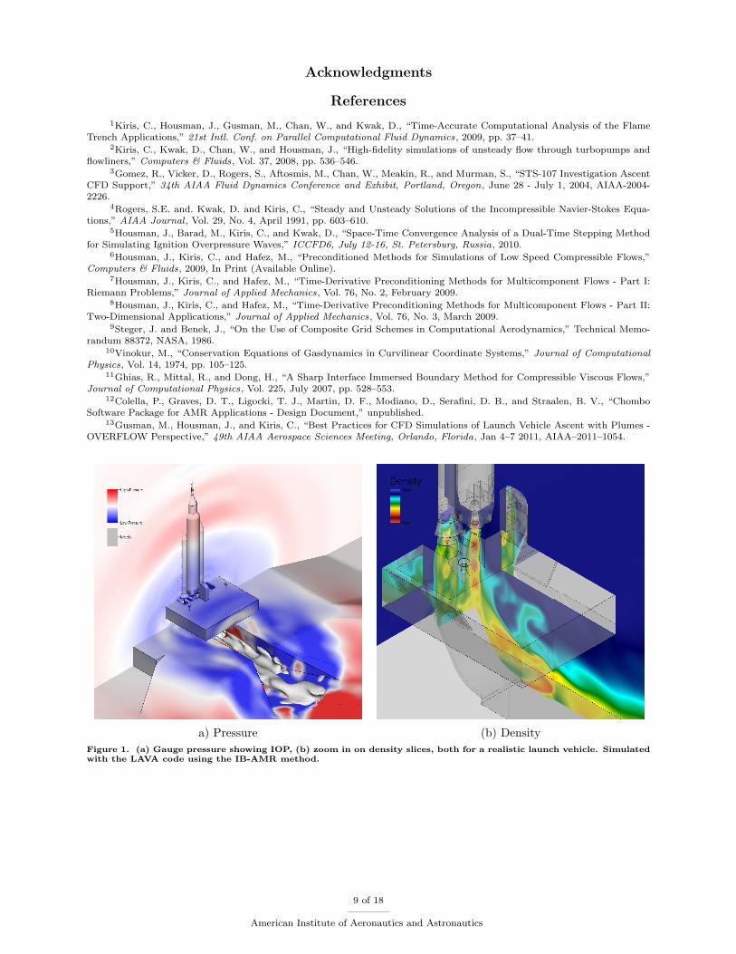
to provide a multi-resolution capability that can coarsen and refine as a simulation progresses. An exampleshowing the 3D IB-AMR capabilities of LAVA for a complex launch environment is shown in Figure 1 and2. These figures illustrate IOP waves generated from Solid Rocket Boosters (SRBs) during the launch ofa HLV. The 3D simulations are computationally expensive, therefore space-time accuracy assessment areperformed on 2D representative problems to determine resolution requirements.

III. Results and Analysis

III.A. Ignition Overpressure Problem

The IOP model problem was jointly defined by NASA and the Japan Aerospace Exploration Agency (JAXA)through a collaborative agreement. The geometry for the IOP wave propagation problem consists of a 2Drocket nozzle located above a 45-degree flat plate, as shown in Figure 4(a). The nozzle exit diameter is 0.1meters and is located 0.5 meters above the plate. Unsteady stagnation conditions are prescribed at the nozzleplenum, where the dimensionless stagnation pressure is shown in Figure 4(b) and the stagnation temperatureis held fixed at the reference temperature Tref = 300 K (cold jet). The remaining reference conditions are:pressure Pref = 100 kPa, velocity Uref = 0 m/s, specific heat at constant pressure Cp = 1005 J/kg/K, andthe ratio of specific heats γ = 1.4. Slip-wall boundary conditions are used on the nozzle walls and on theplate for inviscid simulations. The far-field grid is extended away from the region of interest so that theIOP wave never leaves the solution domain within the time integration limits. Fourteen point locations wereselected in the domain of interest, as shown in Figure 4(a), and the time history of pressure at each of theselocations is recorded. Since the purpose of simulating IOP wave phenomenon is to assess the peak pressurevalues (both suction and load), the application dependent functional chosen for the dual time verificationprocedure is the magnitude of the gauge pressure at each selected point location. For each sample point,this functional is mathematically defined as

F (p) = max0≤t≤T

|p(t)− Pref |. (1)

Similar results were obtained at each of the selected point locations, so only the results at point location 6are reported.

Three mesh resolutions were generated for the present analysis. Figures 5(a)–(d) show the entire domain,a diagram of the overlapping grid system, and two different views of the coarse resolution overset grid. Thefinest off-body mesh spacing h for each mesh resolution is chosen to match the outer boundary spacing ofthe near-body grids; h = ∆x = 0.005m (Coarse), h = ∆x/2 (Medium), and h = ∆x/4 (Fine). Table 1displays the number of zones, number of points, and number of CPU cores used for the simulations. Atotal of 10 cases were run on the coarse grid with physical time-steps corresponding to CFL = 0.5, 1,2, 4, ... , 256, and 16 orders of magnitude reduction in the residual at each time-step was required for0 < t < 100 · Dexit/Cref = 0.028796 seconds. A total of five physical time CFLs were chosen from this setand used to perform simulations on the medium and fine grids, in which 16 orders of magnitude reductionin the residual at each time-step was again required. By removing the solution dependence on sub-iterationconvergence criteria, the largest physical time-step which remains accurate to engineering tolerances waschosen for each grid level. In order to reduce computational costs further, the medium mesh with CFL = 4was chosen to perform a sensitivity analysis with respect to convergence criteria. An additional four cases arerun with convergence tolerances of 1, 2, 4, and 8 orders of magnitude residual reduction. This resulted in 24total unsteady cases which required approximately 2 days to complete on NASA Advanced Supercomputing(NAS) Division’s Pleiades supercomputer.

4 of 18


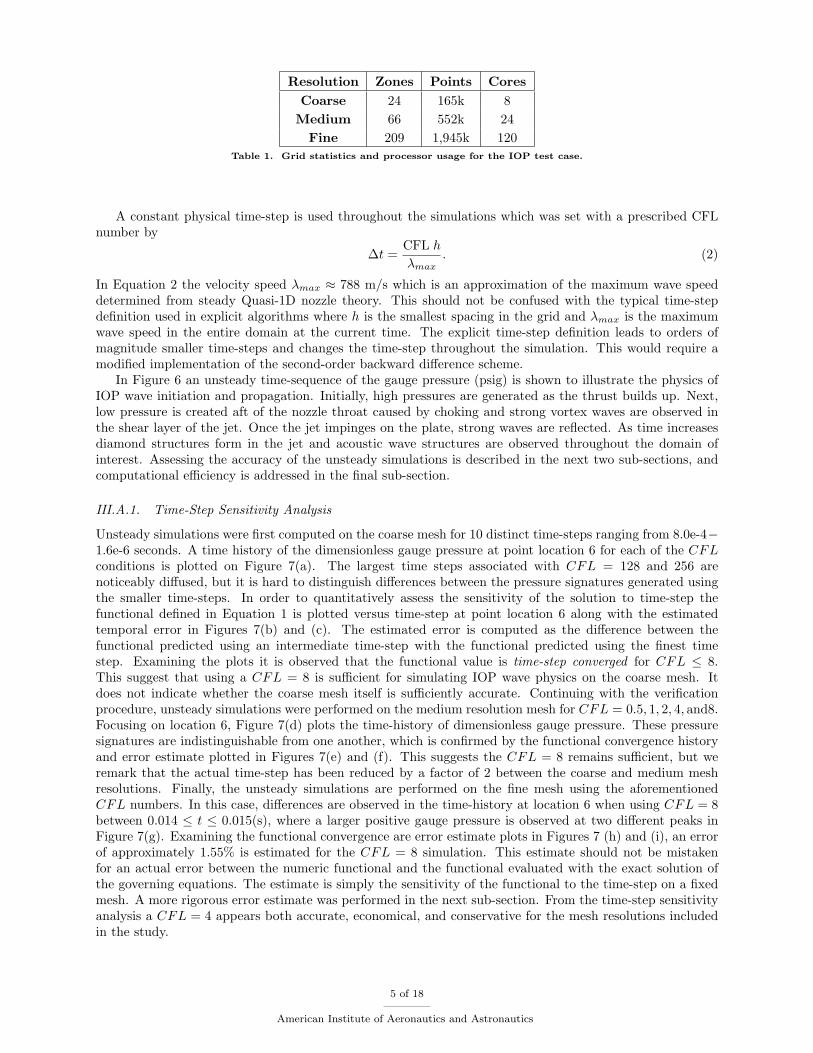
Resolution Zones Points CoresCoarse 24 165k 8Medium 66 552k 24

Fine 209 1,945k 120Table 1. Grid statistics and processor usage for the IOP test case.

A constant physical time-step is used throughout the simulations which was set with a prescribed CFLnumber by

∆t =CFL h

λmax. (2)

In Equation 2 the velocity speed λmax ≈ 788 m/s which is an approximation of the maximum wave speeddetermined from steady Quasi-1D nozzle theory. This should not be confused with the typical time-stepdefinition used in explicit algorithms where h is the smallest spacing in the grid and λmax is the maximumwave speed in the entire domain at the current time. The explicit time-step definition leads to orders ofmagnitude smaller time-steps and changes the time-step throughout the simulation. This would require amodified implementation of the second-order backward difference scheme.

In Figure 6 an unsteady time-sequence of the gauge pressure (psig) is shown to illustrate the physics ofIOP wave initiation and propagation. Initially, high pressures are generated as the thrust builds up. Next,low pressure is created aft of the nozzle throat caused by choking and strong vortex waves are observed inthe shear layer of the jet. Once the jet impinges on the plate, strong waves are reflected. As time increasesdiamond structures form in the jet and acoustic wave structures are observed throughout the domain ofinterest. Assessing the accuracy of the unsteady simulations is described in the next two sub-sections, andcomputational efficiency is addressed in the final sub-section.

III.A.1. Time-Step Sensitivity Analysis

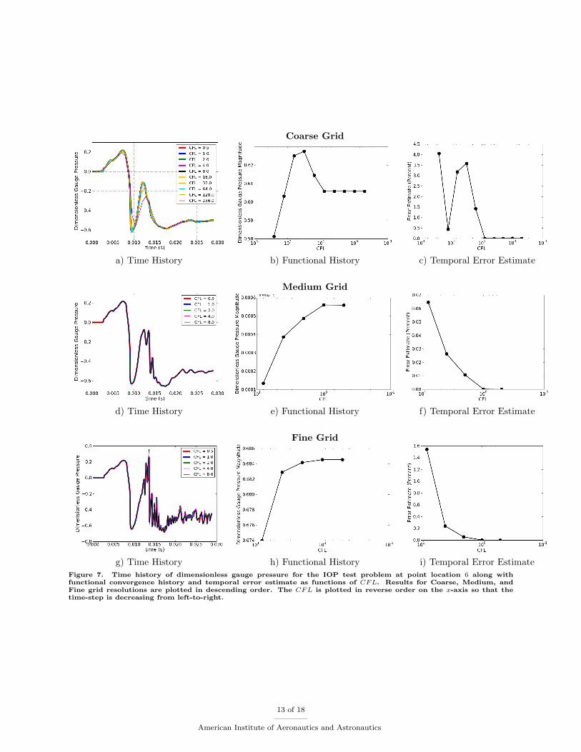
Unsteady simulations were first computed on the coarse mesh for 10 distinct time-steps ranging from 8.0e-4−1.6e-6 seconds. A time history of the dimensionless gauge pressure at point location 6 for each of the CFLconditions is plotted on Figure 7(a). The largest time steps associated with CFL = 128 and 256 arenoticeably diffused, but it is hard to distinguish differences between the pressure signatures generated usingthe smaller time-steps. In order to quantitatively assess the sensitivity of the solution to time-step thefunctional defined in Equation 1 is plotted versus time-step at point location 6 along with the estimatedtemporal error in Figures 7(b) and (c). The estimated error is computed as the difference between thefunctional predicted using an intermediate time-step with the functional predicted using the finest timestep. Examining the plots it is observed that the functional value is time-step converged for CFL ≤ 8.This suggest that using a CFL = 8 is sufficient for simulating IOP wave physics on the coarse mesh. Itdoes not indicate whether the coarse mesh itself is sufficiently accurate. Continuing with the verificationprocedure, unsteady simulations were performed on the medium resolution mesh for CFL = 0.5, 1, 2, 4, and8.Focusing on location 6, Figure 7(d) plots the time-history of dimensionless gauge pressure. These pressuresignatures are indistinguishable from one another, which is confirmed by the functional convergence historyand error estimate plotted in Figures 7(e) and (f). This suggests the CFL = 8 remains sufficient, but weremark that the actual time-step has been reduced by a factor of 2 between the coarse and medium meshresolutions. Finally, the unsteady simulations are performed on the fine mesh using the aforementionedCFL numbers. In this case, differences are observed in the time-history at location 6 when using CFL = 8between 0.014 ≤ t ≤ 0.015(s), where a larger positive gauge pressure is observed at two different peaks inFigure 7(g). Examining the functional convergence are error estimate plots in Figures 7 (h) and (i), an errorof approximately 1.55% is estimated for the CFL = 8 simulation. This estimate should not be mistakenfor an actual error between the numeric functional and the functional evaluated with the exact solution ofthe governing equations. The estimate is simply the sensitivity of the functional to the time-step on a fixedmesh. A more rigorous error estimate was performed in the next sub-section. From the time-step sensitivityanalysis a CFL = 4 appears both accurate, economical, and conservative for the mesh resolutions includedin the study.

5 of 18


III.A.2. Space-Time Sensitivity Analysis

The second step of the dual time verification procedure is to analyze the sensitivity to space-time resolution.From the results of the time-step sensitivity analysis the unsteady solution computed on each mesh levelwith a time-step associated with CFL = 4 are used to perform the space-time sensitivity analysis. Figure8(a) plots the time history of dimensionless gauge pressure at location 6 for each mesh level. It is observedthat higher frequency wave content is captured as the spatial and temporal resolution increases. Second,the suction pressure appears to have two peaks that are very close in magnitude. The first peak appearssmooth and well-resolved on each mesh, while the second peak appears after the onset of small scale acousticeffects. This might have affected the space-time functional convergence if finer grids are included in thestudy. The space-time functional convergence is analyzed in Figures 8(b) and (c) which plots the functionalvalue versus mesh size h along with a log-log plot of the difference between the functional predicted on thecoarse and medium meshes with the fine mesh. The difficulty in achieving true space-time convergence isevident, the functional values are clearly increasing with finer mesh resolution. With that said, the percenterror between the functional values predicted on the fine and medium meshes is below 5% (the black dashedhorizontal line) which is a reasonable engineering tolerance for such complicated physical phenomenon. It isalso observed that the error is reducing at almost second-order (blue dashed line is second order slope whilered dashed line is first-order). This is promising considering the highly nonlinear nature of the flow whichincludes many shock waves and contact discontinuities. Overall the medium mesh resolution with CFL = 4appears to be an adequate choice for simulating IOP waves.

III.A.3. Convergence Tolerance Analysis

The dual time verification procedure, consisting of time-step and space-time sensitivity analyses, has providedquantitative evidence indicating sufficient spatial and temporal resolution requirements for modeling IOPwaves. In the previous analysis the coupled nonlinear system of equations were solved at each time-step usinga 16-order of magnitude residual reduction criteria. This is very severe, and not necessary for maintainingthe solution accuracy. In order to determine a more economical convergence criteria, while maintainingthe accuracy of the simulation, a convergence tolerance study is performed. The unsteady simulation iscomputed using the medium mesh and CFL = 4 with residual reduction tolerances of 1, 2, 4, and 8 ordersof magnitude. The time history and functional sensitivity to convergence tolerance are used to assess theaccuracy of the simulations. In this study the error estimated using the functional value predicted using the16-orders of magnitude residual reduction results previously computed. Large phase and amplitude errorsare observed in the time history plot, shown in Figure 9(a), when the nonlinear residual is only convergedone to two orders of magnitude at each time-step. Examining the functional convergence and error estimateplots in Figure 9(b) and (c), four orders of magnitude convergence in residual appears sufficient to maintainan engineering level accuracy.

III.B. Launch Acoustic Problem

III.B.1. Problem Setup

After determining relevant spatial and temporal resolution requirements for simulating IOP wave phe-nomenon, a similar dual time verification procedure was applied to a model launch acoustic problem. Thelaunch acoustic model problem was designed to assess the capability of the dual-time stepping method incapturing noise generation and sound propagation. The geometry of the problem consists of a fictitiousaxisymmetric launch site containing a generic rocket, mobile launcher (ML), and flame trench as shown inFigure 10(a). This domain is represented using a single-plane and axisymmetric source terms are includedin the governing system of equations. Twenty-seven point locations were selected for recording the unsteadypressure history, which are shown in 10(b). Identical reference conditions as those described above are usedfor this case. The interior of the nozzle is not modeled, and a steady supersonic nozzle exit profile is imposedon the nozzle exit, see Reference13 for details. As in the previous case, slip-walls are used for the rocket,mobile launcher, and flame trench. The far-field is also extended far away from the rocket and extremelycoarse meshes are used in the far-field to sufficiently dissipate the pressure waves before they reach gridboundaries, avoiding spurious reflections.

Four mesh resolutions were generated for the launch acoustic problem, and a diagram of the overlappinggrid system is shown in the upper right corner of Figure 10(a). The finest off-body mesh spacing h for each

6 of 18


grid resolution (again chosen to match the outer boundary spacing of the near-body grids) and the timesteps used for the CFD runs were:

• Coarse: h = ∆x = 0.15m and eight time steps ranging from 3.20×10−4 ≤ ∆t ≤ 2.50×10−6 seconds.

• Medium: h = ∆x/2 and eight time steps ranging from 8.00× 10−5 ≤ ∆t ≤ 6.25× 10−7 seconds.

• Fine: h = ∆x/4 and seven time steps ranging from 4.00× 10−5 ≤ ∆t ≤ 6.25× 10−7 seconds.

• Ultra-Fine: h = ∆x/8 and six time steps ranging from 2.00× 10−5 ≤ ∆t ≤ 6.25× 10−7 seconds.

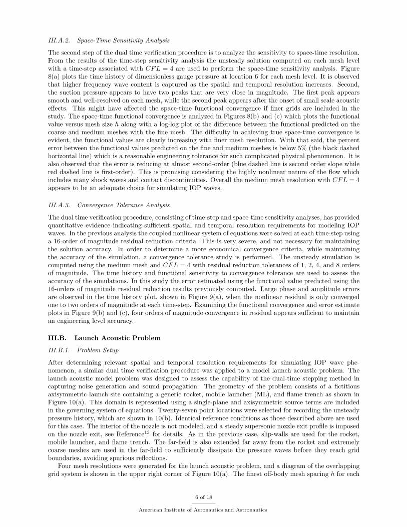
Dimensional time-steps are listed above, instead of the CFLs used in the previous analysis. Each case wassimulated for one second of physical time with a convergence criteria of 16 orders of magnitude reductionin the global L2 norm of the residual at each physical time-step. This eliminated incomplete sub-iterationconvergence from the analysis, as was done for the IOP problem. Table 2 displays the number of zones,number of points, and number of CPU cores used for the overset method.

Resolution Zones Points CoresCoarse 59 171k 8Medium 102 503k 24

Fine 247 1,603k 84Ultra-Fine 674 5,484k 264

Table 2. Grid statistics and processor usage for the launch acoustic test case.

A time sequence of the gauge pressure showing the initiation and propagation of the launch acousticsis displayed in Figure 11. For the acoustic simulations the rocket is held stationary at 60.96 m. abovethe mobile launcher. Since the time scale of the launch acoustics is much smaller than the time it takes arocket to travel away from the launch facility, this assumption should be valid (at least over some specifictime interval). Before the acoustic behavior of the flow field is considered, the initial transient pressurewaves must pass out of the domain of interest. This initial wave is seen in the first two images of thesequence, (t = 0.256 and 0.512 s). Once the initial transient has subsided, the jet impinging on the trenchand interacting with the mobile launcher creates a phenomenon called Duct Overpressure (DOP). The DOPwaves travel back up the hole of the mobile launcher and out of the sides between the launcher and the flametrench, (t = 0.768 and 1.000 s). Along with the DOP waves, the jet creates lower amplitude sound waves,known as Mach waves, which interact with the DOP waves and the launch structure. These simulations areintended to capture the generation, reflection, and interaction of the acoustic waves, all within an idealizedaxisymmetric simulation in order to assess the resolution requirements for 3D simulations.

In order to apply the dual time verification procedure and quantify the accuracy of the launch acousticsimulations, a functional associated with sound pressure level is used. In this case, the Root-Mean-Squared(RMS) functional of gauge pressure is chosen as the application dependant functional,

FRMS(p) =

[1

(T2 − T1)

∫ T2

T1

(p(t)− Pref )2 dt

] 12

. (3)

The two time instances used in the functional are, T1 = 0 and T2 = 1.0. Although this time interval is toshort for extracting relevant sound pressure levels, acoustic effects appear to dominate the pressure signatureafter 0.5 seconds.

III.B.2. Time-Step Sensitivity Analysis

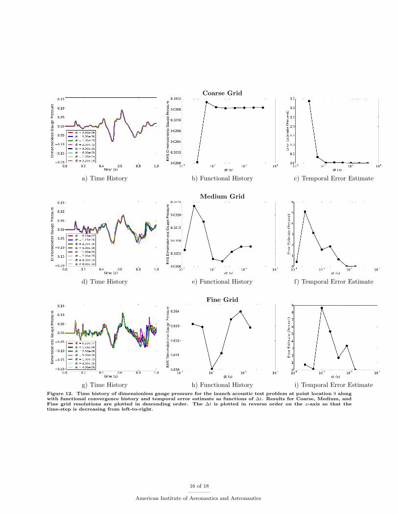
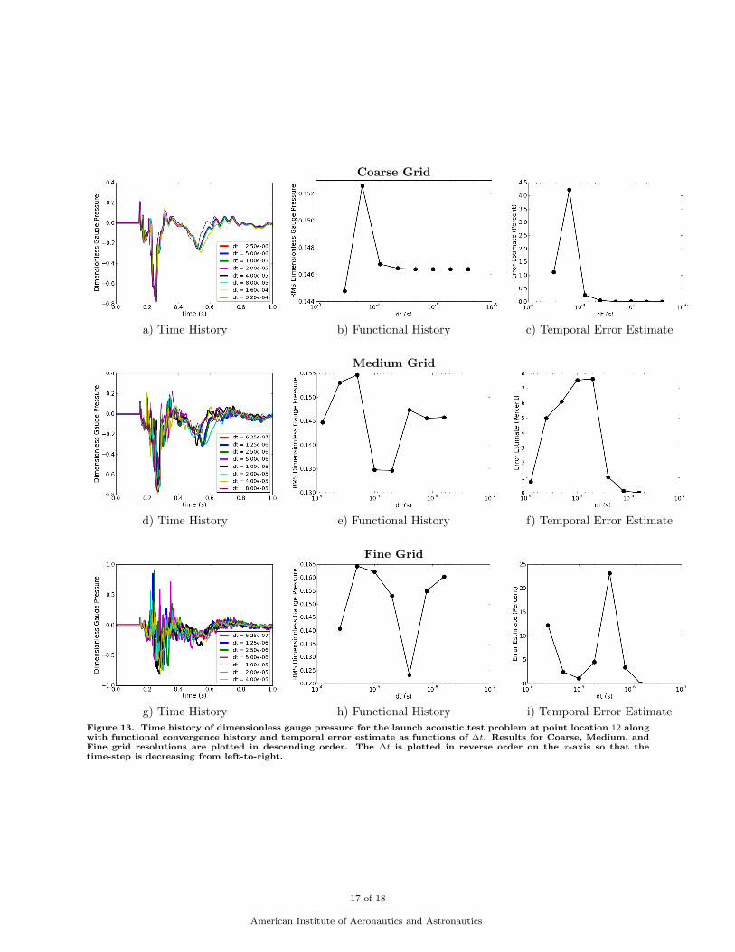
The axisymmetric launch acoustic test case analysis was more computationally expensive than the IOP testcase due to the longer time integration and the additional mesh resolution. The computational cost theultra-fine mesh resolution and smallest time-step was approximately 10 days of continuous runtime using264 cores. Results from this study are shown for point locations 9 and 12 which are located on the payloadsection of the generic rocket and on the bottom corner (jet side) of the ML, see Figure 10. Figure 12(a)–(i)shows the time history of dimensionless gauge pressure, the functional convergence history, and the temporal

7 of 18


error estimates for the coarse, medium and fine mesh resolutions at point location 9. As the spatial resolutionincreases, higher frequency wave content is captured (though under-resolved) as expected from the broadbandnature of launch acoustics. The qualitative features such as the larger IOP and DOP waves appear to becaptured, but larger variations in the small amplitude waves are observed as the mesh and time-step arerefined. Examining the functional history and temporal error estimates, time-step convergence is achievedon the coarse and medium mesh resolutions, but not on the fine mesh resolution. The same observations aremade at point location 12 where Figure 13(a)–(i) shows the time history of dimensionless gauge pressure,the functional convergence history, and the temporal error estimates for the coarse, medium and fine meshresolutions. Comparing the time and functional histories, it appears that point location 9 contains less highfrequency wave content in the pressure history and is better behaved with respect to percent error withdecreasing time-step. This makes sense since location 9 is in a region where acoustic waves are propagatedto, while location 12 is in a noise generating region of the domain. This distinction of how well the currentCFD tools predict noise generating and acoustic propagation regions will be elaborated in the next section.Overall it appears that time-step convergence is difficult to achieve for the launch acoustic problem as themesh is refined.

III.B.3. Space-Time Sensitivity Analysis

Once the initial 23 unsteady simulations were completed for the coarse, medium, and fine grids and thetime-step sensitivity analysis was performed, an additional ultra-fine grid was generated and 6 unsteadysimulations were performed in order to assess the space-time sensitivity of the RMS functional for the launchacoustic problem. From these results the fixed ratio ∆t/∆x = 1/15260 is chosen and the time history,functional history, and space-time error estimate for point locations 9 and 12 are compared in Figures 14(a)–(f). The time-histories plotted in Figures 14(a) and (d) show that additional high frequency information iscaptured at both point locations as the resolution is increased in both space and time. Phase differences arealso evident at location 9 after 0.4 seconds. Similar to the IOP results of the space-time sensitivity analysisthe functional history at location 9 appears to be trending toward a converged value, but is not convergedin space-time. The functional history at location 12 is much worse, showing no sign of convergence in space-time. In fact the error estimate appears to be increasing with resolution. This analysis suggests that noisegenerating regions may be too energetic to converge using the present definition. It may be necessary toredefine the functional such that only certain frequencies in time are included in the RMS functional. Ingeneral it does not appear that the dual time stepping method with second-order (space and time) upwindschemes are capable of achieving space-time convergence nor engineering level accuracy for launch acousticproblems throughout the domain. These methods may be used in conjunction with linearized aeroacoustictools in a hybrid fashion, which is one of the paths of future work the authors are examining. Alternatively,higher-order and/or adaptive methods may be promising.

IV. Conclusion

A dual-time stepping method has been applied to two launch environment test cases. A large parameterstudy was presented examining the sensitivity of unsteady pressure history to time-step and mesh size. A dualtime verification procedure was developed to assess the accuracy of the simulations (since no experimentalor flight data exists for these cases). Time-step convergence on a fixed mesh was demonstrated for the IOPwave problem and on the coarse and medium mesh of the launch acoustic problem. Space-time convergenceanalysis was performed and the selected functionals do not appear to be converged indicating that additionalrefinement (much finer than practical for 3D simulations) is required. Space-time error estimates below5% tolerance level are achieved for the IOP problem but not the launch acoustic problem. Study of thespace-time convergence properties of the dual-time stepping method applied to launch environment flowsis ongoing. Pure CFD analysis for launch acoustic flows is expensive and under-resolved. Future efforts inmodeling launch acoustics will focus on investigating hybrid approaches using empirical information, analyticmethods, and computational aeroacoustic analysis (CAA) in conjunction with CFD results.

8 of 18


Acknowledgments

References

1Kiris, C., Housman, J., Gusman, M., Chan, W., and Kwak, D., “Time-Accurate Computational Analysis of the FlameTrench Applications,” 21st Intl. Conf. on Parallel Computational Fluid Dynamics, 2009, pp. 37–41.

2Kiris, C., Kwak, D., Chan, W., and Housman, J., “High-fidelity simulations of unsteady flow through turbopumps andflowliners,” Computers & Fluids, Vol. 37, 2008, pp. 536–546.

3Gomez, R., Vicker, D., Rogers, S., Aftosmis, M., Chan, W., Meakin, R., and Murman, S., “STS-107 Investigation AscentCFD Support,” 34th AIAA Fluid Dynamics Conference and Exhibit, Portland, Oregon, June 28 - July 1, 2004, AIAA-2004-2226.

4Rogers, S.E. and. Kwak, D. and Kiris, C., “Steady and Unsteady Solutions of the Incompressible Navier-Stokes Equa-tions,” AIAA Journal , Vol. 29, No. 4, April 1991, pp. 603–610.

5Housman, J., Barad, M., Kiris, C., and Kwak, D., “Space-Time Convergence Analysis of a Dual-Time Stepping Methodfor Simulating Ignition Overpressure Waves,” ICCFD6, July 12-16, St. Petersburg, Russia, 2010.

6Housman, J., Kiris, C., and Hafez, M., “Preconditioned Methods for Simulations of Low Speed Compressible Flows,”Computers & Fluids, 2009, In Print (Available Online).

7Housman, J., Kiris, C., and Hafez, M., “Time-Derivative Preconditioning Methods for Multicomponent Flows - Part I:Riemann Problems,” Journal of Applied Mechanics, Vol. 76, No. 2, February 2009.

8Housman, J., Kiris, C., and Hafez, M., “Time-Derivative Preconditioning Methods for Multicomponent Flows - Part II:Two-Dimensional Applications,” Journal of Applied Mechanics, Vol. 76, No. 3, March 2009.

9Steger, J. and Benek, J., “On the Use of Composite Grid Schemes in Computational Aerodynamics,” Technical Memo-randum 88372, NASA, 1986.

10Vinokur, M., “Conservation Equations of Gasdynamics in Curvilinear Coordinate Systems,” Journal of ComputationalPhysics, Vol. 14, 1974, pp. 105–125.

11Ghias, R., Mittal, R., and Dong, H., “A Sharp Interface Immersed Boundary Method for Compressible Viscous Flows,”Journal of Computational Physics, Vol. 225, July 2007, pp. 528–553.

12Colella, P., Graves, D. T., Ligocki, T. J., Martin, D. F., Modiano, D., Serafini, D. B., and Straalen, B. V., “ChomboSoftware Package for AMR Applications - Design Document,” unpublished.

13Gusman, M., Housman, J., and Kiris, C., “Best Practices for CFD Simulations of Launch Vehicle Ascent with Plumes -OVERFLOW Perspective,” 49th AIAA Aerospace Sciences Meeting, Orlando, Florida, Jan 4–7 2011, AIAA–2011–1054.

a) Pressure (b) DensityFigure 1. (a) Gauge pressure showing IOP, (b) zoom in on density slices, both for a realistic launch vehicle. Simulatedwith the LAVA code using the IB-AMR method.

9 of 18


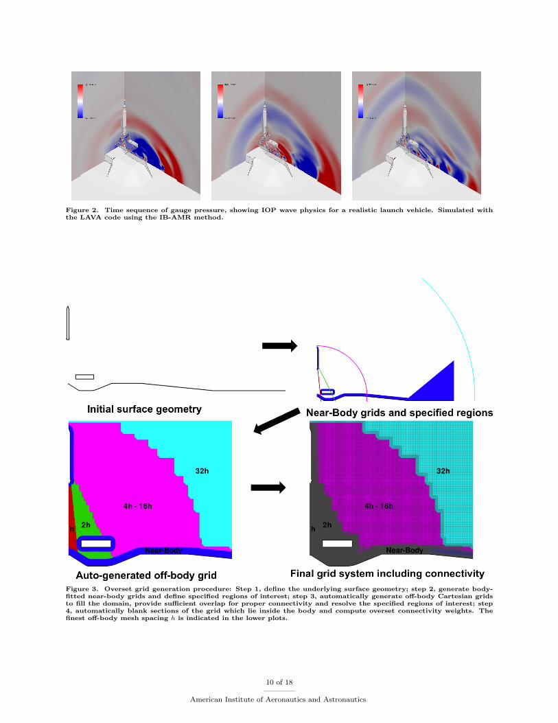
Figure 2. Time sequence of gauge pressure, showing IOP wave physics for a realistic launch vehicle. Simulated withthe LAVA code using the IB-AMR method.

Figure 3. Overset grid generation procedure: Step 1, define the underlying surface geometry; step 2, generate body-fitted near-body grids and define specified regions of interest; step 3, automatically generate off-body Cartesian gridsto fill the domain, provide sufficient overlap for proper connectivity and resolve the specified regions of interest; step4, automatically blank sections of the grid which lie inside the body and compute overset connectivity weights. Thefinest off-body mesh spacing h is indicated in the lower plots.

10 of 18


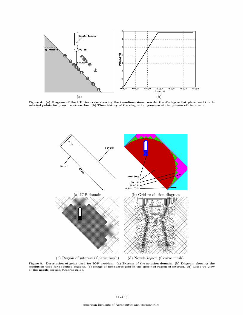
(a) (b)Figure 4. (a) Diagram of the IOP test case showing the two-dimensional nozzle, the 45-degree flat plate, and the 14selected points for pressure extraction. (b) Time history of the stagnation pressure at the plenum of the nozzle.

(a) IOP domain (b) Grid resolution diagram

(c) Region of interest (Coarse mesh) (d) Nozzle region (Coarse mesh)Figure 5. Description of grids used for IOP problem. (a) Extents of the solution domain. (b) Diagram showing theresolution used for specified regions. (c) Image of the coarse grid in the specified region of interest. (d) Close-up viewof the nozzle section (Coarse grid).

11 of 18


t = 0.0036 (s) t = 0.0072 (s) t = 0.0108 (s)

t = 0.0144 t = 0.0180 (s) t = 0.0216 (s)Figure 6. Time sequence of gauge pressure (psig) showing the IOP wave physics, the X- and Y-axis labels are in meters.

12 of 18


Coarse Grid

a) Time History b) Functional History c) Temporal Error Estimate

Medium Grid

d) Time History e) Functional History f) Temporal Error Estimate

Fine Grid

g) Time History h) Functional History i) Temporal Error EstimateFigure 7. Time history of dimensionless gauge pressure for the IOP test problem at point location 6 along withfunctional convergence history and temporal error estimate as functions of CFL. Results for Coarse, Medium, andFine grid resolutions are plotted in descending order. The CFL is plotted in reverse order on the x-axis so that thetime-step is decreasing from left-to-right.

13 of 18


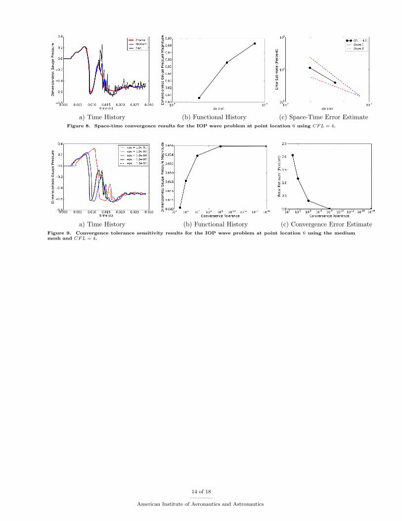
a) Time History (b) Functional History (c) Space-Time Error EstimateFigure 8. Space-time convergence results for the IOP wave problem at point location 6 using CFL = 4.

a) Time History (b) Functional History (c) Convergence Error EstimateFigure 9. Convergence tolerance sensitivity results for the IOP wave problem at point location 6 using the mediummesh and CFL = 4.

14 of 18


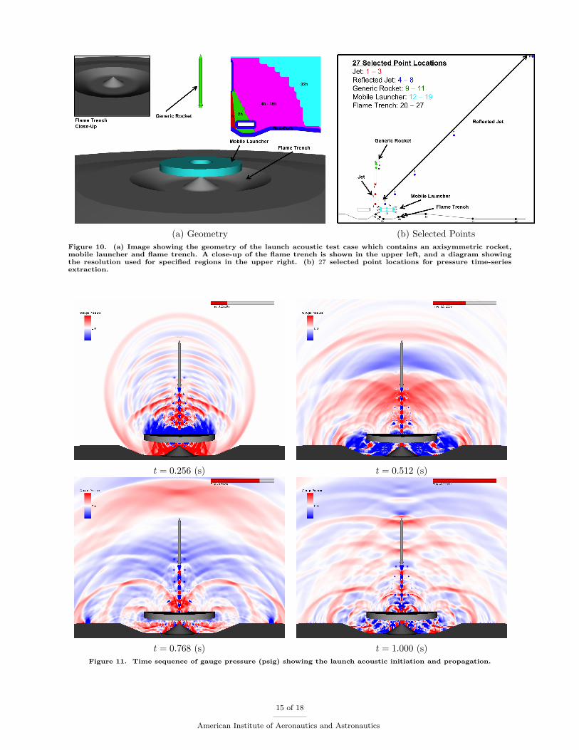
(a) Geometry (b) Selected PointsFigure 10. (a) Image showing the geometry of the launch acoustic test case which contains an axisymmetric rocket,mobile launcher and flame trench. A close-up of the flame trench is shown in the upper left, and a diagram showingthe resolution used for specified regions in the upper right. (b) 27 selected point locations for pressure time-seriesextraction.

t = 0.256 (s) t = 0.512 (s)

t = 0.768 (s) t = 1.000 (s)Figure 11. Time sequence of gauge pressure (psig) showing the launch acoustic initiation and propagation.

15 of 18


Coarse Grid


Medium Grid


Fine Grid

g) Time History h) Functional History i) Temporal Error EstimateFigure 12. Time history of dimensionless gauge pressure for the launch acoustic test problem at point location 9 alongwith functional convergence history and temporal error estimate as functions of ∆t. Results for Coarse, Medium, andFine grid resolutions are plotted in descending order. The ∆t is plotted in reverse order on the x-axis so that thetime-step is decreasing from left-to-right.

16 of 18


Coarse Grid


Medium Grid


Fine Grid

g) Time History h) Functional History i) Temporal Error EstimateFigure 13. Time history of dimensionless gauge pressure for the launch acoustic test problem at point location 12 alongwith functional convergence history and temporal error estimate as functions of ∆t. Results for Coarse, Medium, andFine grid resolutions are plotted in descending order. The ∆t is plotted in reverse order on the x-axis so that thetime-step is decreasing from left-to-right.

17 of 18


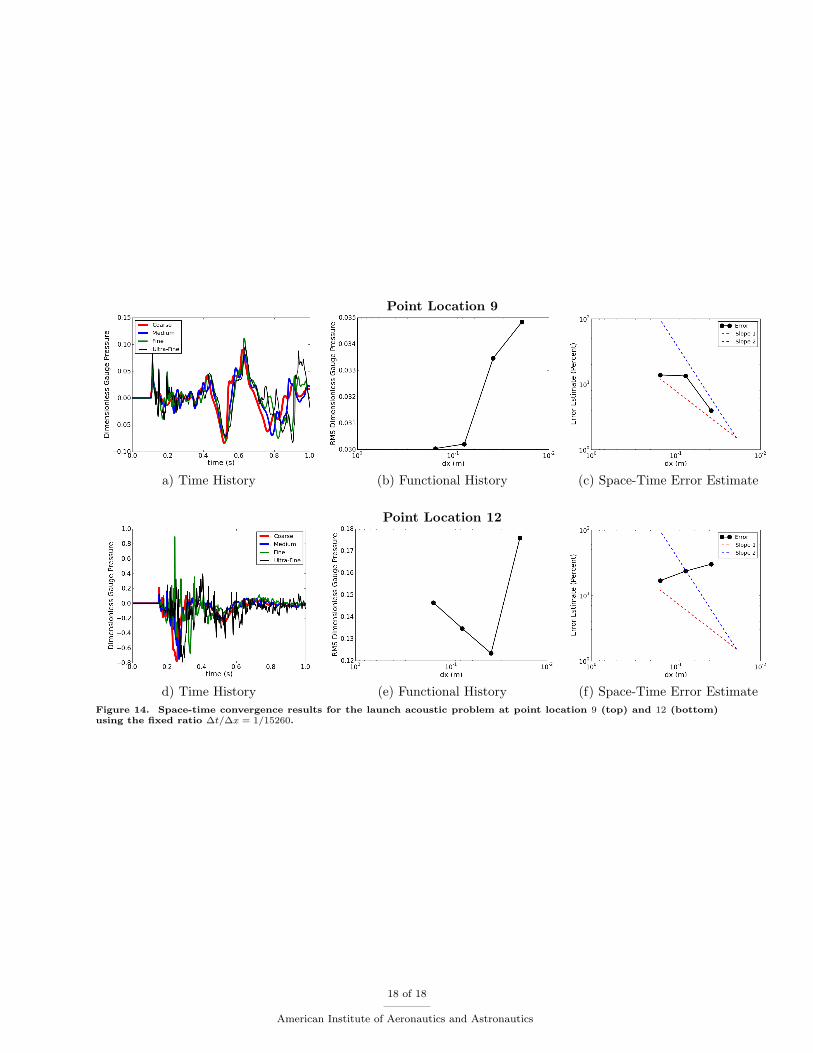
Point Location 9

a) Time History (b) Functional History (c) Space-Time Error Estimate

Point Location 12

d) Time History (e) Functional History (f) Space-Time Error EstimateFigure 14. Space-time convergence results for the launch acoustic problem at point location 9 (top) and 12 (bottom)using the fixed ratio ∆t/∆x = 1/15260.

18 of 18


Documents

Space Time Accuracy Assessment of CFD Simulations for the ... · Space-Time Accuracy Assessment of CFD Simulations for the Launch Environment Jeﬀrey A. Housman∗ and Michael F