CFD Simulations of the Space Launch System Ascent

CFD Simulations of the Space Launch SystemAscent Aerodynamics and Booster Separation

Stuart E. Rogers∗

NASA Ames Research Center, Moffett Field, CA 94035, USA

Derek J. Dalle†

Science and Technology Corp., Moffett Field, CA 94035, USA

William M. Chan‡

NASA Ames Research Center, Moffett Field, CA 94035, USA

This paper presents details of Computational Fluid Dynamic modeling of the Space LaunchSystem during ascent. The primary focus of the paper is the flow simulation of the vehi-cle during ascent using the Overflow Navier-Stokes code. Computations of 739 first-stageflight conditions covering a range of Mach numbers, angles of attack, and roll angles werecomputed. The overset grid system contained 375 million grid points, and over 28 mil-lion CPU hours were used in the simulations. The simulations were run on the Pleiadessupercomputer at the NASA Advanced Supercomputer Center at Ames Research Center.The data products from this work include integrated line-loads, surface pressure coeffi-cients, venting pressures, and protuberance air-loads. Detailed comparisons were made ofthe aerodynamic performance predicted by Overflow and the wind-tunnel derived aero-dynamic database. A small number of the cases were run with two different turbulencemodels and with two differencing schemes. These results were used to quantify the sensi-tivity to the choice of the turbulence model and to the differencing scheme. The paper alsointroduces an effort to use the inviscid, unstructured Cartesian solver Cart3D to computethe aerodynamics during booster separation. Adaptive mesh refinement is being used toenable accurate simulations of sixteen booster-separation-motor plumes. The use of thistool is explored in preparation for building a booster-separation aerodynamic database.

I. IntroductionThe NASA Space Launch System (SLS) will provide an entirely new heavy-lift capability that enableslaunch of more mass to orbit than any other launch vehicle, and makes possible crew missions beyondEarth orbit. The initial SLS configuration, shown in Fig. 1, consists of a 200-foot core stage, right and leftsolid-rocket boosters, an interim cryogenic propulsion stage, stage adapter, and the Orion spacecraft. Thisconfiguration has a 70-metric ton payload capability, will provide 10 percent more thrust at launch than theSaturn V rocket, and carry more than three times the payload of the space shuttle.

The SLS program is tasked with developing an all new series of launch vehicles, and although manycomponents include legacy hardware from the Space Shuttle program, this requires developing many aero-dynamic related databases. Budget limitations constrain the number of wind-tunnel tests, thus the programrelies on Computational Fluid Dynamics (CFD) analysis to provide a significant amount of data. Use ofCFD enables a reduction in conservatism that can be translated into higher payload to orbit.

Recent CFD analysis of launch vehicle ascent aerodynamics included work for the NASA Space Shuttleprogram. This work included aerodynamic analysis of the events leading to the Columbia accident during theSTS-107 mission [1], CFD analysis used in debris-transport analysis [2], aerodynamic analysis of proposed

∗Aerospace Eng., NASA Advanced Supercomputing Division, Associate Fellow AIAA, [email protected]†Research Scientist/Engineer, NASA Advanced Supercomputing Division, Member AIAA, [email protected]‡Computer Scientist, NASA Advanced Supercomputing Division, Senior Member AIAA, [email protected]

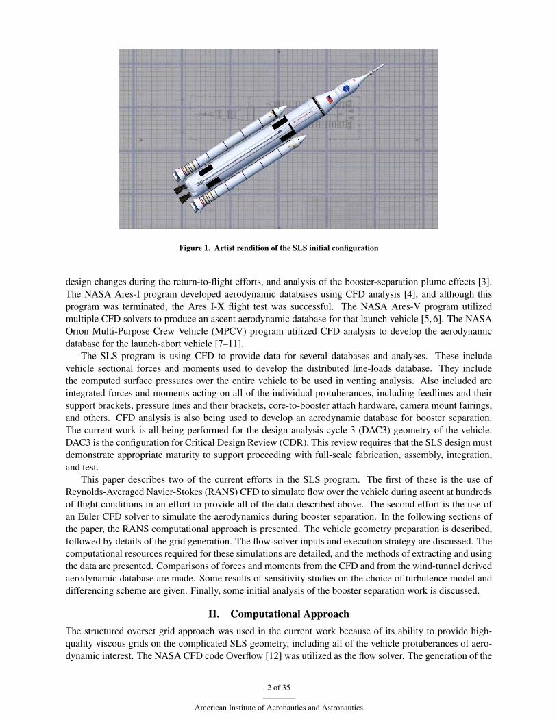
Figure 1. Artist rendition of the SLS initial configuration

design changes during the return-to-flight efforts, and analysis of the booster-separation plume effects [3].The NASA Ares-I program developed aerodynamic databases using CFD analysis [4], and although thisprogram was terminated, the Ares I-X flight test was successful. The NASA Ares-V program utilizedmultiple CFD solvers to produce an ascent aerodynamic database for that launch vehicle [5, 6]. The NASAOrion Multi-Purpose Crew Vehicle (MPCV) program utilized CFD analysis to develop the aerodynamicdatabase for the launch-abort vehicle [7–11].

The SLS program is using CFD to provide data for several databases and analyses. These includevehicle sectional forces and moments used to develop the distributed line-loads database. They includethe computed surface pressures over the entire vehicle to be used in venting analysis. Also included areintegrated forces and moments acting on all of the individual protuberances, including feedlines and theirsupport brackets, pressure lines and their brackets, core-to-booster attach hardware, camera mount fairings,and others. CFD analysis is also being used to develop an aerodynamic database for booster separation.The current work is all being performed for the design-analysis cycle 3 (DAC3) geometry of the vehicle.DAC3 is the configuration for Critical Design Review (CDR). This review requires that the SLS design mustdemonstrate appropriate maturity to support proceeding with full-scale fabrication, assembly, integration,and test.

This paper describes two of the current efforts in the SLS program. The first of these is the use ofReynolds-Averaged Navier-Stokes (RANS) CFD to simulate flow over the vehicle during ascent at hundredsof flight conditions in an effort to provide all of the data described above. The second effort is the use ofan Euler CFD solver to simulate the aerodynamics during booster separation. In the following sections ofthe paper, the RANS computational approach is presented. The vehicle geometry preparation is described,followed by details of the grid generation. The flow-solver inputs and execution strategy are discussed. Thecomputational resources required for these simulations are detailed, and the methods of extracting and usingthe data are presented. Comparisons of forces and moments from the CFD and from the wind-tunnel derivedaerodynamic database are made. Some results of sensitivity studies on the choice of turbulence model anddifferencing scheme are given. Finally, some initial analysis of the booster separation work is discussed.

II. Computational ApproachThe structured overset grid approach was used in the current work because of its ability to provide high-quality viscous grids on the complicated SLS geometry, including all of the vehicle protuberances of aero-dynamic interest. The NASA CFD code Overflow [12] was utilized as the flow solver. The generation of the

2 of 35

American Institute of Aeronautics and Astronautics

overset grids is time-intensive and requires significant user expertise compared to production unstructuredCFD flow solvers. However, once the grids have been generated, the structured grid approach requires sig-nificantly less computational resources than unstructured solvers. Because the current work requires on theorder of 1000 simulations, the overset-structured grid approach was the only approach capable of producingresults in the required time frame.

The current simulations neglect the effect of the main-engine plumes and the plumes of the solid-rocketboosters. The nozzles were sealed at their exit plane, and the seals were treated as no-slip walls. Thereforethe current surface pressure on the aft end of the vehicle does not include the effects of plumes, or of anyplume-induced flow separation, which only occurs at high altitude just prior to booster separation.

III. Vehicle GeometryThe SLS-10005 outer mold line (OML) geometry served as the basis for the current CFD model. This modelwas simplified further from the original to facilitate the grid-generation process. This was necessary to keepthe total computational requirements within the computational resources available and within the schedulerequirements of the program. The ANSA software was used to manipulate and simplify the geometry, andthen to export the geometry as very fine triangulated surfaces to be used in the surface grid-generationprocess. The primary components of the geometry include the Launch Abort Vehicle (LAV), the MPCVand its service module, the Launch Vehicle Stage Adapter (LVSA), the Core stage, and the two Solid-Rocket Boosters (SRB). Images of the OML geometry details are shown in the following figures. Figure 2ashows the geometry near the LAV abort-motor nozzles, and Fig. 2b shows the geometry of the MPCVboost-protection cover. Figure 2c shows the booster nosecap and forward booster separation motor nozzles.Figure 2d shows the geometry near the forward end of the LO2 feedline and the pressure lines on the corestage, whereas Fig. 2e shows the aft ends of these lines. Figure 2f illustrates the geometry on the aft end ofone of the boosters.

IV. Grid GenerationThe creation of the grid system for the SLS-10005 DAC3 vehicle was a team effort consisting of two experi-enced and two novice users of the grid tools. Taking full advantage of the overset grid approach, grids for thecomponent parts of the complex geometry were generated in parallel by the team members. The axisymmet-ric main component grids (core and boosters) were created first, followed by grids for all the protuberancesthat reside on the main components. Utilizing macros from the Chimera Grid Tools (CGT) [13, 14] version2.1p+ script library, scripts were created for all pre-processing steps needed prior to running the flow solver.These include the generation of surface and volume grids, creation of hole-cutting instructions for oversetdomain connectivity, prescription of boundary conditions in the flow solver input file, and specifications ofcomponents for forces and moments integration. The scripting approach provides a record of the all stepsused in the complex grid generation process, and allows rapid automated re-generation of the entire gridsystem. Key inputs in the grid generation steps such as grid spacings, marching distances and stretchingratios are parameterized in the script. This enables quick grid resolution adjustments to achieve high gridquality.

Surface grids were created using a combination of algebraic and hyperbolic methods via the surgrdmodule in CGT. A maximum surface spacing of ten inches and maximum circumferential resolution of onedegree were utilized in the axisymmetric components. In the vicinity of the attach hardware and protuber-ances, the grids were made to be much finer, and all features were resolved with grid spacings of fractionsof an inch or less. The body-fitted volume grids were generated hyperbolically using the hypgen modulein CGT with a normal viscous wall-spacing targeted to produce the first cell within a Y+ value of 1.0 atmaximum-dynamic pressure conditions. Off-body Cartesian grids were automatically generated using themulti-layer feature in the Overflow flow solver. After combining the individual body-fitted and off-bodygrids, the overset hole-cutting and interpolation were performed using the X-ray capability within CGT andOverflow. The completed grid system was composed of 888 body-fitted zones and 304 Cartesian off-body

3 of 35


a) LAV abort-motor nozzles b) MPCV boost-protection cover

c) Forward booster-separation motors d) Forward end of feedline and pressure lines

e) Aft end of feedline and pressure lines f) Booster aft end

Figure 2. Details of the SLS vehicle geometry.

4 of 35


grids. The total number of grid points was just over 375 million with only 203 orphan points remaining afteroverset connectivity. The entire grid system was created in about two months by the four person team. It isone of the most complex and efficiently generated grid systems using overset structured grids ever produced.Figure 3a shows a side view of the surface and volume grids on the entire vehicle, Fig. 3b shows the surfacegrids on the forward part of the vehicle. Figure 3c shows the surface grids near the nosecap of the rightbooster, and Fig. 3d shows a view of the aft end of the right booster. Figure 3e shows the surface grids on+Z LO2 feedline and brackets, and Fig. 3f shows the surface grids on the forward-attach hardware of theleft booster.

V. Flow ConditionsThe freestream conditions for Mach number (M), total angle of attack (αt), and velocity roll angle (φ) usedin the simulations are:

• M = 0.7, 0.8, 0.9, 0.95, 1.05, 1.10, 1.20, 1.30, 1.40, 1.60, 1.75, 2.0:

– αt = 0.0; φ = 0

– αt = 2.0, 4.0; φ = 0, 30, 45, 60, 90, 120, 135, 150, 180

– αt = 2.0, 4.0; φ = 210, 225, 240, 270, 300, 315, 330

• M = 0.5, 2.5, 3.0, 3.5, 4.0, 4.5, 5.0:

– αt = 0.0; φ = 0

– αt = 2.0, 4.0, 6.0; φ = 30, 45, 60, 90, 120, 135, 150, 180

– αt = 2.0, 4.0, 6.0; φ = 210, 225, 240, 270, 300, 315, 330

VI. Overflow InputsThe flowfields were computed with the standard release version 2.2h of the Overflow code, using theMessage-Passing Interface (MPI) parallel version. The computations were performed on the SGI Altixsystem known as Pleiades at the NASA Advanced Supercomputing (NAS) facility. The computations wereall performed on the Ivy Bridge nodes of this machine. Overflow was compiled using the Intel Fortrancompiler ifort version 2013.5.192 and the SGI MPI implementation mpt.2.10r6. All of the runs used 41 IvyBridge nodes, consisting of 820 cores.

Central differencing plus scalar smoothing was used, in combination with the implicit block tridiagonalapproximate-factorization scheme. All viscous terms, including cross terms, were enabled in the code. TheSpalart-Allmaras turbulence model [15] was used, and the flow was assumed to be turbulent everywhere.These were the baseline Overflow inputs which were used for all of the production cases in the current work.In addition, a small number of cases were run to quantify the sensitivity of the solutions to the choice ofturbulence model and choice of differencing scheme. The sensitivity to the choice of turbulence model wasstudied by repeating some cases using the SST turbulence model [16, 17]. The same set of cases was alsorun using a third-order HLLC upwind-differencing scheme, together with an SSOR line-relaxation implicitscheme.

For the initial start-up phase and for steady-state iterations, first-order time integration was used togetherwith locally-scaled time-step sizes based on a constant Courant-Friedrichs-Lewy (CFL) number. The time-accurate integration used a dual time-stepping approach in which the outer-level integration was second-order in time. The inner-level integration used ten sub-iterations per time step with a non-dimensionaltime-step size of 1.0. This corresponds to a physical time-step size of 1.65 × 10−5 to 1.5 × 10−4 seconds forfree-stream Mach numbers ranging from 5.0 to 0.5, respectively. These values were determined after runninga small number of test cases varying both the time-step size and the number of inner sub-iterations. Thiscombination provided reasonably converged results relative to the cost of running more inner sub-iterationsand/or running with a smaller time-step size.

5 of 35


a) Side view of entire grid system b) Forward vehicle surface

c) SRB nosecap d) Booster aft end

e) Liquid oxygen feedline on the core f) Forward attach hardware

Figure 3. Different views of the surface grids on portions of the SLS vehicle.

6 of 35


VII. Overflow Execution and ConvergenceThe following run sequence was found to be the most efficient strategy for the SLS DAC3 calculations.The code was run with a sequence of different inputs, starting with a full-multi-grid sequencing for the first4000 steady-state iterations, using relatively higher dissipation and smaller time-step sizes. Over the next6000 steady-state iterations, the time-step size was increased and the dissipation coefficients were decreasedin three increments. This was followed by 6000 to 10,000 additional steady-state iterations. If the caseconverged to a steady-state, the simulation was terminated. The case was considered converged if the L2-norm of the residual had converged at least three to four orders of magnitude, and the aerodynamic forcecoefficients converged to a steady state. Several different force coefficients were monitored, including theforces acting on the total core, each SRB, large protuberances like the liquid-oxygen feedline, and smallerprotuberances like the aft booster-separation motors on the SRBs.

If the steady-state iterations did not converge or the forces were unsteady, the case was continued withtime-accurate integration. The time-accurate integration was run until the time-averaged mean of the mon-itored force coefficients were converged. Then the final solution was extracted from a time average of thedependent variables over a span of at least 2000 time steps. During the Overflow runs, the code computedthe forces and moments on all components of the vehicle every ten iterations to enable the convergencemonitoring. The moments were all computed about a reference center at the base of the vehicle.

The NASA-developed overlst software was used to execute, manage, and post-process all of the Over-flow runs. This is a script written in the Perl language. The Overflow community has yet to devise a reliableautomatic method for determining convergence, and so the key to implementing this run strategy for hun-dreds of Overflow simulations is the ability to easily monitor the progress of each case. The monitoringwas greatly aided by the use of the overlst software, which greatly simplifies the creation of batches of con-vergence plots which can be easily and rapidly examined by the user. This software also provides a simpleinterface for the user to control batches of simulations, adding more iterations/time-steps, and switchingfrom steady-state to time-accurate integration.

A. Computational Resources

Figure 4 shows a summary of the CPU hours required to run the ascent database simulations, with thecases grouped by Mach number. At each Mach number there are either 14 (from Mach 0.7 to 2.0) or 21(otherwise) αT , φ combinations in the run matrix. The black curve with dots in Fig. 4 shows the averageCPU-hour requirement per case at the given Mach number, and the blue curve is the maximum number ofCPU-hours per case at that Mach number.

Several things stand out in Fig. 4. Most importantly, the cases around Mach 1.0 require the most CPUhours, which is expected since this is the most likely regime for unsteady flow. Second, the CPU require-ments are elevated (compared to those of Mach 5.0) even at true supersonic conditions as high as Mach 3.0.This is because there is not a clean break in Mach number where all lower-Mach cases require time-accuratesolution and all higher-Mach cases are steady. For low supersonic cases, there are often orientations thathave either vortex shedding, unsteady shock interactions, or regions of unsteady flow separation. In fact,the single case requiring the most CPU hours was at Mach 2.5, despite the fact that the average usage atMach 2.5 was quite low. Finally, it is apparent that applying the most conservative run sequence (whichrequired about 85,000 CPU hours) to all cases would dramatically increase the total requirements for theentire run matrix. The total CPU usage for this subset of the run matrix was 3.2 million CPU hours, whereasthe number would have been over 27 million if each case had required 85,000 CPU hours.

The simple piecewise linear curves labeled “planning curves” in Fig. 4 are a simplified interpretationof the data. It was observed that a transonic case takes, on average, about five times as much CPU time asa high supersonic case. Similarly, it was estimated that a worst-case Mach 5.0 case could take as much asthree times more CPU hours than a nominal case, and a worst-case transonic case could take as much as 9times as long as the nominal Mach 5.0 case. If NM5 is the nominal number of CPU hours per case at Mach

7 of 35


Mean CPU usage

Max CPU hours per Mach

Mean CPU planning curve

Max CPU planning curve

Figure 4. CPU usage for ascent database cases grouped by Mach number

5 (in this case 10,000 CPU hours), then the two curves are

N(mean,planning) =

5NM5 : M ≤ 1.1(5 − 5

3 (M − 1.1))NM5 : 1.1 < M ≤ 3.5NM5 : M > 3.5

(1)

N(max,planning) =

9NM5 : M ≤ 2.5(9 − 2.4(M − 2.5))NM5 : 2.5 < M ≤ 5.03NM5 : M > 5.0

(2)

These functions are expected to be valid for most launch vehicle ascent simulations using Overflow, al-though geometry (for example, the presence or absence of large protuberances) can affect the prevalenceof unsteady cases, and significant changes to Overflow inputs will invalidate this calibration. The approach(with additional calibrations to the slopes of the lines, etc.) may also be useful for other types of problemsand other flow solvers, but additional considerations may be relevant. In addition to checking intuition, thesefunctions can be useful for planning, which is discussed in the following subsection.

B. Computational Planning Insights

Typically an estimate of computational resources for a large database such as this one are based on RoughOrder of Magnitude (ROM) analyses that are thought to be conservative. Especially for vehicles or runmatrices outside the experience of the organization completing the analysis, constructing a more accurateBasis Of Estimate (BOE) is difficult or impossible. For example, using a conservative estimate of therequirements at Mach 5.0 may lead to an underestimate of the total requirements for the matrix.

Based on the actual requirements for 315 cases as reported in Fig. 4, a relatively simple planning methodhas been developed where the CPU requirements of a case are a function of the freestream Mach number.First estimate the expected CPU requirements for the nominal inputs, for example by running a single casethrough a set of inputs that is sufficient to converge most high-supersonic cases or using a ROM of the CPUrequirements for a high-supersonic case based on previous experience. Using a high-supersonic case such asMach 5.0 is useful to anchor the estimate even if it is not in the run matrix because the convergence behaviorin this regime is more predictable.

8 of 35


The second step is to generate the “Mean CPU planning curve” as in Fig. 4 based on the estimate forCPU hours at Mach 5.0. This simple function then gives an estimate of the average number of CPU hoursper case as a function of Mach number, fBOE(M), and combining this information with the planned runmatrix leads to an estimate of the total required number of CPU hours.

Mean CPU usage

Mean CPU planning curve

Max CPU planning curve

Figure 5. CPU usage for coarser grid system used for debris transport analysis

Figure 5 shows an example of this procedure applied to the coarser grid system used for debris transportanalysis. Since this system has roughly half as many grid points as the full ascent grid system, a reasonableestimate of the CPU requirements for a Mach 5.0 case is 5000 CPU hours per case (half of the 10,000 forthe full ascent grid system). This is all the information needed to create the “Mean CPU planning curve”and “Max CPU planning curve” in Fig. 5. The run matrix for the debris transport analysis was one conditionat each Mach number marked with a dot in Fig. 5 except for Mach 3.32, at which 13 cases were run. Thenthe total estimate of CPU hours required would be

CPUBOE = fBOE(0.06) + fBOE(0.13) + . . . + fBOE(3.02) + 13 fBOE(3.32) + . . . + fBOE(4.26) (3)

which gives an estimate of 509,000 CPU hours. The actual CPU usage was 483,000 CPU hours, so at leastin this case, the method gave an accurate prediction.

The “Max CPU planning curve” can also be useful in several cases. For one, if the run matrix has onlya small number of conditions, using an average is more likely to underpredict actual CPU requirements, andusing the maximum is a more appropriate conservative estimate. Second, if the computing environment issuch that all or nearly all cases in the run matrix can be executed simultaneously, the worst case in the entirerun matrix provides the best estimate of the wall time required.

When it is not possible to run all or nearly all cases simultaneously, the recommended procedure is tostart with transonic and subsonic cases so that any outliers requiring more time to converge will have achance to do so while running the supersonic cases. This leads to a lower probability of having one or twocases that are still running hours or days after the rest of the run matrix has been completed.

VIII. Data Extraction and DeliveryA. Sectional Loads Data

A key deliverable from the aerodynamics team for structural analysis is the integrated loads on slices ofthe vehicle. That is, the vehicle is first sliced by a number of equally-spaced axial planes, and the forces

9 of 35


and moments on these slices are integrated. The most important components of these loads are the normaland lateral forces, which are the most likely to bend the core stage and two boosters. To calculate theseaerodynamic loads, the following steps are taken.

• The wall and wall-adjacent layers of the solution file are extracted; the second layer is needed tocompute the viscous forces.

• Four sets of cuts are made: one for the core, one for each booster, and one for the entire stack. Eachof these four is cut into 201 slices using the triload program [18] from the CGT package.

• The triload program constructs surface triangles covering each slice.

• Forces and moments are calculated for each slice by integrating the pressure- and viscous-force con-tributions at each triangle.

Figure 6. Legend for plots of sectional loads

Figure 6 is a legend for the example sectional line loads plots shown in Figs. 7 and 8. These figures plotthe sectional loads as a functional of the axial position on the vehicle, scaled by the reference length LREF.The subset of the run matrix used for these examples is a roll sweep at Mach 1.60 with a fixed total angleof attack at 4◦. The sectional loads in Fig. 7 show the expected symmetry: a sign-change in sideslip anglehas little effect on normal forces, and a sign-change in angle of attack (not total angle of attack) has littleeffect on lateral forces. In Fig. 8, the plots are organized such that plots in the same row should be eithersymmetric or anti-symmetric. The normal loads on the left booster (SRBM) at conditions of (α, β) shouldbe similar to the normal loads on the right booster (SRBP) at (α,−β). Unlike the core, there is no symmetryin β because the presence of the core on only one side of the booster means that the sign of β plays a biggerrole. Similarly, the lateral loads on SRBM at (α, β) are close to the opposite of the lateral loads on SRBP at(α,−β).

B. Protuberance Data

Force data on each of the 140 separate protuberances was extracted. These protuberances are essentiallyanything other than the main booster and core bodies; they include parts like attach hardware, cameras,

10 of 35


4 6 8 10 12 14

-1.0

0.0

1.0

a) Normal sectional loads on core

4 6 8 10 12 14

-1.0

0.0

1.0

b) Lateral sectional loads on core

Figure 7. Sectional aerodynamic loads on the core at Mach 1.6 and 4◦ total angle of attack

a) Normal sectional loads on left booster (SRBM) b) Normal sectional loads on right booster (SRBP)

c) Lateral sectional loads on left booster (SRBM) d) Lateral sectional loads on right booster (SRBP)

Figure 8. Sectional aerodynamic loads on the solid rocket boosters at Mach 1.6 and 4◦ total angle of attack

11 of 35


system tunnels, and pressure lines. Extracting the forces on these protuberances is the first step in a processthat ensures that the protuberances remain safely attached and are able to withstand the ascent environment.

The data that is delivered to the protuberance team takes the form of triangulated surface data on eachprotuberance. To obtain this, The mixsur program from CGT is used to create a unique triangulation tocover the surface of each protuberance. Each protuberance is further broken down into individual faces, suchas the top, the bottom, and the sides. A program called overint from the CGT package is used to extractthe surface pressure coefficient (Cp) and force components independently. The final post-processing step isthe conversion of this data into two Tecplot files. One of these files contains the Cp. The other file containsthe three components of the dimensionalized force (broken down into the pressure, viscous, momentum, andtotal contributions) and area on each triangle.

Figure 9 shows an example of axial force extraction on a forward-facing camera on the aft portion of thecore, which is visible in Fig. 2e. The quantity that determines the color is the axial component of force oneach triangle, and thus smaller triangles have less force.

Figure 9. Axial force on each triangle of the core aft camera 1 at Mach 1.2 with αt = 2◦ and φ = 45◦

C. Surface Pressure Data

The surface Cp data on the entire vehicle was extracted and saved as formatted Tecplot data files. Each datafile contains 61 different Tecplot zones corresponding to different components and surfaces on the vehicle.A perl script was used to create the Cp data file for each case. The script uses the overint and the trigedprograms from the CGT package to create a surface triangulation together with the surface Cp data.

D. Boundary Layer Profiles

Boundary layer profiles were extracted to support two independent tasks: venting analysis and scaling buffetforcing functions from wind tunnel data. To extract these boundary layer profiles, the vpro program from

12 of 35


the CGT package was used to extract all state variables along a line segment perpendicular to the surfaceat about 40 locations on the surface. The points at which the boundary layer profiles are extracted are thephysical locations of 33 vents and the locations of several transducers in an unsteady aerodynamics windtunnel test. The data in these boundary layer profiles includes pressure, density, and the three componentsof velocity. The axis for the x-component of the velocity is the projection of the vehicle x-axis into the localtangent plane, the z-component is normal to the surface, and the y-component completes the right-handedsystem. Figure 10 shows the dimensional boundary profiles of the velocity magnitude at one vent locationfor all cases in the run matrix that have zero total angle of attack. there is a tendency for the boundary layerto grow as the freestream pressure decreases and the Reynolds number decreases. The slight kinks seen atthe outer edges of the velocity data is due to the transition in grid resolution as the profiles cross overlappinggrid boundaries.

a) Lower Mach numbers, 0.50 to 1.30 b) Higher Mach numbers, 1.30 to 5.00

Figure 10. Boundary profiles at a vent on the core stage for Mach sweep of conditions at 0◦ total angle of attack

IX. Aerodynamic DataIn this section the integrated force coefficients from the current CFD runs are compared to the aerodynamicdatabook values for the vehicle. The databook values are all based on experimental data, and include un-certainty increments to account for experimental uncertainty and repeatability, and differences between thewind-tunnel results and the flight vehicle. The Overflow CFD data in the following figures excludes thebase region of the core to best match the experimental model, whose base was part of the sting mount andwas non-metric. It also excludes the base and nozzle of the boosters aft of the skirt. The experiment didnot include plumes or any type of plume simulator, so the aerodynamic database is designed to exclude theplume effects. Note that the database excluded the experimental data for Mach = 1.05, 1.1, and 1.2 due toshock reflection issues, and that data in this Mach range was interpolated from surrounding data.

Figures 11 through 16 show plots of the normal-force coefficient (CN) versus Mach number at φ = 0, 30,45, 60, 300, 315, 330 degrees, covering the range of positive angle of attack (α). Note that while the vehicleis not symmetric about the Z=0 plane, nearly identical mirrored results are seen for the other values of φ. Inthese and subsequent plots the data is illustrated for αt = 0, 2, and 4 degrees. The shaded bands representthe aerodynamic database, where the black line in the center is the nominal value, and the shaded regionrepresents the uncertainty range on either side of the nominal. The red, green, and blue colored lines withcircular symbols are the time-averaged CFD values, and the surrounding color lines without symbols are theminimum and maximum values of the CFD data within the time-averaging window. It can be seen that allof the CFD time-averaged values fall within the database uncertainty range. For Mach numbers above 2.0

13 of 35


the CFD data agrees very well with the nominal database values. The biggest discrepancies occur for αt = 4degrees in the low supersonic range, where the CFD predicts a decrease in CN below the transonic values.

Nor

mal

For

ce C

oeffi

cien

t

Mach

PHI = 0

Alphat=0 DatabaseAlphat=2 DatabaseAlphat=4 Database

Alphat=0 OverflowAlphat=2 OverflowAlphat=4 Overflow

0.5 1 1.5 2 2.5 3 3.5 4 4.5 5

Figure 11. SLS aerodynamic database comparison of CN versus Mach number for φ = 0

Figures 17, 18, and 19 contain the plots of side-force coefficient (CY) versus Mach number for φ = 45,60, and 90 degrees. Very good agreement is seen between the CFD time-averaged results and the nominaldatabase. The magnitude of the unsteady oscillations in the CFD is seen to be relatively small.

Figures 20, 21, and 22 contain the plots of pitching-moment coefficient (CLM) versus Mach numberfor φ = 0, 45, and 180 degrees. Very good agreement is seen between the CFD time-averaged results andthe nominal database for Mach numbers of 2.0 and above. Similar to the CN results, the CFD predictsa significant gradient through the transonic range that is not seen in the database. The magnitude of theunsteady oscillations in the CFD is seen to be relatively small, and is only non-zero at the subsonic andtransonic Mach numbers.

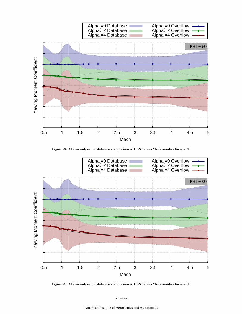
Figures 23 through 25 are plots of the yawing-moment coefficient (CLN) versus Mach for φ = 45, 60, and90 degrees. The agreement between the CFD data and the nominal database values is excellent. Althoughnot shown here, the agreement between the CFD CLN and the database CLN is excellent for all φ angles.

Figure 26 is a plot of the rolling-moment coefficient (CLL) versus Mach number for φ = 45 degrees.It can be seen that the unsteady oscillations in the CFD data are relatively large compared to the databaseuncertainty. While the CFD values fall within the database uncertainty, the agreement at αt = 4.0 degrees isnot very good.

The differences between the CFD data and the nominal aerodynamic data can be due to a number offactors. These factors include limitations in the accuracy of the CFD, including inherent assumptions inunsteady RANS modeling and the ability of the turbulence model to reproduce the flow physics. These alsoinclude the large differences in Reynolds number between the wind-tunnel test and the flight vehicle, thepossibility of strong wind-tunnel wall effects in the transonic and low supersonic ranges, and sting effects.The geometry of the wind-tunnel model is of realtively low fidelity due to the 0.8% scale of the model, and

14 of 35


Nor

mal

For

ce C

oeffi

cien

t

Mach

PHI = 30



0.5 1 1.5 2 2.5 3 3.5 4 4.5 5


Nor

mal

For

ce C

oeffi

cien

t

Mach

PHI = 60



0.5 1 1.5 2 2.5 3 3.5 4 4.5 5


15 of 35


Nor

mal

For

ce C

oeffi

cien

t

Mach

PHI = 300



0.5 1 1.5 2 2.5 3 3.5 4 4.5 5


Nor

mal

For

ce C

oeffi

cien

t

Mach

PHI = 315



0.5 1 1.5 2 2.5 3 3.5 4 4.5 5


16 of 35


Nor

mal

For

ce C

oeffi

cien

t

Mach

PHI = 330



0.5 1 1.5 2 2.5 3 3.5 4 4.5 5


Sid

e F

orce

Coe

ffici

ent

Mach

PHI = 45



0.5 1 1.5 2 2.5 3 3.5 4 4.5 5

Figure 17. SLS aerodynamic database comparison of CY versus Mach number for φ = 45

17 of 35


Sid

e F

orce

Coe

ffici

ent

Mach

PHI = 60



0.5 1 1.5 2 2.5 3 3.5 4 4.5 5


Sid

e F

orce

Coe

ffici

ent

Mach

PHI = 90



0.5 1 1.5 2 2.5 3 3.5 4 4.5 5


18 of 35


Pitc

hing

Mom

ent C

oeffi

cien

t

Mach

PHI = 0



0.5 1 1.5 2 2.5 3 3.5 4 4.5 5

Figure 20. SLS aerodynamic database comparison of CLM versus Mach number for φ = 0

Pitc

hing

Mom

ent C

oeffi

cien

t

Mach

PHI = 45



0.5 1 1.5 2 2.5 3 3.5 4 4.5 5


19 of 35


Pitc

hing

Mom

ent C

oeffi

cien

t

Mach

PHI = 180



0.5 1 1.5 2 2.5 3 3.5 4 4.5 5


Yaw

ing

Mom

ent C

oeffi

cien

t

Mach

PHI = 45



0.5 1 1.5 2 2.5 3 3.5 4 4.5 5

Figure 23. SLS aerodynamic database comparison of CLN versus Mach number for φ = 45

20 of 35


Yaw

ing

Mom

ent C

oeffi

cien

t

Mach

PHI = 60



0.5 1 1.5 2 2.5 3 3.5 4 4.5 5


Yaw

ing

Mom

ent C

oeffi

cien

t

Mach

PHI = 90



0.5 1 1.5 2 2.5 3 3.5 4 4.5 5


21 of 35


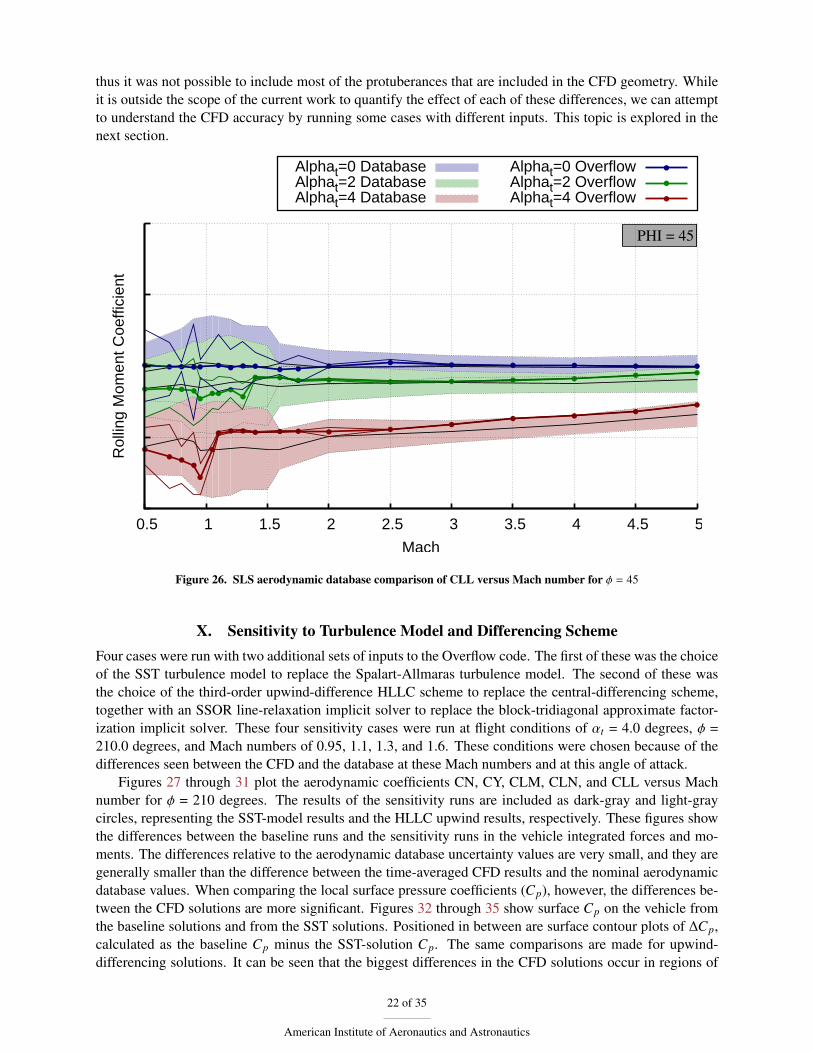
thus it was not possible to include most of the protuberances that are included in the CFD geometry. Whileit is outside the scope of the current work to quantify the effect of each of these differences, we can attemptto understand the CFD accuracy by running some cases with different inputs. This topic is explored in thenext section.

Rol

ling

Mom

ent C

oeffi

cien

t

Mach

PHI = 45



0.5 1 1.5 2 2.5 3 3.5 4 4.5 5

Figure 26. SLS aerodynamic database comparison of CLL versus Mach number for φ = 45

X. Sensitivity to Turbulence Model and Differencing SchemeFour cases were run with two additional sets of inputs to the Overflow code. The first of these was the choiceof the SST turbulence model to replace the Spalart-Allmaras turbulence model. The second of these wasthe choice of the third-order upwind-difference HLLC scheme to replace the central-differencing scheme,together with an SSOR line-relaxation implicit solver to replace the block-tridiagonal approximate factor-ization implicit solver. These four sensitivity cases were run at flight conditions of αt = 4.0 degrees, φ =210.0 degrees, and Mach numbers of 0.95, 1.1, 1.3, and 1.6. These conditions were chosen because of thedifferences seen between the CFD and the database at these Mach numbers and at this angle of attack.

Figures 27 through 31 plot the aerodynamic coefficients CN, CY, CLM, CLN, and CLL versus Machnumber for φ = 210 degrees. The results of the sensitivity runs are included as dark-gray and light-graycircles, representing the SST-model results and the HLLC upwind results, respectively. These figures showthe differences between the baseline runs and the sensitivity runs in the vehicle integrated forces and mo-ments. The differences relative to the aerodynamic database uncertainty values are very small, and they aregenerally smaller than the difference between the time-averaged CFD results and the nominal aerodynamicdatabase values. When comparing the local surface pressure coefficients (Cp), however, the differences be-tween the CFD solutions are more significant. Figures 32 through 35 show surface Cp on the vehicle fromthe baseline solutions and from the SST solutions. Positioned in between are surface contour plots of ∆Cp,calculated as the baseline Cp minus the SST-solution Cp. The same comparisons are made for upwind-differencing solutions. It can be seen that the biggest differences in the CFD solutions occur in regions of

22 of 35


Nor

mal

For

ce C

oeffi

cien

t

Mach

PHI = 210



SST ModelHLLC Upwind

0.5 1 1.5 2 2.5 3 3.5 4 4.5 5


Sid

e F

orce

Coe

ffici

ent

Mach

PHI = 210




0.5 1 1.5 2 2.5 3 3.5 4 4.5 5


23 of 35


Pitc

hing

Mom

ent C

oeffi

cien

t

Mach

PHI = 210




0.5 1 1.5 2 2.5 3 3.5 4 4.5 5


Yaw

ing

Mom

ent C

oeffi

cien

t

Mach

PHI = 210




0.5 1 1.5 2 2.5 3 3.5 4 4.5 5


24 of 35


Rol

ling

Mom

ent C

oeffi

cien

t

Mach

PHI = 210




0.5 1 1.5 2 2.5 3 3.5 4 4.5 5

Figure 31. SLS aerodynamic database comparison of CLL versus Mach number for φ = 210

shock interactions and regions of flow separation from the surface of the vehicle.Comparisons of the sectional loads in the normal and lateral directions on the core and SRBs are shown

in Fig. 36 for M = 1.1, and in Fig. 37 for M = 1.6. The M = 1.1 differences in the loads between the cases aresubstantial, especially for the lateral loads on the core. The biggest differences seen in the SST turbulence-model solutions appear to be in regions with flow separation, for example, near the forward and aft attachhardware. The biggest differences seen in the HLLC upwind-scheme solutions appear to be in high-pressuregradient regions caused by shock waves.

XI. Booster SeparationThe SLS launch vehicle includes two solid-rocket boosters that burn out before the primary core stage andthus must be discarded during the ascent trajectory. Because gravity is not acting in a way that pulls theexpended boosters away from the core, and aerodynamic loads also do not act in a way to substantiallyencourage separation, small rockets called Booster Separation Motors (BSMs) are used to actively push theboosters away from the core. There are 16 of these BSMs—four forward BSMs and four aft BSMs on eachbooster. The forward BSMs fire in a partially forward (upstream-facing) direction, which results in complexplumes and interactions of those plumes with the high-speed freestream flow, and with the core stage ofthe vehicle. In addition, the low dynamic pressure during the separation event combined with the relativelyhigh-thrust separation motors means that the plume affects a very large volume of flow on the scale of theSLS vehicle itself. To top this all of this off, the flow is unsteady. In addition to the complex flow physics,the biggest challenge for creating a booster-separation aerodynamic database are the large number of basisvariables, including orientation of the core, relative position and orientation of the boosters, and rocket thrustlevels.

The design of the SRBs is relatively unchanged from that used with the Space Shuttle Launch Vehicle,which has a rich flight history. However, the difference between the SLS core and the Space Shuttle ExternalTank results in much narrower clearances during SRB separation. In addition, the placement of the main

25 of 35


a) Baseline and SST turbulence model b) Baseline and HLLC upwind differencing

Figure 32. Surface Cp and ∆Cp at Mach 0.95

26 of 35




27 of 35




28 of 35




29 of 35


a) Normal sectional loads on core b) Lateral sectional loads on core

c) Normal sectional loads on left booster (SRBM) d) Normal sectional loads on right booster (SRBP)

e) Lateral sectional loads on left booster (SRBM) f) Lateral sectional loads on right booster (SRBP)

Figure 36. Sectional aerodynamic loads for turbulence-model and differencing-scheme sensitivity cases on the solid rocketboosters at Mach 1.1

30 of 35


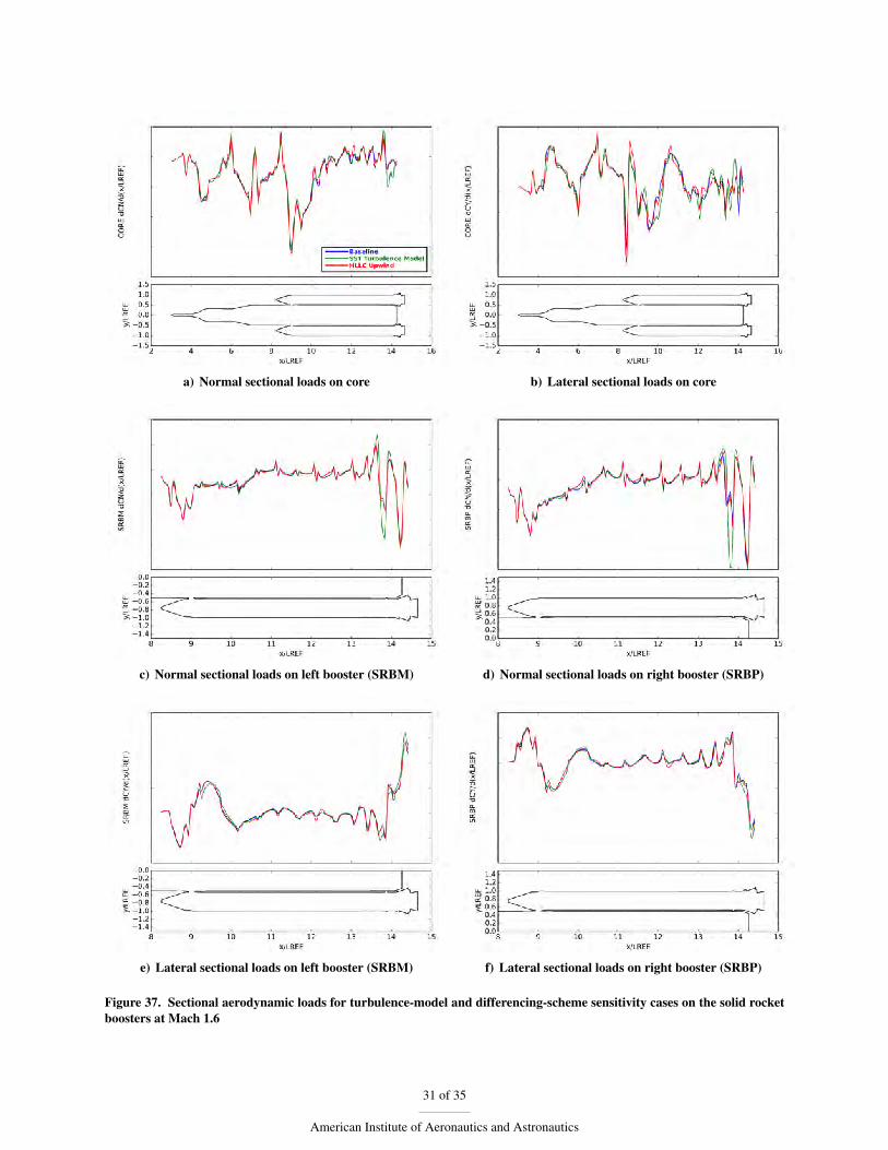
a) Normal sectional loads on core b) Lateral sectional loads on core

c) Normal sectional loads on left booster (SRBM) d) Normal sectional loads on right booster (SRBP)

e) Lateral sectional loads on left booster (SRBM) f) Lateral sectional loads on right booster (SRBP)

Figure 37. Sectional aerodynamic loads for turbulence-model and differencing-scheme sensitivity cases on the solid rocketboosters at Mach 1.6

31 of 35


engines at the base of the core results in the main-engine plumes being directly in the path of the separatingSRBs as they move away from the core, causing a plume interaction that was not present during separationfrom the Space Shuttle Launch Vehicle. Because of these additional challenges, it is necessary to reduceaerodynamic uncertainty as much as possible in order to clear the integrated system for flight.

Because of the very large run matrix required to create a database for the range of possible configurationsthat occur during separation, an inviscid flow solver with output-based adaptive meshing called Cart3D[19, 20] was selected as the primary analysis tool. This tool requires only a surface grid and flow solverinputs to run; volume mesh creation is automatic. Combined with the adaptive mesh capability, this meansthat quality solutions can be obtained with only minimal oversight by the user. Figure 38 shows an exampleof the mesh adaptation results for a case soon after separation, in which the BSMs are firing, and the SRBsare close to the core. The initial mesh, in Fig. 38a, has 416 thousand volume cells, and the final mesh has 13million. A mesh growth ratio of 1.5 was used for the first two adaptation cycles, and the remaining cyclesused a growth ratio of 2.0. This calculation took 1.5 hrs using 20 CPUs on a single Ivy Bridge node.

The forward BSMs cause a strong shock to form as far upstream as the MPCV service module, and theflow is subsonic behind this shock. The mesh adaptation history demonstrates how relatively high resolutionis required quite far off of the body. Thus a single grid able to resolve all flow conditions in the databasewould have an excessively high number of cells.

To support the SLS project, a new booster-separation aerodynamic database is currently being produced.Comparisons will be made to viscous Overflow results, which will provide insights that are hard to predictfor a database with complex flow and many degrees of freedom. The procedures for this work will follow thelessons learned to perform first-stage separation analysis that supported Ares I [4, 21]. In addition, a windtunnel study performed at NASA Langley Research Center’s Unitary Plan Wind Tunnel in September andOctober of 2014 will be used to provide validation for the computational aerodynamic database. Because ofthe range of geometric scales, from booster separation motors with throat planes several inches in diameterto the overall vehicle length of more than 300 ft, completing a wind tunnel test to support the aerodynamicdatabase was judged to be prohibitively expensive. As a result, the CFD database generated in this work isa high-priority analysis for the mission success of SLS.

ConclusionsThe current CFD effort has delivered valuable data products to the SLS program in support of the de-velopment of the new space-launch capability. Over 28 million CPU hours were used to run Overflowsimulations for 739 flight conditions covering a wide range of ascent Mach numbers, total angles of attack,and roll angles. CFD derived data has been delivered to the program in the form of sectional line loads,surface Cp, vent-location pressures and boundary-layer data, and aerodynamic loads on all of the vehicle’sprotuberances. Favorable comparisons were found between the CFD flight-vehicle aerodynamics and thewind-tunnel derived aerodynamic database. The regions of largest discrepancy occur in the transonic Machrange, a flight regime with complex shock interactions and unsteady flows, and a range which presents sig-nificant challenges to the wind-tunnel testing. Four of the cases were run to evaluate the solutions using adifferent turbulence model, and also with an upwind differencing scheme. The differences in the integratedforces and moments are relatively small, but there are larger local differences in Cp in regions with shockwaves and separated flow.

Analysis of the aerodynamics during booster separation using the Cart3D unstructured Cartesian solveris also being performed for the program. These simulations benefit greatly from the use of output-basedadaptive meshing. The complex flow physics generated by 16 booster-separation motors firing into thesupersonic flow-field requires resolution of many off-body flow features. This analysis work will continuein the near future as the program builds an aerodynamic database which will be used to ensure successfulbooster separation. The large number of basis variables will require tens of thousands of simulations. Theaccuracy of the simulations will be assessed by comparison to newly acquired wind-tunnel data, with thegoal of reducing the aerodynamic uncertainty within the database.

32 of 35


a) Initial mesh, 0 adaptation cycles b) After 2 adaptation cycles

c) After 3 adaptation cycles d) After 4 adaptation cycles

e) After 5 adaptation cycles f) After 6 adaptation cycles

Figure 38. Grid history of static pressure on vehicle surface and center xz-plane cut for case with BSMs firing

33 of 35


AcknowledgmentsThis current work was made possible by the the hard work of many individuals. The authors wish toacknowledge the following individuals for their contributions to defining the initial geometry, to the gridgeneration, and to the flow-solver inputs. Thanks go to Jeffrey Housman, William Chan, Emre Sozer, ShayanMoini-Yekta, H. Dogus Akaydin, Jeff Onufer, Goetz Klopfer, and Cetin Kiris. We wish to acknowledge theexpertise and hard work of the people of the NASA Advanced Supercomputing Division. Their world-classfacility made it relatively easy to utilize millions and millions of CPU hours.

References[1] Gomez, R. J., Vicker, D., Rogers, S. E., Aftosmis, M. J., Chan, W. M., Meakin, R. L., and Murman, S., “STS-107

Investigation Ascent CFD Support,” 34th AIAA Fluid Dynamics Conference, June 2004, AIAA Paper 2004-2226.

[2] Murman, S. M., Aftosmis, M. J., and Rogers, S. E., “Characterization of Space Shuttle Ascent Debris UsingCFD Methods,” 43rd AIAA Aerospace Sciences Meeting and Exhibit, June 2005, AIAA Paper 2005-1223.

[3] Tejnil, E. and Rogers, S. E., “CFD Assessment of Forward Booster Separation Motor Ignition Overpressure onET XT 718 Ice/Frost Ramp,” 50th AIAA Aerospace Sciences Meeting, January 2012, AIAA Paper 2012-0673.

[4] Pamadi, B. N., Pei, J., Pinier, J. T., Holland, S. D., and Covell, P. F., “Aerodynamic Analyses and DatabaseDevelopment for Ares I Vehicle First-Stage Separation,” Journal of Aircraft, Vol. 49, No. 5, 2012, pp. 864–874.

[5] Kiris, C., Housman, J., Gusman, M., Schauerhamer, D., Deere, K., Elmiligui, A., Abdol-Hamid, K., Parlette,E., Andrews, M., and Blevins, J., “Best Practices for Aero-Database CFD Simulations of Ares V Ascent,” 49thAIAA Aerospace Sciences Meeting, January 2011, AIAA Paper 2011-16.

[6] Gusman, M., Housman, J., and Kiris, C., “Best Practices for CFD Simulations Launch Vehicle Ascent withPlumes - OVERFLOW Perspective,” 49th AIAA Aerospace Sciences Meeting, January 2011, AIAA Paper 2011-1054.

[7] Aftosmis, M. A. and Rogers, S. E., “Effects of Jet-Interaction on Pitch-Control of a Launch Abort Vehicle,” 46thAIAA Aerospace Sciences Meeting and Exhibit, January 2008, AIAA Paper No. 2008-1281.

[8] Childs, R. E., Garcia, J. A. Melton, J. A., Rogers, S. E., Shestopovlov, A. J., and Vicker, D. J., “OverflowSimulation Guidelines for Orion Launch Abort Vehicle Aerodynamic Analyses,” June 2011, AIAA Paper 2011-3163.

[9] Rogers, S. E. and Pulliam, T. H., “Computational Challenges in Simulating Powered Flight of the Orion LaunchAbort Vehicle,” 29th AIAA Applied Aerodynamics Conference, June 2011, AIAA Paper 2011-3339.

[10] Childs, R. E., Garcia, J. A., Rogers, S. E., and Vicker, D. J., “Overflow Aerodynamic Simulation of the OrionLaunch Abort Vehicle,” JANNAF 33rd Exhaust Plume and Signatures Meeting, December 2012.

[11] Vicker, D. J., Childs, R. E., Rogers, S. E., McMullen, M. S., Garcia, J. A., and Greathouse, J. S., “Effects ofthe Orion Launch Abort Vehicle Plumes on Aerodynamics and Controllability,” 51st AIAA Aerospace SciencesMeeting, January 2013, AIAA Paper 2013-0970.

[12] Nichols, R. H., Tramel, R. W., and Buning, P. G., “Solver and Turbulence Model Upgrades to OVERFLOW2for Unsteady and High-Speed Applications,” 36th AIAA Fluid Dynamics Conference, June 2006, AIAA Paper2006-2824.

[13] Chan, W. M., “Developments in Strategies and Software Tools for Overset Structured Grid Generation andConnectivity,” 20th AIAA Computational Fluid Dynamics Conference, June 2011, AIAA Paper 2011-3051.

[14] Rogers, S. E., Roth, K., Nash, S. M., Baker, M. D., P., S. J., Whitlock, M., and Cao, H. V., “Advances in OversetCFD Processes Applied to Subsonic High-Lift Aircraft,” 18th AIAA Applied Aerodynamics Conference, June2000, AIAA Paper 2000-4216.

[15] Spalart, P. R. and Allmaras, S. R., “A One-Equation Turbulence Model for Aerodynamic Flows,” RechercheAerospatiale, Vol. 1, 1994, pp. 5.

[16] Menter, F. R., “Two-Equation Eddy-Viscosity Turbulence Models for Engineering Applications,” AIAA Journal,Vol. 32, No. 8, 1994, pp. 1598.

34 of 35


[17] Menter, F. R., Kuntz, M., and Langtry, R., “Ten Years of Industrial Experience with the SST Turbulence Model,”Turbulence, Heat and Mass Transfer, Vol. 4, 2003, pp. 625.

[18] Pandya, S. and Chan, W. M., “Computation of Sectional Loads from Surface Triangulation and Flow Data,” 20thAIAA Computational Fluid Dynamics Conference, June 2011, AIAA Paper 2011-3680.

[19] Aftosmis, M., Berger, M., and Adomavicius, G., “A Parallel Multilevel Method for Adaptively Refined CartesianGrids with Embedded Boundaries,” 38th Aerospace Sciences Meeting, January 2000, AIAA Paper 2000-0808.

[20] Nemec, M. and Aftosmis, M., “Adjoint Error Estimation and Adaptive Refinement for Embedded-BoundaryCartesian Meshes,” 18th AIAA Computational Fluid Dynamics Conference, June 2007, AIAA Paper 2007-4187.

[21] Klopfer, G. H., Onufer, J. T., Pandya, S. A., Chan, W. M., Kless, J. E., and Lee, H. C., “Analyses of the Ares IA106-Plus Launch Vehicle First Stage Separation,” Tech. Rep. FS-TR-00002, NASA, 2011.

35 of 35


Documents

CFD Simulations of the Space Launch System Ascent