Embed Size (px)
Citation preview

SPACAR User Manual
dr. ir. R. G. K. M. Aarts, dr. ir. J. P. Meijaard and prof. dr. ir. J. B. Jonker
2011 Edition, March 21, 2011
Report No. WA-1299


Table of contents
Preface iii
1 The SPACAR program 11.1 Introduction . . . . . . . . . . . . . . . . . . . . . . . . . . . . . . . . . . . . 11.2 SPACAR and MATLAB . . . . . . . . . . . . . . . . . . . . . . . . . . . . . 11.3 SPAVISUAL . . . . . . . . . . . . . . . . . . . . . . . . . . . . . . . . . . . 101.4 SPASIM and SIMULINK . . . . . . . . . . . . . . . . . . . . . . . . . . . . . 111.5 Perturbation method and modal techniques . . . . . . . . . . . .. . . . . . . . 13
2 Keywords 152.1 Introduction . . . . . . . . . . . . . . . . . . . . . . . . . . . . . . . . . . . .152.2 Kinematics . . . . . . . . . . . . . . . . . . . . . . . . . . . . . . . . . . . . 162.3 Dynamics . . . . . . . . . . . . . . . . . . . . . . . . . . . . . . . . . . . . . 252.4 Inverse dynamics (setpoint generation) . . . . . . . . . . . . .. . . . . . . . . 34
2.4.1 Trajectory generation . . . . . . . . . . . . . . . . . . . . . . . . . .. 342.4.2 Nominal inputs and reference outputs . . . . . . . . . . . . . .. . . . 39
2.5 Linearization . . . . . . . . . . . . . . . . . . . . . . . . . . . . . . . . . . .412.6 Non-linear simulation of manipulator control . . . . . . . .. . . . . . . . . . 45
3 Examples 473.1 Planar sliding bar . . . . . . . . . . . . . . . . . . . . . . . . . . . . . . . .. 473.2 Planar slider–crank mechanism . . . . . . . . . . . . . . . . . . . . .. . . . . 493.3 Cardan-joint mechanism . . . . . . . . . . . . . . . . . . . . . . . . . . . .. 573.4 Planar four-bar mechanism . . . . . . . . . . . . . . . . . . . . . . . . .. . . 603.5 Rotating mass–spring system . . . . . . . . . . . . . . . . . . . . . . . .. . . 633.6 Cantilever beam in Euler buckling . . . . . . . . . . . . . . . . . . . .. . . . 663.7 Cantilever beam subject to concentrated end force . . . . . .. . . . . . . . . . 683.8 Short beam . . . . . . . . . . . . . . . . . . . . . . . . . . . . . . . . . . . . 713.9 Lateral buckling of cantilever beam . . . . . . . . . . . . . . . . .. . . . . . 733.10 State-variable and output equations . . . . . . . . . . . . . . .. . . . . . . . . 763.11 Rigid spatial manipulator mechanism . . . . . . . . . . . . . . . .. . . . . . 79
i

ii Table of contents
3.12 Flexible spatial manipulator mechanism . . . . . . . . . . . .. . . . . . . . . 893.13 Chord-driven underactuated robotic finger . . . . . . . . . . .. . . . . . . . . 903.14 Tricycle . . . . . . . . . . . . . . . . . . . . . . . . . . . . . . . . . . . . . . 933.15 Screw motion . . . . . . . . . . . . . . . . . . . . . . . . . . . . . . . . . . . 98
A SPACAR installation 101
B SPACAR error messages 103
C MATLAB tutorial 105C.1 Basic MATLAB graphics commands . . . . . . . . . . . . . . . . . . . . . . .105C.2 Quitting and saving the workspace . . . . . . . . . . . . . . . . . . . .. . . . 107
References 109
Preface
This is the 2011 edition of the manual that describes the use of the SPACAR-package in aMAT-LAB /SIMULINK environment. This software is being developed at the Laboratory of Mechani-cal Automation of the Faculty of Engineering Technology, University of Twente, and is partlybased on work carried out at the Laboratory for Engineering Mechanics, Delft University ofTechnology.This manual accompanies the 2011 UT-release ofSPACAR. With respect to the previous edi-tions of this manual new keywords have been included reflecting changes in the software. Inparticular, the screw and tube elements are included. TheSPAVISUAL manual is separated fromthis manual and reflects the extensive revision of this visualization program. Some exampleshave been added to show the use of the new elements.The references to sections and examples in the lecture notes[1] are updated for the 2005 editionof these lecture notes. They may be only approximate for other editions.The visualisation toolSPAVISUAL has been implemented by Jan Bennik and later extended byTjeerd van der Poel and Steven Boer, who also provided the separate manual for this tool.Corrections of errors, suggestions for improvements and other comments are welcome.
March 21, 2011, dr. ir. R. G. K. M. Aarts (Email:[email protected] ), dr. ir.J. P. Meijaard and prof. dr. ir. J. B. Jonker.
iii

iv Preface

1
The SPACAR program
1.1 Introduction
The computer programSPACARis based on the non-linear finite element theory for multi-degreeof freedom mechanisms as described in Jonker’s lecture notes on the Dynamics of Machinesand Mechanisms [1]. The program is capable of analysing the dynamics of planar and spatialmechanisms and manipulators with flexible links and treats the general case of coupled largedisplacement motion and small elastic deformation. The motion can be simulated by solving thecomplete set of non-linear equations of motion or by using the so-called perturbation method.The computational efficiency of the latter method can be improved further by applying modaltechniques.In this chapter, an outline of theSPACARpackage for use withMATLAB andSIMULINK is givenin the next sections. For instance, for the design of mechanical systems involving automaticcontrols (such as robotic manipulators), interfaces withMATLAB [2] are provided for open-loop system analyses, Section 1.2. Open-loop and closed-loop simulations can be carried outwith blocks from aSIMULINK library, Section 1.4. A special visualization tool,SPAVISUAL, isdescribed in Section 1.3. Additional tools are available for using the perturbation method andthe modal techniques inSIMULINK (Section 1.5). Installation notes forSPACAR are given inAppendix A.A graphical user interface (GUI) for generating input files for spatial systems is available andwill be further developed. People interested in rigid planar mechanisms may consider the useof the commercially available packageSAM by ARTAS [4]. It has a nice graphical interface forthe definition of mechanisms and it provides more elements thanSPACAR.
1.2 SPACAR and MATLAB
TheSPACARprogram system for use in theMATLAB environment contains five modules, whichobtain their input from format-free user-supplied data. Inthe following a short description ofevery module will be given. The functional connections between the modules are illustrated inFig. 1.1.
1

2 Chapter 1. The SPACAR program
KIN
INVDYN
DYN
STATIO
LINEAR
mode 1
mechanism
connectivity
configuration
DOFs q =
(xm, em)
dynamic
properties
forces
(fm, σm)
trajectory path
velocity profile
(xp
o, xp
o)
DOFs ( q, q)
joint variables (em
0, em, σm
0)
nominal inputs (u0)
reference outputs (y0)
mode 2
State space matricesmode 3
mode 4
mode 7
mode 8
mode 9
Linearized equation
Eigen frequencies
Buckling loads
State space matrices
LINEAR
Figure 1.1. Functional relations between modules inSPACAR. The indicated modes areavailable in theMATLAB environment.
KIN is the kinematics module that analyses the configuration of the mechanism. The kinematicproperties of the motion are specified by the geometric transfer functions. The followingsteps are provided by theKIN -module:
1. Definition of the mechanism connectivity, the configuration and the degrees of free-dom (DOFs),q = (x(m),e(m)).
2. System preparation.
3. Calculation of the geometric transfer functions.
DYN is the dynamics module that generates the equations of motion and performs numericalintegration in the forward dynamic analysis (in the so-calledmode=1 of SPACAR). Fur-thermore, it generates and solves the equations for the kinetostatic analysis.
INVDYN is the inverse manipulator dynamics module that performs the inverse kinematics anddynamics (mode=2) and generates the setpoints for the simulation of manipulator motionwith closed-loop control inSIMULINK (see Sect. 1.4). The system inputs, represented bythe nominal input vectoru0, are to be varied by the control system actuators. The systemoutputs, represented by the reference output vectory0, consist of the coordinates to bemonitored by control sensors. Coordinates that are not measured may be added to checkthe performance of the manipulator in the simulation.
STATIO computes stationary solutions of autonomous systems. Stationary solutions are solu-tions in which the vector of dynamic degrees of freedomqd has a constant value. Thiscan represent a static equilibrium configuration or a state of steady motion.
LINEAR is a forward dynamics stage for the generation of linearizedequations and state spacematrices. It can be used in different modes as described below.

Section 1.2. SPACAR and MATLAB 3
In mode=4 the LINEAR module is an extension of the forward dynamic analysis (mode=1)where coefficient matrices of the linearized equations are calculated as functions of the set ofdegrees of freedomq. If there are only holonomic deformations in a system, the linearizedequations are generated in the form:
M 0δq + [C0 + D0] δq + [K0 + N 0 + G0] δq = DF(x)T0 δf − DF
(e)T0 δσa, (1.1)
whereM 0 is the reduced mass matrix,C0 the velocity sensitivity matrix,D0 the damping ma-trix, K0 the structural stiffness matrix, andN 0 andG0 are the dynamic and geometric stiffnessmatrices respectively. External and internal driving forces are represented by the vectorsδfandδσa, respectively. In addition, if input and output vectorsδu andδy are defined also thelinearized state equations and output equations are computed (seemode=9).In mode=3 locally linearized models are generated about a predefined nominal trajectory wherethe output data (setpoints) from the inverse dynamics module (i.e. a previousmode=2 run) areused. In addition to the coefficient matrices, a complete state space system is generated andwritten to a so-calledltv file (see Sect. 1.5). In the case of a flexible mechanism additionaldegrees of freedom describing the elastic behaviour of the mechanism have to be included inthe dynamic models (bothmode=2 and3). At this stage in the so-called “rigidified” model,these flexibilities are prescribed zero, i.e.εm
i ≡ 0.In mode=7 eigenvalues (frequencies) and corresponding eigenvectors of the state space ma-trix A are computed for a static equilibrium configuration or a state of steady motion. Theassociated frequency equation of the undamped system is given by
det(
−ω2i M
dd
0 + Kdd0 + N dd
0 + Gdd0
)
= 0, (1.2)
where the quantitiesωi are the natural frequencies of the system.In mode=8 a linear buckling analysis is carried out for a static equilibrium configuration or astate of steady motion. Critical load parametersλi are determined by solving the eigenvalueproblem:
det(Kdd0 + λiG
dd0 ) = 0, (1.3)
where the load multipliers satisfy
f i = λif 0. (1.4)
Here,Kdd0 is the structural stiffness matrix andGdd
0 is the geometric stiffness matrix due to thereference loadf 0 giving rise to the reference stressesσ0. f i represents the bucking load thatcorresponds withλi. In addition, directional nodal compliances are computed.In mode=9 linearized equations for control system analysis are computed for a static equilib-rium configuration or a state of steady motion and are generated in the form:
Mdd
0 δqd +[
Cdd0 + Ddd
0
]
δqd +[
Kdd0 + N dd
0 + Gdd0
]
δqd = B0δu, (1.5)
where
B0 =[
DqdF(x)T0 | − DqdF
(e)T0 | − M
dr
0 | −(
Cdr0 + Ddr
0
)
| −(
Kdr0 + N dr
0 + Gdr0
)]
(1.6)
is the input matrix and
δu =[
δf (c,m)T , δσ(m,c)Ta , δqrT , δqrT , δqrT
]T(1.7)

4 Chapter 1. The SPACAR program
is the input vector. The vectorsδqrT , δqrT , δqrT represent the prescribed (input) accelerations,velocities and displacements respectively. The linearized equations can be transformed into thelinearized state space form:
δz = Aδz + Bδu,
δy = Cδz + Dδu,(1.8)
whereA is the state matrix,B the input matrix,C the output matrix andD the feed throughmatrix. The state vectorδz is defined byδz = [δqdT , δqdT ]T , whereδqd is the vector ofdynamic degrees of freedom. The matricesB, C andD depend on the chosen input vectorδuand the output vectorδy. Details of the linearization are discussed in Chapter 12 of the lecturenotes.
Systems with non-holonomic deformations
For systems with non-holonomic deformations arising from wheel elements, the above descrip-tion has to be modified in several respects. Onlymode=0, mode=1, mode=4, mode=7 andmode=9 are supported. The state vector consists of the coordinatesdescribing the configura-tion,qk, and the velocity coordinates,qd. The configuration coordinates are split in coordinateswhose derivatives are velocity coordinates and coordinates that have no corresponding velocitycoordinates; the latter are called kinematic coordinates.The dynamic equations consist of twoparts, the kinematic differential equations defining the derivatives of the configuration coordi-nates and the equations of motion defining the time derivatives of the velocity coordinates.The linearized equations have the form
[
I O
O M 0
] [
δqk
δqd
]
+
[
−Bk0 −Ak0
K0 + N 0 + G0 C0 + D0
] [
δqk
δqd
]
=
[
0
DF(x)T0 δf − DF
(e)T0 δσa
]
, (1.9)
whereAk0 andBk0 are kinematic matrices. For ordinary systems,Bk0 is a zero matrix andAk0 is an identity matrix. Formode=7, a stationary solution is first obtained with the moduleSTATIO and the eigenvalues are obtained by solving the characteristic equation
det
[
Iλ − Bk0 −Ak0
K0 + N 0 + G0 M 0λ + C0 + D0
]
= 0. (1.10)
Formode=9, the linearized state equations are obtained as in equation(1.8), with the differencethat the variations in the states are nowδz = [δqkT , δqdT ]T .
Definition of a mechanism model
A model of a mechanism must be defined in an input file of file type(or file name extension)dat . This input file consists of a number of keywords with essential and optional parameters.The input file can be generated with any text editor.In Chapter 2 the meaning of the keywords and their parameters is discussed in detail. In theexamples in Chapter 3 complete input files are presented.

Section 1.2. SPACAR and MATLAB 5
Running SPACAR in the MATLAB environment
Once the mechanism is defined and this information is saved toa dat input file, SPACAR canbe activated with theMATLAB command
>> spacar(mode,’filename’)
Here,mode indicates the type of computation as shown in Fig. 1.1.filename is the nameof the input file, without the extension.dat . Thefilename is limited to 20 characters fromthe set “0”–“9”, “a”–“z”, “A”–“Z” and “ ”, so it can not include drive or path specifications.The linearization withmode=3 needs data from a previous inverse dynamics computation. Tothat end the specifiedfilename is truncated with at least one character at the right until avalid output data file is found. So e.g.spacar(3,’testlin’) can use data from an earlierspacar(2,’test’) computation. If no data file can be found in this way the linearizationis aborted.During the computation a plot of the mechanism is shown in a separate window. While thesimulation is running anAbort button is activated in the plot area. Pressing this button willterminate the simulation (possibly after some delay). To speed up the computation, the plot canbe disabled by specifying the mode with a minus sign, e.g.mode=-2 for an inverse dynamicscomputation without a continually updated plot. The plotting utility spadraw can also be usedafter the simulation to visualize the results, see page 10.During the computations the results are stored in one or moredata files and inMATLAB arrays.A log file is always created whenSPACARstarts processing the inputdat file. This log filecontains an analysis of the input and possible errors and warnings. It is described in more detailon page 8. Some errors in the input file do not lead to an early termination of theSPACAR
computation, but nevertheless give unusable results. Therefore it is advisable to check thelogfile for unexpected messages.All other data files are so-calledSPACAR binary data files (SBF), which implies that these arein a binary format and cannot be easily read by a user. Therefore, utilities are provided to readand modify data in these files, see page 9. Depending on themode up to three binary outputfiles may be created.For all modes aSPACARbinary data file with filename identical to the input file and extensionsbd is written. The contents of this file are also stored inMATLAB arrays, that are of courseimmediately available in theMATLAB workspace e.g. to be visualized with the standardMAT-LAB graphics commands, such asplot (see e.g. Chapter 3 and Appendix C). The followingvariables are created or overwritten:
mode SPACARmode numberndof number of DOFs including rheonomic onesnddof number of dynamic DOFsnkdof number of configuration coordinates including rheonomic onesnkddof number of configuration coordinatesnx number of coordinatesne number of deformation parametersnxp number of fixed, calculable, input, dynamic and
kinematic coordinatesnep number of fixed, calculable, input, dynamic and
kinematic deformation parameterslnp location matrix for the nodes *1

6 Chapter 1. The SPACAR program
le location matrix for the elements *1ln connection matrix for the nodes in the elements *2it list of element types *2kdform information about quadratic terms in strains for elements *2rxyz initial orientations of elements *2rxyzq initial orientations of elements at second node *2dr0 geometric data of elements *2estiff stiffness parameters of elementsedamp damping parameters of elementsem mass per unit of length of elementseinit initial deformations of elementsesig initial stresses of elementsrl0 undeformed length of elementstime time column vectorx coordinates (nodal displacements)xd nodal velocitiesxdd nodal accelerationsfx prescribed nodal forces/momentsfxgrav gravity nodal forces/momentsfxtot reaction forces/momentse generalized deformationsed velocities of generalized deformationsedd accelerations of generalized deformationssig generalized stress resultantsdec first order geometric transfer function for the deformations DF
c(e) *3dxc first order geometric transfer function for the coordinatesDF
c(x) *3de first order geometric transfer function for the deformations DF
(e) *3dx first order geometric transfer function for the coordinatesDF
(x) *3d2e second order geometric transfer function for the deformationsD2
F(e) *3
d2x second order geometric transfer function for the coordinatesD2F
(x) *3xcompl location vector for directional nodal compliances *4
Notes:
∗1 The two location matrices provide information to find the location of a specific quantity inthe data matrices:
lnp location matrix for the nodes. The matrix elementlnp(i,j) denotesthe location of thej th coordinate (j =1..4) of nodei .
le location matrix for the elements. The matrix elementle(i,j) denotesthe location of thej th generalized deformation (j =1..6) of elementi .
The locations of undefined or unused coordinates and deformations equal zero.
For example, thex- andy-coordinates of node 7 can be shown as function of time in agraph by typing
>> plot(time,x(:,lnp(7,1:2)))

Section 1.2. SPACAR and MATLAB 7
and the first generalized stresses in elements 1, 2 and 3 can beplotted by typing
>> plot(time,sig(:,le(1:3,1)))
Obviously, storage in thex , xd , xdd , fx , e, ed , edd andsig matrices is likex(t,k)wheret is the time step andk ranges from 1 tonx for x , xd , xdd andfx , fxtot andfrom 1 tone for e, ed , edd andsig , respectively.
∗2 The variablesln , it , rxyz andrxyzq are mainly intended for internal use in the drawingtool spadraw . More user-friendly information is available in thelog file, page 8.
∗3 The (large) variablesdec , dxc , de , dx , d2e andd2x are only created if the parametersof theLEVELLOGare set accordingly, Sect. 2.2.
∗4 After a linearization run (mode=8) directional nodal compliances (inverse stiffnesses) arecomputed. Using the location matrix,xcompl(lnp(i,j)) gives this quantity for thej th coordinate (j =1..4) of nodei .
After a linearization run (mode=3, 4, 7, 8 or 9) the coefficient matrices are stored in aSPACAR
binary matrix file with extensionsbm. Besidesnnom (see infra) andtime , the accompanyingMATLAB matrices are:
m0 reduced mass matrixM 0 *5b0 input matrixB0 *5, *6c0 velocity sensitivity matrixC0 *5d0 damping matrixD0 *5k0 structural stiffness matrixK0 *5n0 geometric stiffness matrixN 0 *5g0 geometric stiffness matrixG0 *5ak0 kinematic matrixAk0 *5bk0 kinematic matrixBk0 *5
Notes:
∗5 Storage of the time-varying matrices is in a row for each timestep, so inm0(t,k) indextis the time step andk ranges from 1 tondof ×ndof . To restore the matrix structure atsome time step type e.g.reshape(m0(t,:),ndof,ndof)’ .
∗6 Only available formode=4 andmode=9.
In mode=2, 3, 4 and9 a so-calledltv file is created. The contents of this file varies and isnot automatically imported to theMATLAB workspace. From amode=2 run the following dataare available (the names identitify the data used in the file;data marked with “*” are availableat each time step):
NNOM number of (actuator) inputsNY number of outputsT time *U0 nominal input for the desired motion *Y0 reference output of the desired motion *

8 Chapter 1. The SPACAR program
In the addition the linearization runs yield additional setpoints, state space matrices and otherdata in theltv file (not all data are always present):
NNOM number of (actuator) inputsNX number of states (2×ndof )NU number of inputs (length ofU0)NY number of outputs (length ofY0)NRBM number of rigid body DOFsNYS number of outputs with 2nd order expressionNYSI index array for outputs with 2nd order expressionDFT direct feedthrough flag (D6=0)X0 initial state vectorT time *A state space system matrix *B state space input matrix *C state space output matrix *D state space direct feedthrough matrix *G second order output tensor *M0 mass matrixM 0 *C0B combined damping matrixC0 + D0 *K0B combined stiffness matrixK0 + N 0 + G0 *SIG0 generalized stress resultants *
The getss tool can be used to read the state space matrices from theltv file, see page 9.Other utilities are available to use parts of these data in aSIMULINK environment, e.g. to readsetpoints or to simulate a linear time-varying (LTV ) system (see Sect. 1.4).
The log file
Thelog file contains an analysis of the input and possible errors andwarnings that are encoun-tered. The error and warning messages are explained in more detail in Appendix B. The otheroutput can be separated into a number of blocks.The first lines indicate the version and release date of the software and a copyright note.Next the lines from the input file read by theKIN module are shown (not showing commentspresent in the input file), see also Sect. 2.2. From the analysis is written:
• The elements used in this model. The deformations of all elements are shown with theinternal numbers according to thele array and the classification of each deformation:O= fixed,C= calculable andM= DOF.
• The nodal point information with the internal numbers of thecoordinates according to thelnp array and the classification as above.
• A list showing the degrees of freedom, in which dynamic degrees of freedom are indi-cated.
• The condition number of the part of the difference matrix that has to be inverted, whichshows how well the degrees of freedom have been chosen.
The DYN module reads the next data block and processed input lines are shown. From theanalysis we get

Section 1.2. SPACAR and MATLAB 9
• The numbersNEO, NEMM, NEMandNECindicating the numbers of deformations in eachclass as explained in the lecture notes [1].
• The numbersNXO, NXC, NXMMandNXMindicating the numbers of position coordinatesin each class as explained in the lecture notes [1].
• The stiffness, damping and mass of the elements.
• The nodal point forces, mass and gyroscopic terms.
• The total mass of the system.
The zeroth, first, second and third order transfer functionsare shown next, each for the positionparameters and deformation parameters, respectively. Theamount of output can be controlledby the keywordOUTLEVELin the input file.Next for a forward analysis (mode=1 andmode=4) the name of the integrator and accuracysettings are shown. Finally a list with all time steps and thenumber of internal iterations aregiven. For an inverse dynamics analysis the trajectories and input/output definitions (see alsoSect. 2.4) are read and analysed. In case ofmode=3 the name of the data file of the previousmode=2 is shown. In case ofmode=7 the eigenvalues (frequencies) and normalized eigenvec-tors of the state system matrix are shown. In case ofmode=8 load multipliers and normalizedbuckling modes are presented. In addition the vector of directional nodal compliances is shown.
SPACAR binary data files
Some utilities are available to show, check, load or replacethe data inSPACARbinary data files(SBF). These are files with extensionssbd , sbm andltv .
checksbf checks and shows the contents of aSPACARbinary data file. The output for eachvariable is the name (“Id”), the type (1 for integer, 2 for real, 3 for text) and the size(number of rows and columns). First the “header” variables are shown with their values.Long vectors may be truncated. BetweenTDEF and TDAT the time-varying data aregiven. The number of time steps is equal to the number of rows specified forTDEF.
getfrsbf extracts a variable from aSPACARbinary data file. The “Id” must be specified andfor time-varying data the time step as well.
repinsbf replaces the value of a variable in aSPACAR binary data file. The “Id” must bespecified and for time-varying data the time step as well.
loadsbd loads all data from aSPACARbinary data (sbd ) file into MATLAB ’s workspace.
loadsbm loads all data from aSPACARbinary matrix data (sbm) file into MATLAB ’sworkspace.
getss loads the state space matrices at one time instant from aSPACAR ltv file into a statespace system inMATLAB ’s workspace.
combsbd combines data from two or moreSPACARbinary data (sbd ) files into a single outputfile. The specified output file is overwritten without a warning.

10 Chapter 1. The SPACAR program
spadraw is the plotting utility used internally bySPACAR. It can also be used to visualizeresults after a simulation has been completed.
For all utilities additional online help is available by typing help command at theMATLAB
prompt.
Limitations
The SPACAR package has some built-in limitations on the size of the manipulators that can beanalysed. Table 1.1 shows the limits for the so-called “Student version” that can be downloadedas describes in Appendix A. In case your requirements are larger, you need to contact theauthors. The licence for the freely downloadable software is time limited.
Maximum number of coordinates/deformations 175Maximum number of DOFs 20Maximum number of elements/nodal points 50Maximum number of inputs 12Maximum number of outputs 25
Table 1.1.Built-in limitations of the “Student version” of theSPACARpackage.
1.3 SPAVISUAL
SPAVISUAL is the visualization tool forSPACAR. It can visualize deformation, vibration andbuckling modes. SPAVISUAL shows beams, trusses and hinges in 2-D as well as in 3-D. Itworks with default settings which can be adjusted by the user. The only input ofSPAVISUAL
is a filename. This file has to be a.dat file which has been analysed withSPACAR. This isnecessary becauseSPAVISUAL needs the.sbd files for the deformation modes and also the.sbm files for the vibration and the buckling modes. There are somekeywords that can adjustthe default settings. Alternatively, the settings can be specified as command line options. Thesekeywords are listed in a separate manual forSPAVISUAL.SPAVISUAL is a stand-alone function inMATLAB . To run SPAVISUAL the user has to type thecommand
>> spavisual(’filename’)
or
>> spavisual(’filename’,mode)
Herefilename refers to the.dat -file that has been executed bySPACAR, andmode is themode of theSPACARanalysis.

Section 1.4. SPASIM and SIMULINK 11
1.4 SPASIM and SIMULINK
The behaviour of a manipulator mechanism with e.g. closed-loop control can be simulatedusingSIMULINK . The closed-loop simulation is defined as the problem of computing the actualtrajectory of e.g. the manipulator tip with controlled actuation of the motion. Tracking errorswith respect to a nominal prescribed trajectory can be calculated.
Rigid or rigidified link modelprescribedtrajectory
µ
hp
xp0
Flexible link model
actualtrajectory
xp
INVDYN
LINEAR
readsetpoints
read coeff.matrices
simulation
controlparameters
u0
y0
y
−
M 0,C0,K0
MATLAB analyses SIMULINK simulation
Figure 1.2. Typical overview withMATLAB analyses and aSIMULINK simulation.
Figure 1.2 shows an overview of a typical simulation scheme.The simulation is characterizedby the inverse dynamics stage, based on a rigid link model anda forward dynamic stage. Atthe forward dynamics stage the tracking behaviour of the manipulator system is studied. Inthe case of flexible manipulators additional generalized coordinates (εm
i ) describing the elasticbehaviour of the manipulator links can be used in the dynamicsystem.The block diagram in Fig. 1.3 shows a typical closed-loop simulation in more detail. Blocks areused from theSPACAR SIMULINK library spacar_lib that is part of theSPACAR package.These blocks are front-ends to so-called S-functions inSIMULINK [3]. The following blocksare provided:
1. SPASIM: the non-linear open-loop model of the manipulator with itsactuators and sen-sors. It operates in a way comparable to the forward dynamicsmode inSPACAR as dis-cussed for theMATLAB interface in Sect. 1.2. The mechanism is defined in an input datafile of file type dat . The filename of the input file must be specified. An outputlog file is written. Note that in aSIMULINK simulation the integration is determinedby theSIMULINK environment, e.g. the kind of solver, the step size and tolerances. Thedegrees of freedom of the mechanism and their first time derivatives are the “states” ofthe SPACAR S-function. The dimensions of the input and output vectors are determinedfrom the input file and should match the requirements of the otherSIMULINK blocks theyare connected to.

12 Chapter 1. The SPACAR program
ReadUnom
ReadYref
read setpoints &coeff. matrices
u0
y0
ReadM0
controlparameters
e.g. M-function
+
−controlsystem
δu
+
+
u actuatormodel
σe,m
SPASIM
S-function
mechanismmodel
em
emsensormodel
y
Figure 1.3. Block diagram of a typical closed-loop simulation inSIMULINK . The leftblocks read setpoints and coefficient matrices stored in data files during previousSPACAR
analyses (Fig. 1.1).
2. LTV: simulation of a linear time-varying system as defined in anltv file, see Sect. 1.5.
3. Setpoint U0 : reads the nominal input from anltv file with setpoints generated e.g.with mode=2 or mode=3. The filename must be specified. The setpoints are inter-polated between the specified time steps. The interpolationmethod can be chosen from:Stepwise, Linear (default) and Spline. The block has no input and the dimension of theoutput vector equals the number of nominal inputs found in the file.
4. Setpoint Sigma0 : readsσ0 from an ltv file generated with e.g.mode=3, seeSect. 1.5.
5. Reference Y0 : reads the reference output from anltv data file with setpoints. Thefilename must be specified. Interpolation is as above. This block has no input and thedimension of the output vector equals the number of reference outputs found in the file.
6. Times M0 : reads the square reduced mass matrixM 0 from anltv file generated withe.g.mode=3. The output of the block equals the input of the block is multiplied with themass matrix. Thefilename must be specified. In the case not the full dimension ofM 0 in the ltv is used, the reduced dimension has to be specified. All elements of M 0
are interpolated linearly (default) or stepwise. The dimension of the output vector equalsthe dimension of the input vector.
In the block diagram in Fig. 1.3 the output vectory of the SPASIM block is compared withthe reference output vectory0. The difference of these vectors is the input of the control sys-tem. The state matrices can be used to develop and tune a controller of any type (e.g. lin-ear, non-linear, discrete, continuous) by means of the available software tools inMATLAB andSIMULINK . The output of the controllerδu is added to the nominal input vectoru0 to actuatethe mechanism. An example is discussed in Sect. 3.11.
When using blocks from theSPACAR SIMULINK library spacar_lib note the following:
• Using any of theLTV, Setpoint U0 , Setpoint Sigma0 , Reference Y0 andTimes M0 blocks at times beyond the last time step found in the data filemay lead tounexpected results.

Section 1.5. Perturbation method and modal techniques 13
• In the current version of the software allspasim blocks in a block diagram shouldrefer to the same inputfilename . Analogously, allLTV, Setpoint U0 , SetpointSigma0 , Reference Y0 andTimes M0 must use the sameltv file.
1.5 Perturbation method and modal techniques
For systems with a larger number of degrees of freedom the required computer time for aSPASIM simulation may be unacceptable, in particular when high eigenfrequencies play a role.Then theperturbation methodmay provide a numerically efficient solution strategy.Consider e.g. the motion of the flexible manipulator depictedin Fig. 1.2. In the case the flex-ibility is taken into account, the generalized coordinatesor degrees of freedom can be writtenas
q =
[
em
εm
]
, (1.11)
whereem represent the large relative displacements and rotations and εm are the flexible de-formation parameters. Due to the flexibility the actual trajectory motion will deviate from theprescribed motion. If the deviations are small compared with the large scale motion, then the(small) vibrational motion of the manipulator can be modelled as a first-order perturbationδqof the nominal rigid link motionq0 by writing for the degrees of freedom
q = q0 + δq. (1.12)
The perturbation method involves two steps:
1. Compute nominal rigid link motionq0 from the non-linear equations of motion with allflexible deformation parametersεm ≡ 0. This analysis will also provide the nominalinput u0 of the manipulator necessary to carry out the nominal motionand the general-ized stress resultants (Langrange multipliers)σεm
0 of the rigidified deformations, i.e. theflexible deformations that are prescribed as zero.
2. Compute the vibrational motionδq from linearized equations of motion
M 0δq + C0δq + K0δq = σ0, (1.13)
whereM 0 is the reduced mass matrix,C0 includes the velocity sensitivity and dampingmatrices and all stiffness matrices are combined intoK0. The right-hand side equals
σ0 =
[
δuσεm
0
]
, (1.14)
whereδu = u − u0 is the actual control actionu minus the nominal inputu0. The pre-viously computed generalized stress resultantsσεm
0 are now applied as internal excitationforces.
To solve the linearized equations of motion (1.13) these areexpressed as a linear time varying(LTV ) system. ASPACARmode=3 run generates time-varying state space matrices that are wellsuited for this purpose. Then a typicalSPACARanalysis and linearized simulation procedure isas follows:

14 Chapter 1. The SPACAR program
• Use e.g. an inverse dynamics run (mode=2) to define the nominal motion for the rigidifiedmanipulator. Inputs and outputs of the system may be specified.
• Next the system is linearized with amode=3 call. The system is analysed along thenominal path computed previously. The elastic deformations are defined withINPUTEcommands. Inputs and outputs must be specified.
-controller
u0+
+
u
δu
σεm0
LTV
y0+
+
y
δy
Figure 1.4. Block diagram of a typical closed-loop simulation inSIMULINK based on theperturbation method.
• Finally the linearized simulation can be run with aSIMULINK model of which a typicalexample is shown in Fig. 1.4. In comparison with the non-linear simulation of Fig. 1.3 thespasim block is replaced by anLTV block that uses the linearized equations of motion.Note that now only the differences compared to the nominal motion are computed. Onlythe differenceδu of the manipulator’s input compared to the nominal input is needed. Inaddition, the generalized stress resultantsσεm
0 are part of the input of theLTV block.
In addition to the above outlined standard implementation some further extensions are provided.It is possible to include the effect of proportional controller gain, i.e. a proportional controlmatrix Kp, into the stiffness matrixK0. Of course, in that case this part of the control actionshould no longer be included in the controller in the block scheme.This approach offers advantages when subsequently a modal analysis is applied to the lineartime varying state space system. Such an analysis discriminates quasi-static behaviour of thesystem, low-frequency vibrational modes and high-frequency vibrational modes. Mostly thelatter do not significantly affect the output of the system while they can have a detrimentaleffect on the computational efficiency, even for a linearized system. With a modal analysis it ispossible to eliminate these high-frequency modes.A more profound description of the latter two techniques is currently outside the scope of thismanual.

2
Keywords
2.1 Introduction
In this chapter the user is informed about the creation of correct input data for the softwarepackageSPACAR. The input must have a specific form. Behind a number of permitted keywordsthe user supplies a list of arguments. The arguments behind akeyword are well defined. Eachmodule ofSPACAR, exceptmode=4 of LINEAR, has its own list of available keywords. Theyform blocks that are separated by the following pair of keywords:
ENDHALT
The final closure of the input is effected by:
ENDEND
The first block contains the kinematic data. The input of the mechanism model (by means ofkeywords) is treated in the “Kinematics” section 2.2. A second block of input is reserved for thedynamics module. The keywords for this block are presented in the “Dynamics” section 2.3.The solution of inverse dynamics problems demands additional input for the trajectory descrip-tion and for the definition of the input and output vectorsu0 andy0. Trajectory keywords andsystem keywords are treated in the “Inverse dynamics” section 2.4. The keywords for the lin-earization ofmode=3, mode=4 andmode=9 are given in the “Linearization” section 2.5. Atthe end of the file custom settings forSPAVISUAL can be added. The visualization toolSPAVI-SUAL is described in a separate manual. The simulation of mechanisms usingSIMULINK iscontrolled by the keywords described in the “Simulation” section 2.6.Some general remarks:
• Keywords and arguments can be separated by one or more spaces, tabs or line breaks.
• Lines must not contain more than 160 characters.
15

16 Chapter 2. Keywords
• Any text in a line following a#, %or ; is treated as a comment.
• All input is case insensitive.
• Data read from the input file are echoed in thelog file, after the comments have beenremoved and all text is transformed into upper case (capitals).
• Angles are always specified in radians.
• For some commands, such asXF andSTARTDE, not all arguments have to be specified.Default values are zero unless otherwise specified.
2.2 Kinematics
A kinematic mechanism model can be built up with finite elements by letting them have nodalpoints in common. The nodal coordinates of the finite elements are described by position andorientation coordinates. Therefore, two types of nodes aredistinguished:position or trans-lational nodes, denoted by~p for nodep, andorientationor rotational nodesdenoted by
x
p.The nodes, nodal coordinates, and deformation parameters for the truss, beam, planar bearing,hinge, pinbody (rigid beam) planar belt (gear) element and wheel elements are summarized inTable 2.1.Usually, the convention is made that nodep of an element is assigned to the lower number ofthe element nodes, and that nodeq is assigned to the higher node number. The interconnectionsbetween the elements are accomplished by indicating commonnodes between the elements.For instance, with a pin-joint connection only the translational nodes are shared. In case of ahinge-joint connection only the rotational nodes are shared whereas translational coordinatescan either be shared or unshared. When elements are rigidly connected to each other, both thetranslational and rotational nodes are shared, see Fig. 2.1. It can be observed from Table 2.1that a truss element and a hinge element do not have common nodal types and therefore cannotbe connected to each other.
pin-joint hinge-joint rigid-joint
Figure 2.1. Joint connections between finite elements.
In the first block of the kinematics module either two-dimensional (planar) or three-dimensional(spatial) elements can be specified. In the second block the initial configuration of the mecha-nism is specified. In the third block the coordinates and generalized deformations are dividedinto four groups, depending on the boundary conditions:
1. fixed prescribed coordinates (supports)2. dependent, calculable deformations3. prescribed, time-dependent coordinates4. dynamic degrees of freedom

Section 2.2. Kinematics 17
For the keywords in the third block it is important to remark that there are no keywords to fixa deformation or to release a coordinate. These are the default settings. So a deformation isfixed unless aRLSE, INPUTE or DYNEkeyword specifies otherwise. Similarly, a coordinate iscalculable unless aFIX , INPUTX or DYNXkeyword specifies otherwise.For systems with non-holonomic deformations, dependent coordinates or deformations can bespecified as generalized configuration coordinates by the keywordsKINX andKINE; these arecalled the kinematic generalized coordinates and the corresponding velocities are not dynamicdegrees of freedom.With the keywords of the fourth optional block, the calculation of some non-linear terms in theexpressions for the deformations of planar or spatial beamscan be suppressed and geometricproperties forPINBODYelements and their cognates (rigid beam, planar pinbody, planar rigidbeam) can be specified.The keyword in the fifth section is not really a kinematic keyword as it sets the level of outputfrom the program.

18 Chapter 2. Keywords
keyword type end nodep end nodeq generalized~ x ~ x deformation modes
PLBEAM planar beam xp φp xq φq ε1, ε2, ε3
PLTRUSS planar truss xp – xq – ε1
PLTOR planar hinge – φp – φq ε1
PLBEAR planar bearing xp φp xq φq ε1, ε2, ε3
PLPINBOD planar pinbody xp φp xq – ε1, ε2
PLRBEAM planar rigid beam xp φp xq – ε1, ε2
PLWHEEL planar wheel xp φp – φq ε1, ε2
PLBELT planar belt (gear) xp φp xq φq ε1
PLTUBE planar tube xp φp xq φq ε1, ε2, ε3
BEAM spatial beam xp λp xq λq ε1, ε2, ε3, ε4, ε5, ε6
TRUSS spatial truss xp – xq – ε1
HINGE spatial hinge – λp – λq ε1, ε2, ε3
PINBODY spatial pinbody xp λp xq – ε1, ε2, ε3
RBEAM spatial rigid beam xp λp xq – ε1, ε2, ε3
WHEEL spatial disk wheel xp λp xq – ε1, ε2, ε3, ε4, ε5, ε6
TWHEEL spatial torus wheel xp λp xq – ε1, ε2, ε3, ε4, ε5, ε6
TUBE spatial tube xp λp xq λq ε1, ε2, ε3, ε4, ε5, ε6
SCREW screw xp λp xq λq ε1, ε2, ε3, ε4, ε5, ε6
Table 2.1. Nodes, nodal coordinates and deformation parameters for the planar and spatialtruss, beam, bearing, hinge, pinbody, belt (gear), wheel and tube elements and the screwelement.

Section 2.2. Kinematics 19
KEYWORDS KINEMATICS1
PLBEAM Planar beam elementPLTRUSS Planar truss elementPLTOR Planar hinge elementPLBEAR Planar bearing element (not supported !!)PLPINBOD Planar pinbody elementPLRBEAM Planar rigid beam elementPLWHEEL Planar wheel elementPLBELT Planar belt (gear) elementPLTUBE Planar tube elementBEAM Beam elementTRUSS Truss elementHINGE Hinge elementPINBODY Spatial pinbody elementRBEAM Spatial rigid beam elementWHEEL Spatial disk wheel elementTWHEEL Spatial torus wheel elementTUBE Spatial tube elementSCREW Screw element (only spatial)
2X Specification of the initial Cartesian nodal positions
3FIX Support coordinatesx0
RLSE Calculable deformationsec
INPUTX Prescribed DOFxm
INPUTE Prescribed DOFem
DYNX Dynamic DOFxm
DYNE Dynamic DOFem
KINX Configuration coordinatexk
KINE Configuration coordinateek
4LDEFORM Suppresses the calculation of non-linear elastic strains
of a beam element, due to possibly large curvaturesand twists of the elastic line.
ORPINBOD Defines the orientations of the generalized deforma-tions for thePINBODYelements and cognates.
DRPINBOD Defines the undeformed reference distances for thePINBODYelements and cognates.
ORTUBE Defines the initial orientations of the spatial tube at itsend points.

20 Chapter 2. Keywords
5OUTLEVEL Sets the level of output generated in thelog file and
in theSPACARbinary data (sbd ) file.
The parameters for these keywords are listed below.∗i refers to notei listed at the end of thekeywords.
PLBEAM 1 element number2 first position node3 first orientation node4 second position node5 second orientation node
PLTRUSS 1 element number2 first position node3 second position node
PLTOR 1 element number2 first orientation node3 second orientation node
PLPINBOD 1 element number2 first position node3 first orientation node4 second position node
PLRBEAM 1 element number2 first position node3 first orientation node4 second position node
PLWHEEL 1 element number2 position node3 first orientation node, yaw angle4 second orientation node, spin angle5 wheel radius6–7 initial direction of the spin axis, i.e. they′-axis
PLBELT 1 element number2 first position node3 first orientation node4 second position node5 second orientation node6 first pulley/base circle radius7 second pulley/base circle radius
PLTUBE 1 element number2 first position node3 first orientation node4 second position node5 second orientation node
[ 6 initial rotation of nodep from pq-axis7 initial rotation of nodeq from pq-axis ]

Section 2.2. Kinematics 21
BEAM 1 element number2 first position node3 first orientation node4 second position node5 second orientation node
[ 6–8 initial direction of the principaly′-axis of the beam cross-section ]∗1
[ 6/9 torsion–elongation coupling parameterft ] ∗1TRUSS 1 element number
2 first position node3 second position node
HINGE 1 element number2 first orientation node3 second orientation node4–6 initial direction of thex′-axis of rotation∗2
PINBODY 1 element number2 first position node3 first orientation node4 second position node
[ 5–7 initial direction of the principaly′-axis of the beam cross-section ]∗3
RBEAM 1 element number2 first position node3 first orientation node4 second position node
[ 5–7 initial direction of the principaly′-axis of the beam cross-section ]∗1
WHEEL 1 element number2 first position node3 first orientation node4 second position node5–7 initial direction of the spin axis, i.e. thez′-axis
TWHEEL 1 element number2 first position node3 first orientation node4 second position node5 wheel radius in equatorial plane6 transverse wheel radius7–9 initial direction of the spin axis, i.e. thez′-axis

22 Chapter 2. Keywords
TUBE 1 element number2 first position node3 first orientation node4 second position node5 second orientation node
[ 6–8 initial direction of the principaly′-axis of the beam cross-section ]∗1
[ 6/9 torsion–elongation coupling parameterft ] ∗1SCREW 1 element number
2 first position node3 first orientation node4 second position node5 second orientation node6–8 initial direction of thex′-screw axis∗29 pitch expressed in displacement per radian (not per full turn)
X 1 position node number2 x1-coordinate3 x2-coordinate
[ 4 x3-coordinate ]∗4
FIX 1 node number[ 2– coordinate number (1, 2, 3 or 4) ]∗5
RLSE 1 element number[ 2– deformation mode coordinate number (1, 2, 3, 4, 5 or 6) ]
∗6INPUTX 1 node number
[ 2– coordinate number (1, 2, 3 or 4) ]∗5INPUTE 1 element number
[ 2– deformation mode coordinate number (1, 2, 3, 4, 5 or 6) ]∗6
DYNX 1 node number[ 2– coordinate number (1, 2, 3 or 4) ]∗5
DYNE 1 element number[ 2– deformation mode coordinate number (1, 2, 3, 4, 5 or 6) ]
∗6KINX 1 node number
[ 2– coordinate number (1, 2, 3 or 4) ]∗5KINE 1 element number
[ 2– deformation mode coordinate number (1, 2, 3, 4, 5 or 6) ]∗6

Section 2.2. Kinematics 23
LDEFORM 1 BEAMelement numberORPINBOD 1 PINBODY, RBEAM, PLPINBOD or PLRBEAMelement
number2–10 direction vectors∗7
DRPINBOD 1 PINBODY, RBEAM, PLPINBOD or PLRBEAMelementnumber
2 undeformed projection ofxq −xp on the first direction vec-tor
3 undeformed projection ofxq − xp on the second directionvector
[ 4 undeformed projection ofxq − xp on the third directionvector for spatial elements ]
ORTUBE 1 TUBEelement number2–4 tangent vector in pointp, localx′-axis5–7 tangent vector in pointq, localx′-axis
[ 8–10 direction of localy′-axis in pointq ]
OUTLEVEL 1 level of output inlog file ∗8[ 2 level of output in theSPACARbinary data (sbd ) file] ∗8
NOTES:
∗1 The direction vector lies in the localx′y′-plane of the beam element. If no direction isspecified, the local direction vector is chosen as the standard basis vector that makes thelargest angle with axis of the beam; in case of a draw, the vector with the highest index ischosen.
The torsion–elongation coupling parameter takes into account the shortening of the beamdue to torsion, such that for a twisted, axially unloaded beam the axial strain is−1
2ftα
2,whereα is the specific twist of the beam. For thin-walled open cross-sections,ft =(Iy′ + Iz′)/A, but it may have a different value, or even be negative, for solid cross-sections.
∗2 The localy′ andz′ unit vectors are chosen as follows. First, the standard basis vector withthe largest angle with the hinge axis is chosen; in case of a draw, the vector with thehighest index is chosen. Then the localy′ is chosen in the direction of the cross productof the localx′-direction with this basis vector. The localz′-direction is chosen so as tocomplete an orthogonal right-handed coordinate system.
∗3 If no direction is specified, directions initially aligned with the global coordinate axes arechosen; otherwise the line connecting the translational nodes is chosen as the localx′-direction and the specified vector is in the localx′y′-plane. The directions used are madeorthonormal. The directions can also be specified with the keyword ORPINBOD.

24 Chapter 2. Keywords
∗4 The specification of the initial positions with the keywordX is only required for non-zeroposition-coordinates. The initial orientations cannot bechosen freely.
∗5 If the keywordsINPUTX, DYNX, FIX andKINX are used without an explicit specificationof the coordinate, all (independent) coordinates will be marked as degrees of freedom orsupports. This means thatx1, x2 (andx3) are marked for position nodes andβ or λ1, λ2
andλ3 for orientation nodes. If more than one coordinate is specified, each of the speci-fied coordinates is chosen as a degree of freedom or a support.
∗6 If the keywordsINPUTE, DYNE, RLSEandKINE are used without an explicit specificationof the deformation mode coordinate, all deformation mode coordinates will be marked asdegrees of freedom or released. If more than one deformationmode coordinate is speci-fied, each of the specified coordinates is chosen as a degree offreedom or as released.
∗7 There are four distinct cases, two for the planar elements and two for the spatial elements.For the planar elements, if two numbers are specified, this isthe direction of the localx′-axis and an orthogonaly′-direction is found by rotating by a right angle in the positivedirection and the directions are normalized; if four numbers are specified, these are takenas the direction vectors in the localx′- and y′-directions as they are. For the spatialelements, if six numbers are specified, these are taken as thedirection of thex′-axis anda direction in the localx′y′-plane, which are made orthonormal and completed by a localz′-axis; if nine numbers are specified, these are taken as the three direction vectors as theyare.
∗8 Both parameters for the output level are integers of which thevalues are the sum of thedesired outputs. A value of 0 implies the least output; an output level of−1 means maxi-mum output; to obtain multiple outputs, the specified valuesfor the parameters should beadded.For the first parameter for thelog file are defined:0 Default: All “normal” output.1 Additional output of the first order geometric transfer functions inde anddx .2 Additional output of the second order geometric transfer functions ind2e and
d2x for mode=4, 7, 8 and9.4 Additional output of the third order geometric transfer functions ind3e andd3x
for mode=4, 7, 8 and9.8 Additional output of the derivative of the global deformation function for
mode=4, 7, 8 and9.For the second parameter (SPACARbinary data (sbd ) file) are defined:0 Default for all modes exceptmode=7, 8 and9: All “normal” output.1 Default formode=7, 8 and9: Additional output of the first order geometric
transfer functions inde anddx .2 Additional output of the second order geometric transfer functions ind2e and
d2x .3 Additional output of the first and second order geometric transfer functions (a
combination of 1 and 2).

Section 2.3. Dynamics 25
2.3 Dynamics
With the keywords of the dynamics module the following blocks of information can be supplied.Blocks 1 and 2 are optional. If deformable elements have been defined in the kinematics,block 3 has to be filled, lest the stiffness and damping are zero. If the motion is not prescribedby trajectories, block 4 has to be used to define the input motion. Finally with the keywordsfrom the 5th block miscellaneous settings can be adjusted.
KEYWORDS DYNAMICS1
XM Inertia specification of lumped massesEM Inertia specification of distributed element massesXGYRO Inertia specification of gyrostatMEE User-defined mass put intoM (e,e)
2XF External force specification of the mechanism in
nodesUSERSIG Specification ofMATLAB M-file for user functions
with input for forces and stresses
3ESTIFF Specification of elastic constantsESIG Specification of preloaded stateEDAMP Specification of viscous damping coefficients
4TIMESTEP Duration and number of time stepsINPUTX Specification of simple time functions for theINPUTE prescribed degrees of freedomSTARTDX Specification of initial values for the dynamic degreesSTARTDE of freedomUSERINP Specification ofMATLAB M-file for user functions
with input for the degrees of freedom
5GRAVITY Specification of the gravitational acceleration vectorINTEGRAT Selection of integratorERROR Specification of error tolerances for the integratorITERSTEP Specification of number of iterations and steps and
error tolerance for static calculations in modes 7, 8and 9

26 Chapter 2. Keywords
6DELXF Increment in the external forces in nodesDELGRAV Increment in the gravitational accelerationDELQMF Increment of the mass flow rate of tube elementsDELESIG Increment in the initial stresses of elementsDELINPX Increment in the input displacement for nodesDELINPE Increment in the input deformation for elements
The parameters required with these keywords are listed below. ∗i refers to notei listed at theend of the keywords.
XM 1 node number2 concentrated mass for position nodes;
rotational inertiaI for planar orientation nodes;for spatial orientation nodes, the inertia componentsJxx ∗1
3 Jxy ∗14 Jxz ∗15 Jyy ∗16 Jyz ∗17 Jzz ∗1

Section 2.3. Dynamics 27
EM 1 element number2 mass per unit of length
[ 3 rotational inertiaJx′x′ per unit of length for spatial beam;∗2rotational inertiaJ per unit of length for planar beam;∗2angle over which the belt is initially wound over the firstpulley for a planar beltfluid mass per unit of length for tube elements ]
[ 4 rotational inertiaJy′y′ per unit of length for spatial beam;∗2angle over which the belt is initially wound over the secondpulley for a planar beltmass flow rate for tube elements ]
[ 5 rotational inertiaJz′z′ per unit of length for spatial beam∗2flow shape factor for tube elements (default is 1.0) ]
[ 6 rotational inertiaJy′z′ per unit of length for spatial beam∗2inflow and outflow condition at ends of tube elements (0, 1,2 or 3)∗3 ]
[ 7 rotational inertiaJ per unit of length for planar tube ele-mentsrotational inertiaJx′x′ for spatial tube elements ]
[ 8 rotational inertiaJy′y′ for spatial tube elements ][ 9 rotational inertiaJz′z′ for spatial tube elements ][ 10 rotational inertia productJy′z′ for spatial tube elements ]
XGYRO 1 node number234
Ω1
Ω2
Ω3
components of absolute angular rotor velocity (freerotor motion) or components of constant angular rotorvelocity relative to the carrier body (prescribed rotormotion)
5 rotor inertiaJ6 type of rotor motion (0: free, 1: prescribed)
MEE 1 first element number2 deformation coordinate of first element
[ 3 second element number4 deformation coordinate of second element ]3/5 entry in the mass matrixM (e,e) ∗4
XF 1 node number2 forces dual with the 1st nodal coordinate
[ 3-5 forces dual with the 2nd, 3rd and 4th nodal coordinate ]USERSIG 1 Name of theMATLAB M-file with user functions with forces
and stresses∗5

28 Chapter 2. Keywords
ESTIFF 1 element number2 EA for beam, truss and belt elements
S1 = St for hinge elementsS1, first stiffness coefficient for pinbody and cognates
[ 3 GIt for spatial beamEI for planar beamS2, second stiffness coefficient for pinbody and cognates ]∗6
[ 4 EIy′ for spatial beamEI/(GAk) for planar beamS3, third stiffness coefficient for pinbody and cognates ]∗6
[ 5 EIz′ for spatial beam ]∗6[ 6 EIy′/(GAkz′) for spatial beam ]∗6[ 7 EIz′/(GAky′) for spatial beam ]∗6
ESIG 1 element number2– preloaded generalized stresses∗6
EDAMP 1 element number2 EdA, longitudinal damping for beam, truss and belt ele-
mentsSd1, torsional damping for hinge elementsSd1, first damping coefficient for pinbody and cognates
[ 3 GdIt, torsional damping for beam elementsEdI, bending damping for planar beamsSd2, second damping coefficient for pinbody and cognates ]∗6
[ 4 EdIy′, bending damping iny′-direction for spatial beamsSd3, third damping coefficient for pinbody and cognates ]∗6
[ 5 EdIz′ , bending damping inz′-direction for spatial beam ]∗6

Section 2.3. Dynamics 29
TIMESTEP 1 length of time period2 number of time steps
INPUTX 1 node number (position or orientation node)∗72 coordinate number (1, 2, 3 or 4)3 start value∗84 start rate5 acceleration (constant)
INPUTE 1 element number∗92 deformation mode coordinate number (1, 2, 3, 4, 5 or 6)
∗103 start value∗114 start rate5 acceleration (constant)
STARTDX 1 node number2 coordinate number (1, 2, 3 or 4)3 start value∗84 start rate
STARTDE 1 element number2 deformation mode coordinate number (1, 2, 3, 4, 5 or 6)3 start value∗114 start rate
USERINP 1 Name of theMATLAB M-file with user defined input func-tions∗12
GRAVITY 1 x-component of the acceleration of gravity2 y-component of the acceleration of gravity
[ 3 z-component of the acceleration of gravity ]INTEGRAT 1 Specify integrator type∗13
2 Step size or initial step sizeERROR 1 Absolute error for the integrator
2 Relative error for the integrator∗14ITERSTEP 1 maximal number of iterations in calculating a stationary so-
lution (default value 10)2 number of load steps (default value 4)3 error tolerance (default value 5.0E–7)
[ 4 number of steps between output steps5 type of analysis∗156 number of load steps used in the calculation of the initial
solution ]

30 Chapter 2. Keywords
DELXF 1 node number2 incremental forces dual with the 1st nodal coordinate
[ 3-5 incremental forces dual with the 2nd, ’ 3rd and 4th nodalcoordinate ]
DELGRAV 1 x-component of the incremental acceleration of gravity2 y-component of the incremental acceleration of gravity
[ 3 z-component of the incremental acceleration of gravity ]DELQMF 1 element number
2 incremental mass flow rate for tube elementsDELESIG 1 element number
2– additional preloaded generalized stresses∗6DELINPX 1 node number (position or orientation node)∗7
2 coordinate number (1, 2, 3 or 4)3 increment in the start value∗8
DELINPE 1 element number∗92 deformation mode coordinate number (1, 2, 3, 4, 5 or 6)
∗103 increment in the start value∗11
NOTES:
∗1 The inertia components are related to the global coordinatesystem(x, y, z) in the initialconfiguration. The tensor components are needed, soJxy, etc., represent the negative ofthe products of inertia.
∗2 The distributed moments of inertia are lumped to the orientation nodes of the beam elements.They represent the mass moments of inertia of the cross-section of the beam, soJx′y′ andJx′z′ are zero.
∗3 The different flow conditions at the entry and exit of the tubeare 0: spherical flow at nodep and nodeq; 1: jet flow at nodep and spherical flow at nodeq; 2: spherical flow at nodep and jet flow at nodeq; 3: jets flows at nodep and nodeq. In the usual situation all tubeelements have flow condition 0, except the tube element at which the flow exits the tube,which has flow condition 2.
∗4 The keywordMEEis used to add a fixed mass coupled to deformation mode coordinates.If all five numbers are specified, the mass is placed as a coupling between the two de-formation mode coordinates; if three numbers are specified,the mass is placed on thediagonal.
∗5 The (required) parameter of theUSERSIGkeyword is the name of aMATLAB M-file withoutthe extension.m and with a maximum filename length of 8 characters. The calling syntaxof the M-script is
function [time,sig,f]=pushsig(t,ne,le,e,ep,nx,lnp,x,xp);

Section 2.3. Dynamics 31
The input parameters are the timet and a list of variables that store the instantaneousvalues of the same quantities as are represented by the corresponding variables in theSPACAR binary data, see the overview on page 5. The script should return (again) timet , user defined stressessig and user defined nodal forcesfx . Eithersig or fx or bothmay be empty in the case no stresses and/or forces are prescribed. Otherwise each row insig and/orfx should define one stress value or force component at the specified timet .Three columns should be provided with
1. The element number (e) or the node number (x ).
2. The deformation mode number (e) or the coordinate number (x ).
3. The current value of the stress or force component.
Two more columns can be provided, which specify the diagonalelements of the stiffnessand damping matrices, respectively, coresponding to the stress or force component.
∗6 Unspecified values for the stiffness and damping are assumedto be zero by default. Themeaning of the variables is:E, elasticity modulus (Young’s modulus);G = E/(2 +2ν), shear modulus;ν, Poisson’s ratio;Ed, damping modulus in Kelvin–Voigt model;Gd, shear damping modulus in Kelvin–Voigt model;A, cross-sectional area;I (Iy′, Iz′),second area moment (abouty′-axis andz′-axis);It, Saint-Venant’s torsion constant;k (ky′
andkz′), shear correction factor (iny′-direction andz′-direction). The shear correctionfactors are about 0.85; a table of values for various cross-sections can be found in [5].
The generalized stresses are calculated according to the Kelvin–Voigt model as follows.All first stresses are calculated asσ1 = S1ε1 + Sd1ε1 + σ0, whereS1 = EA/l0 andSd1 = EdA/l0 for the truss and beam elements, wherel0 is the undeformed length ofthe element, and the first stiffness and damping coefficientsas defined in the input forthe other types of elements.σ0 is the preload defined by the keywordESIG. For hingeand pinbody elements, the other stresses are calculated in an analogous way. For a planarbeam element, the bending stresses are calculated as
[
σ2
σ3
]
=S2
1 + Φ
[
4 + Φ −2 + Φ−2 + Φ 4 + Φ
] [
ε2
ε3
]
+Sd2
1 + Φ
[
4 + Φ −2 + Φ−2 + Φ 4 + Φ
] [
ε2
ε3
]
,
whereS2 = EI/l30, Φ = 12EI/(GAkl20) andSd2 = EdI/l30. For a spatial beam element,the torsional stress is calculated asσ2 = S2ε2 + Sd2ε2, whereS2 = GIt/l
30 andSd2 =
GdIt/l30. For bending along the localy′- andz′-axes, the stresses are, analogous to the
planar case,[
σ3
σ4
]
=S3
1 + Φz
[
4 + Φz −2 + Φz
−2 + Φz 4 + Φz
] [
ε3
ε4
]
+Sd3
1 + Φz
[
4 + Φz −2 + Φz
−2 + Φz 4 + Φz
] [
ε3
ε4
]
and[
σ5
σ6
]
=S4
1 + Φy
[
4 + Φy −2 + Φy
−2 + Φy 4 + Φy
] [
ε5
ε6
]
+Sd4
1 + Φy
[
4 + Φy −2 + Φy
−2 + Φy 4 + Φy
] [
ε5
ε6
]
,
whereS3 = EIy′/l30, Φz = 12EIy′/(GAkz′l20), Sd3 = EdIy′/l30, S4 = EIz′/l
30, Φy =
12EIz′/(GAky′l20), andSd4 = EdIz′/l30. To all stress components, a preload can be
added by the key wordESIG.

32 Chapter 2. Keywords
∗7 In a mode=7, 8 or 9 run a (deformed) mechanism configuration is computed which corre-sponds with the specified nodal position.
∗8 The default position start value for INPUTX and STARTDX is the value specified by thekinematic keyword X, which has a default zero.
∗9 Stiffness and damping properties of the corresponding element are not used for the dynamiccomputations.In a mode=7, 8 or 9 run a (deformed) mechanism configuration is computed whichcorresponds with the specified element deformation.
∗10 Rotational deformations are defined in radians.
∗11 Note that the keywordX defines an initial configuration in which the deformations are zero.(An exception is an element for which the keyword DRPINBOD has been used.) A startvalue defined withINPUTE or STARTDEdefines a deformation with respect to the initialconfiguration.
∗12 The (required) parameter of theUSERINPkeyword is the name of aMATLAB M-file with-out the extension.m and with a maximum filename length of 8 characters. The callingsyntax of the M-script is
function [t,e,x]=mymotion(t,is);
The input parameters are the timet and time step numberis . The script should return(again) timet , prescribed deformationse and prescribed coordinatesx . Eithere or xmay be empty in the case no deformations or coordinates are prescribed. Otherwise eachrow in e and/orx should define one deformation or coordinate at the specified time t .Five columns should be provided with
1. The element number (e) or the node number (x ).
2. The deformation mode number (e) or the coordinate number (x ).
3. The current value of the deformation (e) or coordinate (x).
4. The current rate of the deformation (e) or velocity (x).
5. The current acceleration of the deformation (e) or coordinate (x).
The user has to assure the correctness of the derivatives.SPACARdoes not carry out anychecks, but the results depend heavily on these derivatives.
∗13 Available integrator types are:

Section 2.3. Dynamics 33
0 Default: Shampine–Gordon.130 Explicit third-order Runge–Kutta, fixed step size.135 Explicit third-order Runge–Kutta, variable step size.140 Explicit fourth-order Runge–Kutta, fixed step size.155 Explicit fifth-order Runge–Kutta, variable step size.220 Explicit Runge-Kutta for second-order systems, second-order accurate, fixed
step size.225 Explicit Runge–Kutta for second-order systems, second-order accurate, variable
step size.310 Semi-implicit Runge–Kutta–Rosenberg, first-order accurate, fixed step size.320 Semi-implicit Runge–Kutta–Rosenberg, second-order accurate, fixed step size.330 Semi-implicit Runge–Kutta–Rosenberg, third-order accurate, fixed step size.410 Singly diagonally implicit Runge–Kutta (implicit Euler), first-order accurate,
fixed step size.420 Singly diagonally implicit Runge–Kutta, second-order accurate, fixed step size.430 Singly diagonally implicit Runge–Kutta, third-order accurate, fixed step size.
Change this only if you know what you are doing.
∗14 The error tolerances are used for integration methods with avariable step size in the inte-grators of type 0, 135, 155 and 255. Defaults are0.00001 for the absolute error toleranceand0.0001 for the relative error tolerance. For the integrators of type 410, 420 and 430,the absolute tolerance is used as the tolerance for the modified Newton–Raphson iteration.
∗15 The following types of analysis are available:0 Default: only initial loading1 Only initial loading withN 0 taken equal to zero in the Newton–Raphson itera-
tion2 Initial and additional loading3 Initial and additional loading withN 0 taken equal to zero in the Newton–
Raphson iteration

34 Chapter 2. Keywords
2.4 Inverse dynamics (setpoint generation)
For clarity the keywords for the inverse dynamics includingthe generation of setpoints are dis-cussed in two subsections. In the input file keywords from both subsections must be combinedinto one part, so there should benoEND/HALTpair in between.
2.4.1 Trajectory generation
There are three essential keyword blocks:
KEYWORDS TRAJECTORY GENERATION1
TRAJECT Trajectory header; the given trajectory number isvalid for all keywords before the nextTRAJECT.
2TROT Definition of the actual trajectory:TRANS the number and type of DOFs determine which key-
words andTRCIRL how many of them have to be specified:TRE TROT, TRANS, andTRCIRL for nodes and
TREfor elements (maximum of 6).
USERTRAJ Trajectory defined by a user function.
3TRTIME Definition of trajectory time and number of time
steps.
and there are two blocks of optional keywords:
1TREPMAX Specification of velocity profile: rise timeTRVMAX and maximum velocity.TRFRONT Specification of acceleration front for each velocity
profile.
2TRM Specification of extra masses andTRF forces on the end-effector.

Section 2.4. Inverse dynamics (setpoint generation) 35
The trajectories can be constructed in two ways: with a user function or with built-in profiles.The latter are defined below and are of course limited to (combinations of) the built-in profiles.On the other hand, practically any input can be generated with user functions. This featureis activated by defining exactly oneTRAJECTwith theUSERTRAJkeyword. The (required)parameter is the name of anMATLAB M-script that is to be called. WithTRTIME the totaltrajectory time and the number of time steps must be specified. The calling syntax of the M-script is exactly equal to that of the M-script for theUSERINPkeyword, see page 32.Alternatively, one can use the built-in trajectory profiles. The next scheme shows in moredetail the combination possibilities of the setpoint generation keywords. Essential keywordsare accompanied by a number of optional keywords placed between brackets. Other optionalkeywords than those mentioned are not allowed for that specific essential keyword.
-
TRTIME
TRANS[TRVMAX TRM TRF TRFRONT]
TRCIRL[TRVMAX TRM TRF TRFRONT]
TRE[TREPMAX TRFRONT]
TROT[TRVMAX TRM TRFRONT]
TRAJECT
The way to follow through the scheme is almost fully dictatedby the number and type of degreesof freedom. Each trajectory is defined for the same DOF and therefore runs through the samebranch of the scheme. OnlyTRANSandTRCIRL may be changed into one another after eachtrajectory.

36 Chapter 2. Keywords
At this stage it is useful to mention the way in which degrees of freedom are declared:
Position and orientation coordinates are declared as DOF byinput-command
INPUTX node-number component-number
Deformation mode coordinates are declared as DOF by input-command
INPUTE element-number component-number
(INPUTX andINPUTE are “kinematic keywords”, Sect. 2.2).So, degrees of freedom are declared separately. For generation of setpoints in relative coor-dinates (such as joint angles), eachINPUTE in the kinematics input prepares oneTRE in thesetpoint generation input (only the first relative coordinate per element is allowed as input forthe setpoint generation). For the positions and orientations the situation is more complex be-cause a trajectory in two or three dimensions is defined on node level, not on coordinate level.The keywordsTROT, TRANSandTRCIRL prescribe the motion of one node:
keyword description node type and type number DOF
TROTrotation about afixed axis in space
2-D orientation3-D orientation
14
φφ, h1, h2, h3
TRANStranslation along astraight line
2-D position3-D position
23
x1, x2
x1, x2, x3
TRCIRLtranslation along acircle segment
2-D position3-D position
23
x1, x2
x1, x2, x3
For the administration of trajectories two numbers are of main importance: the trajectorynumber and the node or element number. The trajectory numberhas to be given once afterTRAJECT, node numbers or element numbers follow immediately after all other keywords. Inthis way information about the path, the velocity profile andadditional loads can be groupedand worked up by node/element number. Taking as starting point the type of DOF the picturebecomes:
DOF PATH VELOCITY PROFILE LOADSELEMENT e1 TRE TREPMAX TRFRONT
TROT TRVMAX TRFRONTTRMNODE xi TRANS TRVMAX TRFRONTTRM TRF
TRCIRL TRVMAX TRFRONTTRM TRF

Section 2.4. Inverse dynamics (setpoint generation) 37
The parameters required with these keywords are listed below. ∗i refers to notei listed at theend of the keywords.
TRAJECT 1 trajectory number
TROT 1 node number (orientation node)2 total angle in rad
[ 3 h1-coordinate of fixed rotation axis4 h2-coordinate5 h3-coordinate ]
TRANS 1 node number (position node)2 x1-coordinate of end position3 x2-coordinate
[ 4 x3-coordinate ]TRCIRL 1 node number (position node)
2-3 2D:c1 andc2 coordinates of circle centre point∗14-5 2D:b1 andb2 coordinates of circle end point∗12-4 3D:c1, c2 andc3 coordinates of circle centre point∗15-7 3D:b1, b2 andb3 coordinates of circle end point∗1
TRE 1 element number2 total displacement (relative angle or elongation)
USERTRAJ 1 name of M-script∗2
TRTIME 1 total time for the trajectory2 number of time steps
[ 3 number of intermediate time steps ]∗3
TREPMAX 1 element number2 rise time (period of acceleration)
[ 3 extreme velocity ]∗4TRVMAX 1 node number (position or orientation node)
2 rise time (period of acceleration)[ 3 extreme value of the velocity ]∗4
TRFRONT 1 node or element number2 acceleration front type∗5
TRM 1 node number (position or orientation node)2 extra mass (m, I or Jxx)
[ 3 Jxy
4 Jxz
5 Jyy
6 Jyz
7 Jzz ] ∗6TRF 1 node number (position node)
2 f1-coordinate of external force3 f2-coordinate
[ 4 f3-coordinate ]

38 Chapter 2. Keywords
NOTES:
∗1 The positions of the parameters of keywordTRCIRL are different in 2-D and in 3-D cases.Places 2–5 are used for 2-D, places 2–7 for 3-D. Note that the “endpoint” of the circlecannot be taken literally, as it is over-determined. The second point defines a line throughthe centre on which the circle ends.
∗2 See the note for theUSERINPkeyword on page 32.
∗3 The keywordTRTIME has an optional third argument that influences the meaning ofthesecond argument:
2 arguments 3 arguments1 total trajectory time total trajectory time2 number of time steps number of time steps for an extended analysis3 number of time steps within the previous step
For three arguments the total number of time steps is a multiplication of the last twoarguments. In intermediate points a standard analysis is done.
∗4 The keywordsTRVMAXandTREPMAXhave an optional third argument to express the ex-treme velocity (creation of a zero-acceleration period). If no extreme is given it can becalculated from the total time and path length. The second argument contains the rise-time. The period of deceleration is calculated from the (a) total time, (b) rise time, (c)total path length, (d) extreme velocity. In this way the velocity profile is fully determined.For asymmetrical velocity profiles the rise time can be calculated too. To indicate thesymmetry of the profile the second argument is given a dummy argument: a non-positivevalue.The default velocity profile is: symmetrical without constant velocity period.
∗5 The keywordTRFRONThas a second argument for the type of acceleration and decelerationfunction of time. There are three types of fronts:0 – constant acceleration1 – sine function (half period)2 – quadratic sine function (half period)The default velocity front has a constant acceleration (type 0).
∗6 The keywordTRMhas only for 3-D orientation nodes a real list of parameters.For 2-Dorientation and position nodes one mass parameter is sufficient. In the 3-D case six valuesdetermine the symmetric rotational inertia matrix:
Jxx Jxy Jxz
Jyy Jyz
Jzz
1 2 34 5
6

Section 2.4. Inverse dynamics (setpoint generation) 39
2.4.2 Nominal inputs (u0) and reference outputs (y0)
The nominal input vectoru0 and the reference output vectory0 are defined in the followingblocks. These blocks are optional, but omitting one or both blocks means that no input and/oroutput vectors are defined and hence no setpoints for that input and/or output vector are gener-ated and written to theltv file.
KEYWORDS NOMINAL INPUT VECTOR u0 (mode=2)1
NOMS Specification of actuator elements.NOMF Specification of actuated nodes.
KEYWORDS REFERENCE OUTPUT VECTOR y0 (mode=2)2
REFE Specification of the deformation parameters to besensed.
REFEP The same, first time derivative.REFEDP The same, second time derivative.REFX Specification of the nodal coordinates to be sensed.REFXP The same, first time derivative.REFXDP The same, second time derivative.
The parameters for these keywords are listed below.∗i refers to notei listed at the end of thekeywords.
NOMS 1 nominal input number∗12 element number3 deformation parameter number (1, 2, 3, 4, 5 or 6)
NOMF 1 nominal input number∗12 node number3 coordinate number (1, 2, 3, or 4)
REFE 1 reference output number∗1, 2REFEP 2 element numberREFEDP 3 deformation parameter number (1, 2, 3, 4, 5 or 6)REFX 1 reference output number∗1, 2REFXP 2 node numberREFXDP 3 coordinate number (1, 2, 3, or 4)
NOTES:
∗1 The nominal input numbers and reference output numbers are the positions of the specifiedinput or output in the input and output vectors, respectively.

40 Chapter 2. Keywords
∗2 The keywordsREFESandREFXSthat are defined for the linearization module (Sect. 2.5)are accepted as well and do not give errors. Their meaning andusage is identical to thenormal keywordsREFEandREFX, respectively.

Section 2.5. Linearization 41
2.5 Linearization
As mentioned in Sect. 1.2 the moduleLINEAR is a forward dynamics stage for the generation oflinearized equations of motion and state space matrices that can be used in two different modes.
mode=4 is basically an extension of the forward dynamic analysis ofmode=1. No furtherkeywords are required to obtain the coefficient matrices of the linearized equations as functionsof the set of dynamic degrees of freedomqd. These matrices are stored in aSPACAR binarymatrix data file with extensionsbm. This file can be loaded with the utilityloadsbm . Ifinput and output vectorsδu andδy are defined, also the linearized state equations and outputequations are computed (seemode=9).
Linearization inmode=3 is around a predefined nominal trajectory and takes place after thattrajectory has been generated in an inverse dynamics run (mode=2). The set of DOFs usedin the inverse dynamics computation represent the actuatorjoint coordinatesem. In case of aflexible manipulator mechanism additional DOFsεm
i ≡ 0 describing the elastic behaviour ofthe mechanism links should be included in the dynamic model (both inmode=2 andmode=3).Clearly, the mechanisms used in both runs have to be closely related. If the manipulation task isprescribed in terms of relative DOFs (TRE) the list of keywords is identical with those used inthe inverse dynamics run (mode=2). If the manipulation task is prescribed as a motion of somenodal points (triads) (TROT, TRANS, TRCIRL) then the correspondingRLSEcommand of theactuators should be replaced byINPUTE commands in the kinematic block. In the softwaresome checks are carried out to verify that data from the inverse dynamics run can be reasonablyused during the linearization.The nominal input vectoru0 and the reference output vectory0 are again defined in the fol-lowing blocks. These blocks are optional, but as before omitting one or both blocks meansthat no input and/or output vectors are defined and hence no state space matrices can be gen-erated and written to theltv file. The keywords are similar to the input and output keywordsin Sect. 2.4.2. In the outputltv file of a mode=3 run the setpoints of the input and outputvector are stored in the same way as for amode=2 run. In addition the state space matricesfor the linearized equations of motion (Sect. 1.5) are generated. Obviously, the input matrixB and output matrixC depend on the chosen input and output vectors. In a usual state spacesystem the output vector is computed from a linear expression. In the case a larger accuracy isrequired,SPACARcan be instructed to use a second order expression. This feature is availablefor all deformation parameters and coordinates (not for thetime derivatives) with the keywordsREFESandREFXS. The use of these keywords will generate elements in the output referencevector that are the same as the elements fromREFEandREFX, respectively. Also the associatedrow in the output matrixC is the same, but in addition a tensor denotedG in the ltv file iscomputed with the second order geometric transfer function.Linearization inmode=7, 8 and9 is around a pre-computed static equilibrium configuration,or a state of steady motion. In addition inmode=9 the state space matrixA, the input matricesB0 andB, the output matrixC and the feedthrough matrixD are calculated. Obviously, thematricesB0,B,C andD depend on the chosen input and output vectorsδu andδy respec-tively. These vectors are again defined in the blocks on page 43. These blocks are optional, butas before omitting one or both blocks means that no input and/or output vectors are defined andhence no state space matrices can be generated and written tothe ltv-file.

42 Chapter 2. Keywords
KEYWORDS NOMINAL INPUT VECTOR u0 (mode=3)1
NOMS Specification of actuator elements.NOMF Specification of actuated nodes.
KEYWORDS REFERENCE OUTPUT VECTOR y0 (mode=3)2
REFE Specification of the deformation parameters to besensed.
REFES The same, with second order expression.REFEP The same, first time derivative.REFEDP The same, second time derivative (see note).REFX Specification of the nodal coordinates to be sensed.REFXS The same, with second order expression.REFXP The same, first time derivative.REFXDP The same, second time derivative (see note).
Note: Specifying second derivatives in the output vector implies an algebraic coupling betweeninput and output, i.e. a non-zero state space matrixD. This is currentlynot implemented andthe keywordsREFEDPandREFXDPare ignored for the linearization.
The parameters for these keywords are listed below.∗i refers to notei listed at the end of thekeywords.
NOMS 1 nominal input number∗12 element number3 deformation parameter number (1, 2, 3, 4, 5 or 6)
NOMF 1 nominal input number∗12 node number3 coordinate number (1, 2, 3, or 4)
REFE 1 reference output number∗1REFES 2 element numberREFEP 3 deformation parameter number (1, 2, 3, 4, 5 or 6)REFEDPREFX 1 reference output number∗1REFXS 2 node numberREFXP 3 coordinate number (1, 2, 3, or 4)REFXDP
NOTES:
∗1 The nominal input numbers and output numbers are the positions of the specified input oroutput in the input and output vectors, respectively.

Section 2.5. Linearization 43
KEYWORDS INPUT VECTOR δu (mode=4,9 )1
INPUTS Specification of input stresses.INPUTF Specification of input forces.INE Specification of input deformation parameters.INEP The same, first time derivative.INEDP The same, second time derivative.INX Specification of input nodal coordinates.INXP The same, first time derivative.INXDP The same, second time derivative.
KEYWORDS OUTPUT VECTOR δy (mode=4,9 )2
OUTS Specification of output stresses.OUTF Specification of output forces.OUTE Specification of output deformation parameters.OUTEP The same, first time derivative.OUTEDP The same, second time derivative.OUTX Specification of output nodal coordinates.OUTXP The same, first time derivative.OUTXDP The same, second time derivative (see note).
The parameters for these keywords are listed below.∗i refers to notei listed at the end of thekeywords.
INPUTS ∗2 1 input number∗1INEINEPINEDP
∗323
element numberdeformation parameter number(1, 2, 3, 4, 5 or 6)
INPUTF ∗4 1 input number∗1INXINXPINXDP
∗523
node numbercoordinate number (1, 2, 3, or 4)
OUTS∗6 1 output number∗1OUTEOUTEPOUTEDP
∗723
element numberdeformation parameter number(1, 2, 3, 4, 5 or 6)
OUTF∗8 1 output number∗1OUTXOUTXPOUTXDP
∗923
node numbercoordinate number (1, 2, 3, or 4)

44 Chapter 2. Keywords
NOTES:
∗1 The input numbers and output numbers are the positions of thespecified inputs or outputsin the input and output vectors, respectively.
∗2 Associated with dynamic DOFse(m,d) or dependent coordinatese(c).
∗3 Associated with prescribed deformationse(m,r). For INE, only holonomic deformations areallowed.
∗4 Associated with calculable coordinatesx(c) or dynamic DOFsx(m,d).
∗5 Associated with prescribed nodal coordinatesx(m,r).
∗6 Can be associated with prescribed deformationse(o) or e(m,r), but can also be associatedwith the free types, in which case the output stress is calculated from the constitutiveequations and, possibly, from the input stress.
∗7 Associated with calculable deformationse(c) or dynamic DOFse(m,d) or prescibed defor-mationse(m,r).
∗8 Associated with prescribed nodal coordinatesx(o) or x(m,r).
∗9 Associated with calculable coordinatesx(c) or dynamic DOFsx(m,d) or prescribed coordi-natesx(m,r).

Section 2.6. Non-linear simulation of manipulator control 45
2.6 Non-linear simulation of manipulator control
To simulate the behaviour of a manipulator with a control system theSPACARprogram is alsoaccessible as an “S-function” blockSPASIM from SIMULINK . SIMULINK treats this block like anon-linear state-space system which has a state vectorz, an input vectoru and an output vectory. Each of these vectors has a well-defined meaning in theSPACARblock: the states correspondto the degrees of freedom and their first time derivatives. The input and output are coupled toactuators and coordinates as specified by keywords in theSPACAR input data file (see below).In theSIMULINK graphical user interface the input and output vectors must be coupled to otherblocks, e.g. the control system. The states are used internally in SIMULINK and are usually notavailable to the user. That implies that any coordinate or deformation parameter that is used forcontrol purposes or is monitored in a graph must be included in the output vectory (block 2).
KEYWORDS INPUT VECTOR u (SPASIM)1
INPUTS Specification of actuator elements.INPUTF Specification of actuated nodes.
KEYWORDS OUTPUT VECTOR y (SPASIM)2
OUTE Specification of the deformation parameters to besensed.
OUTEP The same, first time derivative.OUTEDP The same, second time derivative.OUTX Specification of the nodal coordinates to be sensed.OUTXP The same, first time derivative.OUTXDP The same, second time derivative.

46 Chapter 2. Keywords
The parameters for these keywords are listed below.∗i refers to notei listed at the end of thekeywords.
INPUTS 1 input number∗12 element number3 deformation parameter number (1, 2, 3, 4, 5 or 6)
INPUTF 1 input number∗12 node number3 coordinate number (1, 2, 3, or 4)
OUTE 1 output number∗1OUTEP 2 element numberOUTEDP 3 deformation parameter number (1, 2, 3, 4, 5 or 6)OUTX 1 output number∗1OUTXP 2 node numberOUTXDP 3 coordinate number (1, 2, 3, or 4)
NOTES:
∗1 The input numbers and output numbers are the positions of thespecified input or outputin the input and output vectors, respectively. They need notbe identical to the nominalinput vector and reference output vector specified during the generation of setpoints (seeSect. 2.4.2 and/or Sect. 2.5), but for a quite straightforward comparison it is convenientto use, at least partially, the same numbering scheme.

3
Examples
The data files used to run the examples in this chapter can be downloaded from theSPACAR
web site, see Appendix A.
3.1 Planar sliding bar
In example 4.3.1 of the lecture notes [1] the sliding bar of Fig. 3.1 is described. A rigid barpqof length 2 m is suspended from two sliders. The bar is driven by the conditionxp − vt = 0,wherev =| v | is the constant horizontal velocity component of pointp. Thus xp = v andxp = 0. We want to computeyq andyq for 0 ≤ t ≤ 2
√3 s andv = 1 m/s.
The positionyq can be computed easily from the symbolic expressionyq =√
4 − (√
3 − xp)2,so
yq =√
4 − (√
3 − t)2.
x
y
p
q
√3
1β β = 30o
v
Figure 3.1. Sliding bar.
47

48 Chapter 3. Examples
Differentiating once and twice with respect to the timet yields
yq = − −√
3 + t√
1 + 2√
3t − t2, yq =
4(
−1 − 2√
3t + t2)√
1 + 2√
3t − t2.
The mechanism has one degree of freedom and there is only one element. This is the planartruss element denoted by 1 that connects nodal points 1 and 2 in the followingSPACAR inputfile (slider.dat ):
PLTRUSS 1 1 2
X 1 0. 0.X 2 1.7321 1.
FIX 1 2FIX 2 1
INPUTX 1 1
ENDHALT
INPUTX 1 1 0. 1. 0.
TIMESTEP 3.4641 100
ENDEND
Both symbolic and numeric results are shown in Figs. 3.2 and 3.3 with the Matlab commands
>> t=time;
0 0.5 1 1.5 2 2.5 3 3.5−2
−1.5
−1
−0.5
0
0.5
1
1.5
2
time [s]
(d/d
t) y
(2)
[m/s
]
Figure 3.2. Vertical velocityyq of the sliding bar.
0 0.5 1 1.5 2 2.5 3 3.5−4.5
−4
−3.5
−3
−2.5
−2
−1.5
−1
−0.5
0
time [s]
(d/d
t)2 y
(2)
[m/s
2 ]
Figure 3.3. Accelerationyq of the sliding bar.

Section 3.2. Planar slider–crank mechanism 49
>> plot(t,[xd(:,lnp(2,2)) ...-(-3ˆ(1/2)+t)./(1+2 * 3ˆ(1/2) * t-t.ˆ2).ˆ(1/2)])>> grid>> xlabel(’time [s]’)>> ylabel(’(d/dt) y(2) [m/s]’)>> figure>> plot(t,[xdd(:,lnp(2,2)) ...4./(-1-2 * 3ˆ(1/2) * t+t.ˆ2)./(1+2 * 3ˆ(1/2) * t-t.ˆ2).ˆ(1/2)])>> grid>> xlabel(’time [s]’)>> ylabel(’(d/dt)ˆ2 y(2) [m/sˆ2]’)
Obviously, in both graphs the symbolic and numeric results are practically identical, whichillustrates the good agreement between both solutions.Note that in this example no masses are defined. There are no dynamic degrees of freedomeither, so effectively only a kinematic problem is solved.
3.2 Planar slider–crank mechanism
The slider–crank mechanism is frequently applied as a subsystem in the design of a mechanism.It finds its applications in combustion engines, compressors and regulators. Figure 3.4 presentsa slider–crank mechanism for which three dynamics computations have to be carried out. Inthe first problem (case 1, see also example 5.7.2 in the lecture notes [1]), the crank and theconnecting rod are assumed to be rigid. In the second computation (case 2), the connecting rodis shorter but still somewhat longer than the crank. In case 3, the flexibility of the connectingrod with the dimensions of case 1 is taken into account; see also example 8.3.1 in the lecturenotes [1].
Case 1
First of all, the nodal coordinates must be specified. In the initial configuration, the crank andthe connecting rod are horizontal. The crank length is0.15 m, the length of the connecting rod
x
y
m1 m2
~1,x
2
~3,x
4 ,x
5
~6,x
7
ω0
A
B
C
Figure 3.4. Planar slider–crank mechanism.

50 Chapter 3. Examples
is 0.30 m. For the dynamic analysis the following parameters are needed. The connecting rodhas a circular cross-section with diameterd = 6 mm. The mass density isρ = 7.87 · 103 kg/m3
and the Young’s modulus isE = 2.1 · 1011 N/m2. Consequently, the mass per unit length is0.2225 kg/m and its total massms = 0.06675 kg. The mass of the sliding block or plungerCis given bymC = 1
2ms = 0.033375 kg. The crank is driven at a constant angular velocity
ω0 = 150 rad/s. The total simulation should comprise two crank rotations. NodeB must bedefined as a single translational node and a double rotational node, since the rotations of theslider and the crank are not the same. The mass of the crank is taken as zero.An input file (crank.dat ) describing this case is:
PLBEAM 1 1 2 3 4PLBEAM 2 3 5 6 7
X 1 0.00 0.X 3 0.15 0.X 6 0.45 0.
FIX 1FIX 6 2INPUTX 2 1
ENDHALT
XM 6 0.033375EM 2 0.2225
INPUTX 2 1 0. 150. 0.TIMESTEP 0.1 100
ENDEND
The initial configuration of case 1 is depicted in Fig. 3.5. The horizontal position, velocity andacceleration of the sliding block as function of time are given in Figs. 3.6–3.8. The drivingmoment in node 2 versus time is shown in Fig. 3.9 and the supporting forces acting on thesliding block are presented in Fig. 3.10.TheMATLAB commands used to plot these results are:
>> plot(time,x(:,lnp(6,1)))>> grid>> xlabel(’time [s]’)>> ylabel(’x(6) [m]’)>>>> plot(time,xd(:,lnp(6,1)))>> grid>> xlabel(’time [s]’)>> ylabel(’(d/dt) x(6) [m/s]’)

Section 3.2. Planar slider–crank mechanism 51
0 0.05 0.1 0.15 0.2 0.25 0.3 0.35 0.4 0.45-0.2
-0.15
-0.1
-0.05
0
0.05
0.1
0.15
0.2
1 2 1 3 6
Figure 3.5. Case 1: Initial configuration of theslider–crank mechanism.
0 0.01 0.02 0.03 0.04 0.05 0.06 0.07 0.08 0.09 0.10.1
0.15
0.2
0.25
0.3
0.35
0.4
0.45
0.5
time [s]
x(6)
[m]
Figure 3.6. Case 1: Horizontal position of thesliding block.
0 0.01 0.02 0.03 0.04 0.05 0.06 0.07 0.08 0.09 0.1−30
−20
−10
0
10
20
30
time [s]
(d/d
t) x
(6)
[m/s
]
Figure 3.7. Case 1: Horizontal velocity of thesliding block.
0 0.01 0.02 0.03 0.04 0.05 0.06 0.07 0.08 0.09 0.1−6000
−5000
−4000
−3000
−2000
−1000
0
1000
2000
3000
time [s]
(d/d
t)2 x
(6)
[m/s
2 ]
Figure 3.8. Case 1: Horizontal acceleration of thesliding block.
0 0.01 0.02 0.03 0.04 0.05 0.06 0.07 0.08 0.09 0.1−40
−30
−20
−10
0
10
20
30
40
time [s]
M(2
) [N
m]
Figure 3.9. Case 1: Driving moment in rotationalnode 2.
0 0.01 0.02 0.03 0.04 0.05 0.06 0.07 0.08 0.09 0.1−100
−80
−60
−40
−20
0
20
40
60
80
100
time [s]
Fx(
6), F
y(6)
[N]
Figure 3.10. Case 1: Supporting forces on thesliding block.

52 Chapter 3. Examples
>>>> plot(time,xdd(:,lnp(6,1)))>> grid>> xlabel(’time [s]’)>> ylabel(’(d/dt)ˆ2 x(6) [m/sˆ2]’)>>>> plot(time,fxtot(:,lnp(2,1)))>> grid>> xlabel(’time [s]’)>> ylabel(’M(2) [Nm]’)>>>> plot(time,fxtot(:,lnp(6,1:2)))>> grid>> xlabel(’time [s]’)>> ylabel(’Fx(6), Fy(6) [N]’)
Case 2
The input file of case 1 (page 50) is modified to account for the shortened connecting rod. Onlythe initial position of node 6 in the second block of the kinematic definition has to be changed:
X 6 0.35 0.
The initial configuration of case 2 is depicted in Fig. 3.11. The horizontal position, velocity andacceleration of the sliding block as a function of time are given in Figs. 3.12–3.14. The drivingmoment in node 2 versus time is shown in Fig. 3.15 and the supporting forces acting on thesliding block are presented in Fig. 3.16.TheMATLAB commands used to plot these results are the same as in case 1 (page 50).
Case 3
To take the flexibility of the connecting rod into account with a reasonable accuracy the planarbeam element used for this rod (see Fig. 3.4) is split into twoparts. One translational nodeand one rotational node are inserted and the numbers of the nodes in the sliding blockC arechanged. The bending stiffness of the connecting rod is computed using the moment of inertiaI = πd4/64. The input file (crankfl.dat ) is now:

Section 3.2. Planar slider–crank mechanism 53
0 0.05 0.1 0.15 0.2 0.25 0.3 0.35
-0.15
-0.1
-0.05
0
0.05
0.1
0.15
1 2 1 3 6
Figure 3.11. Case 2: Initial configuration of theslider–crank mechanism.
0 0.01 0.02 0.03 0.04 0.05 0.06 0.07 0.08 0.09 0.10
0.05
0.1
0.15
0.2
0.25
0.3
0.35
0.4
time [s]
x(6)
[m]
Figure 3.12. Case 2: Horizontal position of thesliding block.
0 0.01 0.02 0.03 0.04 0.05 0.06 0.07 0.08 0.09 0.1−30
−20
−10
0
10
20
30
time [s]
(d/d
t) x
(6)
[m/s
]
Figure 3.13. Case 2: Horizontal velocity of thesliding block.
0 0.01 0.02 0.03 0.04 0.05 0.06 0.07 0.08 0.09 0.1−6000
−4000
−2000
0
2000
4000
6000
time [s]
(d/d
t)2 x
(6)
[m/s
2 ]
Figure 3.14. Case 2: Horizontal acceleration ofthe sliding block.
0 0.01 0.02 0.03 0.04 0.05 0.06 0.07 0.08 0.09 0.1−40
−30
−20
−10
0
10
20
30
40
time [s]
M(2
) [N
m]
Figure 3.15. Case 2: Driving moment in rota-tional node 2.
0 0.01 0.02 0.03 0.04 0.05 0.06 0.07 0.08 0.09 0.1−200
−150
−100
−50
0
50
100
150
200
time [s]
Fx(
6), F
y(6)
[N]
Figure 3.16. Case 2: Supporting forces on thesliding block.

54 Chapter 3. Examples
PLBEAM 1 1 2 3 4PLBEAM 2 3 5 6 7PLBEAM 3 6 7 8 9
X 1 0.000 0.000X 3 0.150 0.000X 6 0.300 0.000X 8 0.450 0.000
FIX 1FIX 8 2INPUTX 2 1DYNE 2 2 3DYNE 3 2 3
ENDHALT
XM 8 0.033375EM 2 0.2225EM 3 0.2225
ESTIFF 2 0.000000 13.359623ESTIFF 3 0.000000 13.359623
INPUTX 2 1 0.000000 150.000000 0.000000TIMESTEP 0.100000 100STARTDE 2 2 0.000000 0.000000STARTDE 2 3 0.000000 0.000000STARTDE 3 2 0.000000 0.000000STARTDE 3 3 0.000000 0.000000
ENDEND
The second-order contributions of the bending deformations on the elongation (Eq. (6.4.22) inthe lecture notes) are taken into account.The initial configuration of case 3 is depicted in Fig. 3.17. The horizontal acceleration of thesliding block as function of time is given in Fig. 3.18. The bending of the slider, given byv = 1
2(ε
(2)3 + ε
(3)2 ), as function of the crank angleφ2, is presented in Fig. 3.19.
TheMATLAB commands used to plot these results are:
>> plot(time,xdd(:,lnp(8,1)))>> grid>> xlabel(’time [s]’)>> ylabel(’(d/dt)ˆ2 x(8) [m/sˆ2]’)>>
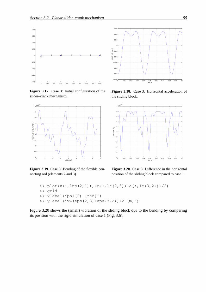
Section 3.2. Planar slider–crank mechanism 55
0 0.05 0.1 0.15 0.2 0.25 0.3 0.35 0.4 0.45-0.2
-0.15
-0.1
-0.05
0
0.05
0.1
0.15
0.2
1 2 3 1 3 6 8
Figure 3.17. Case 3: Initial configuration of theslider–crank mechanism.
0 0.01 0.02 0.03 0.04 0.05 0.06 0.07 0.08 0.09 0.1−6000
−5000
−4000
−3000
−2000
−1000
0
1000
2000
3000
time [s]
(d/d
t)2 x
(8)
[m/s
2 ]
Figure 3.18. Case 3: Horizontal acceleration ofthe sliding block.
0 2 4 6 8 10 12 14 16−4
−3
−2
−1
0
1
2
3
4
5x 10
−3
phi(2) [rad]
v=(e
ps(2
,3)+
eps(
3,2)
)/2
[m]
Figure 3.19.Case 3: Bending of the flexible con-necting rod (elements 2 and 3).
0 0.01 0.02 0.03 0.04 0.05 0.06 0.07 0.08 0.09 0.1−18
−16
−14
−12
−10
−8
−6
−4
−2
0
2x 10
−5
time [s]
x(8)
−x0
(6)
[m]
Figure 3.20. Case 3: Difference in the horizontalposition of the sliding block compared to case 1.
>> plot(x(:,lnp(2,1)),(e(:,le(2,3))+e(:,le(3,2)))/2)>> grid>> xlabel(’phi(2) [rad]’)>> ylabel(’v=(eps(2,3)+eps(3,2))/2 [m]’)
Figure 3.20 shows the (small) vibration of the sliding blockdue to the bending by comparingits position with the rigid simulation of case 1 (Fig. 3.6).

56 Chapter 3. Examples
Nodal points for the planar slider-crank mechanismnode 1 node 2 node 3 node 4,5,7 node 6node 8 node 9
node type T R T R T T Rx-coordinate 0 0.15 0.45 0.30y-coordinate 0 0 0 0BC-typex 1 2 2 2BC-typey 1 2 1 2BC-typeφ 3 2 2φ0 0ω0 = φ 150ω 0forces/moment 0 0 0 0 0 0 0mass/inertia 0 0 0 0 0.033 0 0
T=translational, R=rotational, BC=boundary condition
The numbers of the BC-type refers to the numbers of the groups mentioned on page 16.
Elements for the planar slider-crank mechanismelement 1 element 2element 2a, 3
element type beam beam beamT-nodes 1, 3 3, 6 3, 8 / 8, 6R-nodes 2, 4 5, 7 5, 9 / 9, 7typee1 1 1 1typee2 1 1 4(e2)0 0(e2)0 0typee3 1 1 4mass per length 0.2225 0.2225 0.2225EA 5.65 · 106 5.65 · 106 5.65 · 106
EI 13.4 13.4 13.4damping 0 0 0
T=translational, R=rotational

Section 3.3. Cardan-joint mechanism 57
3.3 Cardan-joint mechanism
In section 11.1 of the lecture notes [1] a cardan joint is described. Cardan joints, also knownas Hooke’s joints, have been used as a shaft coupling in a widerange of machinery, whichincludes locomotive as well as automotive drive lines. A drive line connected by a Cardan jointmay exhibit torsional oscillations due to fluctuating angular velocity ratios inherent in suchsystems.
e(1)1
e(2)1
e(3)1
e(4)1
(a) (b)
Figure 3.21.Schematic of Cardan joint system.
Figure 3.21a shows a one-degree of freedom shaft system incorporating a Cardan joint. TheCardan joint is modelled by four spatial hinge elements as shown in Figure 3.21b. The ro-tating shaft axes having an angular misalignment ofβ = 45 is driven at a constant angularspeede(1) = Ωin. The quantitiese(1) ande(4) represent the input and output angles of the hinge
elements m1 and m4 , respectively.The essential behaviour of the joint can be simulated with the following input file(cardansimp.dat ):
HINGE 1 1 2 -1. 0. 0.HINGE 2 2 3 0. -1. 0.HINGE 3 3 4 0. 0. -1.HINGE 4 4 5 0.707 -0.707 0.
FIX 1FIX 5INPUTE 1 1RLSE 2 1RLSE 3 1RLSE 4 1
END HALT
INPUTE 1 1 0. 6.28 0.TIMESTEP 1.0 100
END END

58 Chapter 3. Examples
Note that in the initial configuration, the input shaft is rotated by a right angle with respect tothe configuration in Figure 3.21.However, the visualization of this simulation is quite poor. This can be improved by addingsome beams to the input and output rotational nodes numbers 2and 4, respectively. The com-plete input file (cardan.dat ) becomes:
HINGE 1 1 2 -1. 0. 0.HINGE 2 2 3 0. -1. 0.HINGE 3 3 4 0. 0. -1.HINGE 4 4 5 0.707 -0.707 0.
BEAM 5 6 2 7 8 0. 1. 0.BEAM 6 7 8 9 10 0. 1. 0.BEAM 7 6 4 11 12 0.707 0.707 0.BEAM 8 11 12 13 14 0.707 0.707 0.
FIX 1FIX 5FIX 6
X 6 0. 0. 0.X 7 1. 0. 0.X 9 1. 0. 0.15X 11 -0.707 0.707 0.X 13 -0.707 0.707 0.15
INPUTE 1 1
RLSE 2 1RLSE 3 1RLSE 4 1
ENDHALT
INPUTE 1 1 0. 6.28 0.
TIMESTEP 1.0 100
ENDEND
The initial configuration of this mechanism is shown in Fig. 3.22. Figures 3.23, 3.24 and 3.25show the zeroth, first and second order geometric transfer functions from inpute(1)
1 to outpute(4)1 , respectively. TheMATLAB commands to plot these data are:
>> plot(e(:,le(1,1)),e(:,le(1,1)), e(:,le(1,1)),e(:,le(4,1)))

Section 3.3. Cardan-joint mechanism 59
−0.8
−0.6
−0.4
−0.2
0
0.2
0.4
0.6
0.8
1
0
0.2
0.4
0.6
0.8
−0.1
0
0.1
Figure 3.22. Initial configuration of the cardanjoint.
0 1 2 3 4 5 60
1
2
3
4
5
6
e1(1) [rad]
e 4(1) [r
ad]
Figure 3.23. Zeroth order geometric transferfunction for the cardan joint.
0 1 2 3 4 5 60.7
0.8
0.9
1
1.1
1.2
1.3
1.4
1.5
e1(1) [rad]
DF
(e1(1
) )
Figure 3.24. First order geometric transfer func-tion for the cardan joint.
0 1 2 3 4 5 6−0.8
−0.6
−0.4
−0.2
0
0.2
0.4
0.6
0.8
e1(1) [rad]
D2 F
(e1(1
) )
Figure 3.25. Second order geometric transferfunction for the cardan joint.
>> grid>> xlabel(’e_1ˆ(1) [rad]’)>> ylabel(’e_4ˆ(1) [rad]’)>>>> plot(e(:,le(1,1)),ed(:,le(4,1))./ed(:,le(1,1)))>> grid>> xlabel(’e_1ˆ(1) [rad]’)>> ylabel(’DF(e_1ˆ(1))’)>>>> plot(e(:,le(1,1)),edd(:,le(4,1))./(ed(:,le(1,1)).ˆ2))>> grid>> xlabel(’e_1ˆ(1) [rad]’)>> ylabel(’Dˆ2F(e_1ˆ(1))’)

60 Chapter 3. Examples
3.4 Planar four-bar mechanism
In examples 5.7.1 and 12.4.1 of the lecture notes [1] the planar four-bar mechanism of Fig. 3.26is analysed analytically. The mechanism has one degree of freedom. The mechanism is mod-elled by four rigid truss elements, denoted by 1, 2, 4 and 5, which are joined together at theirnodal points to form a rhombus. As Fig. 3.26 implies, these four bars are set at right angles
x
y
~1
~2 ~3
~4m
m1 m2
m3
m4 m5
g
k
Figure 3.26.Four-bar mechanism.
to one another. The diagonal element 3 represents a spring with stiffnessk = EA/l0. A con-centrated massm is attached to node 4. The deformation parametere3 has been chosen as thegeneralized coordinate. The equation of motion is
me3 +√
2m(e3)2 + ke3 = mg . (3.1)
Using the coefficient matrices from the lecture notes, the linearized equation of motion is
mδe3 + 2√
2me3δe3 + (k −√
2mg + 2√
2me3 + 5m(e3)2)δe3 = 0 . (3.2)
These results can also be obtained numerically from aSPACAR analysis. E.g. with numericalvalues form = 1, g = 10 andk = 1 and initial conditionse3 = 0 ande3 = 1 the accelerationis according to Eq. (3.1)e3 = 10 −
√2 = 8.59. A SPACAR input file (fourbar.dat ) for this
case is:
PLTRUSS 1 1 2PLTRUSS 2 1 3PLTRUSS 3 2 3PLTRUSS 4 2 4PLTRUSS 5 3 4
X 1 0. 0.

Section 3.4. Planar four-bar mechanism 61
X 2 -0.7071 0.7071X 3 0.7071 0.7071X 4 0. 1.4142
FIX 1FIX 4 1DYNE 3 1
ENDHALT
XM 4 1.XF 4 0. -10.ESTIFF 3 1.4142STARTDE 3 1 0. 1.
ENDEND
In a MATLAB session we get (the literal text of the session is modified somewhat to get a morecompact presentation):
>> spacar(1,’fourbar’)>> e(le(3,1))ans = 0
>> ed(le(3,1))ans = 1
>> edd(le(3,1))ans = 8.5858
Substituting the numerical values of the parameters into the linearized equation of motionEq. (3.2) gives
δe3 + 2√
2δe3 + (1 − 10√
2 + 2√
2(10 −√
2) + 5)δe3 = 0 , (3.3)
or
δe3 + 2.83 δe3 + 16.14 δe3 = 0 . (3.4)
The stiffness term is a combination of
K0 = k = 1
G0 =√
2ke3 = 0
N 0 =√
2g + e3)2 − k/m e3 = 15.14
(3.5)
where the solution of Eq. 3.1
e3 = g −√
2(e3)2 − k/m e3 (3.6)
has been used. In aMATLAB session we get:

62 Chapter 3. Examples
>> spacar(4,’fourbar’)>> m0m0 = 1.0000
>> c0c0 = 2.8285
>> k0k0 = 1
>> n0n0 = 15.1423
>> g0g0 = 0

Section 3.5. Rotating mass–spring system 63
3.5 Rotating mass–spring system
Figure 3.27.Rotating mass–spring system.
Consider the system shown in Fig. 3.27. A smooth horizontal tube containing massesm1
and m2 connected with springsk1 = EA1/l1 and k2 = EA2/l2 is mounted on a rotatingshaft. The shaft rotates at constant angular speedφ. The unstretched lengths of the springs aredenoted byl1 and l2. The equations of motion in terms of the generalized coordinatesr1 andr2 are
[
m1 00 m2
] [
r1
r2
]
=
[
m1φ2r1 − k1(r1 − l1) + k2(r2 − r1 − l2)
m2φ2r2 − k2(r2 − r1 − l2)
]
(3.7)
The stationary solution(r01, r02) is obtained by substitutingr1 = r2 = r1 = r2 = 0
[
k1 + k2 − m1φ2 −k2
−k2 k2 − m2φ2
] [
r01
r02
]
=
[
k1l1 − k2l2k2l2
]
, (3.8)
from which the stationary configuration(r01, r02) is obtained analytically as
r01 =−(m2k1l1 − m2k2l2)φ
2 + k1k2l1
m1m2φ4 − (k2m2 + k2m1 + k1m2)φ2 + k1k2
(3.9)
r02 =−m1φ
2k2l2 + k1k2(l1 + l2)
m1m2φ4 − (k2m2 + k2m1 + k1m2)φ2 + k1k2
(3.10)
This result can also be obtained numerically from a SPACAR analysis. E.g. with the followingnumerical values:
l1 = 0.10 m k1 = 1.3 kN/ml2 = 0.15 m k2 = 0.7 kN/m
m1 = 0.80 kg φ = 10 rad/sm2 = 0.50 kg
A SPACAR input file (massspring.dat ) describing this case is:

64 Chapter 3. Examples
PLBEAM 1 1 2 3 4PLBEAM 2 3 4 5 6PLTRUSS 3 1 5
X 1 0. 0.X 3 0.1 0.X 5 0.25 0.
FIX 1
INPUTX 2 1DYNE 1 1DYNE 3 1
RLSE 2 1
ENDHALT
XM 2 1.XM 3 0.8XM 5 0.5
ESTIFF 1 130.ESTIFF 2 105.
INPUTX 2 1 0.0 10.0
ENDEND
In a MATLAB session we find for the stationary configuration(r01) and(r02) in agreement withEqs. (3.9) and (3.10):
>> spacar(7,’massspring’)>> x(lnp(3,1))
ans = 0.1184
>> x(lnp(5,1))
ans = 0.2891
The linearized equations of motion in terms of the dynamic degrees of freedom are:
[
m1 00 m2
] [
δr1
δr2
]
+
[
k1 + k2 − m1φ2 −k2
−k2 k2 − m2φ2
] [
δr1
δr2
]
=
[
00
]
(3.11)

Section 3.5. Rotating mass–spring system 65
The associated frequency equation is given by:
det
(
− ωi2
[
m1 00 m2
]
+
[
k1 + k2 − m1φ2 −k2
−k2 k2 − m2φ2
])
= 0, (3.12)
where the quantitiesωi are the natural frequencies of the system. In a MATLAB session weobtain:
>> spacar(7,’massspring’)>> m0
m0 =
0.8000 0 0 0.5000
>> k0
k0 =
2000 -700 -700 700
>> n0
n0 =
-80.0000 0 -0.0000 -50.0000
The complex eigenvalues and associated eigenvectors can befound in the log file:
Complex eigenvalues and normalised eigenvectors of the sta te-spacesystem matrixNotation (real : imaginary)Eigenvalue numbers 1 to 4( 0.00000E+00 : +/-5.55511E+01) ( 0.00000E+00 : +/-2.47806 E+01)Eigenvector numbers 1 to 4( 0.0141650 : 0.0000000) ( 0.0177403 : 0.0000000)( -0.0111041 : 0.0000000) ( 0.0362089 : 0.0000000)( 0.0000000 : +/-0.7868804) ( 0.0000000 : +/-0.4396164)( 0.0000000 : -/+0.6168430) ( 0.0000000 : +/-0.8972801)
From the eigenvalues numbers in this table we findω1 = 24.78 rad/s andω2 = 55.55 rad/s.

66 Chapter 3. Examples
3.6 Cantilever beam in Euler buckling
F
l
1 23 4
6521
Figure 3.28.Cantilever beam loaded axially by a forceF at the free end.
Consider a slender cantilever beam or column, with suppressed rotation of the free end, loadedaxially by a forceF . The smallest load that produces buckling is called the critical or Euler loadFcr. For a load equal to or greater than the critical load, the beam is unstable. The bent shapeshown represents the buckling mode. Euler’s theoretical buckling load for the above beam endconditions isFth = π2EI/l2, whereEI is the flexural rigidity andl the length of the beam.This result can also be obtained numerically from a SPACAR analysis, e.g. with the followingnumerical values,l = 1, EI = 1, F0 = 1. The beam is modelled by two equal planar beamelements as shown in Figure 3.28. A SPACAR input file (column2.dat ) for this case is:
PLBEAM 1 1 2 3 4PLBEAM 2 3 4 5 6
X 1 0.0 0.0X 3 0.5 0.0X 5 1.0 0.0
FIX 1FIX 2FIX 6
DYNX 3 2DYNX 4 1DYNX 5 2RLSE 1 2 3RLSE 2 2 3
ENDHALT
EM 1 1.EM 2 1.

Section 3.6. Cantilever beam in Euler buckling 67
ESTIFF 1 0. 1.ESTIFF 2 0. 1.
XF 5 -1.0 0.0
ENDEND
In a MATLAB session we obtain:
>> spacar(8,’column2’)>> edit column2.log
Load multipliers and normalized buckling modesLoad multiplier no 1 to 3
9.94384680E+00 4.00000000E+01 1.28722820E+02Buckling mode nro 1 to 3
0.2596610869 -1.0000000000 -0.05190563010.8141747968 0.0000000000 0.99324167640.5193221738 0.0000000000 -0.1038112603
Hence, we find a load multiplierλ1 = Fcr/F0 = 9.944. SinceF0 = 1 we have Fcr/Fth =9.944/π2 = 1.0075.

68 Chapter 3. Examples
3.7 Cantilever beam subject to concentrated end force
1 2 3 54
F
l
Figure 3.29.Cantilever beam loaded by a concentrated force at the free end.
Consider a slender cantilever beam with a circular cross-section of diameterd = 1 cm andlength l = 10 m. The material properties for this example areEI = 102 Nm2. The beamis subdivided into5 planar finite elements as shown in Fig. 3.29. A point forceF of 14 N isapplied along the vertical axis at the free end of the beam. Itgenerates an elastic deformationas shown in the figure. The deformation is reached in ten stepsof loading. For each step theresidual vector converges in4 Newton–Raphson iterations with an accuracy equal to0.5E − 6.A SPACAR input file (plbeam5.dat ) for this case is:
PLBEAM 1 1 2 3 4PLBEAM 2 3 4 5 6PLBEAM 3 5 6 7 8PLBEAM 4 7 8 9 10PLBEAM 5 9 10 11 12
X 1 0. 0.X 3 1.666 0.X 5 3.333 0.

Section 3.7. Cantilever beam subject to concentrated end force 69
X 7 5. 0.X 9 6.666 0.X 11 10.00 0.
FIX 1FIX 2
DYNE 1 2 3DYNE 2 2 3DYNE 3 2 3DYNE 4 2 3DYNE 5 2 3
ENDHALT
EM 1 1.EM 2 1.EM 3 1.EM 4 1.EM 5 1.
ESTIFF 1 0.0 102.0ESTIFF 2 0.0 102.0ESTIFF 3 0.0 102.0ESTIFF 4 0.0 102.0ESTIFF 5 0.0 102.0
XF 11 0.0 -14
ENDEND
In a MATLAB session we get:
>> spacar(8,’plbeam5’)
>> x(lnp(11,1))ans =
3.6808 (theoretically, 3.8109)
>> x(lnp(11,2))ans =
-8.4897 (theoretically, -8.4044)
>> xcompl(lnp(11,1))ans =

70 Chapter 3. Examples
0.4859 (undeformed configuration, 0.)
>> xcompl(lnp(11,2))ans =
0.0633 (undeformed configuration, 3.268)
To show the usefulness ofSPAVISUAL the first three free vibration modes (no external loads)and buckling modes (axially loaded by an end force) are displayed for the cantilever beam ofthis example in figures 3.30 to 3.35.
Figure 3.30. First vibration mode for a cantileverbeam with 5 elements,ω1 = 0.355131 rad/s (the-oretically,0.355100 rad/s).
Figure 3.31. First buckling mode for a cantileverbeam with 5 elements,Fcr1 = 2.516776 N (theo-retically,2.516749 N).
Figure 3.32. Second vibration mode for a can-tilever beam with 5 elements,ω2 = 2.2266 rad/s(theoretically,2.22537 rad/s).
Figure 3.33. Second buckling mode for a can-tilever beam with 5 elements,Fcr2 = 22.715 N(theoretically,22.651 N).
Figure 3.34.Third vibration mode for a cantileverbeam with 5 elements,ω3 = 6.25198 rad/s (theo-retically,6.23111 rad/s).
Figure 3.35.Third buckling mode for a cantileverbeam with 5 elements,Fcr3 = 64.798 N (theoreti-cally, 62.919 N).

Section 3.8. Short beam 71
3.8 Short beam
F
y
h
l
Figure 3.36.Short Timoshenko beam loaded in shear.
In this example the influence of shear deformation on the behaviour of short beams is studied.A square plate is loaded in shear in its plane as shown in Figure 3.36. The beam has unit height,h, length,l, and Young’s modulus,E, and a small unit width,t. With Poisson’s ratioν = 0.27,the shear correction value isk = 10(1 + ν)/(12 + 11ν) = 0.8484. The deflection, if sheardeflection is taken into account, is
y =Fl3
12EI+
2(1 + ν)Fl
kEth(3.13)
with I = th3/12. So the compliance is
y
F=
l3
12EI+
2(1 + ν)l
kEth= 1 +
2(1 + ν)
k= 3.9940. (3.14)
The moment of inertia per unit of length isJ = ρth3/12.An input file in which the beam is modelled by two planar beams of equal length (shear2.dat )in this case is:
PLBEAM 1 1 2 3 4PLBEAM 2 3 4 5 6
X 1 0.0 0.0X 3 0.5 0.0X 5 1.0 0.0
FIX 1FIX 2FIX 6FIX 5 1RLSE 1RLSE 2DYNX 3

72 Chapter 3. Examples
DYNX 4DYNX 5 2
ENDHALT
EM 1 1.0 0.0833333333EM 2 1.0 0.0833333333ESTIFF 1 1.0 0.0833333333 0.2495ESTIFF 2 1.0 0.0833333333 0.2495
ITERSTEP 10 1 0.000000000001
ENDEND
In a MATLAB session, the compliances and eigenfrequencies can be foundas follows
>> spacar(8,’shear2’)>> xcompl(lnp(5,2))ans =
3.9940>> spacar(7,’shear2’)>> type shear2.log
...
Eigenvalue numbers 5 to 8( 0.00000E+00 : +/-2.54107E+00) ( 0.00000E+00 : +/-7.95645E-01)Eigenvector numbers 5 to 8( 0.0000000 : 0.0000000) ( 0.0000000 : 0.0000000)( -0.1544078 : 0.0000000) ( 0.4065978 : 0.0000000)( 0.2825588 : 0.0000000) ( 0.2566711 : 0.0000000)( 0.1744141 : 0.0000000) ( 0.6173727 : 0.0000000)( 0.0000000 : 0.0000000) ( 0.0000000 : 0.0000000)( 0.0000000 : -/+0.3923612) ( 0.0000000 : +/-0.3235074)( 0.0000000 : +/-0.7180016) ( 0.0000000 : +/-0.2042190)( 0.0000000 : +/-0.4431985) ( 0.0000000 : +/-0.4912094)
...
The compliance based on thin plate theory is3.8822 m/N, so the approximation with a shortbeam overrates the compliance by about 3%. If the shear flexibility were nor included, thecompliance would be1.0 m/N.The lowest numerical eigenfrequency,ω1 = 0.795645 rad/s, compares well with a value fromplate theory,ω1,pl = 0.7987 rad/s. If shear flexibility nor rotational inertia is included, the firstnumerical eigenfrequency is1.6168 rad/s.

Section 3.9. Lateral buckling of cantilever beam 73
3.9 Lateral buckling of cantilever beam
In this example lateral buckling is considered of a cantilever beam with a narrow rectangularcross-section which is loaded by a transverse forceFkipp at its free end in the direction of thelarger flexural rigidity. The theoretical buckling load isFth = 4.013
√(EISt)/l
2, whereEI isthe smaller flexural rigidity,St the torsional rigidity andl the length of the beam. For numericalanalysis, the beam is divided into four equal spatial beam elements in which the second-orderterms in the bending deformations are included in the analysis.In a MATLAB session we get:
>>spacar(8,’lateral4’)>>spavisual(’lateral4’)
An input file (lateral4.dat ) describing this case is:
BEAM 1 1 2 3 4 0. 1. 0.BEAM 2 3 4 5 6 0. 1. 0.BEAM 3 5 6 7 8 0. 1. 0.BEAM 4 7 8 9 10 0. 1. 0.
X 1 0.00 0.00 0.00X 3 0.25 0.00 0.00X 5 0.50 0.00 0.00X 7 0.75 0.00 0.00X 9 1.00 0.00 0.00
DYNE 1 2 5 6DYNE 2 2 5 6DYNE 3 2 5 6DYNE 4 2 5 6
FIX 1FIX 2
OUTLEVEL 0 1
ENDHALT
EM 1 1.0 0.0033EM 2 1.0 0.0033EM 3 1.0 0.0033EM 4 1.0 0.0033
ESTIFF 1 0.0 2.0 0.0 1.0ESTIFF 2 0.0 2.0 0.0 1.0ESTIFF 3 0.0 2.0 0.0 1.0ESTIFF 4 0.0 2.0 0.0 1.0

74 Chapter 3. Examples
XF 9 0.0 0.0 -1.0
ENDEND
VISUALIZATIONBUCKLINGMODE 1TRANSPERANCY 0.9BEAMVIS 0.01 0.1LIGHT 1STEPLINE 0.01ENLARGEFACTOR 0.04
The 3D-visualization of this file is presented in figure 3.37.The buckling load found is5.7619 N,whereas the theoretical value is5.6752 N. If the warping is constrained at the clamped end, thefirst element is effectively shorter for torsion by a distance b
√
(1 + ν)/24, whereb is the heightof the beam, hereb = 0.2 m, andν is Poisson’s ratio, hereν = 0. The torsional stiffness of thefirst beam element now increases with a factorl/(l− b
√
2/3) = 1.19517. The input line for thestiffness of the first beam element now becomes
ESTIFF 1 0.0 2.39034 0.0 1.0
The critical load is now increased to6.1694 N.

Section 3.9. Lateral buckling of cantilever beam 75
F
Figure 3.37.Cantilever beam lateral buckling (buckling mode 1).

76 Chapter 3. Examples
3.10 State-variable and output equations
y
x
b1 m2 k2
k5
1 2
3
5
7 9
l4
l3
1 2
3
4
5
Figure 3.38.Lever system.
Find the state-space-variable and output equations for thesystem shown in Fig. 3.38.The input is the displacementδx7 of the left end of springk2 = EA2/l2; it affects the massm2
through springk5 = EA5/l5 and the lever, which is modelled by the planar beam elements3and4. The lever has a fixed pivot at node5 and is assumed to be massless yet rigid. Its angularorientation is small so that only horizontal motion need be considered. We will selectδx2 andδx2 as state variables, withδx7 being the input and reaction forceδfx
5 as output. With thesedefinitions the state variable and output equations are then:
[
δx2
δv2
]
=
[
0 1−k2/m2 −b1/m2
]
︸ ︷︷ ︸
A
[
δx2
δx2
]
+
[
0−(k2/m2)(l4/l3)
]
︸ ︷︷ ︸
B
[
δx7]
(3.15)
[
δfx5]
=[
−k2(1 + l3/l4) 0]
︸ ︷︷ ︸
C
[
δx2
δx2
]
+[
−k2l3/l4(1 + l3/l4)]
︸ ︷︷ ︸
D
[
δx7]
, (3.16)
which have the desired form. These results can also be obtained numerically from a SPACARanalysis. E.g. with numerical values form2 = 1, b1 = EdA1/l1 = 5, k2 = k5 = 1000 andl4/l3 = 2. A SPACAR input file (lever.dat ) for this case is:
PLTRUSS 1 1 2PLTRUSS 2 2 3PLBEAM 3 3 4 5 6PLBEAM 4 5 6 7 8PLTRUSS 5 7 9
X 1 0.0 0.0
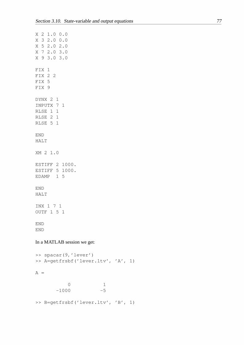
Section 3.10. State-variable and output equations 77
X 2 1.0 0.0X 3 2.0 0.0X 5 2.0 2.0X 7 2.0 3.0X 9 3.0 3.0
FIX 1FIX 2 2FIX 5FIX 9
DYNX 2 1INPUTX 7 1RLSE 1 1RLSE 2 1RLSE 5 1
ENDHALT
XM 2 1.0
ESTIFF 2 1000.ESTIFF 5 1000.EDAMP 1 5
ENDHALT
INX 1 7 1OUTF 1 5 1
ENDEND
In a MATLAB session we get:
>> spacar(9,’lever’)>> A=getfrsbf(’lever.ltv’, ’A’, 1)
A =
0 1-1000 -5
>> B=getfrsbf(’lever.ltv’, ’B’, 1)

78 Chapter 3. Examples
B =
0-2000
>> C=getfrsbf(’lever.ltv’, ’C’, 1)
C =
-3000 0
>> D=getfrsbf(’lever.ltv’, ’D’, 1)
D =
-6000
The state-space matrices can also be obtained with the commandgetss(’lever’) . A Bodediagram (Figure 3.39) can be made by the command
>> bode(getss(’lever’))
0
10
20
30
40
50
60
70
80
90
100
Mag
nitu
de (
dB)
10−1
100
101
102
103
180
225
270
315
360
Pha
se (
deg)
Bode Diagram
Frequency (rad/sec)
Figure 3.39.Bode diagram for the lever system.

Section 3.11. Rigid spatial manipulator mechanism 79
3.11 Rigid spatial manipulator mechanism
Figure 3.40 gives an example of a simplified manipulator. Theprescribed motion of the end-effectorC is represented by the coordinatesxC , yC andzC as functions of time.
x
y
z
I
II
B
C
1, 2
3
4 5
t
v
1.76 m/s
0.0 0.2 0.4 1.0 1.2 1.4
Figure 3.40. Spatial manipulator mechanism, trajectory and velocity profile of the end-effector.
The end-effector must follow the straight trajectory from point I to point II. Three trajectoriesare distinguished: Initially the manipulator is at rest for0.2 s. Next, during 1.0 s, the mo-tion is carried out according to the velocity profile in Fig. 3.40 with constant acceleration anddeceleration during the first and final 0.2 s. Finally the manipulator is at rest again.The motion of manipulator is determined by the rotation of three hinges. Hinge 1 enablesrotations about thez-axis, while hinge 2 enables motions perpendicular to thexy-plane. Hinge 3takes care of motions in the same plane wherein hinge 2 is active. The hinges are driven byinternal actuators. For control purposes we assume that sensors are available that measure therotations and the speed of rotation of the hinges.The manipulator consists of two beams, elements 4 and 5, which are equal in length:l4 =l5 = 0.7 m. The distributed mass per length isρ4 = 4 kg/m for element 4 andρ5 = 2 kg/m forelement 5. The concentrated masses in nodesB andC are10 kg and30 kg respectively. Theeffect of gravity is accounted for by applying external forcesmig in negativez-direction, whereg = 10 m/s2.
Inverse dynamics problem
First the inverse dynamics problem is analysed. Figure 3.44shows the velocity components ofthe end-effector that are computed for the trajectory defined in the input file. The position andacceleration components of the end-effector are shown Fig.3.43 and Fig. 3.45, respectively.The following input file (robotinv.dat ) is used (SPACARmode=2):

80 Chapter 3. Examples
HINGE 1 1 2 0 0 1HINGE 2 2 3 0 -1 0BEAM 4 4 3 5 6 0 1 0HINGE 3 6 7 0 -1 0BEAM 5 5 7 8 9 0 1 0
X 4 0. 0. 0.X 5 0.268 0. 0.6467X 8 0.536 0. 0.
FIX 1FIX 4INPUTX 8 1INPUTX 8 2INPUTX 8 3RLSE 1 1RLSE 2 1RLSE 3 1
ENDHALT
XM 5 10.XM 8 30.EM 4 4.EM 5 2.XF 1 0. 0. -14.XF 5 0. 0. -121.XF 8 0. 0. -307.
ENDHALT
TRAJECT 1TRANS 8 0.536 0. 0.TRTIME 0.2 20TRAJECT 2TRANS 8 0. 1.3 0.TRVMAX 8 0.2 1.76TRFRONT 8 0.TRTIME 1.0 100
TRAJECT 3TRANS 8 0. 1.3 0.TRTIME 0.2 20
NOMS 1 1 1NOMS 2 2 1NOMS 3 3 1
REFE 1 1 1REFE 2 2 1REFE 3 3 1REFEP 4 1 1REFEP 5 2 1REFEP 6 3 1REFEDP 7 1 1REFEDP 8 2 1REFEDP 9 3 1REFX 10 8 1REFX 11 8 2REFX 12 8 3REFXP 13 8 1REFXP 14 8 2REFXP 15 8 3
ENDEND
VISUALIZATIONBEAMVIS 0.01 0.01HINGEVIS 1 0.01 0.03HINGEVIS 2 0.01 0.03HINGEVIS 3 0.01 0.03LIGHT 1TRANSPARENCY 0.6TRAJECT 1TRAJECTNODE 8
The inverse dynamics analysis yields the stresses that haveto be applied at the hinges andthe deformations of the hinges. Fig. 3.42 shows the stresses. Figures 3.46 and 3.47 showthe deformations which are the relative rotations of the hinges, and the first time derivatives,respectively. Clearly, to accomplish the quite simple trajectory of the end-effector of this non-

Section 3.11. Rigid spatial manipulator mechanism 81
Figure 3.41. SPAVISUAL output for the spatial manipulator mechanism.
linear mechanism rather complicated functions for the rotation of the hinges are needed.Note that the input file defines the inputs and outputs that will be used in aSIMULINK simu-lation. The nominal inputs are computed to accomplish the deformations of the hinges. Theoutputs include the six sensor signals with the rotations and the speeds of rotation of the hinges.Nine more outputs are defined to obtain extra information on the performance of the manipula-tor: the acceleration of the rotation of the hinges and position and velocity of the end-effector.At the end of the file visualization settings forSPAVISUAL are defined. In figure 3.41 the outputof SPAVISUAL is presented.

82 Chapter 3. Examples
0 0.2 0.4 0.6 0.8 1 1.2 1.4−200
−100
0
100
200
300
400
500
600
time [s]
u0(1
), u
0(2)
, u0(
3) [N
/m]
Figure 3.42. Stresses to be applied at the hinges(u0).
0 0.2 0.4 0.6 0.8 1 1.2 1.40
0.2
0.4
0.6
0.8
1
1.2
1.4
time [s]
x,y,
z(8)
[m]
Figure 3.43. Position coordinates of the end-effector.
0 0.2 0.4 0.6 0.8 1 1.2 1.4−1
−0.5
0
0.5
1
1.5
2
time [s]
(d/d
t) x
,y,z
(8)
[m/s
]
Figure 3.44. Velocity components of the end-effector.
0 0.2 0.4 0.6 0.8 1 1.2 1.4−10
−8
−6
−4
−2
0
2
4
6
8
10
time [s]
(d/d
t)2 x
,y,z
(8)
[m/s
2 ]
Figure 3.45.Acceleration components of the end-effector.
0 0.2 0.4 0.6 0.8 1 1.2 1.4−1
−0.5
0
0.5
1
1.5
2
time [s]
e1(1
),e1
(2),
e1(3
) [r
ad]
Figure 3.46. Deformations (relative rotations) ofhinges 1, 2 and 3.
0 0.2 0.4 0.6 0.8 1 1.2 1.4−2
−1
0
1
2
3
4
time [s]
(d/d
t) e
1(1)
,e1(
2),e
1(3)
[rad
/s]
Figure 3.47. Velocities of deformation of hinges1, 2 and 3.

Section 3.11. Rigid spatial manipulator mechanism 83
Rotational nodes for the spatial manipulatornode 1 node 2 node 3 node 6 node 7 node 9
type 2 2 2 2 2 2λ0 2 2 2 2 2 2λ1 1 2 2 2 2 2λ2 1 2 2 2 2 2λ3 1 2 2 2 2 2forces 0 0 0 0 0 0I∗∗ 0 0 0 0 0 0
Translational nodes for the spatial manipulatornode 4 node 5 node 8
type 1 1 1x-coordinate 0 0.268 0.536y-coordinate 0 0 0z-coordinate 0 0.647 0BC-typex 1 2 3x0 0.536x0 0BC-typey 1 2 3y0 0y0 0BC-typez 1 2 3z0 0z0 0forcex 0 0 0forcey 0 0 0forcez (∗) -14 -121 -307mass 0 10 30
(∗) including the element masses
Elements for the spatial manipulatorelement 1 element 2 element 3 element 4 element 5
element type hinge hinge hinge beam beamT-nodes 4, 5 5, 8R-nodes 1, 2 2, 3 6, 7 3, 6 7, 9x localy-axis 0 0 0 0 0y localy-axis 0 -1 -1 1 1z local z-axis 1 0 0 0 0typee1 2 2 2 1 1typee2 1 1 1 1 1typee3 1 1 1 1 1typee4 1 1typee5 1 1typee6 1 1
T=translational, R=rotational

84 Chapter 3. Examples
Linearization
In one of the next sections the design of a closed-loop controller for this manipulator will bediscussed. This controller depends on parameters derived from the linearized equations of mo-tion. Therefore, a linearization is needed in terms of the DOFs corresponding to the actuatorjoints. An input file (robotinvlin.dat ) for this analysis (SPACARmode=3) is:
HINGE 1 1 2 0 0 1HINGE 2 2 3 0 -1 0BEAM 4 4 3 5 6 0 1 0HINGE 3 6 7 0 -1 0BEAM 5 5 7 8 9 0 1 0
X 4 0. 0. 0.X 5 0.268 0. 0.6467X 8 0.536 0. 0.
FIX 1FIX 4INPUTE 1 1INPUTE 2 1INPUTE 3 1
ENDHALT
XM 5 10.XM 8 30.EM 4 4.EM 5 2.XF 1 0. 0. -14.XF 5 0. 0. -121.XF 8 0. 0. -307.
ENDHALT
NOMS 1 1 1NOMS 2 2 1NOMS 3 3 1
REFE 1 1 1REFE 2 2 1REFE 3 3 1REFEP 4 1 1REFEP 5 2 1REFEP 6 3 1REFEDP 7 1 1REFEDP 8 2 1REFEDP 9 3 1REFX 10 8 1REFX 11 8 2REFX 12 8 3REFXP 13 8 1REFXP 14 8 2REFXP 15 8 3
ENDEND
Note that the setpoints are read from thesbd data file of which the name is the longest substringof the name of the input file namerobotinvlin . The file from the previous inverse dynamicsrun robotinv is a likely candidate.

Section 3.11. Rigid spatial manipulator mechanism 85
Open-loop simulation
The behaviour of the manipulator mechanism without feed-back control is simulated usingSIMULINK for the open-loop configuration of Fig. 3.48. Two blocks fromthe SPACAR libraryspacar_lib are used to read theSetpoint U0 andReference Y0 data, respectively,from the inverse dynamics run (file namerobotinv ). In this open-loop configuration thenominal input is fed directly into theSPASIM block (also available in the library). In the in-put file robotsim for this block the actual inputs and outputs are identical tothe previouslydefined inputs and outputs.
HINGE 1 1 2 0 0 1HINGE 2 2 3 0 -1 0BEAM 4 4 3 5 6 0 1 0HINGE 3 6 7 0 -1 0BEAM 5 5 7 8 9 0 1 0
X 4 0. 0. 0.X 5 0.268 0. 0.6467X 8 0.536 0. 0.
FIX 1FIX 4DYNE 1 1DYNE 2 1DYNE 3 1
ENDHALT
XM 5 10.XM 8 30.EM 4 4.EM 5 2.XF 1 0. 0. -14.XF 5 0. 0. -121.XF 8 0. 0. -307.
ENDHALT
INPUTS 1 1 1INPUTS 2 2 1INPUTS 3 3 1OUTE 1 1 1OUTE 2 2 1OUTE 3 3 1OUTEP 4 1 1OUTEP 5 2 1OUTEP 6 3 1OUTEDP 7 1 1OUTEDP 8 2 1OUTEDP 9 3 1OUTX 10 8 1OUTX 11 8 2OUTX 12 8 3OUTXP 13 8 1OUTXP 14 8 2OUTXP 15 8 3
ENDEND
The other blocks in the block diagram are standardSIMULINK blocks and are used to export datato workspace and to display results on the screen. The “Selector” blocks select only specifiedcomponents from an input vector. They are e.g. used to selectonly the first three components ofthe output vector (deformations of the hinges) as displaying all components makes the graphsunreadable.SIMULINK ’s ode45 solver is used with a relative tolerance of10−5, an absolute tolerance of10−8 and a maximum time step of0.01 s. With these parameters the simulation of the motionfrom t = 0.0 s to t = 1.5 s is completed after 172 time steps. The size of many time steps is

86 Chapter 3. Examples
yref
Yref To Workspace
y
Y To Workspace
unom
Unom To Workspace
t
Time To Workspace
robotinvlin
Setpoint U0
Selector
Selector Ytip
Selector
Selector Eref
Selector
Selector E
Scope dYtip
Scope Eref
Scope ErobotsimSPASIM
robotinvlin
Reference Y0
1.5
Display Time
Clock
3
3
315
15
15
15
3
15
15
15
15
3
15 3
Figure 3.48. Block diagram for an open-loop simulation of the motion of the manipulatormechanism usingSIMULINK .
0 0.2 0.4 0.6 0.8 1 1.2 1.4−1
−0.5
0
0.5
1
1.5
2
time [s]
e1(1
),e1
(2),
e1(3
) [r
ad]
e(1)1
e(2)1
e(3)1
Figure 3.49. Deformation of the hinges of spatialmanipulator mechanism in an open-loop simula-tion.
0 0.2 0.4 0.6 0.8 1 1.2 1.4−0.2
0
0.2
0.4
0.6
0.8
1
1.2
1.4
time [s]
x,y,
z(8)
[m]
x(8) y(8)
z(8)
Figure 3.50. Position of the end-effector of spa-tial manipulator mechanism in an open-loop sim-ulation.
dictated by the specified maximum value.The results from the simulation are plotted using theMATLAB commands;
>> plot(t,yref(:,1),’r’,t,yref(:,2),’g’,...t,yref(:,3),’b’,t,y(:,1),’r:’,...t,y(:,2),’g:’,t,y(:,3),’b:’)
>> plot(t,yref(:,10),’r’,t,yref(:,11),’g’,...t,yref(:,12),’b’,t,y(:,10),’r:’,...t,y(:,11),’g:’,t,y(:,12),’b:’)
Figures 3.49 and 3.50 show the deformation of the hinges and the position coordinates of theend-effector from this simulation. The solid lines are the reference data (yref ) and the dottedlines are from the actual simulation (y ). Clearly, small errors during the integration lead torelatively large position errors at the end of the motion. The error can be decreased by increasingthe integration accuracy, e.g. by enlarging the number of computed setpoints. More reliableresults can be obtained by applying feedback control, as will be discussed next.
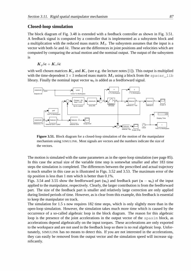
Section 3.11. Rigid spatial manipulator mechanism 87
Closed-loop simulation
The block diagram of Fig. 3.48 is extended with a feedback controller as shown in Fig. 3.51.A feedback signal is computed by a controller that is implemented as a subsystem block anda multiplication with the reduced mass matrixM 0. The subsystem assumes that the input is avector with bothδe andδe. These are the differences in joint positions and velocities which arecomputed by comparing the actual motion and the nominal output. The output of the subsystemis
Kpδe + Kvδe
with well chosen matricesKp andKv (see e.g. the lecture notes [1]). This output is multipliedwith the time-dependent3× 3 reduced mass matrixM 0 using a block from thespacar_liblibrary. Finally the nominal input vectoru0 is added as a feedforward signal.
robotinvlin
times M0
yref
Yref To Workspace
y
Y To Workspace
unom
Unom To Workspace
u
U To Workspace
t
Time To Workspace
robotinvlin
Setpoint U0
Selector
Selector Ytip
Selector
Selector Eref + Edref
Selector
Selector Eref
Selector
Selector E + Ed
Selector
Selector E
Scope dYtip
Scope Eref
Scope ErobotsimSPASIM
robotinvlin
Reference Y0
Omega = 28beta = 0.85
Kp Kv control
1.5
Display Time
Clock
1515
15
15
3
366
6
33
33Unom 3
3
6 3 3
6
6
6
315
1515
15
15
Figure 3.51. Block diagram for a closed-loop simulation of the motion of the manipulatormechanism usingSIMULINK . Most signals are vectors and the numbers indicate the size ofthe vectors.
The motion is simulated with the same parameters as in the open-loop simulation (see page 85).In this case the actual size of the variable time step is somewhat smaller and after 183 timesteps the simulation is completed. The differences betweenthe prescribed and actual trajectoryis much smaller in this case as is illustrated in Figs. 3.52 and 3.53. The maximum error of thetip position is less than 1 mm which is better than 0.1%.Figs. 3.54 and 3.55 show the feedforward part (u0) and feedback part (u − u0) of the inputapplied to the manipulator, respectively. Clearly, the larger contribution is from the feedforwardpart. The size of the feedback part is smaller and relativelylarge correction are only appliedduring limited periods of time. However, as is clear from this example, this feedback is essentialto keep the manipulator on track.The simulation for 1.5 s now requires 182 time steps, which isonly slightly more than in theopen-loop simulation. However, the simulation takes much more time which is caused by theoccurrence of a so-called algebraic loop in the block diagram. The reason for this algebraicloop is the presence of the joint accelerations in the outputvector of thespasim block, asaccelerations depend algebraically on the input torques. These accelerations are only exportedto the workspace and are not used in the feedback loop so thereis no real algebraic loop. Unfor-tunately,SIMULINK has no means to detect this. If you are not interested in the accelerations,they can easily be removed from the output vector and the simulation speed will increase sig-nificantly.

88 Chapter 3. Examples
0 0.2 0.4 0.6 0.8 1 1.2 1.4−2.5
−2
−1.5
−1
−0.5
0
0.5
1
1.5x 10
−3
time [s]
e1(1
)−e1
ref(
1),e
1(2)
−e1
ref(
2),e
1(3)
−e1
ref(
3) [r
ad]
e(1)1 − e
(1)1,ref
e(2)1 − e
(2)1,ref
e(3)1 − e
(3)1,ref
Figure 3.52. Error in the deformation of thehinges of spatial manipulator mechanism in aclosed-loop simulation.
0 0.2 0.4 0.6 0.8 1 1.2 1.4−7
−6
−5
−4
−3
−2
−1
0
1
2
3x 10
−4
time [s]
x−xr
ef,y
−yr
ef,z
−zr
ef(8
) [m
]
x(8) − x(8)ref
y(8) − y(8)ref
z(8) − z(8)ref
Figure 3.53. Position error of the end-effector ofspatial manipulator mechanism in a closed-loopsimulation.
0 0.2 0.4 0.6 0.8 1 1.2 1.4−200
−100
0
100
200
300
400
500
600
time [s]
u0(1
,2,3
) [N
/m]
u(1)0
u(2)0
u(3)0
Figure 3.54. Input applied to the manipulator:feedforward part (u0).
0 0.2 0.4 0.6 0.8 1 1.2 1.4−20
−10
0
10
20
30
40
time [s]
u−u0
(1,2
,3)
[N/m
]
u(1) − u(1)0
u(2) − u(2)0
u(3) − u(3)0
Figure 3.55. Input applied to the manipulator:feedback part (u − u0).

Section 3.12. Flexible spatial manipulator mechanism 89
3.12 Flexible spatial manipulator mechanism
To be added ...

90 Chapter 3. Examples
3.13 Chord-driven underactuated robotic finger
FM
distal phalanx
proximal phalanxfirst pulley
second pulley
third pulley
Figure 3.56.Robotic finger.
In order to illustrate the use of the planar belt/gear element, a model for a chord-driven underac-tuated robotic finger with two phalanges, as in a thumb, is considered; see Fig. 3.56. The distalphalanx can rotate with respect to the proximal phalanx and the proximal phalanx can rotatewith respect to the palm, which is assumed to be immobile. A pulley is rigidly connected tothe distal phalanx, centred at its rotation point, which carries a chord that is slung over a secondpulley centred at the rotation point of the proximal phalanx, but free to rotate. The chord isfinally attached to a third pulley, which is driven by a motor.The finger is underactuated, forit has two degrees of freedom, but a single motor. The degreesof freedom are chosen as therelative rotation angle between the two phalanges and the rotation angle of the motor pulley.A forceF = 10 N acts near the tip of the finger, which is balanced by a momentM = 1.5 Nmdelivered by the motor. Owing to the choice of the dimensionsof the radii of the pulleys andthe lengths of the phalanges, this is an equilibrium position.
1 2 3
45
6
FM
y
x
Figure 3.57.Finite element model for the robotic finger.
The finite element model is shown in Fig. 3.57. The input file,finger.dat , is
PLBEAM 1 1 2 3 4PLTOR 2 4 5PLBEAM 3 3 5 6 7PLBELT 4 8 9 1 10 -0.015 -0.015

Section 3.13. Chord-driven underactuated robotic finger 91
PLBELT 5 1 10 3 5 -0.015 -0.009PLRBEAM 6 6 7 11FIX 1 1 2FIX 8 1 2DYNX 9 1DYNE 2 1X 1 0 0X 3 0.06 0.0X 6 0.15 0.0X 8 0 -0.06X 11 0.15 -0.015ENDHALTEM 3 1.0EM 5 1.0STARTDX 9 1 0.0 0.0STARTDE 2 1 0.0 0.0XF 11 0.0 10.0XF 9 -1.5TIMESTEP 0.2 100ENDENDVISUALIZATIONVIBRATIONMODE 1ENLARGEFACTOR 0.2
By running SPACAR with mode=7, it can be checked that the initial position is indeed anequilibrium position, but it is unstable. One mode has an eigenvalue equal to zero, and inthe corresponding mode shape, the distal phalanx remains horizontal. The other mode has anexponentially increasing or decaying motion and is shown inFigure 3.58. (Note that the currentversion ofSPAVISUAL does not draw the pulleys.) A simulation with an initial perturbation,specified by
STARTDX 9 1 0.001 0.04STARTDE 2 1 0.004 0.16
shows this unstable behaviour. Note that the initial perturbation is approximately in the directionof the eigenvector corresponding to the unstable eigenvalue.
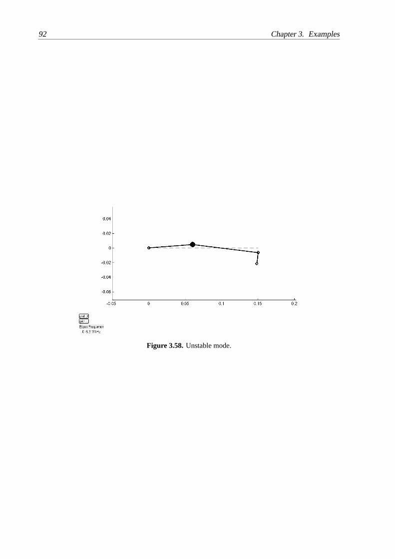
92 Chapter 3. Examples
Figure 3.58.Unstable mode.
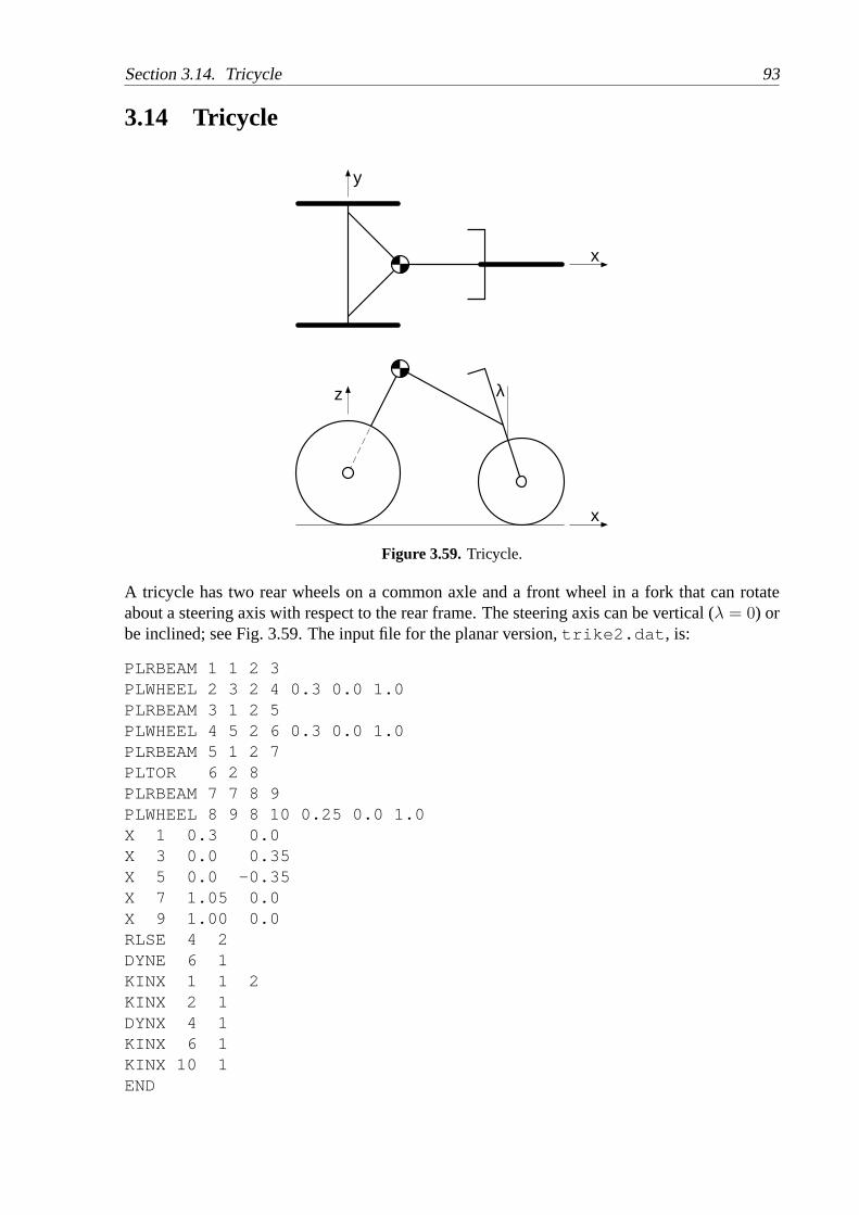
Section 3.14. Tricycle 93
3.14 Tricycle
x
y
x
z λ
Figure 3.59.Tricycle.
A tricycle has two rear wheels on a common axle and a front wheel in a fork that can rotateabout a steering axis with respect to the rear frame. The steering axis can be vertical (λ = 0) orbe inclined; see Fig. 3.59. The input file for the planar version, trike2.dat , is:
PLRBEAM 1 1 2 3PLWHEEL 2 3 2 4 0.3 0.0 1.0PLRBEAM 3 1 2 5PLWHEEL 4 5 2 6 0.3 0.0 1.0PLRBEAM 5 1 2 7PLTOR 6 2 8PLRBEAM 7 7 8 9PLWHEEL 8 9 8 10 0.25 0.0 1.0X 1 0.3 0.0X 3 0.0 0.35X 5 0.0 -0.35X 7 1.05 0.0X 9 1.00 0.0RLSE 4 2DYNE 6 1KINX 1 1 2KINX 2 1DYNX 4 1KINX 6 1KINX 10 1END

94 Chapter 3. Examples
HALTXM 1 80.0XM 2 5.0XM 3 2.0XM 4 0.1XM 5 2.0XM 6 0.1XM 8 0.025XM 9 1.5XM 10 0.05STARTDX 4 1 0.0 10.0STARTDE 6 1 0.5 0.0TIMESTEP 1.0 100ENDEND
The origin of the coordinate system is initially located at the centre of the rear axle, with thex-axis pointing in the forward direction and they-axis pointing to the left. The centre of massof the frame is at a distance of 0.3 m in front of the rear axle. The rear wheels, elements 2 and 4,have a radius of 0.3 m and are connected to the centre of mass ofthe frame by two rigid beams,elements 1 and 3. Another rigid beam, element 5, connects thecentre of mass of the frameto the steering head, where the hinge, element 6, makes the connection to the front fork. Therigid beam 7 represents the rigid connection between the steering head and the the front wheel,element 8, with radius 0.25 m, which is conncted to the front fork. All wheels can rotate freelyabout their spin axis. The frame and the wheels have mass, butthe front fork is assumed to bemassless.The system has two degrees of freedom: the rotation angle of the left rear wheel and the steeringangle are chosen as generalized coordinates. The lateral slip of the right rear wheel is released,because otherwise the system whould be overconstrained. The other five slips at the wheelsare prescribed as zero to impose the non-holonomic constraints of pure rolling. Five kinematiccoordinates are defined as the two position coordinates and the yaw angle for the rear frame andthe two rotation angles at the other wheels. The moments of inertia at the nodes 4, 6 and 10 arethe moments of inertia about the spin axes of the wheels.The stationary motion and the linearized equations can be found by runningSPACAR withmode=7. It appears that there are seven eigenvalues equal to zero, with eigenvectors whichcorrespond to the three rotations of the wheels and the two positions and yaw angle of the rearframe, and a change in the forward velocity. The other two eigenvalues are real and negative,corresponding to exponentially decaying motion. A simulation can be made withmode=1.A three-dimensional model of the same tricycle is (filetrike3v.dat )
RBEAM 1 1 2 3 0.0 1.0 0.0HINGE 2 2 4 0.0 1.0 0.0WHEEL 3 3 4 5 0.0 1.0 0.0RBEAM 4 1 2 6 0.0 1.0 0.0HINGE 5 2 7 0.0 1.0 0.0WHEEL 6 6 7 8 0.0 1.0 0.0RBEAM 7 1 2 9 0.0 1.0 0.0HINGE 8 2 10 0.0 0.0 1.0

Section 3.14. Tricycle 95
RBEAM 9 9 10 11 0.0 1.0 0.0HINGE 10 10 12 0.0 1.0 0.0WHEEL 11 11 12 13 0.0 1.0 0.0HINGE 12 14 2 0.0 0.0 1.0X 1 0.3 0.0 0.9X 3 0.0 0.35 0.3X 5 0.0 0.35 0.0X 6 0.0 -0.35 0.3X 8 0.0 -0.35 0.0X 9 1.05 0.0 0.3X 11 1.00 0.0 0.25X 13 1.00 0.0 0.0FIX 14RLSE 12 2 3RLSE 6 6DYNE 2 1DYNE 8 1KINE 5 1KINE 10 1KINE 12 1KINX 1 1KINX 1 2ENDHALTGRAVITY 0.0 0.0 -9.81XM 1 80.0XM 2 2.0 0.0 0.0 3.0 0.0 5.0XM 3 2.0XM 4 0.0 0.0 0.0 0.1 0.0 0.0XM 6 2.0XM 7 0.0 0.0 0.0 0.1 0.0 0.0XM 11 1.5XM 12 0.025 0.0 0.0 0.05 0.0 0.025STARTDE 2 1 0.0 10.0STARTDE 8 1 -0.5 0.0TIMESTEP 1.0 100ENDEND
Note that hinges (elements 2, 5 and 10) are used to connect thewheels to the rigid beams andan additional hinge, element 12, is introduced in order to make the yaw angle available. Withmode=7, the same eigenvalues are found as for the planar model. If variables are saved fromthe run with the planar model, it will be seen that the resultsof a simulation are very nearly thesame. The three-dimensional model has the advantage that the normal forces at the wheels arecalculated, which are the first components of the stress of the wheel elements (Fig 3.60):
>> plot(time,sig(:,le(3,1)),’k-’,time,sig(:,le(6,1)),’k:’, ...time,sig(:,le(11,1)),’k--’); grid on

96 Chapter 3. Examples
0 0.1 0.2 0.3 0.4 0.5 0.6 0.7 0.8 0.9 1−600
−500
−400
−300
−200
−100
0
time [s]
norm
al fo
rce
[N]
Figure 3.60. Normal forces at road contact points. The fully drawn line is for the left rearwheel, the dotted line for the right rear wheel and the dashed line for the front wheel.
>> xlabel(’time [s]’)>> ylabel(’normal force [N]’)
It is seen that all forces are negative, which means that the normal force is compressive, as itshould be. The normal force in the right rear wheel is initially much higher than the corre-sponding force at the left rear wheel. Because the wheel planes remain perpendicular to theroad surface, the third components of the stresses are also equal to the normal force at the road.Lateral forces are in the second components, as well as in thesixth in a scaled version. Thefourth components of the stresses are zero, as they should be. The fifth components representscaled longitudinal tyre forces at the contact points.A model with an inclined steering axis, as shown in Fig. 3.59,is in the input filetrike3i.dat ,which differs fromtrike3v.dat in the definition of the hinge at the steering head, element 8,and the position of node 9,
...
HINGE 8 2 10 -0.30901699437495 0.0 0.95105651629515
...
X 9 0.96 0.0 0.3
...

Section 3.14. Tricycle 97
0 0.1 0.2 0.3 0.4 0.5 0.6 0.7 0.8 0.9 1−600
−500
−400
−300
−200
−100
0
time [s]
norm
al fo
rce
[N]
Figure 3.61. Normal forces at road contact points. The fully drawn line is for the left rearwheel, the dotted line for the right rear wheel and the dashed line for the front wheel.
Note that for this case, the normal force in the right rear wheel is initially just compressive(Figure 3.61), so for a slightly higher speed, the wheel would lose contact with the ground.This loss of contact cannot directly be included in the model. The front wheel no longer staysperpendicular to the road surface, so the first and third stress components are no longer equal.Morreover, the rotation angle of the hinge with element number 12 is not exactly equal to theyaw angle in this case.

98 Chapter 3. Examples
3.15 Screw motion
x
z
12
3
x
y
12
4
Figure 3.62.Screw moving a flexible beam.
We consider the kinematic model of a screw pushing against a flexible beam. In the modelshown in Fig. 3.62, element 1 is a screw element fixed at one endand conected to a hingeelement, element 2, which is free to rotate and is rigidly connect to a flexible beam element,element 3, which is fixed at its other end. A rigid beam element, element 4, is only includedto show the rotation of the screw. The screw as well as the flexible beam have a length of 1 m.The pitch of the screw is 1 cm/radian. The input file isscrew.dat ,
SCREW 1 1 2 3 4 1 0 0 0.01X 1 0.0 0.0 0.0X 3 1.0 0.0 0.0FIX 1FIX 2HINGE 2 4 5 1 0 0DYNE 2 1BEAM 3 6 7 3 5 1.0 0.0 0.0RLSE 3X 6 1.0 0.0 -1.0FIX 6FIX 7RBEAM 4 1 2 3 0.0 1.0 0.0RLSE 4RBEAM 5 3 4 8 1.0 0.0 0.0X 8 1.0 0.2 0.0INPUTE 1 1END

Section 3.15. Screw motion 99
HALTEM 3 1.0ESTIFF 3 1000.0 1.5 100.0 1.0EDAMP 3 1000.0 0.015 0.1 0.01INPUTE 1 1 0.0 1.0 0.0STARTDE 2 1 0.0 -1.0TIMESTEP 10 200ENDENDTIMESTEP 1.0 100ENDEND
The screw is driven over an angle of 10 radians in 10 seconds. The moment to drive to screwand the normal force in the flexible beam (bothσ1) are shown in Fig 3.63. This figure wasgenerated by the commands
>> plot(time,100 * sig(:,le(1,1)),’k--’,time,sig(:,le(3,1)),’k-’); grid on>> xlabel(’time [s]’)>> ylabel(’normal force [N] and driving torque [N cm]’)
As the distance between the end points of the flexible beam increases, the normal force increasesin approximately a quadratic way.
0 1 2 3 4 5 6 7 8 9 10−4
−2
0
2
4
6
8
time [s]
norm
al fo
rce
[N] a
nd d
rivin
g to
rque
[N c
m]
Figure 3.63. Normal force in the flexible beam 3 (fully drawn) and the negative drivingtorque of the screw (dashed).

100 Chapter 3. Examples

A
SPACAR installation
Prerequisites
Before installingSPACAR on a computer system it is advisable to check that the system issuitable of running the software and to haveMATLAB installed.This SPACAR version has been developed and tested withMATLAB 7.0.4 andSIMULINK 6.2(Release 14SP2). It is expected to work with any modern version of MATLAB /SIMULINK sinceR12, but in case of problems we can offer only limited support.The system requirements depend heavily on the version ofMATLAB you are using. Consult theaccompanying Installation Guide or check The Mathworks. You may expect thatSPACARwillrun on any Microsoft 32-bit Windows PC on whichMATLAB /SIMULINK are running. Only thebase systems ofMATLAB andSIMULINK are required to runSPACAR, but additional toolboxeslike the Control System Toolbox may be helpful to develop and analyse control systems.The installation ofSPACARuses less than 4 MB extra disk space.TheSPACARfiles are stored in ZIP-archives or, in Microsoft Windows XP,a compressed folder.In Windows XP you can easily open such archives, but of courseyou may chose to use yourfavourite unzipper. The ZIP-archives can be downloaded fromhttp://www.wa.ctw.utwente.nl/Software/SPACAR/ .In addition to the software there is a ZIP-archive with the data files that are used for the examplesin Chapter 3.
Installation
First of all, you should create a subdirectory e.g.\Matlab\Toolbox\Spacar . Next, youextract the files from theSPACAR software ZIP-archivespacar2007_bin.zip into thissubdirectory. There are three types of files:
• Files with the extension.dll are the actual executables of theSPACAR package. Theoriginal SPACAR-code (not provided) is written inC and FORTRAN77, compiled andlinked into so-called MEX-modules, that are executables for use within the MATLAB-environment. The following files must exist:
101

102 Appendix A. SPACAR installation
checksbf.dll combsbd.dll getfrsbf.dll loadsbd.dllloadsbm.dll ltv.dll mrltv.dll repinsbf.dllspacar.dll spacntrl.dll spasim.dll
• Files with extension.m are theMATLAB -files necessary to use theSPACARprogram. Thefollowing file must exist:
spadraw.m
Other.m-files provide help text for the MEX-modules. These files are:
checksbf.m combsbd.m getfrsbf.m getss.mloadsbd.m loadsbm.m ltv.m mrltv.mrepinsbf.m spacar.m spacntrl.m spasim.m
• Files with extension.mdl areSIMULINK models. There is only one file which is actuallya library from which theSPACARmodules for use inSIMULINK can be copied:
spacar_lib.mdl
The (optional) data files fromspadata.zip can be extracted in a separate working directory.The files in theSPACARsubdirectory should be in theMATLAB path whenMATLAB is running.There are two ways to accomplish this:
1. Make sure that theSPACAR subdirectory is the local directory. You can verify this bytypingpwd. If necessary, change your local directory by typing
cd \Matlab\Toolbox\Spacar
or whatever directory you chose to store your files.
2. Another possibility is to change the settings of theMATLAB environment by adding theSPACARsubdirectory to theMATLAB path. This modification is either temporary or per-manent. The path can be modified from the pulldown menu withFile |Set Path... ,or by using theMATLAB commandspath or addpath .
Now you are ready to runSPACAR in MATLAB andSIMULINK .

B
SPACAR error messages
An analysis withSPACARin MATLAB or a simulation withSPASIM in SIMULINK can suffer fromerrors. These errors can be divided into fatal errors that cause an immediate terminations andless severe errors which may report unexpected conditions in thelog file, while the calculationcontinues.Most fatal error have a clear error message:
• SPACAR requires 2 or 3 input arguments ,SPACAR requires no output argument ,CCONST must be 1 x N or N x 1 vector ,CCONST contains too many parameters ,MODE has an invalid value andFILENAME contains illegal charactersindicate an incorrect call ofSPACAR from MATLAB . The last error can also occur inSPASIM (SIMULINK ).
• Wrong number of input arguments ,Flag must be a scalar variable ,Too many output arguments ,Time must be a scalar variable ,State vector of wrong size ,Input vector of wrong size andNot a valid flag numberindicate an incorrect call ofSPASIM from SIMULINK and should not occur during normaloperation.
• ERROR opening file ... means thatSPACAR can not open the specified file foroutput.
• ERROR opening existing file ... means that a file from a previous run is notfound.
• ERROR in subroutine DINVOE is caused by an error in the dynamics input, seeSect. 2.3.
103

104 Appendix B. SPACAR error messages
• PREPTR: Illegal velocity profile is reported when no valid velocity profilecan be determined.
• Can not determine valid and existing input file names from... means that nomode=2 output data file with extensionsbd matching the current(mode=3) data file can be found.
• Mechanisms are different ,Configuration mismatch LE andConfiguration mismatch LNParise from an error during the comparison between a the configuration used in a (previous)mode=2 run and the currentmode=3 run.
• ERROR in subroutine ORDE0: IFLAG = 2 andERROR in subroutine ORDE0: No convergenceindicate problems with the zeroth order iteration. InSPASIM this may be avoided bysetting or decreasing the maximum time step ofSIMULINK ’s solver.
• ERROR in subroutine SOLDYN is usually caused by a singular mass matrix.
• PRPARE: NUMBER OF NXC NOT EQUAL TO NEO+NEMis caused by an ill-definedmechanism.
• ERROR in subroutine PRPARE: Too many ... means that the mechanismthat is defined is too large to be handled by theSPACAR version you are using, see Ta-ble 1.1 on page 10. Simplify the mechanism or contact the authors.
The messages written to thelog file may be self-explanatory, but also a somewhat crypticmessages “ERROR OR POSSIBLE ERROR CODED: <code> ITEM: <number>” canoccur. The<code> is related to a procedure in the software. Typical examples are:
• INVOERi input for the kinematics (Sect. 2.2).
• SINVOERi input for the inverse dynamics (setpoint generation) (Sect. 2.4).
• LIMVOEi input for the linearization (Sect. 2.5).
• SIMVOEi input for the non-linear simulation of manipulator control(Sect. 2.6).
• PREPTR.. trajectory data processing.
Note that errors in the input file are often reported one line later than the actual error position.

C
MATLAB tutorial
C.1 Basic MATLAB graphics commands
MATLAB provides a variety of functions for displaying data. This section describes some ofthese functions. For a complete survey of graphics functions available inMATLAB we refer tothe officialMATLAB documentation [2] or to the online help utility.
Elementary plotting functions
The following list summarizes the functions that produce basic line plots of data. These func-tions differ only in the way they scale the plot axes. Each accepts input in the form of vectorsor matrices and automatically scales the axes to accommodate the input data.
• plot – creates a plot of vectors or columns of matrices.
• loglog – creates a plot using logarithmic scales for both axes.
• semilogx – creates a plot using a logarithmic scale for thex-axis and a linear scale forthey-axis.
• semilogy – creates a plot using a linear scale for thex-axis and a logarithmic scale forthey-axis.
You can add titles, axis labels, grid lines, and text to your graph using
• title – adds a title to the graph.
• xlabel – adds a label to thex-axis.
• ylabel – adds a label to they-axis.
• text – displays a text string at a specified location.
• gtext – places text on the graph using the mouse.
• grid – turns on/off grid lines.
105

106 Appendix C. MATLAB tutorial
Creating a plot
If y is a vector,plot(y) produces a linear graph of the elements ofy versus the index of theelements ofy . If you specify two vectors as arguments,plot(x,y) produces a graph ofyversusx .
Line styles, markers, and color
You can pass a character string as an argument to theplot function in order to specify variousline styles, plot symbols, and colors. In the statement
plot(x,y,s)s is a 1-, 2-, or 3-character string (delineated by single quotes) constructed from the charactersin the following table:
Symbol Color Symbol Linestyley yellow . pointm magenta o circlec cyan x x-markr red + plusg green * starb blue - solidw white : dottedk black -. dashdot
-- dashed
For example,plot(x,y,’c+’) plots a cyan plus symbol at each data point.If you do not specify a color, theplot function automatically uses the colors in the above table.For one line, the default is yellow because this is the most visible color on a black background.For multiple lines, theplot function cycles through the first six colors in the table.
Adding lines to an existing graph
You can add lines to an existing graph using thehold command. When you sethold to on ,MATLAB does not remove the existing lines; instead it adds the new lines to the current axes. Itmay, however, rescale the axes if the new data fall outside the range of the previous data. Forexample:
plot(f1)hold onplot(f2,’--’)plot(f3,’-.’)hold off
These statements produce a graph displaying three plots.

Appendix C. MATLAB tutorial 107
Creating hardcopy of MATLAB figures
You can make a hardcopy of a figure from the figure’s menu (File |Print... ) or by pressingCtrl+P . Output to several graphics formats can be carried out as well (File |Export... ).Alternatively,MATLAB ’s print command can be used at theMATLAB command prompt. E.g.you can generate PostScript output of the contents the current MATLAB figure window. Theprint command sends the output directly to your default printer orwrites it to the specifiedfile, if you supply a filename. You can also specify the type of PostScript file. Supported typesinclude
• PostScript (-dps )
• Color PostScript (-dpsc )
• Encapsulated PostScript (-deps )
• Encapsulated color PostScript (-depsc )
For example, the statement
print dataplot -deps
saves the contents of the current figure window as Encapsulated PostScript in the file calleddataplot.eps . Depending on yourMATLAB installation other graphics formats are sup-ported, tryhelp print .
C.2 Quitting and saving the workspace
To quit MATLAB , typequit or exit . Terminating aMATLAB session deletes the variables inthe workspace. Before quitting, you can save the workspace for later use by typing
saveThis command saves all variables in a file on disk namedmatlab.mat . The next timeMAT-LAB is invoked, you can executeload to restore the workspace frommatlab.mat .You can usesave andload with other filenames, or to save only selected variables. Thecom-mandsave temp stores the current variables in the file namedtemp.mat . The command
save temp Xsaves only variableX, while
save temp X,Y,ZsavesX, Y, andZ.load temp retrieves all the variables from the file namedtemp.mat .

108 Appendix C. MATLAB tutorial

References
[1] Jonker, J. B.,Dynamics of Machines and Mechanisms, A Finite Element Approach,Lecture notes, Department of Mechanical Engineering, University of Twente, vakcode113130, October 2001.
[2] The Math Works Inc.,Getting Started withMATLAB , version 7, Revised forMATLAB 7.1(Release 14SP3), September 2005.
[3] The Math Works Inc.,SIMULINK — Getting Started, version 6, New forSIMULINK 6.3(Release 14SP3), September 2005.
[4] SAM, Version 4.2, 5.0 or 5.1, ARTAS - Engineering Software, The Netherlands,http://www.artas.nl/ , 2001–2005.
[5] Cowper, G. R., “The shear coefficient in Timoshenko’s beam theory”, ASME Journal ofApplied Mechanics33 (1966), pp. 335–340.
109