Sovereign Spreads: Global Risk Aversion, Contagion or Fundamentals?

Carlos Caceres, Vincenzo Guzzo and

Miguel Segoviano1

1 Director General of Risk Analysis and Quantitative Methodologies, Comisiόn Nacional Bancaria y de Valores (Mexican Financial Authority).

WP/10/120

© 2010 International Monetary Fund WP/10/120 IMF Working Paper Monetary and Capital Markets Department

Sovereign Spreads: Global Risk Aversion, Contagion or Fundamentals? 2

Prepared by Carlos Caceres, Vincenzo Guzzo and Miguel Segoviano

Authorized for distribution by Udaibir S. Das

May 2010

Abstract

This Working Paper should not be reported as representing the views of the IMF. The views expressed in this Working Paper are those of the author(s) and do not necessarily represent those of the IMF or IMF policy. Working Papers describe research in progress by the author(s) and are published to elicit comments and to further debate.

Over the past year, euro area sovereign spreads have exhibited an unprecedented degree of volatility. This paper explores how much of these large movements reflected shifts in (i) global risk aversion (ii) country-specific risks, directly from worsening fundamentals, or indirectly from spillovers originating in other sovereigns. The analysis shows that earlier in the crisis, the surge in global risk aversion was a significant factor influencing sovereign spreads, while recently country-specific factors have started playing a more important role. The perceived source of contagion itself has changed: previously, it could be found among those sovereigns hit hard by the financial crisis, such as Austria, the Netherlands, and Ireland, whereas lately the countries putting pressure on euro area government bonds have been primarily Greece, Portugal, and Spain, as the emphasis has shifted towards short-term refinancing risk and long-term fiscal sustainability. The paper concludes that debt sustainability and appropriate management of sovereign balance sheets are necessary conditions for preventing sovereign risk from feeding back into broader financial stability concerns. JEL Classification Numbers: E43, E44, G01, G10.

Keywords: Sovereign spreads; contagion; market price of risk; fiscal policy.

Author’s E-Mail Address: ccaceres@imf.org, vguzzo@imf.org,

2Without any implication, we would like to thank Peter Dattels, Joseph Di Censo, Julio Escolano, Raphael Espinoza, Geoffrey Heenan, Matthew Jones, Laura Kodres, Christian Mulder, Robert Sheehy, and Mark Stone for constructive comments and discussions. We would also like to thank Julia Guerreiro for excellent research assistance. Any errors are solely the authors’ responsibility.

msegoviano@cnbv.gob.mx

2 Contents Page

I. INTRODUCTION ..................................................................................................................3

II. DATA AND CONSTRUCTION OF THE MAIN VARIABLES ........................................5 A. THE INDEX OF GLOBAL RISK AVERSION (IGRA) .......................................................7 B. THE SPILLOVER COEFFICIENT (SC) ............................................................................9

III. ESTIMATION METHODOLOGY AND MAIN RESULTS ...........................................12 A. THE ESTIMATION MODEL .........................................................................................12 B. ESTIMATION RESULTS ..............................................................................................13

IV. DISCUSSION ....................................................................................................................13

V. POSSIBLE EXTENSIONS ................................................................................................15

VI. CONCLUSIONS ...............................................................................................................16 Figures 1. Euro area Sovereign 10-Year Swap Spreads .........................................................................6 2. Index of Global Risk Aversion (IGRA) ...............................................................................10 3. The Sources of Contagion: Systemic Outbreak vs. Sovereign Risk Phase ..........................15

Boxes 1. The Market Price of Risk and Global Risk Aversion ............................................................8 2. The CIMDO Methodology ..................................................................................................11

References ................................................................................................................................28

Annexes Annex I.....................................................................................................................................18 Annex II ...................................................................................................................................20 Annex III ..................................................................................................................................22 Annex IV ..................................................................................................................................26 Annex V ...................................................................................................................................27

3

I. INTRODUCTION

Over the past year, euro area sovereign yields have exhibited an unprecedented degree of volatility. In March 2009 the spread between the yield on a 10-year Greek government bond and the yield on a German Bund of equivalent maturity was as high as 280 basis points (bp). By September 2009 the same spread had dropped below 120 bp. In January 2010, it had climbed back up to over 380 bp. Other government bonds have followed a similar trajectory with volatility being higher among higher-debt, lower-rated sovereigns. Likewise, the credit default swap, in other words the premium investors are willing to pay to insure the same Greek bond against a credit event, during the same period has also moved from a level of around 50 bp, up to almost 300bp, down to 100 bp, and up again to 350 bp.

Movements in government bonds yields can have significant macroeconomic consequences. A rise in sovereign yields tend to be accompanied by a widespread increase in long-term interest rates in the rest of the economy, affecting both investment and consumption decisions. On the fiscal side, higher government bond yields imply higher debt-servicing costs and can significantly raise funding costs. This could also lead to an increase in rollover risk, as debt might have to be refinanced at unusually high cost or, in extreme cases, cannot be rolled over at all. Large increase in government funding costs can thus cause real economic losses, in addition to the purely financial effects of higher interest rates.

As the crisis unfolded, several factors might have affected the valuations of sovereign bonds. First, the global market price for risk went up, as investors sought higher compensation for risk. Deleveraging and balance sheet-constrained investors developed a systemically stronger preference for a few selected assets vis-à-vis riskier instruments. This behavior not only benefited sovereign securities as an asset class at the expense of corporate bonds and other riskier assets, but also introduced a higher degree of differentiation within the sovereign spectrum itself.

Second, as the crisis spread to the public sector and policy authorities stepped in to support troubled financial institutions, probabilities of distress went up across sovereigns. In this context, two distinct channels may be identified: a domestic channel, as fundamentals started deteriorating, and an external channel, as higher probabilities of distress spread among sovereigns. This paper aims to assess to what extent the large fluctuations observed in euro sovereign spreads reflect changes in global risk aversion or they reveal the insurgence of country-specific risk, via worse fundamentals or contagion from other countries.

Some discussion of the existing literature on euro sovereign spreads,3

3 This work focuses on sovereign spreads for advanced markets. Hartelius K. et al (2008) look at the influence of liquidity and fundamentals on sovereign spreads with a focus on emerging markets.

and how this work differs from it, is warranted. The paper by Afonso and Strauch (2004) find that specific policy events in 2002, when the Stability and Growth Pact came under close market scrutiny, had only temporary and limited impact on swap spreads. Using a broader information set with data from before and after the start of EMU, Bernoth, et al (2004) show that yield spreads are affected by international

4 risk factors and reflect positive default as well as liquidity premia. They conclude that the monetary union does not seem to have weakened the disciplinary function of credit markets. Codogno, et al (2003) draw similar conclusions.

Manganelli and Wolswijk (2007) argue that the fact that interest rates are strongly correlated not only to government bond spreads, but also to spreads between corporate and government bonds, suggests that the main driver of these spreads is the level of short-term interest rates. If investors take on more liquidity and credit risk in the government bond market when interest rates are low, spreads will be compressed, thus generating a positive correlation between interest rates and spreads. While one should be wary of the endogeneity embedded in these relationships, their conclusions appear to have been overcome by the recent financial crisis, when spreads kept widening despite historically low interest rates. In a more recent work, Mody (2009) identifies the rescue of Bear Stearns in March 2008 as a turning point with sovereign spreads widening when the prospects of a domestic financial sector worsened.

Explicitly modeling sovereign spreads on measures of global risk aversion and distress dependence is one of the key aspects of this study. Other research papers have attempted to include proxies for global risk aversion in the analysis of sovereign spreads. However, some of these measures tend to be over simplistic and to be affected by a wide range of factors, thus not capturing the specific concept of global risk aversion. For instance, the spreads of US corporate bonds over Treasury bonds,4

Other methods rely on extracting the (unobserved) “risk aversion” component from the actual (observed) sovereign spread series—in other words “filtering.”

which are likely to be affected by a large number of institution-specific or country-specific factors, cannot be considered an exclusive measure of global risk aversion. The main benefit of such proxies is that they are based on observable measures and are therefore readily available.

5

The inclusion of a measure of distress dependence—or a spillover coefficient—is another original twist in this study. In particular, by explicitly differentiating among distress dependence, global risk aversion, and country-specific fundamentals, this analysis can separately identify the effects of each of these factors on sovereign spreads. In fact, the common factor obtained through the use of

Although statistically viable, these measures depend on the adopted data sample, as global risk aversion is assumed to be proxied by the time-varying common factor of the analyzed series. Our measure of global risk aversion is based on the methodology developed in Espinoza and Segoviano (2010). This measure is completely independent of our data sample, and does not change according to which countries are being considered.

4 Used in, e.g., Codogno et al (2003), Schuknecht et al (2010).

5 For example, Geyer et al (2004) extract the common factor embedded in EMU spreads based on the use of a Kalman filter. Sgherri and Zoli (2009) apply a Bayesian filtering technique to extract the time-varying common factor from a non-linear model of the sovereign spreads.

5 filtering techniques mentioned above might be explained by global risk aversion as well as contagion.6

This paper is organized as follows. Section II introduces the dataset and focuses on the construction of the global risk aversion and distress dependence measures. Section III presents the estimation model. Section IV assesses the main findings, whereas Section V extends the analysis to a noneuro area framework. Section VI concludes.

II. DATA AND CONSTRUCTION OF THE MAIN VARIABLES

We measure euro area spreads as spreads of sovereign bond yields to a common numeraire. This is the yield on a 10-year euro swap, in other words, the yield at which one party is willing to pay a fixed rate in order to receive a floating rate from a given counterparty. Typically, the yield on an AAA-rated government bond would trade below the swap yield. In contrast, yields on lower-rated bonds might be above the swap yield as investors demand a higher premium on these riskier assets. The banking crisis and the following interventions of the sovereigns to support financial institutions have significantly altered these relationships.

The resulting data set spans from mid-2005, well ahead of the start of the crisis, through early 2010, for a total of over 1,000 daily observations, encompassing ten euro sovereign markets7. The paths of these spreads since mid 2007 are shown on Figure 1. Four distinct phases can be identified. Between July 2007 and September 2008, a phase which we call financial crisis build-up, most of these spreads remained within a relatively narrow, albeit widening, range. In most cases, sovereign bond yields held or fell further below the swap yield as bank counterparty risk was weighing adversely on swaps. Between October 2008 and March 2009, the systemic outbreak following the collapse of Lehman Brothers, these spreads diverged markedly. With the exception of German Bunds, government bond yields moved sharply above the swap yield, as problems in the banking sector spilled over to sovereign balance sheets.8

6 For instance, one could think of developments in an individual country affecting all other countries in the sample, without any changes in global risk aversion. In that case, the common trend cannot be considered as a measure of global risk aversion, but rather of contagion.

Between April and September 2009, the systemic response phase, spreads converged, although at wider levels. As financial spillovers were contained and systemic risk subsided, all bond yields fell back closer to the level of the swap yield, particularly those which had gone up considerably in the earlier phase. Finally, since October 2009, rising idiosyncratic sovereign risk led to greater differentiation among countries, with the yields on specific government bonds climbing once again to record highs relative to the swap yield.

7 The sample is made of the first 12 countries that joined EMU, excluding Finland and Luxembourg (due to lack of long and reliable CDS spread series).

8 Note that while the EMU sovereign bond market became thinner during the most acute phase of the crisis, it was still liquid enough in the case of these sovereign 10-year benchmarks to materialize in actual trades. Bid-ask spreads were definitely wider and volumes fell, yet to levels high enough to allow this type of analysis.

6

Figure 1. Euro area Sovereign 10-Year Swap Spreads

-1.5

-1.0

-0.5

0.0

0.5

1.0

1.5

2.0

2.5

3.0

3.5

4.0

Euro Area Sovereign 10Y Swap Spreads

GER FRA

ITA SPA

NET BEL

AUT GRE

IRE POR

Financial Crisis Build-Up SystemicOutbreak

SystemicResponse

SovereignRisk

Source: IMF Staff calculations on DataStream and Bloomberg data. In order to address the question of what is driving euro area sovereign spreads, we introduce a dynamic model where each of these spreads is regressed on a number of factors. Namely:

(i) Global Risk Aversion. The price of an asset reflects both market expectations of the asset’s returns and the price of risk, i.e., the price that investors are willing to pay for receiving income in “distressed” states of nature. The Index of Global Risk Aversion (IGRA) typifies the market price of risk. It allows us to extract from asset prices the effects of the price of risk and thus to compute the market’s expectation of the probability of distress. This result is achieved by using the methodology developed in Espinoza and Segoviano (2010) and summarized in Section II.A.

(ii) Contagion, captured by a measure of distress dependence—the Spillover Coefficient (SC)—which characterizes the probability of distress of a country conditional on other countries (in the sample) becoming distressed. This indicator embeds distress dependence across sovereign credit default swaps (CDS) and their changes throughout the economic cycle, reflecting the fact that dependence increases in periods of distress. The SC is based on the methodology developed by Segoviano and Goodhart (2009) and presented in Section II.B.

7 (iii) Country specific fundamentals, identified by each country’s stock of public debt and budget deficit as a share of GDP.9

The inclusion of measures of global risk aversion and contagion in the analysis of sovereign swap spreads represents a novel approach. The IGRA and the SC were developed in order to disentangle the effect of country-specific fundamentals from that of increased market risk aversion or contagion on these spreads. This is a critical step as sovereign bond spreads might well exhibit significant movements without any noticeable change in their fiscal position.

In particular, the SC measure quantifies the distress dependence between the various countries in our sample. This dependence captures the macrofinancial linkages among these countries including trade, capital flows, financial sector linkages, as well as contingent liabilities among sovereigns. This last element is important, as the countries included in the sample belong to a monetary union in which fiscal transfers are (implicitly) absent. Yet the market might attribute a high probability to the event that a country experiencing sovereign distress would be ultimately supported by other countries in the union. The country in distress is effectively considered as a contingent liability for the other countries.

A. The Index of Global Risk Aversion (IGRA)

The credit crisis raised the importance of assessing the underlying dynamics of default probabilities. These probabilities can be estimated by using models of the value of the firm (e.g. the Black-Scholes-Merton model) or by relying on measures of market assessment, such as CDS spreads.

CDS spreads are widely used to generate risk-neutral probabilities of default.10

Espinoza and Segoviano (2010) propose an original method to estimate the market price of risk under stress (see Box 1 for technical details). The market price of risk under stress, in other words the expectation of the market price of risk exceeding a certain threshold, is computed from its two moments: the variance of the market price of risk and its discount factor, which is simply the inverse of the expected market price of risk. The price of risk can be estimated through different

Yet, these spreads, just as any other market risk indicator, are in fact asset prices that depend on global risk aversion as well as idiosyncratic news on the actual probability of default of a specific firm or sovereign. Therefore, it is necessary to strip out the price effect of risk aversion in order to be able to use CDS spreads to compute probabilities of default.

9 The daily series for the fiscal variables where obtained by using a linear interpolation on the underlying quarterly data. This is based on the assumption that these variables tend to explain the low-frequency movements in the swap spreads, with almost no impact on high frequency (daily) variations.

10 These probabilities of default are estimated by dividing the level of the Credit Default Swap (CDS) by its Recovery Rate (R). See Luo (2005).

8

Box 1. The Market Price of Risk and Global Risk Aversion

CDS spreads are asset prices that depend on global risk aversion as well as idiosyncratic news on the actual probability of default of a specific firm. It is therefore necessary to strip out the price effect of risk aversion in order to be able to use CDS spreads to compute probabilities of default. The linear pricing and the risk-neutral pricing formulae (see Cochrane, 2001) state that, if mt+1(s) is the price of a security paying $1 in state s, then the price of an asset paying off an uncertain stream xt+1 next period is:

ft

ttttf

tstttt r

xEsxs

rsxsmsP

+=

+== +

+++++ ∑∑ 1][ˆ

)()(ˆ1

1)()()( 111111 ππ

)(1 st+π is the actual probability of nature that state s occurs and ftr is the risk-free rate. Note

that: )1/(1)(1f

ts

t rsm +=∑ + ) and )()()1()(ˆ 111 smsrs ttf

tt +++ += ππ [3]

is called the risk-neutral probability because it is the probability measure that a risk-neutral investor would need to use, when forming her expectations and computing an NPV consistent with the market price of the asset Pt. Estimating the actual probability of default from a CDS spread-implied risk-neutral probability is equivalent to estimating the market price of risk in the state where the CDS pays off (the distress test). Espinoza and Segoviano (2010) use the conditional expectation formula for normal distributions to estimate

][1)(

][var][][][ 111111t

tttttttttt mmEthresholdmmEdistressmE

ααϕ−+++++ Φ−

+=>= [4]

where ][var/])[( 11 ++−= ttttt mmEthresholdα , ϕ is the normal distribution density function, and

1−Φ is the inverse cumulative distribution function of the normal distribution. ][var 1+tt m is deduced from

the price of risk )var()1( 1++= tf

tm mrλ , which is an important variable in the CAPM literature. In a CAPM, excess returns are equal to the price of risk multiplied by the quantity of risk – the beta of an asset -

since mmif

ti

tt rrE λβ ,1 ][ =−+ . The price of risk can be estimated via the Fama-MacBeth regressions.

Espinoza and Segoviano (2010) suggest a calibration based on the VIX. At any single point in time, the market price of risk under stress (the conditional expectation) is re-calculated since the risk-free rate (the mean) and the price of risk (the variance) are changing. This results in a single measure of the market price of risk under stress, which is the same across all countries11

. The threshold defines the scenario under which the asset is under distress. It can be defined exogenously or it can be chosen, in a more consistent way, such that the probability that the market-price of risk exceeds the threshold is equal to the actual probability of nature:

)var(*]1[][ 1 mmEthreshold tπ−Φ+= − [5] In that case, the nonlinear equations [3], [4] and [5] have to be solved jointly. Espinoza and Segoviano (2010) show that there is a unique solution.

11 In theory, this is based on the assumption of market completeness, which should hold for all the countries. From a practical viewpoint, however, one could price several countries’ assets using a one factor model (for instance, by performing Fama-MacBeth regressions on the sample of stocks in all the countries under consideration).

9 methods. For instance, it can be derived from the VIX12 or from the factors in a Fama-MacBeth regression.13

On average, the actual probability of a CDS pay-off is around 40 percent of the risk-neutral probability of distress. The rest is explained by macroeconomic and financial factors. These factors matter because creditworthiness depends on fundamentals and on the liquidity environment. This percentage has likely declined during the Lehman crisis to around 30 percent, as global risk increased and therefore a larger share of CDS was being driven by the market price of risk.

For this analysis, the IGRA was constructed using the formula:

IGRAt = -(1-PoRt) [1]

where PoRt is the share of the market price of risk in the actual probability of the stress event (as estimated in Espinoza and Segoviano, 2010). This index reflects the market perception of risk14

B. The Spillover Coefficient (SC)

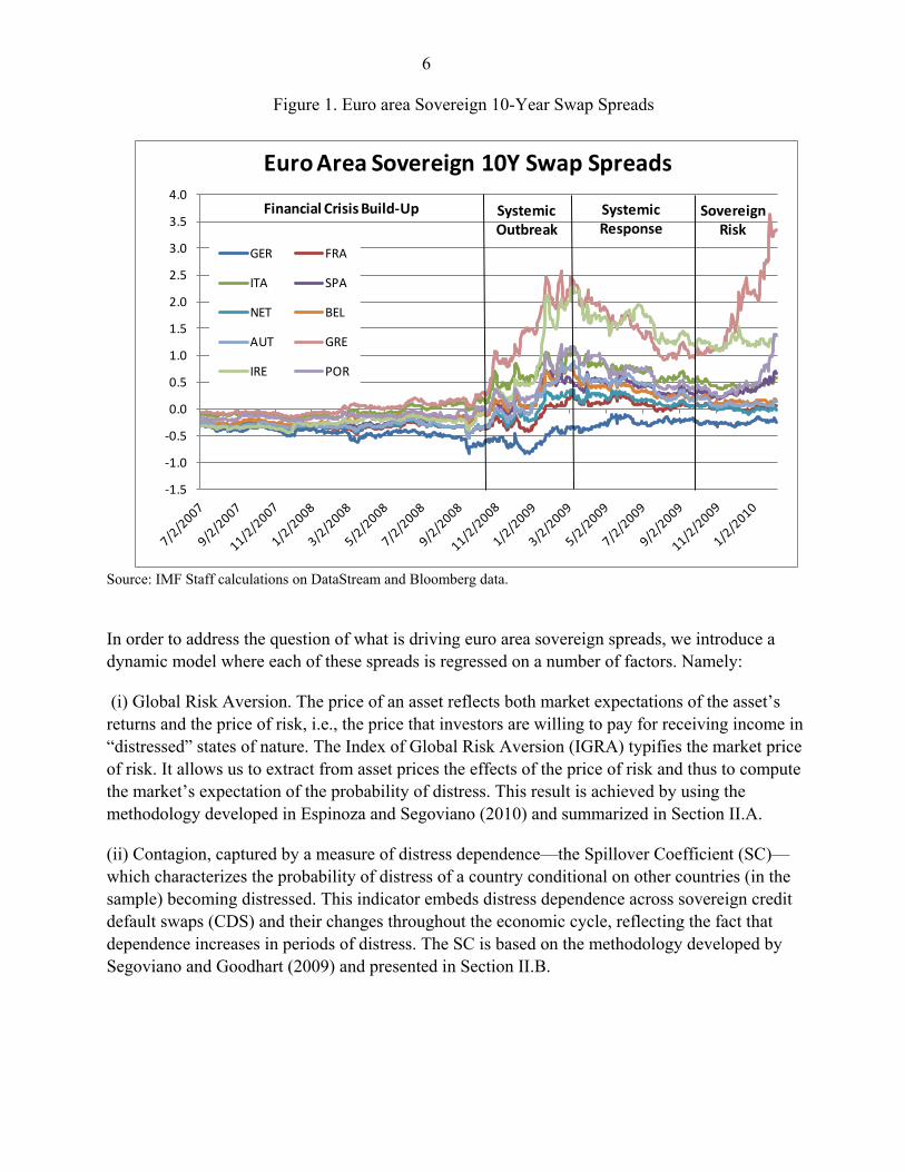
at every point in time, and—as highlighted in Figure 2—it captures the sharp increase in global risk aversion observed after September 2008, followed by a gradual reduction throughout most of 2009.

Contagion plays a crucial role in explaining the behavior of sovereign swap spreads. Hence, we constructed a measure of distress dependence, the SC—in order to quantify the role that contagion plays in the underlying risk of default of a given country. Essentially, the SC characterizes the probability of distress of a country conditional on other countries becoming distressed.

For each country Ai, the SC is computed using the formula:

SC(Ai) = ∑ P(Ai/Aj) · P(Aj) for all j ≠ I [2]

which is essentially the weighted sum of the probability of distress of country Ai given a default in each of the other countries in the sample. This measure of distress dependence is appropriately weighed by the probability of each of these events to occur.

The probability of sovereign distress in country Ai given a default by country Aj, referred here as the probability of Ai given Aj, denoted by P (Ai/Aj), is obtained in three steps:

12 VIX is the Chicago Board Options Exchange Volatility Index, a popular measure of implied volatility of S&P 500 index options.

13 The Fama-MacBeth regression is a method used to estimate parameters for asset pricing models such as the Capital Asset Pricing Model (CAPM).

14 This is a single, exogenously given, measure of global risk aversion, for all the countries included in the sample. Note that Espinoza and Segoviano (2010) estimate this market price of risk using the US Libor OIS rate and the VIX, thus not relying on any country-specific information from the euro area economies (see Box 1 for details).

10

Figure 2. Index of Global Risk Aversion (IGRA)

-0.45

-0.43

-0.41

-0.39

-0.37

-0.35

-0.33

-0.31

Jul-2007 Jan-2008 Jul-2008 Jan-2009 Jul-2009 Jan-2010

Index of Global Risk Aversion

Source: IMF Staff calculations.

(i) The marginal probabilities of default for countries Ai and Aj, P (Ai) and P (Aj) respectively, are extracted from the individual CDS spreads for these countries.15

(ii) Then, the joint probability of default of Ai and Aj, P (Ai, Aj), is obtained using the CIMDO methodology developed by Segoviano (2006) (see Box 2 for technical details). This methodology is used to estimate the multivariate empirical distribution (CIMDO-distribution) that characterizes the probabilities of distress of each of the sovereigns under analysis, their distress dependence, and how such dependence changes along the economic cycle. The CIMDO methodology is a nonparametric methodology, based on the Kullback (1959) cross-entropy approach, which does not impose parametric pre-determined distributional forms; whilst being constrained to characterize the empirical probabilities of distress observed for each institution under analysis (extracted from the CDS spreads). The joint probability of distress of the entire group of sovereigns under analysis and all the pair wise combinations of sovereigns within this group, i.e., P (Ai, Aj), are estimated from the CIMDO-distribution.

(iii) Finally, the conditional probability of default P(Ai/Aj) is obtained by using the Bayes’ law: P(Ai/Aj) = P(Ai,Aj) / P(Aj).

15 We assume a recovery rate of 40% for sovereigns, as commonly used in the literature.

11

Box 2. The CIMDO Methodology

The detailed formulation of CIMDO is presented in Segoviano (2006). CIMDO is based on the Kullback (1959) minimum cross-entropy approach (MXED). For illustration purposes, we focus on a portfolio containing loans contracted by two different classes of borrowers, whose logarithmic returns are characterized by the random variables x and y, where x, y ∈ɭ i s.t.

i=1,..,M. Therefore, the objective function can now be defined as C[p,q]=∫ ∫p(x,y)ln ( , )( , )

p x yq x y

dxdy, where

q(x,y) the is prior distribution and p(x,y) the posterior distribution It is important to point out that the initial hypothesis is taken in accordance with economic intuition (default is triggered by a drop in the firm’s asset value below a threshold value) and with theoretical models (Structural Approach), but not necessarily with empirical observations. Thus, the information provided by the frequencies of default of each type of loan making up the portfolio is of primary importance for the recovery of the posterior distribution. In order to incorporate this information into the recovered posterior density, we formulate moment- consistency constraint equations of the form

( ) ( ), ,( , ) , ( , )x y

d d

x yt tx x

p x y dxdy PoD p x y dydx PoDχ χ∞ ∞

= =∫ ∫ ∫ ∫

where ( , )p x y is the posterior multivariate distribution that represents the unknown to be solved. xtPoD and

ytPoD are the empirically observed probabilities of default (PoDs) for each borrower in the portfolio

and ( ) ( ), ,,x y

d dx xχ χ

∞ ∞ are the indicating functions defined with the default thresholds for each borrower in the

portfolio. In order to ensure that ( , )p x y represents a valid density, the conditions that ( , )p x y ≥0 and the

probability additivity constraint, ∫∫ ( , )p x y dxdy=1, also need to be satisfied. Imposing these constraints on the optimization problem guarantees that the posterior multivariate distribution contains marginal densities that in the region of default are equalized to each of the borrowers’ empirically observed probabilities of default. The CIMDO density is recovered by minimizing the functional

[ ], ( , ) ln ( , ) ( , ) ln ( , )L p q p x y p x y dxdy p x y q x y dxdy= −∫ ∫ ∫ ∫

1 [ , )( , ) x

d

xtx

p x y dxdy PoDλ χ∞

+ − ∫ ∫ 2 [ , )( , ) y

d

ytx

p x y dydx PoDλ χ∞

+ − ∫ ∫

( , ) 1p x y dxdyµ + − ∫ ∫

Where 1 2λ λ represent the Lagrange multipliers of the moment-consistency constraints and represents the Lagrange multiplier of the probability additivity constraint. By using the calculus of variations, the optimization procedure is performed. The optimal solution is represented by the following posterior multivariate density as

{ }, ) , )1 2[ [( , ) ( , ) exp 1 ( ) ( )x y

d dx xp x y q x y µ λ χ λ χ∞ ∞

= − + + +

12 Contrary to simple correlations, or relationships based on the first few moments of different default probability series, the CIMDO methodology enables us to characterize the entire distributional links between these series, i.e., linear (correlations) and nonlinear distress dependence, and their evolution throughout the economic cycle. This reflects the fact that dependence increases in periods of distress. This is a key technical improvement over traditional risk models, which usually account only for linear dependence (correlations) that are assumed to remain constant over the cycle, over a fixed period of time, or over a rolling window of time. Such dependence structure is characterized by a copula function (CIMDO-copula), which changes at each period in time, consistently with changes in the empirically observed distress probabilities.16

III. ESTIMATION METHODOLOGY AND MAIN RESULTS

We heuristically introduce the copula approach to characterize dependence structures of random variables and explain the particular advantages of the CIMDO-copula in Annex I.

A. The Estimation Model

The model used in the analysis of the determinants of sovereign swap spreads is described by the following General Autoregressive Conditional Heteroskedasticity (GARCH(1,1)) specification:

Yt = α Yt-1 + β’Xt + εt [6]

σt2 = ω + θ εt-1

2 + γ σt-12 [7]

where [6] is the mean equation for the swap spread Yt as a function of the explanatory variables stacked in the vector Xt (including a constant term), and an error term εt, with conditional variance σt

2. This conditional variance is given by equation [7] as function of the lag of the squared residual from the mean equation εt-1

2 (the ARCH term), and last period’s variance σt-12 (the GARCH term).

The explanatory variables include the Index of Global Risk Aversion (IGRA), a measure of distress dependence captured by the Spillover Coefficient (SC) and two country-specific fiscal variables, namely the overall balance as percent of GDP and the debt-to-GDP ratio. The lag dependent variable is included in the model to capture the high persistence inherent in the daily time series of the swap spreads.17

The inclusion of measures of risk aversion and distress dependence, the IGRA and the SC, in the regression analysis of the sovereign swap spreads represents an original approach. This step not only enables us to quantify the effect of these two important factors on the dynamics of swap spreads, but it also mitigates the bias in the estimation of the coefficients for the country-specific

16 We heuristically introduce the copula approach to characterize dependence structures of random variables and explain the particular advantages of the CIMDO-copula in Annex I.

17 The presence of the lag dependent variable mitigates the autocorrelation that would otherwise be observed in the residuals from estimating equation [6] without the lag dependent variable.

13 fundamental variables that would otherwise arise from the omission of these two measures in the regression.18

B. Estimation Results

The results from the estimation of the model described by equations [6] and [7] are presented in Table 1 (see Annex II).19

(i) Global risk aversion is generally a positive factor for euro area government bonds, with the notable exception of lower-rated, high-debt countries. When global risk aversion is on the rise, swap spreads widen,

The main findings can be summarized as follows:

20

(ii) Contagion, in contrast, is always negative for government bonds. When the probability of a credit event in a country (given distress in another sovereign issuer) rises, swap spreads tighten, as sovereign bond yields rise closer to the swap yield or move above that level. More importantly, high-debt, lower-rated sovereigns such as Greece or Italy tend to exhibit larger sensitivities as these countries will likely be more vulnerable to even remote probabilities of distress among higher-rated issuers.

as sovereign bond yields fall further below swap yields. As flight-to-quality leads to capital flowing away from risky assets towards government securities, sovereign bonds tend to do better than swaps. In the adopted sample, this is not the case for a high-debt, A-rated issuer that does not benefit from a flight-to-quality effect. As a result, the spreads between AAA-rated country and lower-rated ones tend to widen significantly.

(iii) Fundamentals also exhibit a significant relationship with these spreads. Swap spreads tighten, in other words sovereign bond yields rise versus swap yields when public debts (in percentage of GDP) rise or budget balances deteriorate.

IV. DISCUSSION

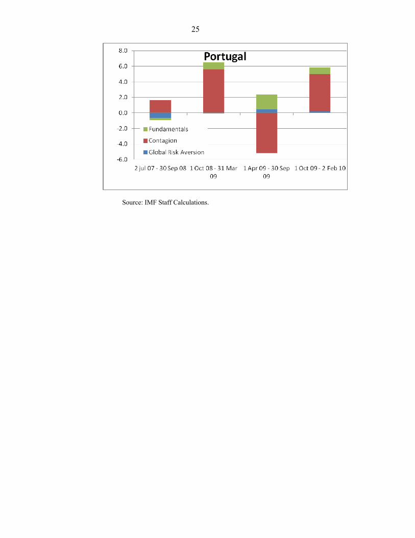
On the back of this analysis, not only we can assess the sign of the impact of the various factors—namely, global risk aversion, contagion, and country-specific fundamentals—on swap spreads, but we can also identify how they contributed to the cumulative changes in spreads. The following stylized conclusions can be drawn for:

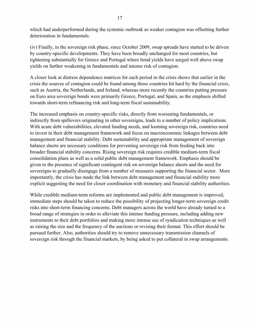
(i) During the financial crisis build-up, between July 2007 and September 2008, German swap spreads widened (i.e., German Bund yields fell relative to swap yields) on the back of global risk aversion, as German securities were benefiting from flight-to-quality flows, and fundamentals, as both the deficit and the debt were still improving (see Figure 4 in Annex III). In contrast, bonds 18 A regression analysis that omits the effect of increased risk aversion or contagion might lead to an overestimation of the effects played by country-specific fundamentals.

19 The estimation of this model for all the countries in the sample was carried out in EViews via Maximum Likelihood Estimation, using the Marquardt Optimization Algorithm.

20 We follow the European market convention for which swap spread tightens (widens) when bond yields rise (fall) versus swap yields, even in those cases where bond yields are actually above swap yields.

14 from peripheral countries saw their yields rising versus swap yields already during this first phase of the crisis as global risk aversion was weighing adversely on these lower-rated issuers.

(ii) During the systemic outbreak, between October 2008 and March 2009, as sovereigns stepped in and supported financial institutions, swap spreads tightened (i.e., government bond yields rose relative to swap yields) across the board, on risk of contagion and fundamentals, which had started deteriorating. Global risk aversion was not playing such a favorable role any longer as crisis-related interventions and fiscal stimulus packages had diluted the perception of sovereigns as a riskless asset class.

(iii) During the systemic response phase, between April 2009 and September 2009, all swap spreads widened (i.e., government bond yields fell back towards swaps), as lower probability of distress in some countries was favorably affecting others. The correction was larger among those bonds such as Italy and Greece which had underperformed during the systemic outbreak as lower contagion was offsetting further deterioration in fundamentals.

(iv) Finally, in the sovereign risk phase, between October 2009 and now, swap spreads have started to be driven by country-specific developments. They have been broadly unchanged for most countries, but tightening substantially for Greece and Portugal where bond yields have surged well above swap yields on further weakening in fundamentals and intense risk of contagion.

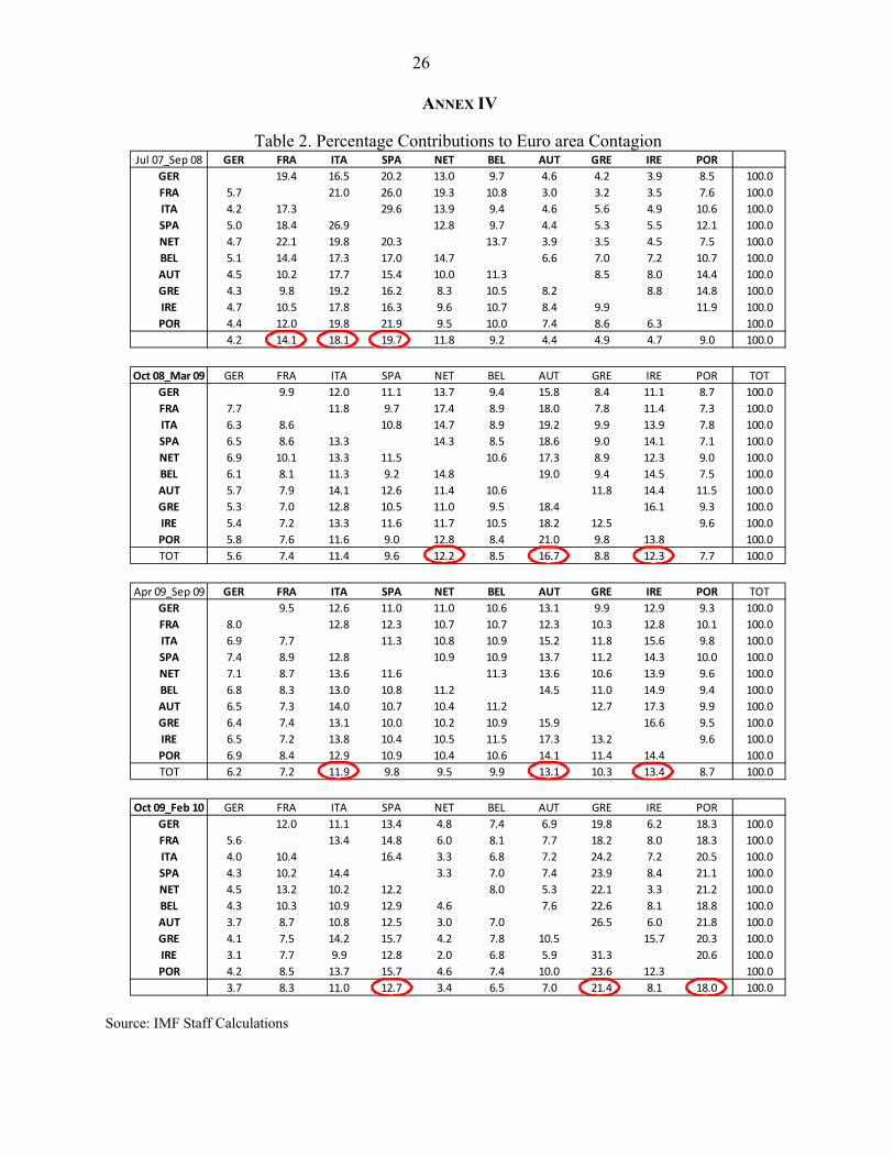
Contagion could be further broken down across sources of distress. In order words, for a given change in the distress dependence of a specific sovereign, we can assess which countries are the most significant sources of contagion during the four phases we previously identified.21 The percentage contributions to the changes in each country’s SC—our measure of distress dependence—can be read along the rows of Table 2 (see Annex IV). 22

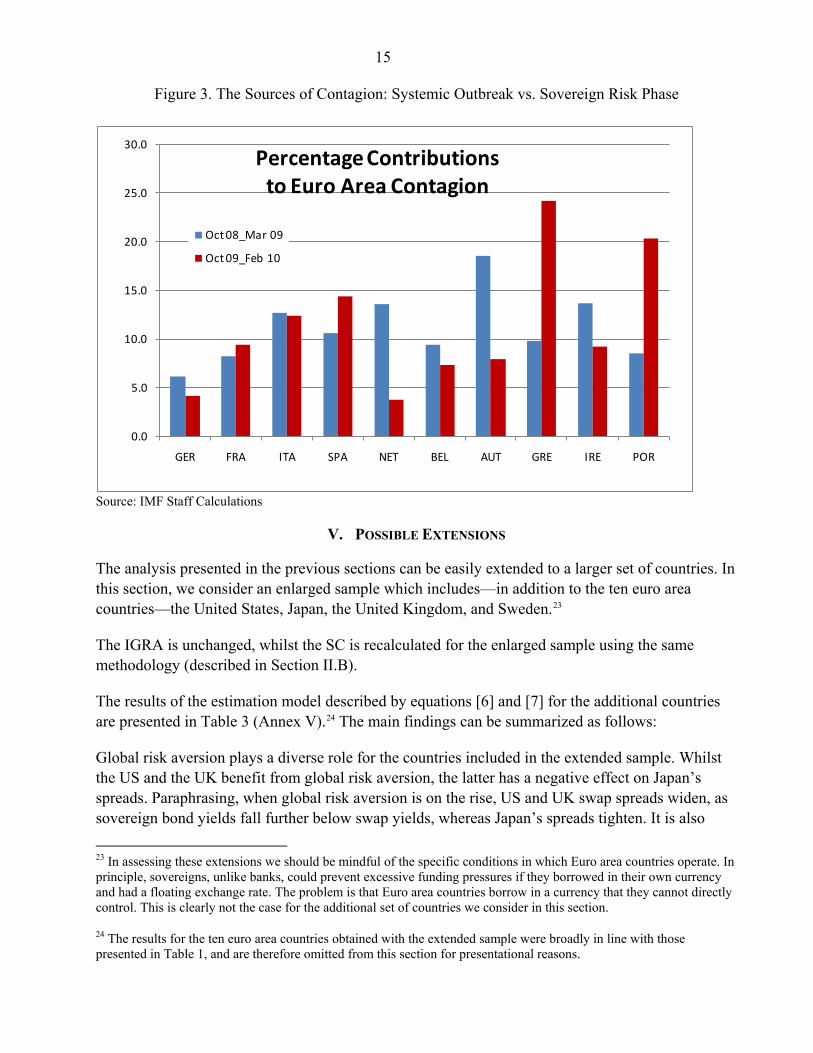
During the systemic response phase, Ireland and Austria remained large perceived sources of contagion together with Italy. Finally, in the sovereign risk phase, the emphasis shifted towards short-term refinancing risk and long-term fiscal sustainability, and the countries putting pressure on the German swap spreads, in other words diluting the credit quality of the Bund became Greece, Portugal, and to some extent Spain and Italy, as highlighted by Figure 3.

During the financial crisis build-up, when contagion did not seem to be a particularly significant factor, the tightening in most swap spreads attributed to contagion stemmed primarily from countries such as Spain, France, and Italy. During the systemic outbreak, however, contagion gained significance and the countries having the largest contribution to the SC were exactly those hit hard by the financial crisis (Austria, the Netherlands, and Ireland), as highlighted by Figure 3.

21 While conditional probabilities do not imply causation, they can provide important insights into interlinkages and the likelihood of contagion.

22 The last row in each table shows the (weighted)-average contribution to the changes in our stress dependence measure (SC) from each of the column countries. This is a proxy for the source of contagion to the other countries in the euro area, emanating from each of these countries during a particular period.

15

Figure 3. The Sources of Contagion: Systemic Outbreak vs. Sovereign Risk Phase

0.0

5.0

10.0

15.0

20.0

25.0

30.0

GER FRA ITA SPA NET BEL AUT GRE IRE POR

Percentage Contributionsto Euro Area Contagion

Oct 08_Mar 09

Oct 09_Feb 10

Source: IMF Staff Calculations

V. POSSIBLE EXTENSIONS

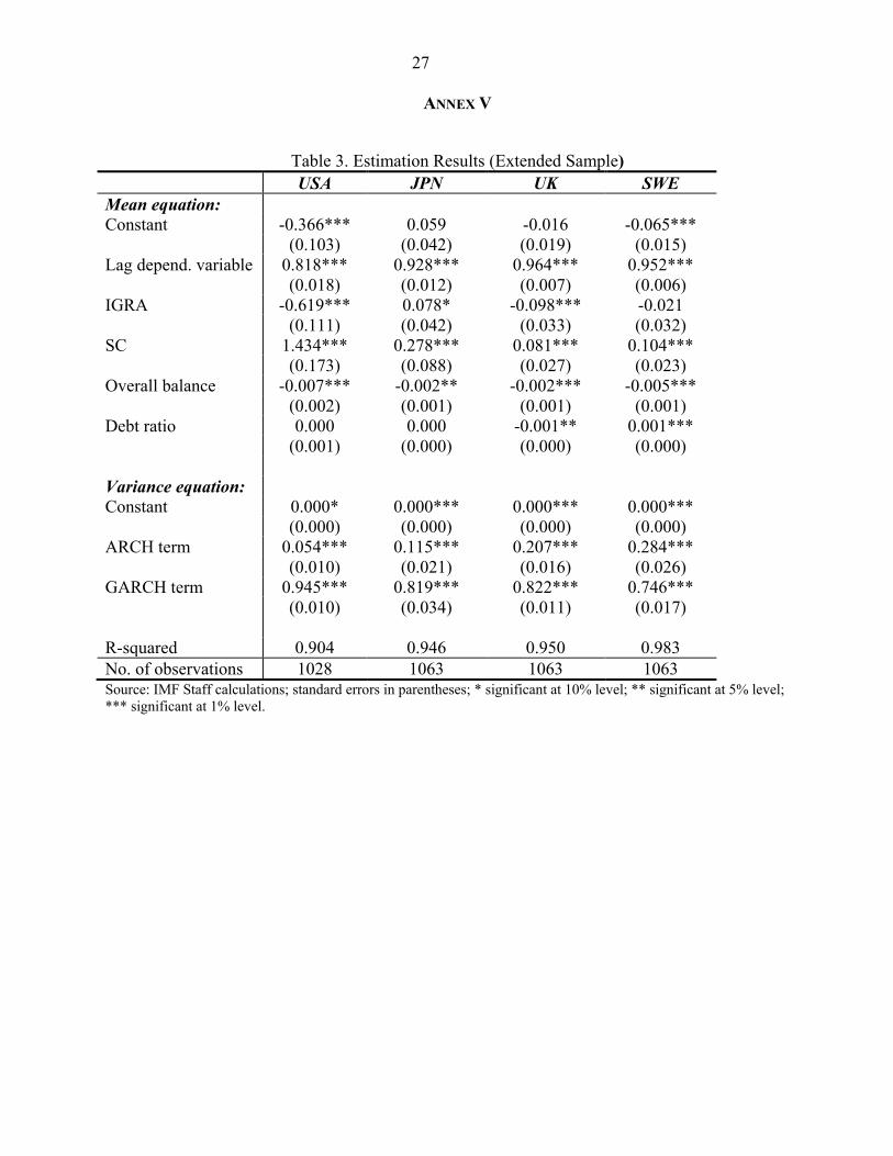
The analysis presented in the previous sections can be easily extended to a larger set of countries. In this section, we consider an enlarged sample which includes—in addition to the ten euro area countries—the United States, Japan, the United Kingdom, and Sweden.23

The IGRA is unchanged, whilst the SC is recalculated for the enlarged sample using the same methodology (described in Section II.B).

The results of the estimation model described by equations [6] and [7] for the additional countries are presented in Table 3 (Annex V).24

Global risk aversion plays a diverse role for the countries included in the extended sample. Whilst the US and the UK benefit from global risk aversion, the latter has a negative effect on Japan’s spreads. Paraphrasing, when global risk aversion is on the rise, US and UK swap spreads widen, as sovereign bond yields fall further below swap yields, whereas Japan’s spreads tighten. It is also

The main findings can be summarized as follows:

23 In assessing these extensions we should be mindful of the specific conditions in which Euro area countries operate. In principle, sovereigns, unlike banks, could prevent excessive funding pressures if they borrowed in their own currency and had a floating exchange rate. The problem is that Euro area countries borrow in a currency that they cannot directly control. This is clearly not the case for the additional set of countries we consider in this section.

24 The results for the ten euro area countries obtained with the extended sample were broadly in line with those presented in Table 1, and are therefore omitted from this section for presentational reasons.

16 worth noting the relative size of this effect in the case of the US. The impact of the IGRA on U.S. swap spreads is far larger than the impact on the spreads for any of the ten euro area countries and the other three countries included in the extended sample. This result emphasizes the notion that U.S. sovereign bonds are perceived as a “safe haven” asset. Finally, in the case of Sweden, risk aversion does not appear to have a statistically significant impact on swap spreads.

Contagion, however, is consistently negative for the government bonds in the four countries included in the extended sample. That is, when the probability of a credit event in a country (given distress in another sovereign issuer) rises, swap spreads tighten, as sovereign bond yields rise closer to the swap yield or move above that level. This is in line with the results obtained for the euro area countries and presented in the previous sections.

Fundamentals also exhibit - in most cases - a significant relationship with these sovereign spreads. Swap spreads tighten, in other words sovereign bond yields rise versus swap yields, when budget deficits increase. In the case of the debt ratios, the latter are not found to have a statistically significant impact on the U.S. and Japan swap spreads. Once again, the perception of the U.S. bonds as a “safe haven” during times of distress seems to make U.S. bond yields relatively inelastic to the supply of government bonds. Similar considerations apply for Japan, as it benefits from strong domestic demand for government bonds by a large pool of high-saving risk-adverse households.

VI. CONCLUSIONS

What factors drove the behavior of swap spreads during the four phases of the crisis outlined in Figure 1? How did contagion among sovereigns evolve during these phases? In order to answer these questions, we estimated a model of swaps spreads based on measures of global risk aversion, contagion, and country-specific fiscal fundamentals.

The paper finds that:

(i) During the phase which we call financial crisis build-up, between July 2007 and September 2008, securities from Germany and, to some extent, other core euro area sovereigns, benefited from flight-to-quality flows, whereas bonds from peripheral countries saw their yields rising versus swap yields as global risk aversion was weighing adversely on these lower-rated issuers. In general, fundamentals were supportive of sovereign bonds, as both the deficit and the debt were still improving at this stage.

(ii) During the systemic outbreak, between October 2008 and March 2009, as sovereigns stepped in and supported financial institutions, government bond yields rose relative to swap yields across the board, on contagion from countries more directly involved in the financial crisis and fundamentals, which had started deteriorating. Global risk aversion was not playing such a favorable role any longer as crisis-related interventions and fiscal stimulus packages had started diluting the perception of sovereigns as a riskless asset class.

(iii) During the systemic response phase, between April 2009 and September 2009, all government bond yields fell back towards swaps, as lower probability of distress in some countries was favorably affecting others. The correction was larger among those bonds such as Italy and Greece

17 which had underperformed during the systemic outbreak as weaker contagion was offsetting further deterioration in fundamentals.

(iv) Finally, in the sovereign risk phase, since October 2009, swap spreads have started to be driven by country-specific developments. They have been broadly unchanged for most countries, but tightening substantially for Greece and Portugal where bond yields have surged well above swap yields on further weakening in fundamentals and intense risk of contagion.

A closer look at distress dependence matrices for each period in the crisis shows that earlier in the crisis the sources of contagion could be found among those countries hit hard by the financial crisis, such as Austria, the Netherlands, and Ireland, whereas more recently the countries putting pressure on Euro area sovereign bonds were primarily Greece, Portugal, and Spain, as the emphasis shifted towards short-term refinancing risk and long-term fiscal sustainability.

The increased emphasis on country-specific risks, directly from worsening fundamentals, or indirectly from spillovers originating in other sovereigns, leads to a number of policy implications. With acute debt vulnerabilities, elevated funding needs, and looming sovereign risk, countries need to invest in their debt management framework and focus on macroeconomic linkages between debt management and financial stability. Debt sustainability and appropriate management of sovereign balance sheets are necessary conditions for preventing sovereign risk from feeding back into broader financial stability concerns. Rising sovereign risk requires credible medium-term fiscal consolidation plans as well as a solid public debt management framework. Emphasis should be given to the presence of significant contingent risk on sovereign balance sheets and the need for sovereigns to gradually disengage from a number of measures supporting the financial sector. More importantly, the crisis has made the link between debt management and financial stability more explicit suggesting the need for closer coordination with monetary and financial stability authorities.

While credible medium-term reforms are implemented and public debt management is improved, immediate steps should be taken to reduce the possibility of projecting longer-term sovereign credit risks into short-term financing concerns. Debt managers across the world have already turned to a broad range of strategies in order to alleviate this intense funding pressure, including adding new instruments to their debt portfolios and making more intense use of syndication techniques as well as raising the size and the frequency of the auctions or revising their format. This effort should be pursued further. Also, authorities should try to remove unnecessary transmission channels of sovereign risk through the financial markets, by being asked to put collateral in swap arrangements.

18

ANNEX I: THE CIMDO-COPULA—INCORPORATION OF CHANGES IN DISTRESS DEPENDENCE AS PROBABILITIES OF DISTRESS (PODS) OF INDIVIDUAL SOVEREIGNS

CHANGE

In order to provide a heuristic explanation of the CIMDO-copula, and how it incorporates changes in distress dependence “automatically” as PoDs of individual sovereigns change, we define a bivariate copula from a parametric distribution and the CIMDO-copula. Segoviano and Goodhart (2009) show that if x and y are two random variables with individual distributions ,x F y H and a joint distribution ( ), .x y G the joint distribution contains three types of information: individual (marginal) information on the variable x, individual (marginal) information on the variable y and information on the dependence between x and y. In order to model the dependence structure between the two random variables, the copula-approach sterilizes the marginal information on x and y from their joint distribution, consequently, isolating the dependence structure. Sterilization of marginal information is done by transforming the distribution of x and y into a uniform distribution, U(0,1), which is uninformative. Under this distribution, the random variables have an equal probability of taking a value between 0 and 1 and a zero probability of taking a value outside [0, 1]. Therefore, this distribution is typically thought of as being uninformative. In order to transform x and y into U (0, 1) the Probability Integral Transformation (PIT) is used. Under the PIT, two new variables are defined as ( ) ( ), ,u F x v H y= = both distributed as U (0, 1) with joint

density [ ],c u v . Under the distribution of transformation of random variables, the copula function

[ ],c u v is defined as:

[ ]( ) ( ) ( ) ( )

( ) ( ) ( ) ( )

1 1

1 1

,, ,

g F u H vc u v

f F u h H v

− −

− −

=

[8]

where g, f, and h are defined densities. From equation [8], we see that copula functions are multivariate distributions, whose marginal distributions are uniform on the interval [0, 1].

Segoviano (2006) shows that the CIMDO distribution with q(x, y) as the prior is of the form:

)

)1 2, ,( , ) ( , ) exp 1 ( ) ( ) .x y

d dx xp x y q x y µ λ χ λ χ

∞ ∞

= − + + + We define 1( ) ( ),c cu F x x F u−= ⇔ = and

1( ) ( ).c cv H y y H v−= ⇔ = Thus, the CIMDO marginal densities take the form,

( ) ( ){ }1 2( ) ( , ) exp 1 ( ) ( ) ,x yd d

c x xf x q x y x y dyµ λ χ λ χ

+∞

−∞ = − + + + ∫ and

( ) ( ){ }1 2( ) ( , ) exp 1 ( ) ( ) .x yd d

c x xh y q x y x y dxµ λ χ λ χ

+∞

−∞ = − + + + ∫

Substituting these into the copula definition we get, the CIMDO-copula, ( , ),cc u v

{ } ( ){ } ( ){ }

1 1

1 12 1

( ), ( ) exp 1( , )

( ), exp , ( ) expy xdd

c c

c

c c xx

q F u H vc u v

q F u y y dy q x H v x dx

µ

λ χ λ χ

− −

+∞ +∞− −

−∞ −∞

− + = − − ∫ ∫

. [9]

19 Equation [9] shows that the CIMDO-copula is a nonlinear function of

1 2, , andµ λ λ , which change as the PoDs of the sovereign under analysis change. Therefore, the CIMDO-copula captures changes in PoDs, as these changes at different periods of the economic cycle.

20

ANNEX II

Table 1. Estimation Results

GER FRA ITA SPA NET Mean equation: Constant -0.247*** -0.162** -0.196** -0.160*** -0.211*** (0.068) (0.073) (0.090) (0.024) (0.028) Lag depend. variable 0.902*** 0.939*** 0.930*** 0.896*** 0.891*** (0.010) (0.009) (0.010) (0.013) (0.013) IGRA -0.251*** -0.327*** 0.005 -0.200*** -0.355*** (0.063) (0.052) (0.063) (0.050) (0.056) SC 0.185** 0.470*** 0.649*** 0.694*** 0.734*** (0.101) (0.070) (0.101) (0.073) (0.081) Overall balance -0.005*** -0.004* -0.005*** -0.003*** -0.006*** (0.001) (0.002) (0.001) (0.001) (0.002) Debt ratio 0.002* 0.000 0.002** 0.001*** 0.001** (0.001) (0.001) (0.001) (0.000) (0.000) Variance equation: Constant 0.000*** 0.000*** 0.000*** 0.000*** 0.000*** (0.000) (0.000) (0.000) (0.000) (0.000) ARCH term 0.227*** 0.256*** 0.119*** 0.321*** 0.220*** (0.024) (0.031) (0.014) (0.036) (0.026) GARCH term 0.784*** 0.751*** 0.882*** 0.691*** 0.780*** (0.020) (0.026) (0.012) (0.026) (0.022) R-squared 0.952 0.956 0.988 0.983 0.967 No. of observations 995 1061 1061 1061 1061 Source: IMF Staff calculations; standard errors in parentheses; * significant at 10% level; ** significant at 5% level; *** significant at 1% level.

21

Table 1. Estimation Results (concluded)

BEL AUT GRE IRE POR Mean equation: Constant -0.068** -0.158*** -0.402*** -0.276*** -0.107*** (0.028) (0.034) (0.057 (0.065) (0.038) Lag depend. variable 0.864*** 0.918*** 0.918*** 0.947*** 0.915*** (0.015) (0.008) (0.007) (0.007) (0.008) IGRA -0.215*** -0.254*** -0.012 -0.203*** -0.319*** (0.052) (0.045) (0.060) (0.055) (0.053) SC 1.188*** 0.933*** 1.662*** 0.988*** 1.453*** (0.116) (0.081) (0.159) (0.100) (0.110) Overall balance -0.006*** -0.003*** -0.001* -0.002*** -0.002** (0.001) (0.001) (0.001) (0.001) (0.001) Debt ratio -0.001 0.000 0.004*** 0.002*** -0.001* (0.000) (0.000) (0.001) (0.001) (0.000) Variance equation: Constant 0.000*** 0.000*** 0.000*** 0.000*** 0.000*** (0.000) (0.000) (0.000) (0.000) (0.000) ARCH term 0.220*** 0.242*** 0.135*** 0.183*** 0.232*** (0.028) (0.028) (0.017) (0.021) (0.029) GARCH term 0.780*** 0.765*** 0.918*** 0.834*** 0.755*** (0.025) (0.024) (0.012) (0.016) (0.023) R-squared 0.978 0.984 0.996 0.997 0.987 No. of observations 995 1061 995 1061 1061 Source: IMF Staff calculations; standard errors in parentheses; * significant at 10% level; ** significant at 5% level; *** significant at 1% level.

22

ANNEX III

Figure 4. Contributions to Changes in Euro Area Swap Spreads

-4.0

-3.0

-2.0

-1.0

0.0

1.0

2.0

3.0

4.0

5.0

2 jul 07 - 30 Sep 08

1 Oct 08 - 31 Mar 09

1 Apr 09 - 30 Sep 09

1 Oct 09 - 2 Feb 10

GermanyFundamentals

Contagion

Global Risk Aversion

23

24

25

Source: IMF Staff Calculations.

26

ANNEX IV

Table 2. Percentage Contributions to Euro area Contagion Jul 07_Sep 08 GER FRA ITA SPA NET BEL AUT GRE IRE POR

GER 19.4 16.5 20.2 13.0 9.7 4.6 4.2 3.9 8.5 100.0FRA 5.7 21.0 26.0 19.3 10.8 3.0 3.2 3.5 7.6 100.0ITA 4.2 17.3 29.6 13.9 9.4 4.6 5.6 4.9 10.6 100.0SPA 5.0 18.4 26.9 12.8 9.7 4.4 5.3 5.5 12.1 100.0NET 4.7 22.1 19.8 20.3 13.7 3.9 3.5 4.5 7.5 100.0BEL 5.1 14.4 17.3 17.0 14.7 6.6 7.0 7.2 10.7 100.0AUT 4.5 10.2 17.7 15.4 10.0 11.3 8.5 8.0 14.4 100.0GRE 4.3 9.8 19.2 16.2 8.3 10.5 8.2 8.8 14.8 100.0IRE 4.7 10.5 17.8 16.3 9.6 10.7 8.4 9.9 11.9 100.0POR 4.4 12.0 19.8 21.9 9.5 10.0 7.4 8.6 6.3 100.0

4.2 14.1 18.1 19.7 11.8 9.2 4.4 4.9 4.7 9.0 100.0

Oct 08_Mar 09 GER FRA ITA SPA NET BEL AUT GRE IRE POR TOTGER 9.9 12.0 11.1 13.7 9.4 15.8 8.4 11.1 8.7 100.0FRA 7.7 11.8 9.7 17.4 8.9 18.0 7.8 11.4 7.3 100.0ITA 6.3 8.6 10.8 14.7 8.9 19.2 9.9 13.9 7.8 100.0SPA 6.5 8.6 13.3 14.3 8.5 18.6 9.0 14.1 7.1 100.0NET 6.9 10.1 13.3 11.5 10.6 17.3 8.9 12.3 9.0 100.0BEL 6.1 8.1 11.3 9.2 14.8 19.0 9.4 14.5 7.5 100.0AUT 5.7 7.9 14.1 12.6 11.4 10.6 11.8 14.4 11.5 100.0GRE 5.3 7.0 12.8 10.5 11.0 9.5 18.4 16.1 9.3 100.0IRE 5.4 7.2 13.3 11.6 11.7 10.5 18.2 12.5 9.6 100.0POR 5.8 7.6 11.6 9.0 12.8 8.4 21.0 9.8 13.8 100.0TOT 5.6 7.4 11.4 9.6 12.2 8.5 16.7 8.8 12.3 7.7 100.0

Apr 09_Sep 09 GER FRA ITA SPA NET BEL AUT GRE IRE POR TOTGER 9.5 12.6 11.0 11.0 10.6 13.1 9.9 12.9 9.3 100.0FRA 8.0 12.8 12.3 10.7 10.7 12.3 10.3 12.8 10.1 100.0ITA 6.9 7.7 11.3 10.8 10.9 15.2 11.8 15.6 9.8 100.0SPA 7.4 8.9 12.8 10.9 10.9 13.7 11.2 14.3 10.0 100.0NET 7.1 8.7 13.6 11.6 11.3 13.6 10.6 13.9 9.6 100.0BEL 6.8 8.3 13.0 10.8 11.2 14.5 11.0 14.9 9.4 100.0AUT 6.5 7.3 14.0 10.7 10.4 11.2 12.7 17.3 9.9 100.0GRE 6.4 7.4 13.1 10.0 10.2 10.9 15.9 16.6 9.5 100.0IRE 6.5 7.2 13.8 10.4 10.5 11.5 17.3 13.2 9.6 100.0POR 6.9 8.4 12.9 10.9 10.4 10.6 14.1 11.4 14.4 100.0TOT 6.2 7.2 11.9 9.8 9.5 9.9 13.1 10.3 13.4 8.7 100.0

Oct 09_Feb 10 GER FRA ITA SPA NET BEL AUT GRE IRE PORGER 12.0 11.1 13.4 4.8 7.4 6.9 19.8 6.2 18.3 100.0FRA 5.6 13.4 14.8 6.0 8.1 7.7 18.2 8.0 18.3 100.0ITA 4.0 10.4 16.4 3.3 6.8 7.2 24.2 7.2 20.5 100.0SPA 4.3 10.2 14.4 3.3 7.0 7.4 23.9 8.4 21.1 100.0NET 4.5 13.2 10.2 12.2 8.0 5.3 22.1 3.3 21.2 100.0BEL 4.3 10.3 10.9 12.9 4.6 7.6 22.6 8.1 18.8 100.0AUT 3.7 8.7 10.8 12.5 3.0 7.0 26.5 6.0 21.8 100.0GRE 4.1 7.5 14.2 15.7 4.2 7.8 10.5 15.7 20.3 100.0IRE 3.1 7.7 9.9 12.8 2.0 6.8 5.9 31.3 20.6 100.0POR 4.2 8.5 13.7 15.7 4.6 7.4 10.0 23.6 12.3 100.0

3.7 8.3 11.0 12.7 3.4 6.5 7.0 21.4 8.1 18.0 100.0

Source: IMF Staff Calculations

27

ANNEX V

Table 3. Estimation Results (Extended Sample)

USA JPN UK SWE Mean equation: Constant -0.366*** 0.059 -0.016 -0.065*** (0.103) (0.042) (0.019) (0.015) Lag depend. variable 0.818*** 0.928*** 0.964*** 0.952*** (0.018) (0.012) (0.007) (0.006) IGRA -0.619*** 0.078* -0.098*** -0.021 (0.111) (0.042) (0.033) (0.032) SC 1.434*** 0.278*** 0.081*** 0.104*** (0.173) (0.088) (0.027) (0.023) Overall balance -0.007*** -0.002** -0.002*** -0.005*** (0.002) (0.001) (0.001) (0.001) Debt ratio 0.000 0.000 -0.001** 0.001*** (0.001) (0.000) (0.000) (0.000) Variance equation: Constant 0.000* 0.000*** 0.000*** 0.000*** (0.000) (0.000) (0.000) (0.000) ARCH term 0.054*** 0.115*** 0.207*** 0.284*** (0.010) (0.021) (0.016) (0.026) GARCH term 0.945*** 0.819*** 0.822*** 0.746*** (0.010) (0.034) (0.011) (0.017) R-squared 0.904 0.946 0.950 0.983 No. of observations 1028 1063 1063 1063 Source: IMF Staff calculations; standard errors in parentheses; * significant at 10% level; ** significant at 5% level; *** significant at 1% level.

28

REFERENCES

Adrian T. and Moench, E. (2008). “Pricing the Term Structure with Linear Regressions”, Federal

Reserve Bank of New York Staff Report No 340. Afonso A. and Strauch, R. (2004). “Fiscal Policy Events and Interest Rate Swap Spreads: Evidence

from the EU”, ECB Working Paper, No.303. Bernoth K., von Hagen, J. and Schuknecht, L. (2004), “Sovereign Risk Premia in the European

Government Bond Market”, ECB Working Paper, No. 369. Black, F. and Scholes, M. (1973). “The Pricing of Options and Corporate Liabilities”, Journal of

Political Economy, 7, 637-654. Cochrane, J. (2001). Asset Pricing, Princeton: NJ, Princeton University Press Codogno, L., Favero, C. and Missale, A. (2003). “Yield spreads on EMU governments bonds”,

Economic Policy, October, 505-32. Coudert, V. and Gex, M. (2008). “Does risk aversion drive financial crises? Testing the predictive

power of empirical indicators”, Journal of Empirical Finance, 15, 67-184. Espinoza, R. and Segoviano, M. (2010). “Probabilities of Default and the Market Price of Risk in a

Distressed Economy”, IMF Working Paper, (forthcoming). Geyer, A., Kossmeier, S., and Pichler, S. (2004). “Measuring systematic risk in EMU government

yield spreads”, Review of Finance, 8, 171-97. Hartelius, K., Kashiwase, K., Kodres, L. (2008) “Emerging Market Spread Compression: Is It Real or Is It Liquidity? ”, IMF Working Paper, 08/10. Kullback, J. (1959). “Information Theory and Statistics”, John Wiley, New York. Luo, L., (2005), Bootstrapping default probability curves, Journal of Credit risk, Volume 1, Number

4, Fall 2005. Manganelli S. and Wolswijk, G. (2007). “Market Discipline, Financial Integration and Fiscal Rules:

What Drives Spreads in the Euro Area Government Bond Market?”, ECB Working Paper, No. 745.

Merton, R. (1974). “On the Pricing of Corporate Debt: The Risk Structure of Interest Rates”,

Journal of Finance, 29, 449-470. Mody A. (2009). “From Bear Stearns to Anglo Irish: How Eurozone Sovereign Spreads Related to

Financial Sector Vulnerability”, IMF Working Paper, 09/108

29 Schuknecht, L., von Hagen, J., and Wolswijk, G. (2010). “Government bond risk premiums in the

EU revisited. The impact of the financial crisis”, ECB Working Paper, No. 1152. Segoviano, M. (2006). “Consistent Information Multivariate Density Optimizing Methodology”.

Financial Markets Group, Discussion Paper No. 557. Segoviano, M. and Goodhart, C. (2009). “Banking Stability Measures”, IMF Working Paper, 09/4. Sgherri, S. and Zoli, E. (2009). “Euro Area Sovereign Risk During the Crisis”, IMF Working Paper,

09/222.