Embed Size (px)
Citation preview
303
[ Journal of Political Economy, 2008, vol. 116, no. 2]� 2008 by The University of Chicago. All rights reserved. 0022-3808/2008/11602-0001$10.00
Sources of Advantageous Selection: Evidencefrom the Medigap Insurance Market
Hanming FangDuke University
Michael P. KeaneUniversity of Technology, Sydney and Arizona State University
Dan SilvermanUniversity of Michigan
We provide evidence of advantageous selection in the Medigap in-surance market and analyze its sources. Conditional on controls forMedigap prices, those with Medigap spend, on average, $4,000 lesson medical care than those without. But if we condition on health,those with Medigap spend $2,000 more. The sources of this advan-tageous selection include income, education, longevity expectations,and financial planning horizons, as well as cognitive ability. Condi-tional on all these factors, those with higher expected medical ex-penditures are more likely to purchase Medigap. Risk preferences do
We thank Pierre-Andre Chiappori, Amy Finkelstein, Alessandro Lizzeri, Jim Poterba,Bernard Salanie, Aloysius Siow, Robert Town, seminar and conference participants atBrown, Concordia, Duke/University of North Carolina, Federal Reserve Bank of New York,Johns Hopkins, Minnesota, Queens, Texas–Austin, Toronto, University of California at LosAngeles, Virginia, Wharton, Wisconsin–Madison, Yale, the National Bureau of EconomicResearch, and the Stanford Institute for Theoretical Economics for helpful suggestions.We especially thank two anonymous referees and the editor, Canice Prendergast, for theirthoughtful comments that significantly improved the paper. Mike Chernew and TamiSwenson assisted us with the access to and clarification of the MCBS data, and John Robstgave us access to Medigap plan pricing data from Weiss Ratings. All remaining errors areour own. Fang and Silverman gratefully acknowledge financial support from the EconomicResearch Initiative on the Uninsured. Keane’s research was supported by Australian Re-search Council grant FF0561843.
304 journal of political economy
not appear as a source of advantageous selection; cognitive ability isparticularly important.
I. Introduction
Asymmetric information is central to modern economic models of in-surance pioneered by Arrow (1963) and Pauly (1974). The classic equi-librium models developed by Rothschild and Stiglitz (1976) and Wilson(1977) assume that potential insurance buyers have one-dimensionalprivate information regarding their risk type. They choose from a menuof contracts, each specifying a premium and amount of coverage, theone best suited to their type. These models predict a positive correlationbetween insurance coverage and ex post realizations of loss. The reasonis ex ante adverse selection: the “bad risks” (i.e., those relatively likelyto suffer a loss) have an incentive to buy more insurance. Allowing forex post moral hazard only strengthens the positive correlation betweencoverage and ex post loss. This “positive correlation property” of classicasymmetric information models forms the basis for empirical tests ofasymmetric information in several recent papers (see Chiappori andSalanie 2000).
These empirical tests, reviewed further in Section II below, generatemixed results. In some markets, such as automobile insurance (e.g.,Chiappori and Salanie 2000) and long-term-care insurance (Finkelsteinand McGarry 2006), there was no statistically significant evidence of thepositive correlation property. Findings like these have fueled an emerg-ing literature on the possibility that multidimensional private infor-mation may lead to what has been called “advantageous selection.” Onthe theoretical side, de Meza and Webb (2001) postulate that individualshave private information about both their risk type and their risk aver-sion.1 They argue that selection based on risk aversion is advantageousif those who are more risk averse both buy more insurance coverageand have lower risks. Failure to condition on risk aversion may thenmask the positive correlation between insurance coverage and ex postrisk predicted by one-dimensional models. Following de Meza andWebb, the existing literature points to risk preferences as the primarysuspect behind advantageous selection. In general, however, any privateinformation could function as a source of advantageous selection if itis positively correlated with insurance coverage and at the same timenegatively correlated with risk.
In this paper, we examine the evidence for and sources of advanta-
1 Hemenway (1990), which used the term “propitious selection,” seems to contain thefirst description of this phenomenon in the economics literature.
sources of advantageous selection 305
geous selection in the “Medigap” insurance market. The Medicare pro-gram provides limited health insurance for U.S. senior citizens. A Medi-gap policy is health insurance sold by a private insurer to fill “gaps” incoverage of the basic Medicare plan (e.g. co-pays, prescription drugs).2
The Medigap market is ideal for studying multidimensional private in-formation and advantageous selection because of two key features.
First, since 1992, the coverage and pricing of Medigap policies havebeen highly regulated by the U.S. government. Specifically, in all butthree states, insurance companies can sell only 10 standardized Medigappolicies; moreover, within the 6-month Medigap open-enrollment pe-riod—which starts when an individual both is older than 65 and isenrolled in Medicare Part B—an insurer cannot deny Medigap coverage,place conditions on a policy, or charge more for pre-existing healthconditions. As shown in the theoretical analysis of Chiappori et al.(2006), in order for multidimensional private information to manifestitself in the form of a violation of the positive correlation property, thesupply side of the insurance market has to be noncompetitive in thesense that the insurance companies are not free to offer any insurancecontract they choose. Thus, the standardization of Medigap policies andthe restrictions on medical underwriting make this market especiallywell suited to studying the evidence for multidimensional privateinformation.
Second, the Medigap market is closely linked to the Medicare pro-gram. As a result, one can obtain detailed administrative data on di-agnoses, treatments, and expenditures of consumers in the Medigapmarket. Specifically, our analysis relies in part on the Medicare CurrentBeneficiary Survey (MCBS), which combines survey data and Medicareadministrative records. The Medicare administrative data on medicalexpenditures provide perhaps the most accurate measure of health ex-penditure risk for a large sample of the entire Medicare population.The MCBS also contains extensive health measures that allow us toobtain accurate measures of ex post expenditure conditional on ageand health. Though the MCBS itself does not contain detailed infor-mation about risk aversion and other potential sources of advantageousselection, the Health and Retirement Study (HRS), a longitudinal dataset covering a large sample of the Medicare-eligible population, hasinformation about such variables. Our empirical strategy uses the MCBSand HRS jointly to examine the sources of advantageous selection.
We find strong evidence of multidimensional private information andadvantageous selection in the Medigap market. Conditional on controlsfor the price of Medigap, we find that medical expenditures for senior
2 See Sec. IV for more details about the Medicare program and the Medigap insurancemarket.
306 journal of political economy
citizens with Medigap coverage are, on average, about $4,000 less thanfor those without. This strong negative correlation between ex post riskand coverage cannot be consistent with “no private information” or“one-dimensional private information” models of the insurance market;thus it directly indicates the presence of multidimensional private in-formation, as well as advantageous selection. Indeed, once we conditionon health (which cannot, by law, be used in Medigap pricing), expen-ditures for seniors with Medigap are about $2,000 more than for thosewithout. These findings indicate that those who purchase Medigap tendto be healthier; that is, there is advantageous selection.
Equally important, we investigate several potential sources of this ad-vantageous selection. This analysis points to variation in cognitive abilityas a prominent source of advantageous selection. We find that elderlycitizens with higher cognitive ability both are more likely to purchaseMedigap and are healthier. We also investigate the potential pathwaysthrough which cognitive ability may act as a source of advantageousselection.
Interestingly, we find that variation in risk preferences, which wasmuch discussed in the previous literature, does not appear to be aprimary source of advantageous selection in the Medigap insurancemarket. Specifically, we find that even though direct measures of risktolerance are significant predictors of Medigap insurance purchase,those who are more risk averse are not particularly healthy; as a result,risk preferences do not much contribute to advantageous selection.3
Our paper is most closely related to Finkelstein and McGarry’s (2006)study of the long-term-care (LTC) insurance market. Using panel datafrom a sample of Americans born before 1923 (the Asset and HealthDynamics among the Oldest Old [AHEAD] study), they find no statis-tically significant correlation between LTC coverage in 1995 and use ofnursing home care in the period between 1995 and 2000, even aftercontrolling for insurers’ assessment of a person’s risk type. This evi-dence, alone, is consistent both with “no asymmetric information” andwith “multidimensional private information.” To distinguish betweenthese stories, they first eliminated the no asymmetric information in-terpretation. Specifically, they found that a subjective probability as-sessment contained in the 1995 AHEAD questionnaire—“What do youthink are the chances that you will move to a nursing home in the nextfive years?”—is positively correlated with both LTC coverage and nursinghome use in 1995–2000, even after controlling for insurers’ risk assess-ment. Since this variable is presumably unobserved by the insurer, these
3 In this regard, our result is similar to that in Cohen and Einav (2007). The authorsinferred both accident risk and risk aversion using an estimated structural model of au-tomobile insurance deductible choice and found that they are positively correlated, con-trary to what is required for risk aversion to be a source of advantageous selection.
sources of advantageous selection 307
positive correlations suggest private information and adverse selectionby the insured.4 Second, they developed a proxy for risk aversion, usinginformation on whether respondents undertake various types of pre-ventive health care. They found that people who are more risk averseby this measure are both more likely to own LTC insurance and lesslikely to enter a nursing home—consistent with multidimensional pri-vate information and advantageous selection based on risk aversion. Infact, their findings suggest that, on net, adverse selection based on riskand advantageous selection based on risk aversion roughly cancel outin the LTC insurance market.
Our paper examines the Medigap market, which, as we argued above,is especially well suited for a study of advantageous selection. In doingso, our paper makes three new contributions to the literature.
First, our method of inference for the presence of multidimensionalprivate information differs from Finkelstein and McGarry’s. We find astatistically significant and quantitatively large negative correlation be-tween ex post medical expenditure and Medigap coverage, controllingfor individual characteristics that are used in pricing. The large negativecorrelation between Medigap coverage and ex post medical expenditureis inconsistent with either no asymmetric information or single-dimen-sional private information, thus leading us directly to an interpretationof the results as evidence of multidimensional private information andat the same time as evidence of advantageous selection.
Second, our paper is, to our knowledge, the first to examine directlymultiple potential sources of advantageous selection. Specifically, in-stead of using behavioral proxies for risk aversion as Finkelstein andMcGarry did, we exploit the direct measures of risk aversion elicitedfrom the respondents in the HRS data. More important, we examinenot just risk preferences as the source of advantageous selection, butalso several other potential sources.
Third, the empirical evidence in our paper suggests that for the Medi-gap insurance market, risk preferences, which were much discussed inthe previous literature, do not appear to be a main source of advan-tageous selection; instead, our results suggest that cognitive ability playsa prominent role. We also explore various channels through which cog-nitive ability may lead to advantageous selection.
The remainder of the paper is structured as follows. Section II reviewsadditional related literature. Section III presents a simple conceptualframework to illustrate the idea of advantageous selection. Section IVprovides some detailed background about Medicare and the Medigap
4 Finkelstein and Poterba (2006) proposed such use of characteristics of insurance buyersthat are observable to the econometrician but not used by insurers in setting prices as ageneral strategy to test for asymmetric information in insurance markets.
308 journal of political economy
insurance market. Section V describes the MCBS and HRS data setsused in our analysis. Section VI provides direct and indirect evidenceof advantageous selection using the MCBS data. Section VII examinesthe sources of advantageous selection by combining the MCBS and HRSand presents our main results. Finally, Section VIII presents conclusions.
II. Related Literature
Within the large literature that tests for the presence of asymmetricinformation, our paper is most closely related to empirical investigationsof the “positive correlation property,” the robust prediction of standardequilibrium models that there should be a positive association betweeninsurance coverage and ex post risk.5 The positive correlation propertyhas been tested in several recent studies of a variety of markets. Theempirical results are mixed and differ by market. For example, in a lifeinsurance market, Cawley and Philipson (1999) found that the mortalityrate of U.S. males who purchase life insurance is below that of theuninsured, even when controlling for many factors such as income thatmay be correlated with life expectancy. In an auto insurance market,Chiappori and Salanie (2000) found that accident rates for youngFrench drivers who choose comprehensive automobile insurance arenot statistically different from the rates of those opting for the legalminimum coverage, after controlling for observable characteristicsknown to automobile insurers. In contrast, Cohen (2005), using datafrom Israel, finds that new auto insurance customers choosing a lowdeductible tend to have more accidents, leading to higher total lossesfor the insurer. Others have examined the evidence of asymmetric in-formation in the choice of insurance contracts such as deductibles, co-payments, and so forth. For example, Puelz and Snow (1994) studiedautomobile collision insurance and argued that, in an adverse selectionequilibrium, individuals with lower risk will choose a contract with ahigher deductible, and contracts with higher deductibles should be as-sociated with lower average prices for coverage. They found evidencein support of each of these predictions using data from an automobileinsurer in Georgia.6 In an annuity insurance market, Finkelstein andPoterba (2004) found systematic relationships between ex post mortalityand annuity characteristics, such as the timing of payments and thepossibility of payments to the annuitant’s estate, but they do not findevidence of substantive mortality differences by annuity size. Yet a third
5 See Chiappori and Salanie (2000). Chiappori et al. (2006) generalize this empiricalprediction to a larger class of models. Chiappori (2001) provides an extensive survey ofthe theoretical and empirical literature.
6 However, see Chiappori and Salanie (2000) and Dionne, Gourieroux, and Vanasse(2001) for critiques of the Puelz and Snow study.
sources of advantageous selection 309
approach is to estimate structural models of health insurance and healthcare choice. For example, Cardon and Hendel (2001) estimated sucha model using data from the National Medical Expenditure Survey. Theyfind that estimated price and income elasticities, as well as demographicdifferences, can explain the expenditure gap between the insured andthe uninsured. Thus they judge the role of adverse selection to beeconomically insignificant.
Our paper is also related to a literature that looks specifically forevidence of adverse selection in the Medigap market. The results fromthat literature are also mixed. For example, Wolfe and Goddeeris (1991),using data from the Retirement History Survey, found that respondentswith better self-reported health were more likely to purchase Medigapand that those with Medigap did not spend more on hospital stays,physician care, and prescription drugs.7 In contrast, Lillard and Ro-gowski (1995), Ettner (1997), and Hurd and McGarry (1997) foundlittle evidence of variation in the probability of purchasing private in-surance by health status. Also related to our paper, Khandker and Mc-Cormack (1999), using MCBS 1991 and 1993, found that those withMedigap tended to incur higher levels of Medicare-reimbursed spend-ing, particularly Part B services. However, because Medigap plans coverMedicare co-pays, they reduce the out-of-pocket price of Medicare-covered services. Thus, it is possible that those with basic Medicare alonemay incur more total expenditures, despite smaller Medicare-reim-bursed expenditures, because they spend more out of pocket. (Indeed,our table 1 in Sec. V.E is consistent with this view.) Thus, we argue that,to study selection in the Medigap market, a better measure of healthexpenditure risk is total medical expenditure, not just expenditure re-imbursed by Medicare or Medigap.8
III. Multidimensional Private Information and AdvantageousSelection
It is now well understood that, given multidimensional private infor-mation, the correlation between ex post risk realizations and coveragemay be negative, zero, or positive (see Hemenway 1990; de Meza andWebb 2001; Jullien, Salanie, and Salanie 2007). These papers all focuson private information about risk aversion as the source of advantageous
7 Khandker and McCormack (1996) estimated multinomial logit models of insurancechoice and found that individuals reporting better health were significantly more likelyto enroll in Medigap plans.
8 Unfortunately, the waves of the MCBS data used in Khandker and McCormack’s (1999)analysis did not contain information about out-of-pocket costs as well as expenses paid bysupplementary insurers. We are grateful to Tami Swenson for the clarification on this dataissue.
310 journal of political economy
selection. In this section, we present a simple conceptual frameworkthat shows how multidimensional private information may lead to ad-vantageous selection.
Consider an individual age 65 or older (and thus covered by Medi-care) who, with probability , will experience a health expen-p � [0, 1]diture shock of size , over and above what is covered by Medicare.9L 1 0For simplicity, assume that the individual can choose to purchase Medi-gap insurance at a premium m that will reduce the out-of-pocket ex-penditure to zero. Let g denote a vector of characteristics that may alsoaffect the individual’s probability of purchasing Medigap. The variablesin g may include risk aversion, but also other characteristics such ascognitive ability, planning horizons, and so forth. Suppose that in thepopulation (p, g) is distributed according to a joint cumulative distri-bution function F. For illustrative purposes, suppose that Q(p, g; L,
is the probability that an individual with risk type p and characteristicsm)g will purchase Medigap when the expenditure shock is L and thepremium is m. For example, if g measures risk aversion, we can showthat is increasing in risk type p and risk aversion g; thatQ(7, 7; L, m)is, more risky and more risk-averse individuals are more likely to pur-chase Medigap (see Fang, Keane, and Silverman 2006). In standardinsurance models in which risk type p is the only dimension of hetero-geneity, g is implicitly assumed to be constant in the population. Forsimplicity, we suppress the dependence of Q on L and m below.
We can describe the “positive correlation property” test of Chiapporiand Salanie (2000) within this simple conceptual framework. The testcompares the average health shock occurrence for those with and with-out Medigap insurance. In our framework, the average health shocksamong those with and without Medigap insurance are respectively givenby
pQ(p, g)dF(p, g)∫ ∫A p (1)Medigap Q(p, g)dF(p, g)∫ ∫
and
p[1 � Q(p, g)]dF(p, g)∫ ∫A p , (2)No_Medigap [1 � Q(p, g)]dF(p, g)∫ ∫
where the denominator in (1) (and respectively in [2]) is the measureof individuals who purchase (respectively, do not purchase) Medigap,and the numerator is the expected number of health shocks that occurto those who purchase (respectively, do not purchase) Medigap. The
9 We assume away the price effect, also called “moral hazard,” by assuming that theexpenditure level L does not depend on health insurance status.
sources of advantageous selection 311
test of the positive correlation property asks whether A 1Medigap
. This condition obviously holds if g is constant in the popu-ANo_Medigap
lation and increases in p. However, if g is heterogeneous in theQ(7, g)population and if at least one element satisfies the following twog � g
conditions,10 then the sign of is ambiguous.A � AMedigap No_Medigap
Property 1. g is positively correlated with insurance coverage; thatis, is increasing in g.Q(p, g)
Property 2. g is negatively correlated with risk p.Moreover, the average probability of insurance purchase for a given
risk type p (after integrating out g), namely, ,Q(p) p Q(p, g)dF (gFp)∫ gFp
may not be monotonic in p if at least one element of g satisfies theabove properties. We will say that private information item g is a sourceof advantageous selection if it satisfies these two properties.
The above discussion is merely illustrative; we only analyze individuals’insurance purchase decisions assuming a particular equilibrium (i.e., aparticular menu of insurance options) and do not consider a morecomplete model in which insurance companies may compete by offeringdifferent insurance contracts. There does not yet exist an equilibriummodel of an insurance market with multidimensional private informa-tion.
In our empirical analysis, we first provide, in Section VI, evidencethat is akin to ; that is, we find that the health ex-A ! AMedigap No_Medigap
penditure risk for those with Medigap insurance is lower than the riskof those without Medigap insurance. This immediately suggests the pres-ence of multidimensional private information generating advantageousselection. Then, in Section VII, we examine the sources of advantageousselection; that is, we look for elements of g that may account for theearlier finding that .A ! AMedigap No_Medigap
IV. Institutional Background
A. Medicare
Medicare is the primary health insurance program for most seniors inthe United States. All Americans age 65 and older who have, or whosespouses have, paid Medicare taxes for more than 40 quarters are eligible.During the period we study, the original Medicare plan consisted ofParts A and B. Part A, the hospital insurance program, covers inpatienthospital, skilled nursing facility, and some home health care. Almost all
10 Of course, any g that is negatively correlated with insurance coverage and positivelycorrelated with risk p will also work. Moreover, the negative correlation between g andrisk p may arise either exogenously or endogenously (in the sense that the would-be insuredwith a higher g may take an action to reduce p). For our purpose this distinction isunimportant.
312 journal of political economy
retirees are automatically enrolled in Part A when they turn 65, andthere are no premiums for this coverage. Medicare Part B, also calledMedicare Insurance, covers Medicare-eligible physician services, out-patient hospital services, certain home health services, and durable med-ical equipment. Part B enrollees have to pay a monthly premium, whichwas $67 in 2004. Almost all people choose to enroll in Part B when theyturn 65. Under Part B, individuals were responsible for a $110 deductiblein 2005 and face a 20 percent co-pay for all Medicare-approved servicesafter exceeding the deductible. The basic Medicare plan is availableeverywhere in the country.11 Some areas also offer what are now calledMedicare Advantage Plans, which are managed care plans (either healthmaintenance organizations [HMOs] or preferred provider organiza-tions). In 2001, approximately 15 percent of Medicare beneficiaries wereenrolled in such Medicare HMOs. We discuss Medicare HMOs furtherin Sections V.C and VI.C. During the period we analyze, Medicare didnot cover prescription drugs.
B. Medigap
While Medicare is the primary health insurance for most older Amer-icans, the program leaves seniors at significant risk of health expendi-tures. On average, basic Medicare benefits cover about 45 percent ofthe personal health care expenditures of aged beneficiaries in theUnited States (Kaiser Family Foundation 2005). To insure Medicarebeneficiaries against some of that risk, private insurance companies sell“Medigap” policies that cover some of the co-pays, deductibles, anduncovered expenses, that is, the “gaps” in the basic Medicare plan.
One reason the Medigap insurance market is ideal for studying mul-tidimensional private information is that, as a result of the OmnibusBudget Reconciliation Act of 1990 (OBRA 1990) effective from 1992,Medigap policies are standardized into 10 plans, A–J, in all states exceptMassachusetts, Minnesota, and Wisconsin.12 The basic plan, A, coversall co-pays for hospital stays longer than 60 days and all co-pays forphysician visits and outpatient care (but not the deductible). All otherplans offer these basic benefits, and more. Details of the different con-stellation of benefits from plans A–J can be found in CMS (2005, 33–35). The restrictions on the Medigap plans have important implicationsfor whether multidimensional private information will manifest itselfthrough a violation of the positive correlation property. Without restric-tions on the insurance contracts that insurance companies can offer,
11 For further details about the coverage offered by Medicare Parts A and B, see CMS(2005, 55–64).
12 These states received waivers that allow them to offer somewhat different standardizedplans.
sources of advantageous selection 313
Chiappori et al. (2006) showed that a suitably modified version of thepositive correlation property still holds even with multidimensional pri-vate information.
OBRA 1990 also regulated Medigap pricing and enrollment in waysthat tend to amplify the asymmetries of information favoring the in-sured. Most important, Medigap policies are required by law to have anopen-enrollment period. This 6-month period begins after the first dayof the first month an individual both is age 65 or older and is enrolledin Medicare Part B. During this period, insurers cannot deny or delayMedigap coverage.13 Moreover, during open enrollment, the federallegislation prohibits insurers from medical underwriting in pricing Med-igap policies; they can effectively price only on age, gender, smokingstatus, and state of residence.14
C. Medigap Pricing
While federal regulations prohibit insurers from medical underwritingin Medigap pricing during the open-enrollment period, in a marketserved by multiple insurers, different firms may price the same policiesdifferently. Indeed, using Medigap premium data from Weiss Ratings,Maestas et al. (2006) documented substantial price variation for thesame Medigap policies. They argued that search costs play an importantrole in explaining the price dispersion for these seemingly homoge-neous products. Robst (2006), using the same data, found that theaverage premium an individual faces for a given Medigap plan dependsalmost exclusively on his or her age, gender, and state of residence.
In our analysis below, we use age, gender, and state of residence tocontrol for Medigap pricing.15 The dispersion in Medigap prices doc-umented by Maestas et al. (2006) does not invalidate these controls forMedigap pricing because, given the federal regulations, during theopen-enrollment period all individuals are offered the same set of Medi-gap plans, and hence they face the same distribution of prices condi-
13 States also have the option of going beyond the federal regulations regarding the 6-month open-enrollment period. Connecticut and New York, e.g., have indefinite openenrollment (i.e., no medical underwriting is ever permitted), whereas California, Maine,and Massachusetts have an annual open-enrollment period of 1 month around a person’sbirthday (Lewin Group 2001).
14 In principle, insurers are free to vary prices by zip code or county. However, the mostcomprehensive Medigap premium data from Weiss Ratings show that, for any given insurer,most premium variation occurs across rather than within states. The reason could be thatthe number of policyholders per zip code or county is too small for risk pooling (seeMaestas, Schroeder, and Goldman 2006).
15 Robst (2006, table 3) showed that less than 10 percent of all available Medigap plansoffered a small average $100 discount for nonsmokers (from Weiss Ratings data). We donot control for smoker status in our basic analysis because such smoker discounts areavailable in only a small number of states.
314 journal of political economy
tional on these variables. It may be that, as Maestas et al. argued, dif-ferences in search costs lead some individuals to face different effectiveprices than others in the same market. If so, it would be important tounderstand the sources of this variation in search costs. Most relevantfor this paper, we would like to know whether cognitive ability and otherfactors function as sources of advantageous selection through their ef-fects on costs of price search. In Section VII.D, we consider in greaterdepth this and other pathways through which cognitive ability and otherfactors induce advantageous selection.
The government also requires that, after the open enrollment, as longas the would-be insured has had Medigap coverage for the past 6 months,enrollment in a different plan offered by the same company be guar-anteed by law. However, if an individual did not enroll in Medigap inthe open-enrollment period or if his or her Medigap coverage lapsed,then insurance companies may subsequently impose both coverage andpricing rules different from those that apply during the open-enrollmentperiod. In these circumstances, our Medigap price controls (age poly-nomial, gender, and state of residence) may not reflect the prices suchindividuals face. Any potential problems caused by such situations, how-ever, are still consistent with our interpretation of advantageous selection(see Sec. VI.D for the details).
V. Data and Descriptive Statistics
Our analysis relies on two large data sets, the MCBS and HRS. Here weprovide a basic description of these data and descriptive statistics of theselected samples in each.
A. Medicare Current Beneficiary Survey
The MCBS began in September 1991 and is a continuous panel surveyof a nationally representative sample of the Medicare population.16 Ben-eficiaries sampled from Medicare enrollment files (or appropriate prox-ies) are interviewed in person, three times a year, using computer-assisted personal interviewing. All the MCBS survey data are linked toMedicare claims and other administrative data. The final file consistsof survey, administrative, and claims data and thus provides a compre-hensive view of respondents’ heath care costs and use.
The central goal of the MCBS is to determine expenditures andsources of payment for all services used by Medicare beneficiaries, in-
16 See http://www.cms.hhs.gov/mcbs/ for more details. A supplemental sample is addedannually in the September–December round to replenish sample cells depleted by refusalsand deaths.
sources of advantageous selection 315
cluding co-payments, deductibles, and uncovered services. This is im-portant, since our focus is on the total health expenditure, that is, thecombined expenditures that were covered by Medicare, other publicinsurance, or private insurance or paid out of pocket. In addition, theMCBS also contains extensive information on the health and demo-graphics of respondents and whether respondents have supplementalinsurance. The Data Appendix (table A1) provides a detailed descriptionof how the variables used in our analysis are constructed.
B. Health and Retirement Study
The HRS began in 1992 as a panel survey of a nationally representativesample of people born between 1931 and 1941 and their spouses. Thisoriginal cohort has been reinterviewed every other year since. In 1998,the objective of the HRS was expanded to include learning about theentire U.S. population over age 50. To achieve this goal, the originalHRS survey was merged with an existing and related survey of individualsborn in 1923 or before, the AHEAD. In addition, two more sampleswere added: the “Children of the Depression” (CODA) cohort bornbetween 1924 and 1930 and the “War Baby” cohort born between 1942and 1947. Our interest in those over age 65 leads us to limit our analysisto health and insurance data collected in the 2000 and 2002 waves ofthe HRS, the latest years for which a final version of the data is available.Whenever possible we include data from all HRS cohorts.17
The HRS is particularly well suited for studying advantageous selectionin Medigap insurance. It contains detailed information about currentand past health status of respondents as well as rich data on their in-surance choices. The health information includes both self-reportedhealth and a very large set of objective measures, such as diseases di-agnosed, and a list of activities the respondent has difficulty performing.The insurance data include information on where the insurance wasacquired, its premiums, and its coverage. The HRS also contains high-quality information about economic and demographic variables. How-ever, the HRS does not have comprehensive information about totalmedical expenditure.18 In Section VII we describe procedures to impute
17 In the end, 37 percent of our combined HRS sample comes from the original HRS,44 percent from AHEAD, and 19 percent from CODA cohort respondents. Because weuse only the 2000 and 2002 waves of the HRS, we use only the 2000 and 2001 waves ofthe MCBS in our main analysis, though we also used lagged health measures from the1999 MCBS in several specification checks.
18 Even with the Medicare claims data that were recently linked to the HRS, we still lackcomprehensive information about medical expenditure that is not paid by Medicare. Astable 1 below shows for the MCBS sample, Medicare-reimbursed expenditure differs sub-stantially from the total medical expenditure.
316 journal of political economy
medical expenditure for the HRS sample using the information in theMCBS.
Equally important, the HRS is unusual in its attention to variablescentral to economic theory, including measures of risk attitudes, lon-gevity expectations, and financial planning horizons; it also containsseveral measures of cognitive ability.19 The measures of risk attitudes weuse are based on HRS respondents’ choices over a series of hypotheticalgambles. The responses to these gambles place respondents into fourordered risk categories. Assuming that an individual’s responses to thesehypothetical income gambles are error-prone reflections of his or herfixed, constant relative risk aversion preferences, Kimball, Sahm, andShapiro (forthcoming) estimate the risk tolerance for each respondentin the HRS by maximum likelihood. In the bulk of our analysis, we usetheir estimates to form our measures of risk aversion (see their table6).20
Longevity expectations may also play a role in determining healthinsurance choices, though the net effect of higher longevity expectationson investment in health is theoretically ambiguous. Those who expectto live longer may want to spend more now on their health since suchinvestment will pay dividends over a longer horizon (see Khwaja 2005).Thus, they would demand more insurance. However, the marginal valueof additional current health investment may be lower when a long lifealready seems likely. The HRS asked of all respondents age 65 andyounger, and repeated in every HRS wave, “What is [percent chance]you will live to 75 or more?” In our analysis, we use the most recentavailable response to this question as our measure of longevityexpectations.21
Similarly, the length of financial planning horizons (which presum-ably reflects both uncertainty and the subjective rate of time discount)may influence insurance choices. Here the effect seems unambiguous,since those with longer horizons would be more willing to pay immediatecosts (premiums) to avoid expected future costs. The HRS collects in-formation on financial planning horizons by asking respondents how
19 Details of these measures can be found in Fang et al. (2006, sec. 5.2).20 While risk attitudes solicited from choices over hypothetical gambles are undoubtedly
measured with error, a number of studies have found the answers to these questions tobe significant predictors of risk-taking behavior. See, e.g., Barsky et al. (1997) on smoking,drinking, and insurance purchase; Lusardi (1998) on wealth accumulation; Charles andHurst (2003) and Kimball et al. (forthcoming) on portfolio choice; Kan (2003) on resi-dential and job mobility; and Schmidt (forthcoming) on the timing of fertility and mar-riage. In Sec. VII.C, we will also find that it is a strong predictor of Medigap purchase.
21 This question presumably measures longevity expectations with error and may reflectboth beliefs about longevity and the degree of certainty about those beliefs. Evidenceconsistent with both error and uncertainty about beliefs is found in the heaping of re-sponses around focal responses such as zero, 50, and, to a lesser extent, 100. See Kezdiand Willis (2005) for a thorough discussion of these measures.
sources of advantageous selection 317
far ahead they plan the family’s saving and spending, ranging from “nextfew months” to “longer than 10 years” in five categories.
Finally, our measure of a person’s cognition combines his or herperformance on four different tests/questions: word recall, a TelephoneInterview for Cognitive Status (TICS) score, subtraction, and numeracy.These scores may proxy for an individual’s degree of economic “ratio-nality,” that is, his or her ability to think through the costs and benefitsof Medigap insurance. Indeed, there is a large body of literature showingthat many of the elderly have difficulty understanding the basic Medi-care entitlement and/or the features of supplemental insurance.22
C. Sample Selection and Medigap Insurance Status
Both the MCBS and HRS contain detailed information about respon-dents’ health insurance choices. Each reports whether the respondentis covered by Medicare, Parts A and B, and whether that coverage isprovided by a Medicare HMO. We also know whether the respondenthad supplemental coverage and, if so, its premium and its source.Given that our goal is to study the decision to buy supplemental insur-ance, our sample should include only people who are covered by basicMedicare (Parts A and B) and do not have access to free (or heavilysubsidized) supplemental coverage provided by a former employer, Med-icaid, or some other government agency (e.g., the Veterans Adminis-tration). That is, we want to limit the sample to people who would haveto pay more than a nominal premium to obtain supplemental coverage.Owing to these considerations, in our analysis we include only respon-dents covered by basic Medicare (including those in a Medicare HMO)and exclude anyone covered by employer-provided health insurance,Medicaid, or other government insurance. In this selected sample, wedefine the Medigap status to be equal to one if the respondent haspurchased additional private insurance that is secondary to Medicare.23
In our main analysis, we treat Medicare HMO enrollees as havingbasic Medicare.24 This choice is motivated by three considerations. First,
22 See, e.g., Harris and Keane (1998) for empirical evidence, Keane (2004) for a surveyof the literature, and Sec. VII.D for additional references.
23 In our working paper (Fang et al. 2006), we also report results from an alternativesample selection in which we retain respondents who have employer-provided supple-mental insurance, provided that they must pay at least $500 per year in premiums for thatinsurance. We then define Medigap status as equal to one if the respondent either haspurchased private insurance that is secondary to Medicare or has employer-provided in-surance for which he or she pays at least $500 in premiums. None of our results, eitherqualitatively or quantitatively, depends on which definition of Medigap status we use.
24 The general view is that Medicare HMOs exchange restrictions on the choices formedical treatment for additional coverage similar to that provided by typical Medigappolicies. Enrollees of Medicare HMOs are discouraged, though not precluded, from pur-chasing additional Medigap insurance policies (see CMS 2005, 5).
318 journal of political economy
60 percent of Medicare HMO enrollees do not pay an additional pre-mium; thus their decision to enroll in a Medicare HMO is often reallya trade-off between restrictions on provider choice and additional cov-erage for the gaps in Medicare; it is not a decision to pay for additionalcoverage. Second, Medicare HMOs are not available in all markets; theyare typically not offered in rural areas. Third, several recent studies haveshown that those who enrolled in Medicare HMOs are, on average,healthier than those on basic Medicare (see Cox and Hogan 1997;Banthin and Taylor 2001). Moreover, Desmond, Rice, and Fox (2006)suggest that greater Medicare HMO enrollment might cause adverseselection into Medigap. Thus, we think that it is conservative to classifyMedicare HMO enrollees as choosing only basic Medicare, in the sensethat it makes it less likely we will find advantageous selection into Medi-gap. However, panel B of table 5 below reports results in which we eithercode Medicare HMO enrollees as having Medigap or instead drop themfrom the analysis. The qualitative results do not change; indeed, asexpected, the evidence for advantageous selection becomes even stron-ger when they are dropped.
D. Measures of Health and Medical Expenditure Risk
Both the MCBS and HRS have detailed and comparable measures ofobservable health indicators including self-reported health, activities ofdaily living (ADL) limitations, instrumental ADL limitations, variousdiagnoses/treatments, and others (see the category Health in the DataAppendix for more details).
For our measure of ex post health expenditure risk, we use “totalmedical expenditure,” which corresponds to the variable pamttot in theMCBS. It is constructed by CMS from a variety of sources, includingMedicare administrative records and survey responses.25 In calculatingpamttot, CMS includes, for any health care event identified either fromthe survey respondent or from the respondent’s Medicare file, paymentsfrom 11 potential sources: Medicare fee-for-service, Medicare HMOs,Medicaid, employer-based private health insurance, individually pur-chased private health insurance, private insurance managed care, privateinsurance from unknown sources, the VA and other public insurance,out-of-pocket payments, and uncollected liability. Thus, the variablepamttot comes as close as possible to measuring total health expenditurefrom all sources.
An important question is whether total medical expenditure is indeedthe most relevant measure of expenditure risk when a would-be insured
25 See MCBS public use documentation on “Cost and Use,” secs. 3 and 5, for moredetails. This documentation is available online at http://www.cms.hhs.gov/apps/mcbs/.

sources of advantageous selection 319
contemplates whether to purchase Medigap. One argument in favor oftreating total medical expenditure as the relevant risk is that Medigappolicies by law cover broad ranges of expenditure not covered by Med-icare (i.e., Medicare deductibles, co-pays, and prescription drugs). Aperson in worse health would typically tend to have greater expenditurerisk in all these areas. Thus, to a good approximation, Medigap planscan reasonably be thought of a simply providing “more” coverage in aunidimensional health risk framework, because by law Medigap planscannot be structured to only cover particular health conditions.
E. Descriptive Statistics
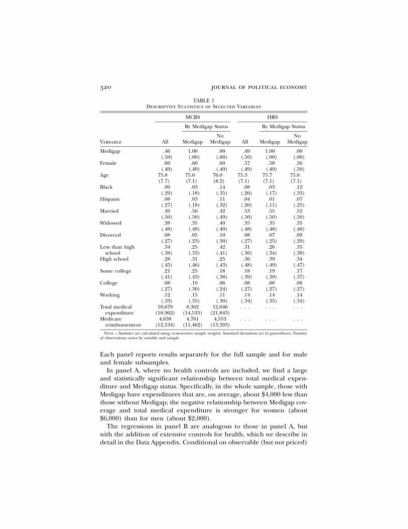
Table 1 provides some descriptive statistics for the Medigap and noMedigap samples, separately for the MCBS and HRS. In both the MCBSand the HRS samples, there are no significant differences between theMedigap and no Medigap subsamples in gender and age, but they dodiffer significantly in their educational attainment and marital status.Interestingly, in the MCBS, the mean total medical expenditure is morethan $12,000 for those with no Medigap, whereas it is only about $8,400for those with Medigap. However, the medical expenditure reimbursedby Medicare is slightly higher for those with Medigap than for thosewithout, consistent with the findings in the literature (see, e.g., Khand-ker and McCormack 1999).
Table 1 also shows that the MCBS and HRS samples are quite similarin the means of the common set of demographic variables. This suggeststhat using the MCBS to impute means and variances of medical expen-diture for the HRS is reasonable.
VI. Evidence of Advantageous Selection
In this section we present a set of simple regressions that together pro-vide strong evidence of advantageous selection in the Medigap market:those who purchase Medigap appear to be healthier and to have lowerex post medical expenditure. We also present direct evidence thathealthier people are more likely to purchase Medigap insurance, con-ditional on observables that determine price.
A. Basic Regression Results: Indirect Evidence of Advantageous Selection
Table 2 reports two panels of results from regressing total medical ex-penditure on Medigap status along with controls for the determinantsof price (gender, a third-order polynomial of age, and controls for stateand year), with or without controlling for health status of the individuals.
320 journal of political economy
TABLE 1Descriptive Statistics of Selected Variables
MCBS HRS
By Medigap Status By Medigap Status
Variable All MedigapNo
Medigap All MedigapNo
Medigap
Medigap .46(.50)
1.00(.00)
.00(.00)
.49(.50)
1.00(.00)
.00(.00)
Female .60(.49)
.60(.49)
.60(.49)
.57(.49)
.58(.49)
.56(.50)
Age 75.8(7.7)
75.6(7.1)
76.0(8.2)
75.3(7.1)
75.7(7.1)
75.0(7.1)
Black .09(.29)
.03(.18)
.14(.35)
.08(.26)
.03(.17)
.12(.33)
Hispanic .08(.27)
.03(.18)
.11(.32)
.04(.20)
.01(.11)
.07(.25)
Married .49(.50)
.56(.50)
.42(.49)
.53(.50)
.55(.50)
.52(.50)
Widowed .38(.48)
.35(.48)
.40(.49)
.35(.48)
.35(.48)
.35(.48)
Divorced .08(.27)
.05(.23)
.10(.30)
.08(.27)
.07(.25)
.09(.29)
Less than highschool
.34(.38)
.25(.33)
.42(.41)
.31(.36)
.26(.34)
.35(.38)
High school .28(.45)
.31(.46)
.25(.43)
.36(.48)
.39(.49)
.34(.47)
Some college .21(.41)
.25(.43)
.18(.38)
.18(.39)
.19(.39)
.17(.37)
College .08(.27)
.10(.30)
.06(.24)
.08(.27)
.08(.27)
.08(.27)
Working .12(.33)
.15(.35)
.11(.30)
.14(.34)
.14(.35)
.14(.34)
Total medicalexpenditure
10,679(18,962)
8,362(14,535)
12,646(21,843)
. . . . . . . . .
Medicarereimbursement
4,638(12,534)
4,761(11,462)
4,553(13,393)
. . . . . . . . .
Note.—Statistics are calculated using cross-section sample weights. Standard deviations are in parentheses. Numberof observations varies by variable and sample.
Each panel reports results separately for the full sample and for maleand female subsamples.
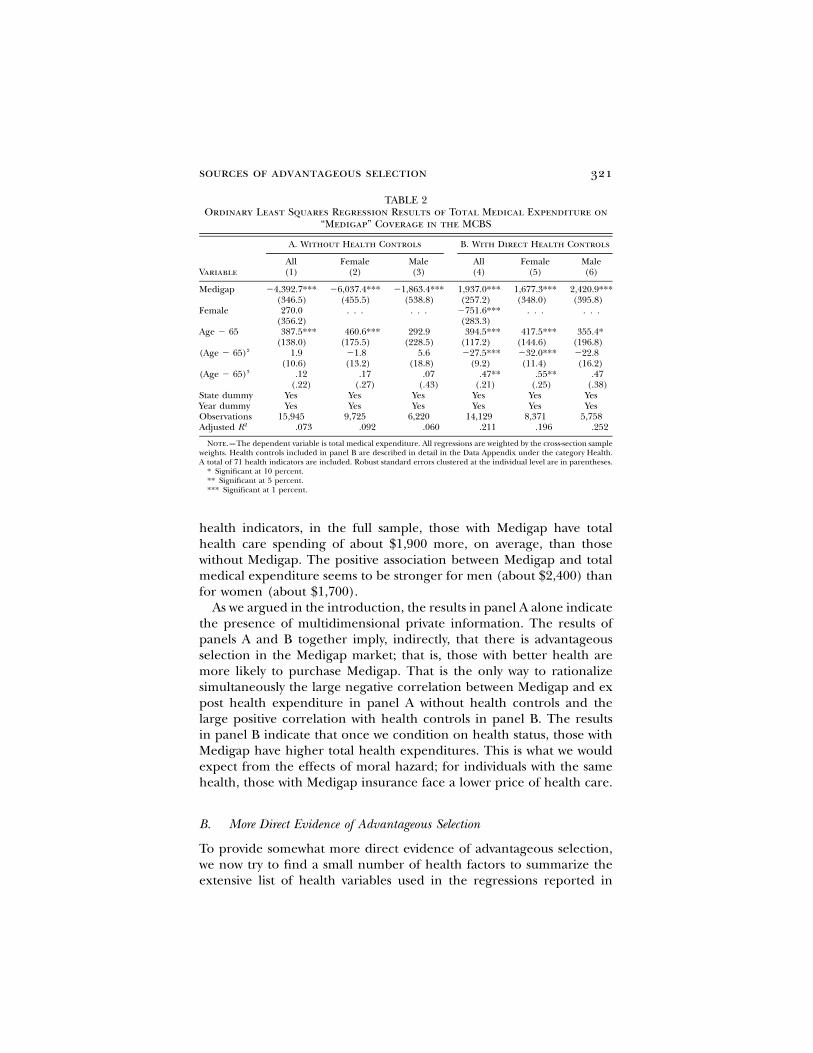
In panel A, where no health controls are included, we find a largeand statistically significant relationship between total medical expen-diture and Medigap status. Specifically, in the whole sample, those withMedigap have expenditures that are, on average, about $4,000 less thanthose without Medigap; the negative relationship between Medigap cov-erage and total medical expenditure is stronger for women (about$6,000) than for men (about $2,000).
The regressions in panel B are analogous to those in panel A, butwith the addition of extensive controls for health, which we describe indetail in the Data Appendix. Conditional on observable (but not priced)
sources of advantageous selection 321
TABLE 2Ordinary Least Squares Regression Results of Total Medical Expenditure on
“Medigap” Coverage in the MCBS
Variable
A. Without Health Controls B. With Direct Health Controls
All(1)
Female(2)
Male(3)
All(4)
Female(5)
Male(6)
Medigap �4,392.7***(346.5)
�6,037.4***(455.5)
�1,863.4***(538.8)
1,937.0***(257.2)
1,677.3***(348.0)
2,420.9***(395.8)
Female 270.0(356.2)
. . . . . . �751.6***(283.3)
. . . . . .
Age � 65 387.5***(138.0)
460.6***(175.5)
292.9(228.5)
394.5***(117.2)
417.5***(144.6)
355.4*(196.8)
(Age � 65)2 1.9(10.6)
�1.8(13.2)
5.6(18.8)
�27.5***(9.2)
�32.0***(11.4)
�22.8(16.2)
(Age � 65)3 .12(.22)
.17(.27)
.07(.43)
.47**(.21)
.55**(.25)
.47(.38)
State dummy Yes Yes Yes Yes Yes YesYear dummy Yes Yes Yes Yes Yes YesObservations 15,945 9,725 6,220 14,129 8,371 5,758Adjusted 2R .073 .092 .060 .211 .196 .252
Note.—The dependent variable is total medical expenditure. All regressions are weighted by the cross-section sampleweights. Health controls included in panel B are described in detail in the Data Appendix under the category Health.A total of 71 health indicators are included. Robust standard errors clustered at the individual level are in parentheses.
* Significant at 10 percent.** Significant at 5 percent.*** Significant at 1 percent.
health indicators, in the full sample, those with Medigap have totalhealth care spending of about $1,900 more, on average, than thosewithout Medigap. The positive association between Medigap and totalmedical expenditure seems to be stronger for men (about $2,400) thanfor women (about $1,700).
As we argued in the introduction, the results in panel A alone indicatethe presence of multidimensional private information. The results ofpanels A and B together imply, indirectly, that there is advantageousselection in the Medigap market; that is, those with better health aremore likely to purchase Medigap. That is the only way to rationalizesimultaneously the large negative correlation between Medigap and expost health expenditure in panel A without health controls and thelarge positive correlation with health controls in panel B. The resultsin panel B indicate that once we condition on health status, those withMedigap have higher total health expenditures. This is what we wouldexpect from the effects of moral hazard; for individuals with the samehealth, those with Medigap insurance face a lower price of health care.
B. More Direct Evidence of Advantageous Selection
To provide somewhat more direct evidence of advantageous selection,we now try to find a small number of health factors to summarize theextensive list of health variables used in the regressions reported in
322 journal of political economy
panel B of table 2 and then directly examine the partial correlations ofthe health factors and Medigap status. We analyzed the extensive list ofhealth variables and found that there are four significant health factorsthat can capture the bulk of variance and covariance in the list of ob-servable health variables. To be conservative, we include five factors forour subsequent analysis. Moreover, by examining the factor loadings(not reported), we can offer interpretations of these factors.26 Factor 1can be interpreted as a “nonresponse” factor, which loads heavily onvariables that are indicators of nonresponse (i.e., there is a nonre-sponder type). Factor 2 loads negatively on self-reported health andpositively on difficulties in instrumental ADLs and thus is an unhealthyfactor. Factor 3 loads positively on self-reported health and negativelyon measured medical conditions in the past 2 years and thus is a healthyfactor. Factor 4 loads positively on self-reported health and self-reportedhealth changes in the last year. It represents a part of self-reported healthnot captured by factors 2 and 3. Factor 5 does not appear to have aclear interpretation.
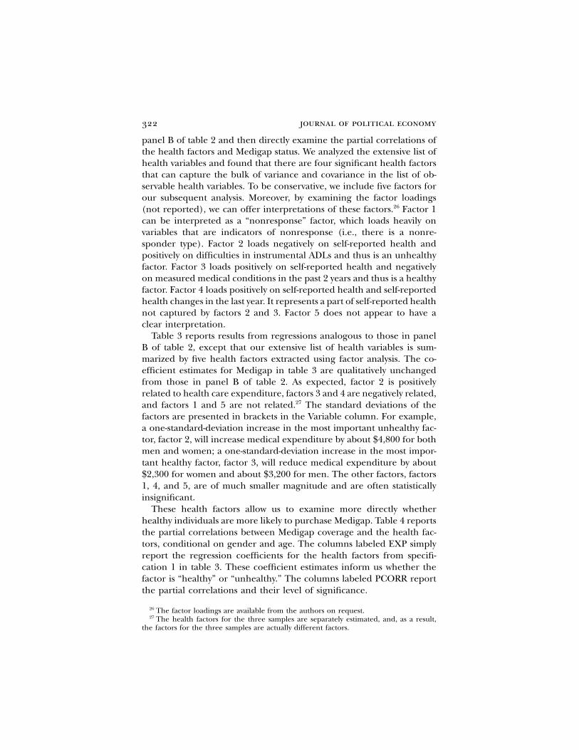
Table 3 reports results from regressions analogous to those in panelB of table 2, except that our extensive list of health variables is sum-marized by five health factors extracted using factor analysis. The co-efficient estimates for Medigap in table 3 are qualitatively unchangedfrom those in panel B of table 2. As expected, factor 2 is positivelyrelated to health care expenditure, factors 3 and 4 are negatively related,and factors 1 and 5 are not related.27 The standard deviations of thefactors are presented in brackets in the Variable column. For example,a one-standard-deviation increase in the most important unhealthy fac-tor, factor 2, will increase medical expenditure by about $4,800 for bothmen and women; a one-standard-deviation increase in the most impor-tant healthy factor, factor 3, will reduce medical expenditure by about$2,300 for women and about $3,200 for men. The other factors, factors1, 4, and 5, are of much smaller magnitude and are often statisticallyinsignificant.
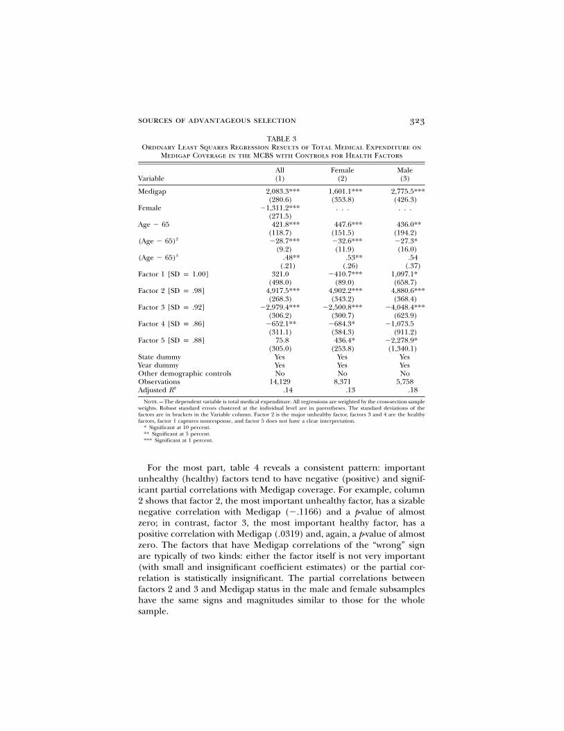
These health factors allow us to examine more directly whetherhealthy individuals are more likely to purchase Medigap. Table 4 reportsthe partial correlations between Medigap coverage and the health fac-tors, conditional on gender and age. The columns labeled EXP simplyreport the regression coefficients for the health factors from specifi-cation 1 in table 3. These coefficient estimates inform us whether thefactor is “healthy” or “unhealthy.” The columns labeled PCORR reportthe partial correlations and their level of significance.
26 The factor loadings are available from the authors on request.27 The health factors for the three samples are separately estimated, and, as a result,
the factors for the three samples are actually different factors.
sources of advantageous selection 323
TABLE 3Ordinary Least Squares Regression Results of Total Medical Expenditure on
Medigap Coverage in the MCBS with Controls for Health Factors
VariableAll(1)
Female(2)
Male(3)
Medigap 2,083.3***(280.6)
1,601.1***(353.8)
2,775.5***(426.3)
Female �1,311.2***(271.5)
. . . . . .
Age � 65 421.8***(118.7)
447.6***(151.5)
436.0**(194.2)
(Age � 65)2 �28.7***(9.2)
�32.6***(11.9)
�27.3*(16.0)
(Age � 65)3 .48**(.21)
.53**(.26)
.54(.37)
Factor 1 [SD p 1.00] 321.0(498.0)
�410.7***(89.0)
1,097.1*(658.7)
Factor 2 [SD p .98] 4,917.5***(268.3)
4,902.2***(343.2)
4,880.6***(368.4)
Factor 3 [SD p .92] �2,979.4***(306.2)
�2,500.8***(300.7)
�4,048.4***(623.9)
Factor 4 [SD p .86] �652.1**(311.1)
�684.3*(384.3)
�1,073.5(911.2)
Factor 5 [SD p .88] 75.8(305.0)
436.4*(253.8)
�2,278.9*(1,340.1)
State dummy Yes Yes YesYear dummy Yes Yes YesOther demographic controls No No NoObservations 14,129 8,371 5,758Adjusted 2R .14 .13 .18
Note.—The dependent variable is total medical expenditure. All regressions are weighted by the cross-section sampleweights. Robust standard errors clustered at the individual level are in parentheses. The standard deviations of thefactors are in brackets in the Variable column. Factor 2 is the major unhealthy factor, factors 3 and 4 are the healthyfactors, factor 1 captures nonresponse, and factor 5 does not have a clear interpretation.
* Significant at 10 percent.** Significant at 5 percent.*** Significant at 1 percent.
For the most part, table 4 reveals a consistent pattern: importantunhealthy (healthy) factors tend to have negative (positive) and signif-icant partial correlations with Medigap coverage. For example, column2 shows that factor 2, the most important unhealthy factor, has a sizablenegative correlation with Medigap (�.1166) and a p-value of almostzero; in contrast, factor 3, the most important healthy factor, has apositive correlation with Medigap (.0319) and, again, a p-value of almostzero. The factors that have Medigap correlations of the “wrong” signare typically of two kinds: either the factor itself is not very important(with small and insignificant coefficient estimates) or the partial cor-relation is statistically insignificant. The partial correlations betweenfactors 2 and 3 and Medigap status in the male and female subsampleshave the same signs and magnitudes similar to those for the wholesample.
324 journal of political economy
TABLE 4Partial Correlation between Medigap Coverage and Health Factors in the
MCBS, Conditional on Gender and Age
Factor
All Female Male
EXP(1)
PCORR(2)
EXP(3)
PCORR(4)
EXP(5)
PCORR(6)
Factor 1 321.0 .03(.00)
�410.7*** .03(.01)
1,097.1* .03(.01)
Factor 2 4,917.5*** �.12(.00)
4,902.2*** �.13(.00)
4,880.6*** �.10(.00)
Factor 3 �2,979.4*** .03(.00)
�2,500.8*** .04(.00)
�4,048.4*** .02(.01)
Factor 4 �652.1** �.02(.04)
�684.3* �.02(.12)
�1,073.5 .02(.08)
Factor 5 75.8 .02(.01)
436.4* .01(.19)
�2,278.9* �.02(.12)
Observations 14,129 8,371 5,758
Note.—The columns labled EXP are the regression coefficients from table 3. They are included in this table for theinterpretation of the factors. The columns labeled PCORR list the partial correlations of Medigap with the correspondingfactors. The numbers in parentheses are the significance levels of the partial correlations.
* Significant at 10 percent.** Significant at 5 percent.*** Significant at 1 percent.
C. Robustness Checks
We now show that our qualitative results about advantageous selectionin the Medigap market are robust to a number of alternative data-codingchoices.
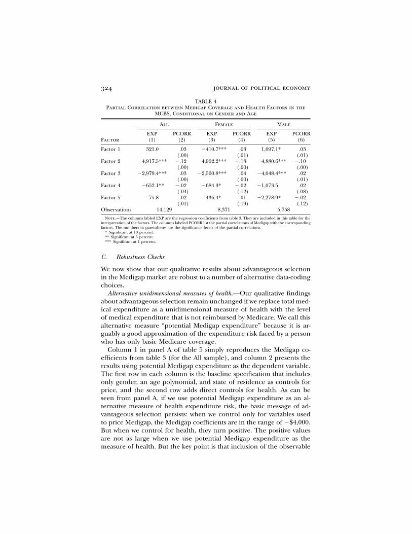
Alternative unidimensional measures of health.—Our qualitative findingsabout advantageous selection remain unchanged if we replace total med-ical expenditure as a unidimensional measure of health with the levelof medical expenditure that is not reimbursed by Medicare. We call thisalternative measure “potential Medigap expenditure” because it is ar-guably a good approximation of the expenditure risk faced by a personwho has only basic Medicare coverage.
Column 1 in panel A of table 5 simply reproduces the Medigap co-efficients from table 3 (for the All sample), and column 2 presents theresults using potential Medigap expenditure as the dependent variable.The first row in each column is the baseline specification that includesonly gender, an age polynomial, and state of residence as controls forprice, and the second row adds direct controls for health. As can beseen from panel A, if we use potential Medigap expenditure as an al-ternative measure of health expenditure risk, the basic message of ad-vantageous selection persists: when we control only for variables usedto price Medigap, the Medigap coefficients are in the range of �$4,000.But when we control for health, they turn positive. The positive valuesare not as large when we use potential Medigap expenditure as themeasure of health. But the key point is that inclusion of the observable
sources of advantageous selection 325
TABLE 5Robustness of the Evidence of Advantageous Selection: Medigap Coefficients
A. Alternative Measures of Health Expenditure Risk
HealthControls
TotalMedical
Expenditure(1)
PotentialMedigap
Expenditure(2)
No �4,392.7***(347.0)
�4,454.0***(202.2)
Yes 1,937.0***(257.6)
80.4(132.1)
B. Alternative Treatment of Medicare HMO
HealthControls
Treated asMedigap
(1)
Droppedfrom Sample
(2)
No �4,418.5***(364.8)
�3,996.8***(298.7)
Yes 1,899.6***(276.6)
2,011.3***(276.6)
C. Trimming Top 5 Percent of the Observations
HealthControls
TotalMedical
Expenditure(1)
PotentialMedigap
Expenditure(2)
No �1,400.1***(183.1)
�1,103.3***(94.4)
Yes 1,673.2***(147.8)
247.7***(73.8)
D. Including Additional Demographic Controls
HealthControls
All(1)
Female(2)
Male(3)
No �3,783.3***(375.4)
�5,687.4***(485.7)
�1,448.2***(569.8)
Yes 1,732.8***(272.4)
1,426.2***(358.4)
2,210.1***(418.9)
Note.—All regressions are weighted by the cross-section sample weights. The descriptions of the direct healthcontrols can be found in the Data Appendix. The additional demographic controls used in panel D include race,education, marital status, income, working, and number of children. Robust standard errors in parentheses areclustered at the individual level.
* Significant at 10 percent.** Significant at 5 percent.*** Significant at 1 percent.
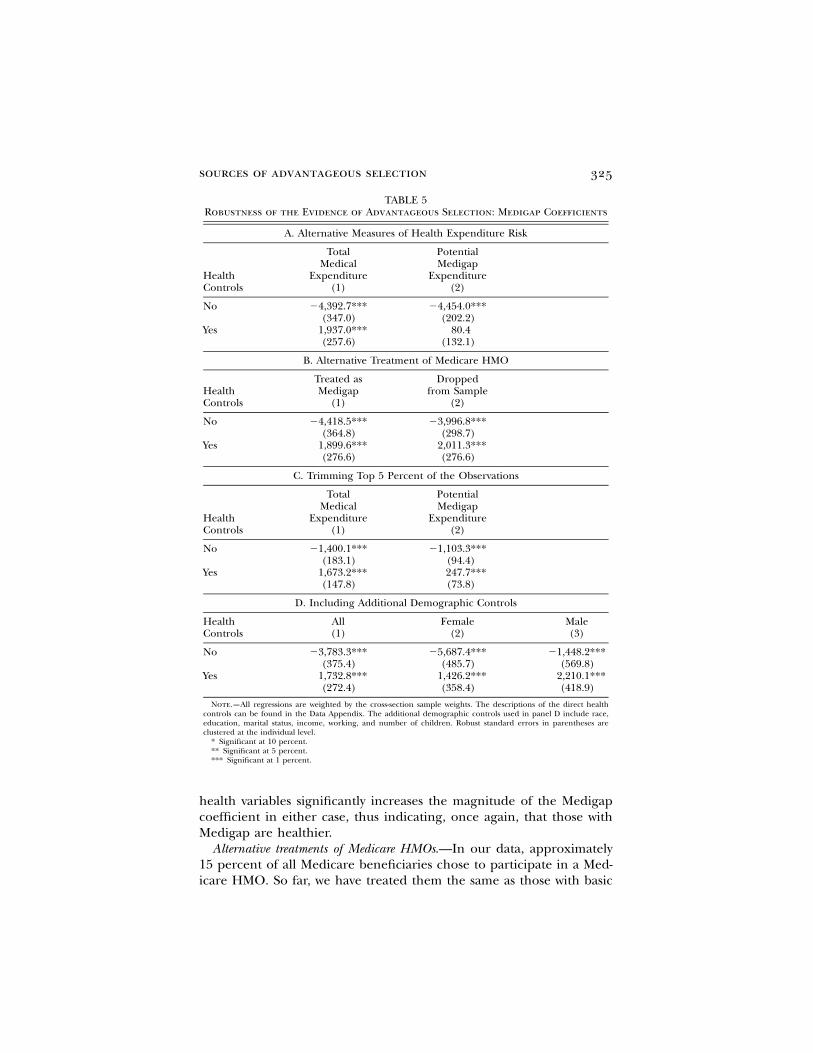
health variables significantly increases the magnitude of the Medigapcoefficient in either case, thus indicating, once again, that those withMedigap are healthier.
Alternative treatments of Medicare HMOs.—In our data, approximately15 percent of all Medicare beneficiaries chose to participate in a Med-icare HMO. So far, we have treated them the same as those with basic
326 journal of political economy
fee-for-service Medicare. We now show the results with two alternativetreatments of those with Medicare HMOs: we either code them as havingMedigap or code them as missing (thus dropping them from ouranalysis).
Panel B of table 5 reports the Medigap coefficient estimates underthe two alternative treatments of Medicare HMOs. Column 1 shows thatthe recoding of Medicare HMO participants as Medigap actually some-what strengthens the findings of advantageous selection reported earlier.For example, the negative Medigap coefficient becomes somewhat morenegative. This is not surprising given the consensus in the literature(noted earlier) that there is advantageous selection into MedicareHMOs. Similarly, dropping those observations from our analysis doesnot change the results, either qualitatively or quantitatively.
Trimming the outliers.—It is well known that the distribution of medicalexpenditure is right skewed. For example, in our selected sample, totalmedical expenditure has a skewness of 4.2, with a mean of $10,679 anda median of $3,467; potential Medigap expenditure has a skewness of3.5, a mean of $6,040, and a median of $2,292. In our view, outliermedical expenditures are likely an important concern when individualsconsider whether to purchase Medigap. Nevertheless, we show in panelC of table 5 that the findings of advantageous selection are not solelydriven by the highest expenditure levels. In column 1 we report theMedigap coefficient estimates after we drop the observations whose totalmedical expenditure is above the ninety-fifth percentile. The coefficientestimates, not surprisingly, get smaller in absolute magnitude, but thequalitative conclusion regarding the presence of advantageous selectionis not affected. Column 2 reports the results for potential Medigapexpenditure after we trim the top 5 percent. Again, the coefficients aresmaller in magnitude, but the qualitative results are the same.
D. Discussion
In this subsection we consider a few issues of potential concern regard-ing the interpretation of our findings.
Insurers’ selection.—A natural question is whether the advantageousselection we documented for the Medigap insurance market is, as weinterpret it, driven by consumers or is instead induced by insurers.Insurers have incentives to “cream-skim,” that is, target their offeringsat relatively good risks, because medical underwriting is prohibited.Three observations cast some doubt on the importance of cream-skim-ming in explaining the advantageous selection we observe. First, thebest evidence for cream-skimming in related markets comes from se-lection into Medicare HMOs, not Medigap, and in our main analysiswe classify those in Medicare HMOs as in basic Medicare. And as we
sources of advantageous selection 327
saw in Section VI.C, dropping Medicare HMO enrollees from the anal-ysis has little effect on our estimates of advantageous selection intoMedigap. (Indeed, if anything, the evidence for advantageous selectionbecomes stronger, consistent with cream-skimming in the MedicareHMOs.)
Second, as Maestas et al. (2006) noted from the data from WeissRatings, about two-thirds of the Medigap policies sold are agent-solicitedand only about one-third are sold by the insurance companies directly.It seems likely that the incentives of agents and insurance companiesare not perfectly aligned: agents want to sell policies and care less aboutthe risk to the insurance company of a given contract. Thus, withoutcompensation schemes that reflect ex post risk, agents will choose tolocate their offices and market their products where they can sell in-surance and pay little attention to ex post risks to the insurancecompanies.
Third, we can ask whether the extent of advantageous selection ismitigated if we condition on observable demographics of the consumers,including race, education, marital status, income, working status, andnumber of children, which insurance companies could use to cream-skim to the extent that they may be correlated with the health expen-diture risks of the insured.28 Panel D of table 5 reports the Medigapcoefficients with and without health controls, but including the abovelist of additional demographic controls. Controlling for the additionaldemographics does lower the magnitude of the Medigap coefficient,but only modestly. For example, without health controls, expendituresfor those with Medigap are about $3,800 less than for those withoutMedigap for the whole sample, compared to $4,400 without the de-mographic controls. Similarly, with direct health controls, the Medigapcoefficient estimate falls only slightly to $1,700 with the additional de-mographic controls for the whole sample, compared to $1,967 without.The effects of these additional demographic controls are similar in thefemale and male samples. This evidence suggests that our finding ofadvantageous selection is not mainly driven by insurers’ selection.
Panel D of table 5 can also be seen to show that even though theseadditional demographic variables can explain part of the observed ad-vantageous selection, the extent is rather limited. As a result, in thenext section we will extend our search for the sources of advantageousselection.
Endogenous health measures.—Another possible concern is that thehealth measures we used in our analysis could be affected by Medigap
28 It is important to emphasize that, in order to establish the existence of advantageousselection, we should not include these additional demographic variables because insurancecompanies are not allowed to price on them.
328 journal of political economy
insurance status itself. It is possible that if those with Medigap are morelikely to seek care, they may be more likely to have certain conditionsdiagnosed. This would make the Medigap population seem less healthythan they actually are (relative to the basic Medicare population). Thiswould cause them to have lower than expected expenditure (conditionalon health), thus biasing the Medigap coefficient in panel B of table 2in a negative direction (i.e., we would understate the degree of advan-tageous selection).29
Selection in Medigap renewal.—Yet another potential concern is that ourMedigap price controls (age polynomial, gender, and state of residence)do not reflect the prices faced by those who let their coverage lapsebecause the prohibition on medical underwriting in Medigap pricingapplies in most states only in the open-enrollment period. In this case,our finding that expenditures for those with Medigap are about $4,000less than for those without may, to some extent, reflect the followingpossibility: those without Medigap are less healthy because their cov-erage previously lapsed and, moreover, they are currently priced out ofMedigap because of their poor health. Because the MCBS panel is rel-atively short, we do not have Medigap coverage information for a largenumber of individuals since their open enrollment. However, we arguehere that if the mechanism described above is influencing our estimates,its effect is nonetheless consistent with our interpretation of advanta-geous selection.
Consider the group of individuals without Medigap who are unhealthyand are priced out of Medigap because of a lapse in their coverage.One possibility is that they never purchased a Medigap policy in thefirst place. This would be consistent with our interpretation of advan-tageous selection: less healthy individuals are less likely to purchaseMedigap during open enrollment (when everyone is approximately thesame age, and thus state and gender controls alone would be sufficientto control for Medigap pricing). The second possibility is that thosecurrently without Medigap did purchase a policy during open enroll-ment but subsequently failed to renew. The standard adverse selectionmodel with one-dimensional private information about risk would havesuggested that less healthy people should be more likely to renew, justas they should be more likely to enroll in the first place. If, in contrast,less healthy people are less likely to renew, this is again a form of ad-vantageous selection, albeit in the renewal stage.
29 In any case, our results are not changed if we perform our analysis using lagged,instead of current, health indicators.
sources of advantageous selection 329
VII. Sources of Advantageous Selection
In this section we investigate the sources of advantageous selection. Thatis, we seek to identify dimensions of individuals’ private informationthat satisfy the two properties we mentioned in Section III, that is, un-priced variables that both (i) make individuals more likely to purchaseMedigap and (ii) are negatively correlated with their health expenditurerisk.
A. Empirical Strategy
The ideal data set for our analysis would be the HRS augmented bylinks to Medicare administrative data containing information on totalmedical expenditure. Unfortunately, the HRS is not yet properly linkedto the Medicare administrative records and has imperfect informationon out-of-pocket spending or spending reimbursed by other sourcesrelative to MCBS. On the other hand, the MCBS does not contain in-formation about many suspected sources of advantageous selection. Wenow describe our empirical strategy, which combines the MCBS and theHRS to examine the sources of advantageous selection.30
The data in the MCBS can be written as
{E , M , H , D } (3)i i i i i�IMCBS
and the data in the HRS as
{M , H , D , X } , (4)j j j j j�IHRS
where and denote the MCBS and HRS samples, respectively.I IMCBS HRS
Note that the variables , which denote Medigap coverage,{M, H, D}health measures, and demographics, are common to both data sets. ButE, total medical expenditure, appears only in the MCBS, and X, the listof variables that we think are potential sources of advantageous selec-tion, appears only in the HRS.
Our strategy is simple and consists of two steps. In the first step, weuse the MCBS data to estimate prediction equations for total medicalexpenditure risk as well as its variance. (We describe our imputationstrategies in the next subsection.) These equations will use only covar-iates that are also available in the HRS, so we can use the estimatedprediction equations from the MCBS data to impute the mean ( ) andEj
variance ( ) of health expenditures for each person in our HRSVarj
30 There is a sizable literature on empirical methods to deal with the incomplete databy combining multiple data sets. For an excellent survey, see Ridder and Moffitt (2007).
330 journal of political economy
sample. With the imputed and , our augmented HRS data canˆ E Varj j
now be represented as
ˆ {M , H , D , X , E , Var } . (5)j j j j j j j�IHRS
In the second step, we first regress Medigap coverage on expected ex-penditure and pricing variables:
ˆM p d � d E � d D � � , (6)j 0 1 j 2 j j
where, as before, the variables in include a third-order polynomialDj
in age, gender, and state of residence to capture the pricing of Medigapinsurance. As we report below, and consistent with our finding in SectionVI, we obtain a negative and significant estimate for d1, the coefficienton expected expenditure, implying advantageous selection in the pur-chase of Medigap in the HRS. We then gradually add potential sourcesof advantageous selection from the list of variables contained in {X ,j
. We will show below that when we estimate the partial correlationVar }jbetween Medigap coverage and health expenditure risk, controlling notonly for the determinants of price, , but also for , the partialD {X , Var }j j j
correlation will turn positive. More precisely, when we estimate
ˆ M p v � v E � v risktol � v Var # risktol � v Varj 0 1 j 2 j 3 j j 4 j
� v X � v D � � , (7)5 j 6 j j
we find that is positive and significant—consistent with the positivev1
correlation property predicted by standard insurance models with unidi-mensional private information. This is the sense in which we say wehave successfully identified several key sources of advantageousselection.
B. Imputation Strategies
Our empirical strategy requires a determination about which sample ofthe MCBS to use in estimating the prediction equations. Conceptually,we want a measure of expenditure risk for a person who has basicMedicare and is considering whether to buy Medigap. To obtain sucha measure, it is not clear whether we should estimate prediction equa-tions using only data for those without Medigap or whether we shouldinstead include the whole MCBS sample. We follow a practical strategyand estimate the prediction equations both ways. We explain below thatbiases induced by each method may be slight and are likely to understatethe extent of advantageous selection. Later we show that our results arerobust to which method we use.
Imputation using the MCBS subsample with no Medigap coverage.—With

sources of advantageous selection 331
the first method, we use only the subsample in the MCBS with noMedigap coverage to estimate the mean and variance of medical ex-penditures. Suppose that the mean and variance prediction equationsobtained from the MCBS are
ˆ ˆ ˆ ˆE p a � a H � a D (8)i1 0 1 i 2 i
and
2 ˆ ˆ ˆˆVar p (E � E ) p b � b H � b D . (9)i1 i i1 0 1 i 2 i
We can then impute the mean and variance of medical expendituresfor the HRS sample as follows: for each , the imputed meanj � IHRS
medical expenditure is
ˆ ˆ ˆ ˆE p a � a H � a D , (10)j1 0 1 j 2 j
and the imputed variance of medical expenditure is
ˆ ˆ ˆVar p b � b H � b D . (11)j1 0 1 j 2 j
Imputation using the whole MCBS.—With the second method, we usethe whole MCBS sample. In this case, we include in the regressions aMedigap status indicator . That is,Mi
ˆ ˆ ˆ ˆ ˆE p h � h M � h H � h D (12)i2 0 1 i 2 i 3 i
and
2 ˆ ˆ ˆ ˆˆVar p (E � E ) p y � y M � y H � y D . (13)i2 i i2 0 1 i 2 i 3 i
We then impute the mean and variance for each member ofj � IHRS
the HRS sample as follows:
ˆ ˆ ˆ ˆE p h � h H � h D (14)j2 0 2 j 3 j
and
ˆ ˆ ˆVar p y � y H � y D . (15)j2 0 2 j 3 j
Note that in the imputation equations (14) and (15), we set equalMj
to zero for the HRS sample. Thus the predictions above pertain to themean and variance of medical expenditures for a person without Medi-gap coverage.
Discussion of the imputation methods.—If, conditional on and , se-H Dj j
lection into Medigap were random, then either of the two approachesoutlined above would be conceptually correct. The list of observablehealth variables that we include in our imputation is extremely detailed,
332 journal of political economy
so it may be that selection based on unobserved health is not quanti-tatively important.31
If, however, there is nonrandom selection into Medigap conditionalon and , each imputation method will have limitations. ConsiderH Dj j
the first method. If those with Medigap have systematically better un-observed health (just as they have better observed health), then willEj1
tend to overestimate the expected medical expenditure for those inHRS who actually have Medigap. This bias will cause us to understatethe degree of advantageous selection in the HRS. Using the secondimputation method, we need to include the Medigap status indicator
in prediction equations (12) and (13). Otherwise we will exaggerateMi
the pre-Medigap purchase expenditure risk by including the “moralhazard” or price effect of Medigap coverage. However, given the selec-tion into Medigap, the Medigap coefficient will be biased. For example,if those with Medigap have systematically better unobserved health(just as they have better observed health), the Medigap coefficient willbe downward biased (i.e., we understate the price effect). This wouldcause to, again, overstate the pre-Medigap expenditure risk for thoseEj2
who actually have Medigap.
C. Sources of Advantageous Selection: Main Findings
This subsection reports our main results regarding the sources of ad-vantageous selection. Panels A and B in table 6 report, respectively,results based on the two methods of imputing health expenditure riskdescribed above. In each panel, columns 1–3 report estimates of thecoefficient on predicted health expenditure (with the correspondingEj
p-values of the estimates in parentheses) in equations (6) and (7) forsamples of varying sizes.32 (The sample sizes change because of theadditional variables that we explain below.) We enter into the re-Ej
gressions in tens of thousands of dollars ($10,000) to make the resultseasier to interpret. Columns 4–11 indicate the list of control variablesincluded in X, with Y (N) indicating that a particular variable is (is not)included. Column 12 gives the sample size for the regression.
Here we explain the decline in the number of observations due to
31 The (unadjusted) is around .3 in the regressions for E and around .2 in the2Rregressions for Var. The relatively low ’s are not surprising because medical expenditures2Rare intrinsically highly random. Thus, low ’s do not mean that the model does a poor2Rjob of predicting expected medical expenditures for a certain type of person. It shouldalso be noted that this does not reveal whether the random selection assumption is rightor wrong.
32 We adjusted the standard errors for the coefficient estimates of to account forEj
the fact that was estimated in the first step. Specifically, we calculated the varianceEj
of the first-step prediction errors, which is then multiplied by and added to the2v1
estimated variance of the second-step regression residuals.
sources of advantageous selection 333
missing values as we add more variables to the regressions.33 Two vari-ables lead to substantial loss of observations: First, adding risk toleranceto the regression eliminates about two-thirds of the sample because theHRS asked these questions of only about one-third of the subsample.Second, when we include the cognition variables (in particular, cogni-tion questions related to numeracy), we lose another half of the sample.In order to avoid the possibility that our results are driven by the chang-ing samples, we rerun all our regressions on three samples. Column 1reports results using the full sample, column 2 for the medium sample(for which the risk tolerance measure is available), and column 3 forthe smallest sample (for which the cognition variables are also available).
Now we explain the key findings from table 6.• Rows 1 and 9 show that, regardless of the imputation method, if we
do not control for any of the variables, individuals with higher healthX j
expenditure risk (measured by ) are less likely to purchase Medigap.Ej
For the sample with the most complete data, the point estimates implythat a $10,000 increase in health expenditure risk reduces the proba-bility of buying Medigap by 4.6–5.7 percentage points. This, of course,is simply a confirmation (from a different angle and using differentdata) of our finding of advantageous selection reported in Section VI.
• Rows 2 and 10 add risk tolerance alone to the regression (6). Thisspecification is important because the previous literature we have cited,both theoretical and empirical, has focused almost exclusively on riskaversion as the source of advantageous selection. When rows 2 and 10,respectively, are compared with rows 1 and 9, the inclusion of risk tol-erance only slightly reduces, if at all, the magnitude of the negativecoefficient on predicted health expenditures.34 However, risk tolerance,as predicted by standard economic models, is a significant predictor ofMedigap purchase: when it is entered as a set of dummy variables, anF-test rejects the null hypothesis of joint insignificance with a p-value ofless than .001; indeed more risk-tolerant individuals are less likely topurchase Medigap. Importantly, more risk-tolerant individuals are notespecially unhealthy. Thus, in the language we used in Section III, whatwe find here is that risk aversion (the opposite of risk tolerance) satisfiesproperty 1 but does not satisfy property 2, which is also necessary forit to be a source of advantageous selection in the Medigap insurancemarket.
• Results change, however, when we also control for the variance of
33 Most of the missing values result from the relevant survey questions not being askedinstead of nonresponse.
34 This result does not depend on the linear specification for the effect of risk tolerance.If, instead, risk tolerance enters as a third-order polynomial or as a complete set of dummyvariables, the point estimate of the coefficient on is essentially unchanged from thatEj
without the inclusion of risk tolerance.
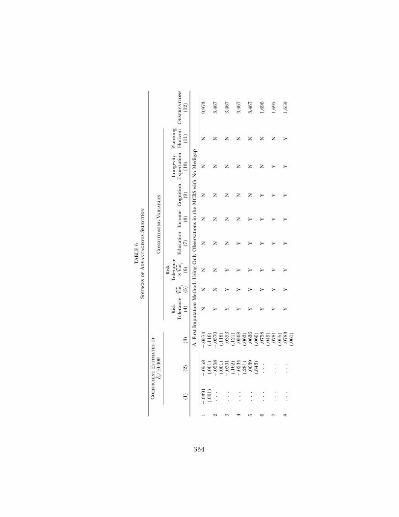
334
TA
BL
E6
Sou
rces
of
Ad
van
tag
eou
sSe
lect
ion
Co
effi
cien
tE
stim
ates
of
E/1
0,00
0j
Co
nd
itio
nin
gVa
riab
les
Obs
erva
tio
ns
(12)
(1)
(2)
(3)
Ris
kTo
lera
nce
(4)
Var
j
(5)
Ris
kTo
lera
nce
#V
arj
(6)
Edu
cati
on(7
)In
com
e(8
)C
ogn
itio
n(9
)
Lon
gevi
tyE
xpec
tati
on(1
0)
Plan
nin
gH
oriz
on(1
1)
A.
Firs
tIm
puta
tion
Met
hod
:U
sin
gO
nly
Obs
erva
tion
sin
the
MC
BS
wit
hN
oM
edig
ap
1�
.039
1(.
001)
�.0
558
(.00
1)�
.057
4(.
116)
NN
NN
NN
NN
9,97
3
2.
..
�.0
558
(.00
1)�
.057
0(.
118)
YN
NN
NN
NN
3,46
7
3.
..
�.0
301
(.16
2).0
393
(.12
1)Y
YY
NN
NN
N3,
467
4.
..
�.0
234
(.28
1).0
508
(.06
3)Y
YY
YN
NN
N3,
467
5.
..
�.0
039
(.84
3).0
636
(.06
0)Y
YY
YY
NN
N3,
467
6.
..
..
..0
758
(.04
9)Y
YY
YY
YN
N1,
696
7.
..
..
..0
781
(.05
5)Y
YY
YY
YY
N1,
695
8.
..
..
..0
783
(.06
1)Y
YY
YY
YY
Y1,
659
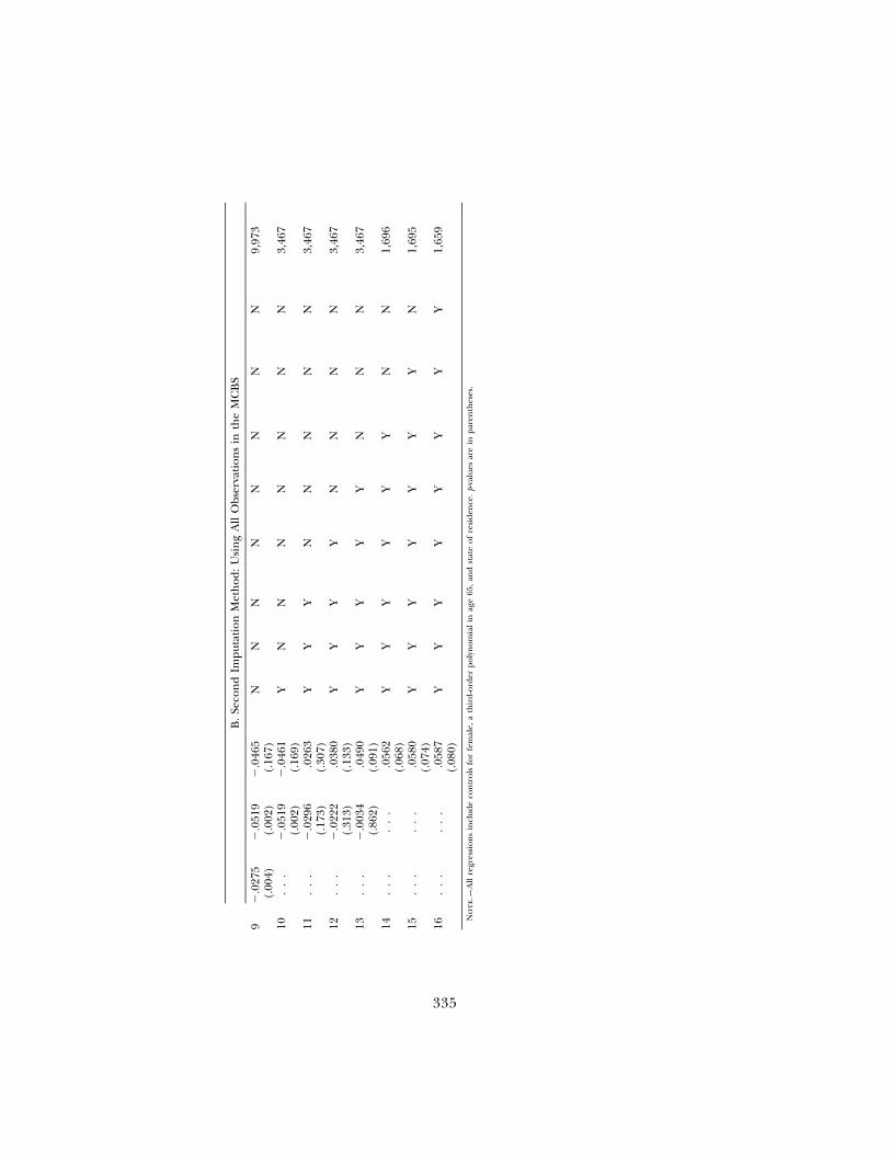
335
B.
Seco
nd
Impu
tati
onM
eth
od:
Usi
ng
All
Obs
erva
tion
sin
the
MC
BS
9�
.027
5(.
004)
�.0
519
(.00
2)�
.046
5(.
167)
NN
NN
NN
NN
9,97
3
10.
..
�.0
519
(.00
2)�
.046
1(.
169)
YN
NN
NN
NN
3,46
7
11.
..
�.0
296
(.17
3).0
263
(.30
7)Y
YY
NN
NN
N3,
467
12.
..
�.0
222
(.31
3).0
380
(.13
3)Y
YY
YN
NN
N3,
467
13.
..
�.0
034
(.86
2).0
490
(.09
1)Y
YY
YY
NN
N3,
467
14.
..
..
..0
562
(.06
8)Y
YY
YY
YN
N1,
696
15.
..
..
..0
580
(.07
4)Y
YY
YY
YY
N1,
695
16.
..
..
..0
587
(.08
0)Y
YY
YY
YY
Y1,
659
No
te.—
All
regr
essi
ons
incl
ude
con
trol
sfo
rfe
mal
e,a
thir
d-or
der
poly
nom
ial
inag
e65
,an
dst
ate
ofre
side
nce
.p-
valu
esar
ein
pare
nth
eses
.
336 journal of political economy
health expenditures. In rows 3 and 11 we report results from a regressionthat includes risk tolerance, the predicted variance, and the interactionbetween the two. The inclusion of these measures affects the coefficientestimate on .35 In the medium samples, the estimated coefficient onEj
remains negative but is now statistically indistinguishable from zero.Ej
In the small samples, the coefficient on reverses its sign from negativeEj
to positive, though it is statistically indistinguishable from zero.Notably, the estimated coefficient on the level of risk tolerance and
the interaction between variance and risk tolerance are bothVarj
negative. The latter is as we would expect. The probability of buyinginsurance increases with greater risk aversion, and more so for aperson who faces a higher variance of expenditures. According toour point estimates, at the mean level of in our sample, a one-Varj
standard-deviation increase in the risk tolerance measure decreases theprobability of purchasing Medigap by 6.7 percentage points. What ispuzzling, at least from the perspective of standard economic theory, isthat the coefficient on the variance term is negative. As the inter-Varj
action between variance and risk tolerance is also negative, this impliesthat individuals with higher uncertainty in their medical expendituresare less likely to purchase Medigap (with this negative effect being largerfor people who are more risk tolerant).
Remark 1. Strictly in terms of mechanics, the negative coefficientwe estimate for the variance term is not a surprise. To see this, noteVarthat because the inclusion of in the regression reduces the mag-Varnitude of the negative coefficient on , is in some sense acting asˆ E Vara “source” of advantageous selection. Thus it must satisfy the two prop-erties listed in Section III. Because increases with (i.e., those withˆVar Ehigher mean health expenditure also have high variance of health ex-penditure), it has to be the case that reduces the probability ofVarpurchasing Medigap in order for it to “act” as a source of advantageousselection.
Remark 2. A possible explanation within the standard expectedutility theory for the negative coefficient estimate on , with meanVarexpenditure held fixed, goes as follows: Consider a simple static modelEin which consumers face a loss of L with probability p. Then a mean-preserving spread implies reducing p while increasing L. Why mightsomeone with higher L (and lower p) demand less insurance? Underthe current U.S. institutional structure, Medicaid may cover catastrophiclosses, and emergency rooms are required to (and often do) treat theuninsured. Thus the incentives for purchasing Medigap may be lower
35 The bulk of the change in the coefficient on is attributable to the inclusion of aEj
control for the variance in health expenditure. For example, in results not shown here,adding just a control for variance in the smallest sample increases the coefficient on Ej
to .0370, with a p-value of .143.
sources of advantageous selection 337
for those with higher L (and lower p) because large losses are morelikely to be eligible for public-funded health care.
Remark 3. Several conventional departures from the expected util-ity theory postulated in the behavioral decision theory literature canalso explain the negative coefficient on variance. In such models, adecrease in p, with pL held fixed, could in fact reduce demand forinsurance. For example, in the rank-dependent utility model (see, e.g.,Quiggin 1982; Starmer 2000), the probability weights in expected utilitytheory are replaced by probability weighting functions. Say these func-tions down-weight low-probability events. Then, in a comparison of twopeople with equal pL, but where one has a large probability of smalllosses and the other has a very small probability of catastrophic losses,the latter person may in fact demand less insurance (because he or shechooses to engage in “wishful thinking” and largely ignore the smallchance of the catastrophic event).
Remark 4. Yet another possible behavioral explanation is that in-dividuals may underestimate the variance of their health expenditures.It is possible that, conditional on mean expenditures, those with highervariances will have a larger downward bias in their prediction of variance,reducing their demand for insurance.36
Remark 5. The above discussions have assumed that variance is afixed and exogenous trait of an individual. A final possibility is that itis instead endogenous. For example, the technology of health invest-ment may be such that the same behaviors that lead to poor healthcause both a higher mean and a higher variance in expenditures, aswell as leading people to purchase less insurance.
• As we include more variables from , reported respectively in rowsX j
4–8 and rows 12–16 for the two imputation methods, the coefficient oneventually becomes positive and statistically significant at the 5–10Ej
percent level. A key result is in row 6, where the inclusion of cognitiveability as a control variable causes the coefficient on predicted expen-diture to turn to positive .0758 with a p-value of .049. The most completespecification 8 implies that a $10,000 increase in predicted health ex-penditure increases the probability of buying Medigap by 7.8 percentagepoints. All the new variables we include shift the partial correlationX j
between health expenditure risk and Medigap coverage in a positivedirection.
Among all the variables in , cognition and income are distinctivelyX j
important in two senses: first, if only cognition or income is includedin , it substantially changes the estimated coefficient on ; and second,ˆX Ej j
when all variables in are included in the regression, both cognitionX j
36 Koufopoulos (2005) explores how overconfidence in risk perception might lead toadvantageous selection.
338 journal of political economy
and income stand out as significant predictors of Medigap purchase.For example, adding the cognition variables alone changes the coef-ficient on from �.057 (p-value .12) to �.012 (p-value .68); and in theEj
full regression that includes all elements of , a standard deviationX j
increase in just the TICS score is associated with a 5.4-percentage-pointincrease in the probability of purchasing a Medigap policy.37
Similarly, adding income variables alone changes the coefficient onfrom �.057 (p-value .12) to �.022 (p-value .45); and someone withEj
an annual income between $45,000 and $50,000 is 12 percentage pointsmore likely to purchase a Medigap policy than someone with an incomebetween $15,000 and $20,000. Thus, both cognition and income providesome important part of the explanation for the otherwise negative cor-relation between mean expenditure risk and insurance purchase.
In summary, these results indicate that sources of the advantageousselection we documented in Section VI include a number of factors—income, education, longevity expectations, and financial planning ho-rizon—that would typically enter a rich economic model of insurancepurchase. In addition, however, we find evidence that factors typicallyomitted from economic models, such as levels of cognitive ability andfinancial numeracy, are also important sources of advantageous selec-tion. (We will explore the pathways through which cognitive ability mayact as a source of advantageous selection below.) We find no evidence,however, that risk preferences, which the theoretical literature has fo-cused on and which are significant predictors of Medigap purchase, canexplain advantageous selection in this market. These findings are robustto the methods we use to impute expected medical expenditure and itsvariance.
Our study is, to the best of our knowledge, the first to provide directevidence on the sources of advantageous selection in health insurancemarkets; it is also the first study to identify a set of variables that aresufficient to explain away the negative correlation between ex posthealth expenditure and Medigap coverage documented in Section VIand obtain a positive partial correlation between health expenditurerisk and the level of insurance coverage.
Robustness.—In our working paper (Fang et al. 2006), we showed thatour findings regarding the sources of advantageous selection are robustto different choices regarding whether those with employer-providedhealth insurance are included, as well as alternative measures of healthexpenditure risk (i.e., potential Medigap expenditure as described inSec. VI.C) and alternative measures of the degree of uncertainty in
37 For reasons of space, these results are not presented here but are available from theauthors on request.
sources of advantageous selection 339
health expenditures (i.e., using the ratio of ninetieth and tenth per-centiles in place of the variance).
D. Pathways for Cognitive Ability as a Source of Advantageous Selection
Our analysis points to cognitive ability as an important source of ad-vantageous selection in the Medigap market. Because this factor is typ-ically omitted from economic models, we consider here potential path-ways through which cognitive ability may induce advantageous selection.This subsection is exploratory. Further research is needed to quantifythe importance of the postulated pathways.
• A first potential pathway through which cognitive ability may act asa source of advantageous selection is via its effect on individuals’ abilityto evaluate the costs and benefits of purchasing Medigap. This channelis consistent, for example, with earlier literature showing that manysenior citizens have difficulty understanding Medicare and Medigaprules; in particular, many fail to understand Medicare cost-sharing re-quirements (see, e.g., Cafferata 1984; McCall, Rice, and Sangl 1986;Davidson, Sofaer, and Gertler 1992; Harris and Keane 1998).38 The con-ceptual framework in Section III clarifies how this channel might work.Let (p, c) denote health risk and cognitive ability, respectively. Supposethat there is a negative correlation between c and p; that is, individualswith higher cognitive ability have lower health expenditure risk. Thenone particularly simple model of this channel would have a thresholdcognitive ability level below which individuals are simply unaware ofc*Medigap and therefore do not buy. Alternatively, might represent thec*cognitive ability level below which the costly effort required to determinethe optimal Medigap decision is too great. In this latter case, optimalrules of thumb or other psychological forces may lead consumers moreoften to choose the status quo of no Medigap.39 In either case, thosewith will purchase Medigap if it is worthwhile, and presumablyc 1 c*only those with high health expenditure risk, that is, , will choosep 1 p*to purchase Medigap. As a result, the set of individuals who purchaseMedigap insurance is given by , and theQ p {(p, c) : c ≥ c*, p ≥ p*}Medigap
set of individuals who do not purchase Medigap is given by. Because of the negativeQ p {(p, c) : c ! c*; or (c 1 c*, p ! p*)}No_Medigap
correlation in the population between c and p, such that p tends to be
38 There is also a literature showing that many consumers have difficulty understandinghealth insurance plans more generally. See, e.g., Gibbs, Sangl, and Burrus (1996), Isaacs(1996), Tumlinson et al. (1997), and Cunningham, Denk, and Sinclair (2001).
39 See, e.g., Iyengar and Lepper (2000), Iyengar and Jiang (2003), and Choi, Laibson,and Madrian (forthcoming) for evidence of the effect of complexity on the likelihood ofchoosing defaults and making “no choice.”
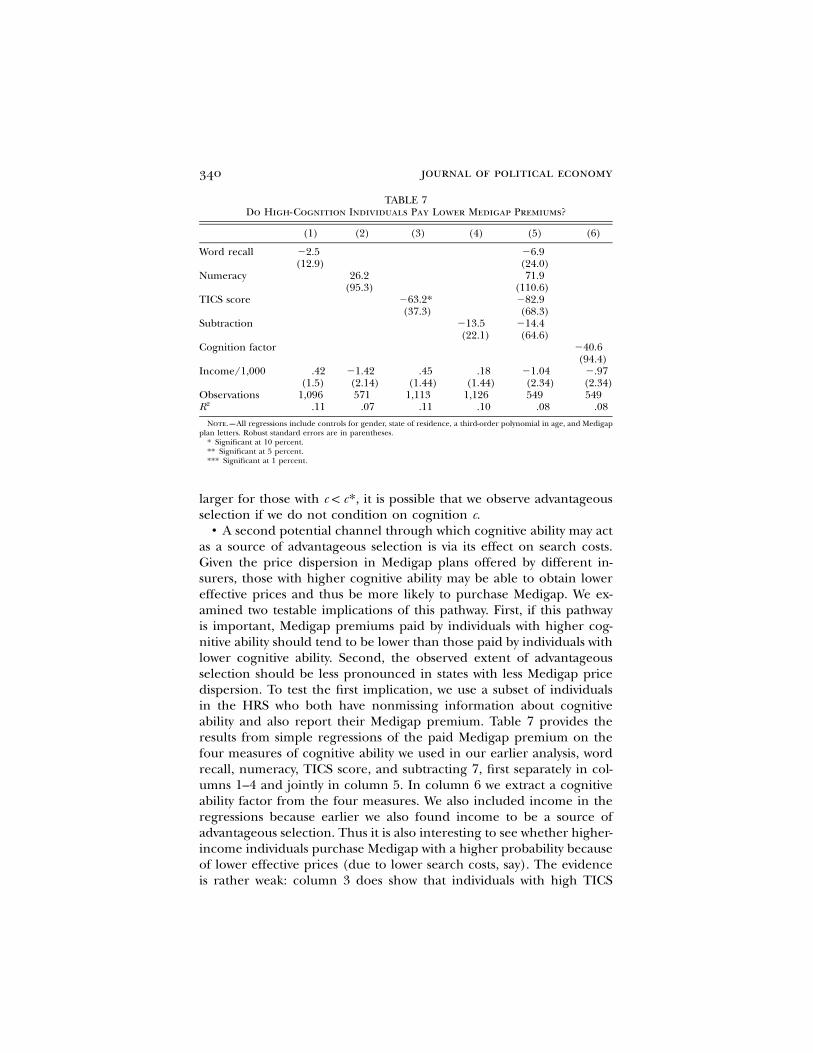
340 journal of political economy
TABLE 7Do High-Cognition Individuals Pay Lower Medigap Premiums?
(1) (2) (3) (4) (5) (6)
Word recall �2.5(12.9)
�6.9(24.0)
Numeracy 26.2(95.3)
71.9(110.6)
TICS score �63.2*(37.3)
�82.9(68.3)
Subtraction �13.5(22.1)
�14.4(64.6)
Cognition factor �40.6(94.4)
Income/1,000 .42(1.5)
�1.42(2.14)
.45(1.44)
.18(1.44)
�1.04(2.34)
�.97(2.34)
Observations 1,096 571 1,113 1,126 549 5492R .11 .07 .11 .10 .08 .08
Note.—All regressions include controls for gender, state of residence, a third-order polynomial in age, and Medigapplan letters. Robust standard errors are in parentheses.
* Significant at 10 percent.** Significant at 5 percent.*** Significant at 1 percent.
larger for those with , it is possible that we observe advantageousc ! c*selection if we do not condition on cognition c.
• A second potential channel through which cognitive ability may actas a source of advantageous selection is via its effect on search costs.Given the price dispersion in Medigap plans offered by different in-surers, those with higher cognitive ability may be able to obtain lowereffective prices and thus be more likely to purchase Medigap. We ex-amined two testable implications of this pathway. First, if this pathwayis important, Medigap premiums paid by individuals with higher cog-nitive ability should tend to be lower than those paid by individuals withlower cognitive ability. Second, the observed extent of advantageousselection should be less pronounced in states with less Medigap pricedispersion. To test the first implication, we use a subset of individualsin the HRS who both have nonmissing information about cognitiveability and also report their Medigap premium. Table 7 provides theresults from simple regressions of the paid Medigap premium on thefour measures of cognitive ability we used in our earlier analysis, wordrecall, numeracy, TICS score, and subtracting 7, first separately in col-umns 1–4 and jointly in column 5. In column 6 we extract a cognitiveability factor from the four measures. We also included income in theregressions because earlier we also found income to be a source ofadvantageous selection. Thus it is also interesting to see whether higher-income individuals purchase Medigap with a higher probability becauseof lower effective prices (due to lower search costs, say). The evidenceis rather weak: column 3 does show that individuals with high TICS
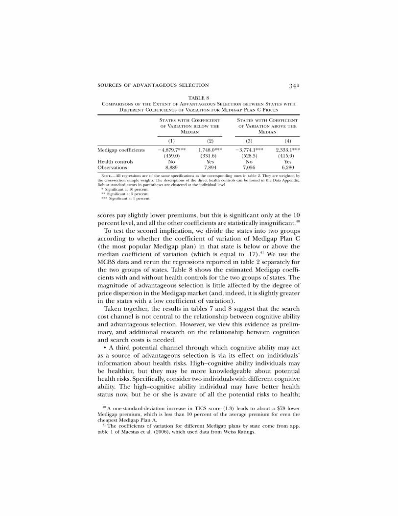
sources of advantageous selection 341
TABLE 8Comparisons of the Extent of Advantageous Selection between States with
Different Coefficients of Variation for Medigap Plan C Prices
States with Coefficientof Variation below the
Median
States with Coefficientof Variation above the
Median
(1) (2) (3) (4)
Medigap coefficients �4,879.7***(459.0)
1,748.0***(331.6)
�3,774.1***(528.5)
2,333.1***(415.0)
Health controls No Yes No YesObservations 8,889 7,894 7,056 6,280
Note.—All regressions are of the same specifications as the corresponding ones in table 2. They are weighted bythe cross-section sample weights. The descriptions of the direct health controls can be found in the Data Appendix.Robust standard errors in parentheses are clustered at the individual level.
* Significant at 10 percent.** Significant at 5 percent.*** Significant at 1 percent.
scores pay slightly lower premiums, but this is significant only at the 10percent level, and all the other coefficients are statistically insignificant.40
To test the second implication, we divide the states into two groupsaccording to whether the coefficient of variation of Medigap Plan C(the most popular Medigap plan) in that state is below or above themedian coefficient of variation (which is equal to .17).41 We use theMCBS data and rerun the regressions reported in table 2 separately forthe two groups of states. Table 8 shows the estimated Medigap coeffi-cients with and without health controls for the two groups of states. Themagnitude of advantageous selection is little affected by the degree ofprice dispersion in the Medigap market (and, indeed, it is slightly greaterin the states with a low coefficient of variation).
Taken together, the results in tables 7 and 8 suggest that the searchcost channel is not central to the relationship between cognitive abilityand advantageous selection. However, we view this evidence as prelim-inary, and additional research on the relationship between cognitionand search costs is needed.
• A third potential channel through which cognitive ability may actas a source of advantageous selection is via its effect on individuals’information about health risks. High–cognitive ability individuals maybe healthier, but they may be more knowledgeable about potentialhealth risks. Specifically, consider two individuals with different cognitiveability. The high–cognitive ability individual may have better healthstatus now, but he or she is aware of all the potential risks to health;
40 A one-standard-deviation increase in TICS score (1.3) leads to about a $78 lowerMedigap premium, which is less than 10 percent of the average premium for even thecheapest Medigap Plan A.
41 The coefficients of variation for different Medigap plans by state come from app.table 1 of Maestas et al. (2006), which used data from Weiss Ratings.
342 journal of political economy
the one with low cognitive ability thinks that there will be no morehealth shocks beyond what he or she already experienced. The firstindividual may be more likely to purchase Medigap than the second,thus leading to advantageous selection.42
Understanding the pathways for cognitive ability and other variablesto act as sources of advantageous selection has important policy impli-cations. If the first channel is important, it would suggest a role foreducational interventions to facilitate choice, or simplification of Medi-gap rules to make the cost-benefit calculations simpler (see, e.g., Harris2002); if the second channel is important, then pamphlets with detailedprice quotes (products that Weiss Ratings currently provides at a cost)directly sent to Medicare recipients may increase Medigap enrollment;if the third channel is important, it will call for yet a different kind ofinformation campaign, which is not about Medicare or Medigap, butabout various health risks the elderly may be facing.
V. Conclusion
In this paper we use data from the Medicare Current Beneficiary Surveyto provide strong evidence of advantageous selection in Medigap in-surance market. The first type of evidence comes from two sets of re-gressions. In one set, we regress total medical expenditure on Medigapstatus and control only for the determinants of price (gender, age, andstate of residence). We find that those with Medigap incur, on average,about $4,000 less in total medical expenditure than those without Medi-gap. In the second set of regressions, we regress total medical expen-diture on the determinants of price along with a rich set of controlsfor health status. Conditional on price and health, we find that thosewith Medigap incur about $2,000 more in medical expenditure, onaverage, than those without Medigap. These two sets of results can bereconciled only if those with better health are more likely to purchasesupplemental coverage, that is, if there is “advantageous selection.”These results are robust to different definitions of Medigap status andto separating the sample into male and female subsamples. We find thatthe magnitude of advantageous selection is larger for females than formales.
We then propose a simple empirical strategy to combine MCBS andHRS data and examine the sources of advantageous selection. Our find-ings indicate that these sources include factors, such as income, edu-cation, and planning horizons, that a rich economic model of insurance
42 We thank an anonymous referee for suggesting this potential pathway for cognitiveability to act as a source of advantageous selection. Coelho and de Meza (2007) also arguedthat individuals with different cognitive abilities may have different abilities to predict thelikelihood of illness, which will affect their insurance purchase.
sources of advantageous selection 343
purchase would typically accommodate. Interestingly, we find no evi-dence that variation in risk preferences, which is the primary focus ofthe theoretical literature on advantageous selection, explains the oth-erwise negative relationship between coverage and expenditure risk.Those who are less risk tolerant buy more insurance, but they are notparticularly healthy.
In addition, we find that measures of cognitive ability and financialnumeracy, which standard economic models do not accommodate, areimportant sources of advantageous selection; and we provide a prelim-inary exploration of the pathways through which cognitive ability mayact as a source of advantageous selection. Our findings also suggest thatheterogeneity in risk distributions, not merely expected levels of ex-penditure risk, should be included in models of asymmetric information.Specifically, we found that differences in the variance of health expen-diture, which standard models of insurance purchase ignore, are relatedboth to average expenditure risk and to insurance purchase. Our find-ings are robust to changes in the sample and the method of imputingexpected medical expenditure.
Finally, while advantageous selection in an insurance market can can-cel out the positive correlation between ex post risk and insurance cov-erage that arises in classic adverse selection models such as Rothschildand Stiglitz (1976), it is important to emphasize that this does not meanthere is no inefficiency in such a market. The policy implications ofmultidimensional selection models are an important topic for futureresearch.
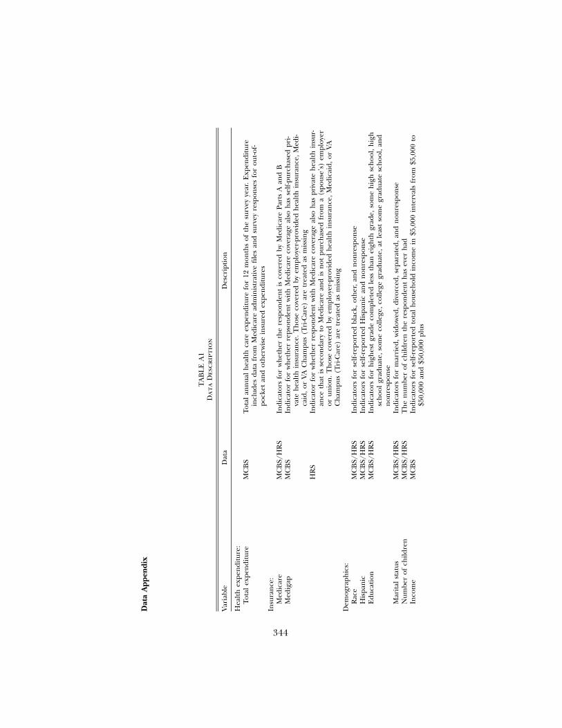
344
Dat
aA
ppen
dix
TA
BL
EA
1D
ata
Des
crip
tio
n
Var
iabl
eD
ata
Des
crip
tion
Hea
lth
expe
ndi
ture
:To
tal
expe
ndi
ture
MC
BS
Tota
lan
nua
lh
ealt
hca
reex
pen
ditu
refo
r12
mon
ths
ofth
esu
rvey
year
.E
xpen
ditu
rein
clud
esda
tafr
omM
edic
are
adm
inis
trat
ive
file
san
dsu
rvey
resp
onse
sfo
rou
t-of-
pock
etan
dot
her
wis
ein
sure
dex
pen
ditu
res
Insu
ran
ce:
Med
icar
eM
CB
S/H
RS
Indi
cato
rsfo
rw
het
her
the
resp
onde
nt
isco
vere
dby
Med
icar
ePa
rts
Aan
dB
Med
igap
MC
BS
Indi
cato
rfo
rw
het
her
reps
onde
nt
wit
hM
edic
are
cove
rage
also
has
self
-pur
chas
edpr
i-va
teh
ealt
hin
sura
nce
.Th
ose
cove
red
byem
ploy
er-p
rovi
ded
hea
lth
insu
ran
ce,M
edi-
caid
,or
VAC
ham
pus
(Tri
-Car
e)ar
etr
eate
das
mis
sin
gH
RS
Indi
cato
rfo
rw
het
her
resp
onde
nt
wit
hM
edic
are
cove
rage
also
has
priv
ate
hea
lth
insu
r-an
ceth
atis
seco
nda
ryto
Med
icar
ean
dis
not
purc
has
edfr
oma
(spo
use’
s)em
ploy
eror
unio
n.
Th
ose
cove
red
byem
ploy
er-p
rovi
ded
hea
lth
insu
ran
ce,M
edic
aid,
orVA
Ch
ampu
s(T
ri-C
are)
are
trea
ted
asm
issi
ng
Dem
ogra
phic
s:R
ace
MC
BS/
HR
SIn
dica
tors
for
self
-rep
orte
dbl
ack,
oth
er,
and
non
resp
onse
His
pan
icM
CB
S/H
RS
Indi
cato
rsfo
rse
lf-r
epor
ted
His
pan
ican
dn
onre
spon
seE
duca
tion
MC
BS/
HR
SIn
dica
tors
for
hig
hes
tgr
ade
com
plet
edle
ssth
anei
ghth
grad
e,so
me
hig
hsc
hoo
l,h
igh
sch
ool
grad
uate
,som
eco
llege
,co
llege
grad
uate
,at
leas
tso
me
grad
uate
sch
ool,
and
non
resp
onse
Mar
ital
stat
usM
CB
S/H
RS
Indi
cato
rsfo
rm
arri
ed,w
idow
ed,d
ivor
ced,
sepa
rate
d,an
dn
onre
spon
seN
umbe
rof
child
ren
MC
BS/
HR
ST
he
num
ber
ofch
ildre
nth
ere
spon
den
th
asev
erh
adIn
com
eM
CB
SIn
dica
tors
for
self
-rep
orte
dto
tal
hou
seh
old
inco
me
in$5
,000
inte
rval
sfr
om$5
,000
to$5
0,00
0an
d$5
0,00
0pl
us

345
HR
SSa
me
indi
cato
rsas
abov
e,ex
cept
inth
isca
sew
eus
ere
port
edas
wel
las
impu
ted
valu
esfo
rto
tal
hou
seh
old
inco
me.
Impu
tati
ons
are
thos
ege
ner
ated
byR
and.
See
htt
p://
hrs
onlin
e.is
r.um
ich
.edu
/met
a/ra
nd/
ran
dhrs
e/ra
ndh
rse.
pdff
orde
tails
ofth
eim
puta
tion
Wor
kst
atus
MC
BS/
HR
SIn
dica
tors
ifcu
rren
tly
wor
kin
gfo
rpa
yan
dfo
rn
onre
spon
seH
ealt
h:
Self
-rep
orte
dM
CB
S/H
RS
Indi
cato
rsfo
rse
lf-r
epor
ted
hea
lth
exce
llen
t,ve
rygo
od,
good
,an
dfa
irH
eigh
tM
CB
S/H
RS
Self
-rep
orte
dh
eigh
t,in
inch
es,
and
hei
ght
squa
red
Bod
ym
ass
inde
xM
CB
S/H
RS
Self
-rep
orte
d[w
eigh
t(k
g)]/
[hei
ght
(m)2 ]
Eve
ra
smok
erM
CB
S/H
RS
Indi
cato
rif
resp
onde
nt
has
“eve
rsm
oked
”to
bacc
oC
urre
nt
smok
erM
CB
S/H
RS
Indi
cato
rif
resp
onde
nt
now
smok
esto
bacc
oan
dfo
rn
onre
spon
seD
iagn
oses
MC
BS/
HR
SIn
dica
tors
for
ifa
doct
orh
asev
erto
ldth
ere
spon
den
th
e/sh
eh
asar
thri
tis,
hig
hbl
ood
pres
sure
,di
abet
es,(
non
skin
)ca
nce
r,lu
ng
dise
ase,
hea
rtat
tack
,ch
ron
ich
eart
dise
ase,
stro
ke,
psyc
hia
tric
illn
ess,
Alz
hei
mer
’sdi
seas
e,br
oken
hip
,an
dfo
rea
chdi
agn
osis
,n
onre
spon
seTr
eatm
ents
MC
BS/
HR
SIn
dica
tors
for
resp
onde
nt
ever
hav
ing
cata
ract
surg
ery
ora
hea
rin
gai
d(I
nst
rum
enta
l)A
DL
sM
CB
S/H
RS
Indi
cato
rsfo
rif
are
spon
den
th
asat
leas
tso
me
diffi
cult
yw
alki
ng
2–3
bloc
ks,s
toop
ing,
reac
hin
gov
erh
ead,
lifti
ng
10lb
s.,d
ress
ing,
wal
kin
gat
all,
bath
ing,
eati
ng,
gett
ing
out
ofa
chai
r,us
ing
the
toile
t,da
ilyliv
ing,
prep
arin
gm
eals
,sh
oppi
ng,
usin
gth
ete
le-
phon
e,m
anag
ing
mon
eyan
dbi
lls,a
nd
for
non
resp
onse
Hel
pw
ith
inst
rum
enta
lA
DL
sM
CB
S/H
RS
Indi
cato
rsfo
rif
are
spon
den
tre
ceiv
esh
elp
dres
sin
g,w
alki
ng
atal
l,ba
thin
g,ea
tin
g,ge
t-ti
ng
out
ofa
chai
r,us
ing
the
toile
t,pr
epar
ing
am
eal,
shop
pin
g,us
ing
the
tele
phon
e,or
man
agin
gm
oney
and
bills
,an
dfo
rn
onre
spon
seR
isk
atti
tude
s:R
isk
tole
ran
ceH
RS
Est
imat
eof
risk
tole
ran
cefr
omK
imba
llet
al.
(for
thco
min
g),u
sin
gre
spon
ses
toh
ypo-
thet
ical
inco
me
gam
bles
from
1992
and
1994
Cog
nit
ion
:W
ord
reca
llH
RS
Var
iabl
esre
cord
ing
the
num
ber
ofw
ords
reca
lled
from
alis
tof
10,
both
imm
edia
tely
afte
rth
elis
tw
asre
adan
dse
vera
lm
inut
esla
ter
TIC
Ssc
ore
HR
STe
leph
one
Inte
rvie
wfo
rC
ogn
itiv
eSt
atus
:n
umbe
rof
corr
ect
answ
ers
ona
test
ofkn
owle
dge,
lan
guag
e,an
dor
ien
tati
on.Q
uest
ion
sin
clud
en
amin
gob
ject
s,vo
cabu
lary
ques
tion
s,an
dba
sic
know
ledg
esu
chas
the
U.S
.pr
esid
ent’
sn
ame
Subt
ract
ion
HR
SN
umbe
rof
tim
esre
spon
den
tca
nsu
btra
ctth
en
umbe
r7
sequ
enti
ally
,sta
rtin
gfr
om10
0

TA
BL
EA
1(C
ontin
ued)
Var
iabl
eD
ata
Des
crip
tion
Num
erac
yH
RS
Num
ber
ofco
rrec
tan
swer
sto
“wor
dpr
oble
ms”
ofdi
visi
onan
dm
ulti
plic
atio
non
topi
csof
prob
abili
ty,c
ompo
und
inte
rest
,an
ddi
visi
onof
asse
ts;a
sked
only
in20
02E
xpec
tati
ons:
Lon
gevi
tyH
RS
Mos
tre
cen
tan
swer
toth
equ
esti
on“W
hat
isth
epe
rcen
tch
ance
you
will
live
to75
orm
ore?
”Pl
ann
ing
hor
izon
:Fi
nan
cial
HR
SIn
dica
tors
for
wh
eth
erth
ere
spon
den
t’s
mos
tim
port
ant
peri
odfo
rpl
ann
ing
savi
ng
and
spen
din
gis
the
nex
tfe
wm
onth
s,th
en
ext
year
,th
en
ext
few
year
s,th
en
ext
5–10
year
s,or
mor
eth
an10
year
s
sources of advantageous selection 347
References
Arrow, Kenneth. 1963. “Uncertainty and the Welfare Economics of MedicareCare.” A.E.R. 53 (December): 941–73.
Banthin, Jessica S., and Amy K. Taylor. 2001. “HMO Enrollment in the UnitedStates: Estimates Based on Household Reports, 1996.” MEPS Research Find-ings no. 15, Agency for Healthcare Research and Quality, Rockville, MD.
Barsky, Robert B., F. Thomas Juster, Miles Kimball, and Matthew D. Shapiro.1997. “Preference Parameters and Behavioral Heterogeneity: An ExperimentalApproach in the Health and Retirement Study.” Q.J.E. 112 (May): 537–79.
Cafferata, Gail L. 1984. “Knowledge of Their Health Insurance Coverage by theElderly.” Medical Care 22 (September): 835–47.
Cardon, James H., and Igal Hendel. 2001. “Asymmetric Information in HealthInsurance: Evidence from the National Medical Expenditure Survey.” Rand J.Econ. 32 (Autumn): 408–27.
Cawley, John, and Tomas Philipson. 1999. “An Empirical Examination of Infor-mation Barriers to Trade in Insurance.” A.E.R. 89 (September): 827–46.
Charles, Kerwin, and Erik Hurst. 2003. “The Correlation of Wealth across Gen-erations.” J.P.E. 111 (December): 1155–82.
Chiappori, Pierre-Andre. 2001. “Econometric Models of Insurance under Asym-metric Information.” In Handbook of Insurance, edited by Georges Dionne.Boston: Kluwer.
Chiappori, Pierre-Andre, Bruno Jullien, Bernard Salanie, and Francois Salanie.2006. “Asymmetric Information in Insurance: General Testable Implications.”Rand J. Econ. 37 (Winter): 783–98.
Chiappori, Pierre-Andre, and Bernard Salanie. 2000. “Testing for AsymmetricInformation in Insurance Markets.” J.P.E. 108 (February): 56–78.
Choi, James J., David Laibson, and Brigitte C. Madrian. Forthcoming. “Reducingthe Complexity Costs of 401(k) Participation through Quick Enrollment�.”In Developments in the Economics of Aging, edited by David A. Wise. Chicago:Univ. Chicago Press.
CMS (Centers for Medicare and Medicaid Services). 2005. Choosing a MedigapPolicy: A Guide to Health Insurance for People with Medicare. Baltimore: U.S. Dept.Health and Human Services.
Coelho, Marta, and David de Meza. 2007. “Self Deception, Self Selection, SelfDestruction: Experimental Evidence against Adverse Selection.” Manuscript,London School Econ.
Cohen, Alma. 2005. “Asymmetric Information and Learning: Evidence from theAutomobile Insurance Market.” Rev. Econ. Statis. 87 (June): 197–207.
Cohen, Alma, and Liran Einav. 2007. “Estimating Risk Preferences from De-ductible Choice.” A.E.R. 97 (June): 745–88.
Cox, Donald F., and Christopher Hogan. 1997. “Biased Selection and MedicareHMOs: Analysis of the 1989–1994 Experience.” Medical Care Res. and Rev. 54(September): 259–85.
Cunningham, Peter J., Charles Denk, and Michael Sinclair. 2001. “Do ConsumersKnow How Their Health Plan Works?” Health Affairs 20 (March/April): 159–66.
Davidson, Bruce, Shoshanna Sofaer, and Paul Gertler. 1992. “Consumer Demandand Biased Selection in the Demand for Coverage Supplementing Medicare.”Soc. Sci. and Medicine 34 (9): 1023–34
de Meza, David, and David C. Webb. 2001. “Advantageous Selection in InsuranceMarkets.” Rand J. Econ. 32 (Summer): 249–62.
Desmond, Katherine A., Thomas Rice, and Peter D. Fox. 2006. “Does Greater

348 journal of political economy
Medicare HMO Enrollment Cause Adverse Selection into Medigap?” HealthEcon., Policy and Law 1 (1): 3–21.
Dionne, Georges, Christian Gourieroux, and Charles Vanasse. 2001. “Testing forEvidence of Adverse Selection in the Automobile Insurance Market: A Com-ment.” J.P.E. 109 (April): 444–53.
Ettner, Susan L. 1997. “Adverse Selection and the Purchase of Medigap Insuranceby the Elderly.” J. Health Econ. 16 (October): 543–62.
Fang, Hanming, Michael P. Keane, and Dan Silverman. 2006. “Sources of Ad-vantageous Selection: Evidence from the Medigap Insurance Market.” Work-ing Paper no. 12289 (June), NBER, Cambridge, MA.
Finkelstein, Amy, and Kathleen McGarry. 2006. “Multiple Dimensions of PrivateInformation: Evidence from the Long-Term Care Insurance Market.” A.E.R.96 (September): 938–58.
Finkelstein, Amy, and James Poterba. 2004. “Adverse Selection in InsuranceMarkets: Policyholder Evidence from the U.K. Annuity Market.” J.P.E. 112(February): 183–208.
———. 2006. “Testing for Adverse Selection with ‘Unused Observables.’” Man-uscript, Dept. Econ., Massachusetts Inst. Tech.
Gibbs, Deborah A., Judith A. Sangl, and Barri Burrus. 1996. “Consumer Per-spectives on Information Needs for Health Plan Choice.” Health Care FinancingRev. 18 (Fall): 55–73.
Harris, Katherine M. 2002. “Can High Quality Overcome Consumer Resistanceto Restricted Provider Access? Evidence from a Health Plan Choice Experi-ment.” Health Services Res. 37 (June): 551–71.
Harris, Katherine M., and Michael P. Keane. 1998. “A Model of Health PlanChoice: Inferring Preferences and Perceptions from a Combination of Re-vealed Preference and Attitudinal Data.” J. Econometrics 89 (November): 131–57.
Hemenway, David. 1990. “Propitious Selection.” Q.J.E. 105 (November): 1063–69.
Hurd, Michael D., and Kathleen McGarry. 1997. “Medical Insurance and theUse of Health Care Services by the Elderly.” J. Health Econ. 16 (April): 129–54.
Isaacs, Stephen L. 1996. “Consumers’ Information Needs: Results of a NationalSurvey.” Health Affairs 15 (Winter): 31–41.
Iyengar, Sheena S., and Wei Jiang. 2003. “Choosing Not to Choose: The Effectof More Choices on Retirement Savings Decisions.” Manuscript, ColumbiaUniv.
Iyengar, Sheena S., and Mark Lepper. 2000. “When Choice Is Demotivating: CanOne Desire Too Much of a Good Thing?” J. Personality and Soc. Psychology 79(December): 995–1006.
Jullien, Bruno, Benard Salanie, and Francois Salanie. 2007. “Screening RiskAverse Agents under Moral Hazard.” Econ. Theory 30 (January): 151–69.
Kaiser Family Foundation. 2005. Medicare Chart Book. Washington, DC: KaiserFamily Found.
Kan, Kamhon. 2003. “Residential Mobility and Job Changes under Uncertainty.”J. Urban Econ. 54 (November): 566–86.
Keane, Michael P. 2004. “Modeling Health Insurance Choice Using the Het-erogeneous Logit Model.” Manuscript, Yale Univ.
Kezdi, G., and R. J. Willis. 2005. “Who Becomes a Stockholder? Expectations,Subjective Uncertainty, and Asset Allocation.” Manuscript, Univ. Michigan.
Khandker, Rezaul K., and Lauren A. McCormack. 1996. Enrollment and Utilization

sources of advantageous selection 349
across Medicare Supplemental Plans. Report submitted to the Health Care Fi-nancing Admin. Washington, DC: Center Health Econ. Res.
———. 1999. “Medicare Spending by Beneficiaries with Various Types of Sup-plemental Insurance.” Medical Care Res. and Rev. 56 (June): 137–55.
Khwaja, Ahmed. 2005. “The Dynamic Trade-off between Medical ExpenditureInsurance, Moral Hazard and Mortality Risk: A Life Cycle Analysis of the Effectsof Medicare on Individual Health Incentives and Health Outcomes.” Manu-script, Fuqua School Bus., Duke Univ.
Kimball, Miles S., Claudia R. Sahm, and Matthew D. Shapiro. Forthcoming.“Using Survey-Based Risk Tolerance.” J. American Statis. Assoc.
Koufopoulos, Kostas. 2005. “Asymmetric Information, Heterogeneity in Risk Per-ceptions and Insurance: An Explanation of a Puzzle.” Manuscript, LondonSchool Econ.
Lewin Group. 2001. “Restricting Underwriting and Premium Rating Practicesin the Medigap Market: The Experience of Three States.” Report no. 2001-01. Washington, DC: AARP, Public Policy Inst.
Lillard, Lee A., and Jeannette Rogowski. 1995. “Does Supplemental Private In-surance Increase Medicare Costs?” Working Paper no. 95-16, Rand Corp.,Santa Monica, CA.
Lusardi, Annamaria. 1998. “On the Importance of the Precautionary SavingMotive.” A.E.R. Papers and Proc. 88 (May): 449–54.
Maestas, Nicole, Mathis Schroeder, and Dana Goldman. 2006. “Price Variationin Markets with Homogeneous Goods: The Case of Medigap.” Working Paperno. 504, Rand Corp., Santa Monica, CA.
McCall, Nelda, Thomas Rice, and Judith Sangl. 1986. “Consumer Knowledge ofMedicare and Supplemental Health Insurance Benefits.” Health Services Res.20 (February): 633–57.
Pauly, Mark V. 1974. “Overinsurance and Public Provision of Insurance: TheRoles of Moral Hazard and Adverse Selection.” Q.J.E. 88 (February): 44–62.
Puelz, Robert, and Arthur Snow. 1994. “Evidence on Adverse Selection: Equi-librium Signaling and Cross-Subsidization in the Insurance Market.” J.P.E. 102(April): 236–57.
Quiggin, John. 1982. “A Theory of Anticipated Utility.” J. Econ. Behavior andOrganization 3 (December): 323–43.
Ridder, Geert, and Robert Moffitt. 2007. “The Econometrics of Data Combi-nation.” In Handbook of Econometrics, vol. 6A, edited by James J. Heckman andEdward E. Leamer. Amsterdam: Elsevier.
Robst, John. 2006. “Estimation of a Hedonic Pricing Model for Medigap Insur-ance.” Health Res. and Educational Trust 41 (December): 2097–2113.
Rothschild, Michael, and Joseph E. Stiglitz. 1976. “Equilibrium in CompetitiveInsurance Markets: An Essay on the Economics of Imperfect Information.”Q.J.E. 90 (November): 629–49.
Schmidt, Lucie. Forthcoming. “Risk Preferences and the Timing of Marriageand Childbearing.” Demography.
Starmer, Chris. 2000. “Developments in Non–Expected Utility Theory: The Huntfor a Descriptive Theory of Choice under Risk.” J. Econ. Literature 38 (June):332–82.
Tumlinson, Anne, Hannah Bottigheimer, Peter Mahoney, Elliot Stone, and AnnHendricks. 1997. “Choosing a Health Plan: What Information Will ConsumersUse?” Health Affairs 16 (May/June): 229–38.
Wilson, Charles. 1977. “A Model of Insurance Markets with Incomplete Infor-mation.” J. Econ. Theory 16 (December): 167–207.

350 journal of political economy
Wolfe, John R., and John H. Goddeeris. 1991. “Adverse Selection, Moral Hazardand Wealth Effects in the Medigap Insurance Market.” J. Health Econ. 10 (4):433–59.