NBER WORKING PAPER SERIES

SOURCES OF ADVANTAGEOUS SELECTION: EVIDENCEFROM THE MEDIGAP INSURANCE MARKET

Hanming FangMichael P. Keane

Dan Silverman

Working Paper 12289http://www.nber.org/papers/w12289

NATIONAL BUREAU OF ECONOMIC RESEARCH1050 Massachusetts Avenue

Cambridge, MA 02138June 2006

We thank Pierre-Andr e Chiappori, Alessandro Lizzeri, Jim Poterba, Bernard Salani e, Aloysius Siow, andespecially Amy Finkelstein, as well as seminar participants at Brown, Concordia, Duke/UNC, FederalReserve Bank of New York, Queens, Toronto, Virginia, Wharton and Yale for many helpful suggestions. Weare grateful to Mike Chernew for the access to, and Tami Swenson for clarification of, the Medicare CurrentBeneficiary Survey data. All remaining errors are our own. Fang and Silverman gratefully acknowledgefinancial support from the Economic Research Initiative on the Uninsured. The views expressed herein arethose of the author(s) and do not necessarily reflect the views of the National Bureau of Economic Research.

©2006 by Hanming Fang, Michael P. Keane and Dan Silverman. All rights reserved. Short sections of text,not to exceed two paragraphs, may be quoted without explicit permission provided that full credit, including© notice, is given to the source.

Sources of Advantageous Selection: Evidence from the Medigap Insurance MarketHanming Fang, Michael P. Keane and Dan SilvermanNBER Working Paper No. 12289June 2006JEL No. D82, G22, I11

ABSTRACT

We provide strong evidence of advantageous selection in the Medigap insurance market, and analyzeits sources. Using Medicare Current Beneficiary Survey (MCBS) data, we find that, conditional oncontrols for the price of Medigap, medical expenditures for senior citizens with Medigap coverageare, on average, about $4,000 less than for those without. But, if we condition on health,expenditures for seniors on Medigap are about $2,000 more. These two findings can only bereconciled if those with less health expenditure risk are more likely to purchase Medigap, implyingadvantageous selection. By combining the MCBS and the Health and Retirement Study (HRS), weinvestigate the sources of this advantageous selection. These include income, education, longevityexpectations and financial planing horizons, as well as cognitive ability. Once we condition on allthese factors, seniors with higher expected medical expenditure are indeed more likely to purchaseMedigap. Surprisingly, risk preferences do not appear to be a source of advantageous selection. Butcognitive ability emerges as a particularly important factor, consistent with a view that many seniorcitizens have difficulty understanding Medicare and Medigap rules.

Hanming FangYale UniversityDepartment of Economics37 Hillhouse AvenueP.O. Box 208264New Haven, CT 06520-8264and NBERhanming.fang@yale.edu

Michael P. KeaneDepartment of EconomicsYale UniversityBox 208264New Haven, CT 06520-8264michael.keane@yale.edu

Dan SilvermanInstitute for Advanced StudyEinstein DrivePrinceton, NJ 08540and NBERdansilv@umich.edu

1 Introduction

Asymmetric information is central to modern economic models of insurance pioneered by Ar-

row (1963) and Pauly (1974). The classic equilibrium models developed by Rothschild and Stiglitz

(1976) and Wilson (1977) assume that potential insurance buyers have one-dimensional private

information regarding their risk type. They choose from a menu of contracts, specifying the price

and amount of coverage, the one best suited to their type. These simple models predict a positive

correlation between insurance coverage and ex post realizations of loss. The reason is simply ex

ante adverse selection: the “bad risks” (i.e., those relatively likely to suffer a loss) have an incentive

to buy more insurance. Allowing for ex post moral hazard only strengthens the positive correla-

tion between coverage and ex post loss. This “positive correlation property” of classic asymmetric

information models (see Chiappori and Salanie 2000) forms the basis for empirical tests of asym-

metric information in several recent papers.1 Interestingly, these papers, which examine a variety

of important insurance markets, generally fail to find empirical support for the positive correlation

property (see Section 2 for details).

Indeed, it is often found that, conditional on pricing information, those who buy more insurance

tend to be relatively good risks – a phenomenon that has been called “advantageous selection.”

Some researchers have speculated that multi -dimensional private information can explain this phe-

nomenon.2 For example, de Meza and Webb (2001), postulate that individuals have private in-

formation about both their risk type and their risk aversion. Selection based on risk aversion is

advantageous if: (1) the more risk averse buy more insurance coverage; and (2) the more risk

averse have lower risks. Then, failure to condition on risk aversion may mask the expected positive

correlation between insurance coverage and ex post risk that exists in one-dimensional models.3 Of

course, while the prior literature has emphasized risk aversion as the prime suspect,4 it is not the

only potential source of advantageous selection. More generally, selection based on any private in-

formation item γ is advantageous if γ is positively correlated with insurance coverage but negatively

1Chiappori, Jullien, Salanie and Salanie (2005) generalize this empirical prediction to a large class of models where

the insurance market is competitive and the risk aversion of the insured is public knowledge, assuming a suitably

modified notion of positive correlation between risk occurrence and coverage. Chiappori (2000) provides a useful

survey of the theoretical and empirical literature up to that date.

2See, e.g., the concluding discussions in Chiappori and Salanie (2001) and Finkelstein and Poterba (2004).

3The first verbal description of this phenomenon in the economics literature appears to be Hemenway (1990, 1992),

who used the term “propitious selection.”

4The notable exception is Finkelstein and McGarry (2006) who also found advantageous selection on wealth in

their study of the long term care insurance market.

1

correlated with risk (see Section 3 for details). Furthermore, γ need not be private information,

but could also include observables that insurers are not permitted to use in setting prices.

While prior work has speculated that advantageous selection based on unobservables accounts

for the empirical failure of the “positive correlation property,” it has not provided direct evidence

to support this conjecture.5 Nor has it provided direct evidence on the source (or sources) of

advantageous selection, be it risk aversion and/or something else.

In this paper, we study the advantageous selection phenomenon using data from the Medicare

supplemental or “Medigap” insurance market. A “Medigap” policy is health insurance sold by

a private insurer to fill “gaps” in coverage of the basic Medicare plan (e.g. co-pays, prescription

drugs).6 We show that the Medigap market is characterized by advantageous selection: conditional

on the determinants of price, those who purchase supplemental insurance tend to be healthier

than those who do not. More importantly, we go beyond prior research to investigate several

potential sources of this advantageous selection. We find that these sources include standard

factors such as income, education, longevity expectations and financial planing horizons, as well

as less conventionally modelled variables including cognitive ability and financial numeracy. Once

we condition on all these factors, individuals with higher expected medical expenditures are indeed

more likely to purchase Medigap insurance.

Interestingly, while the theoretical literature has emphasized risk preferences as a potential

source of advantageous selection, we find little evidence in support of that hypothesis. Direct

measures of risk tolerance are significant predictors of Medigap insurance purchase but do not

contribute much to advantageous selection.7 Rather, cognitive ability and income emerge as far

more important sources of advantageous selection.

Our finding that cognitive ability is an important source of advantageous selection is consistent

with earlier literature showing that many senior citizens have difficulty understanding Medicare

and Medigap rules (see, e.g., Cafferata (1984), McCall et al. (1986), Davidson et al. (1992), Harris

and Keane (1999)). In particular, it appears that many fail to understand Medicare cost sharing

requirements. There is also a literature showing that many consumers have difficulty understanding

5Finkelstein and McGarry (2006), which we discuss in more detail in Section 2, use preventive health care as a

proxy for risk preference, and find indirect evidence of advantageous selection based on risk preference.

6See Section 4 for more details about the Medicare program and the Medigap insurance market.

7In this regard, our results are consistent with Cohen and Einav (2005) who estimate a structural model of

automobile insurance deductible choice, and use it to infer both accident risk and risk aversion. They find risk type is

positively correlated with risk aversion, contrary to what is required for risk aversion to be a source of advantageous

selection. The evidence in Cohen and Einav is, however, indirect, as neither risk or risk aversion are directly measured.

2

health insurance plans more generally. See, e.g., Gibbs et al. (1996), Isaacs (1996), Tumlinson et

al. (1997), Cunningham et al. (2001). Our results imply that senior citizens with relatively low

cognitive ability also tend to have relatively high health expenditure risk and low probability of

buying Medigap (even conditional on income and price). This may suggest a role for educational

interventions to facilitate choice (see, e.g., Harris (2002)).

The Medigap market is ideal for studying advantageous selection because the coverage and

pricing of Medigap policies are highly regulated by the U.S. government. First, in all but three

States, insurance companies can only sell ten standardized Medigap policies. Second, within the

six month Medigap open enrollment period – which starts when an individual is both older than 65

and enrolled in Medicare Part B – an insurer cannot deny Medigap coverage, or place conditions

on a policy, or charge more for pre-existing health conditions. Indeed Robst (2001) finds that

the average Medigap premium an individual faces depends almost exclusively on his/her State of

residence, age and gender. Thus, we do not need to worry that the sources of advantageous selection

we have identified (e.g., income, cognition, etc.) might influence prices because they are potentially

observed by insurers.8

Another key feature of the Medigap market is that it is intimately linked to the Medicare

program, so one can obtain detailed administrative data on diagnoses, treatments and expenditures.

We exploit this link and use in our analysis the Medicare Current Beneficiary Survey (MCBS), which

combines survey data and Medicare administrative records. The Medicare administrative data on

medical expenditure provide perhaps the most accurate measure of health expenditure risk of any

commonly available data set. Though the MCBS itself does not contain detailed information about

risk aversion and other potential sources of advantageous selection, the Health and Retirement

Study (HRS), a longitudinal data set covering a large sample of the Medicare eligible population,

has information about such variables. Our empirical strategy uses the MCBS and HRS jointly to

examine the sources of advantageous selection.

The remainder of the paper is structured as follows. Section 2 reviews related literature; Section

3 presents a simple theoretical framework to illustrate the idea of advantageous selection; Section

4 provides some detailed background about Medicare and the Medigap insurance market; Section

5 describes the MCBS and HRS data sets used in our analysis; Section 6 provides direct and

indirect evidence of advantageous selection using the MCBS data; Section 7 examines the sources

8As shown in the theoretical analysis of Julien, Salanie and Salanie (2005), the non-competitiveness of the Medigap

insurance market is a necessary condition for the multi-dimensional private information to manifest itself in terms of

a non-positive correlation between ex post risk and coverage.

3

of advantageous selection by combining the MCBS and HRS, and presents our main results; Section

8 presents several robustness checks on our results; Section 9 briefly discusses the conditions under

which our estimates also provide a lower bound on the magnitude of moral hazard (or price effect)

of Medigap insurance coverage; and finally, Section 10 concludes.

2 Related Literature

Empirical Tests for the Presence of Asymmetric Information. Standard equilibrium mod-

els of insurance markets predict a positive correlation between insurance coverage and ex post risk

(Chiappori, Jullien, Salanie and Salanie 2005). This positive correlation property has been tested in

several recent studies, for a variety of markets. Cawley and Philipson (1999) use four data sources

including the HRS and the Asset and Health Dynamics Among the Oldest Old (AHEAD) to test

for positive correlation between self-perceived or objective mortality risk and the probability of

purchasing life insurance. To the contrary, they find the mortality rate of U.S. males who purchase

life insurance is below that of the uninsured, even when controlling for many factors such as income

that may be correlated with life expectancy.

The evidence from the auto insurance market is more ambiguous. Chiappori and Salanie (2000)

show that accident rates are lower for young French drivers who choose comprehensive automo-

bile insurance than for those opting for the legal minimum coverage, even after controlling for

observable characteristics known to automobile insurers (though the difference is not statistically

significant). On the other hand, there is a literature that supports the presence of adverse selec-

tion in the choice of contractual forms, including deductibles and co-payments etc. For example,

Puelz and Snow (1994) argued, in the context of automobile collision insurance, that in an adverse

selection equilibrium, individuals with lower risk will choose a contract with a higher deductible,

and contracts with higher deductibles should be associated with lower average prices for coverage.

They find evidence in support of each of these predictions using individual data from an automobile

insurer in Georgia.9 Similarly, Cohen (2005), using data from Israel, finds that new auto insurance

customers choosing a low deductible tend to have more accidents, leading to higher total losses to

the insurer.10

9However, see Chiappori and Salanie (2000) and Dionne, Gourieroux and Vanasse (2001) for some criticisms of

the Puelz and Snow study.

10Moreover, she finds this correlation exists among experienced new customers (those with 3 or more years of

driving experience), but not among inexperienced new customers (those with little or no driving experience). This

suggests learning is involved in the origin of private information.

4

Cardon and Hendel (2001) use a different approach to test for information asymmetries in

health insurance markets. They estimate a structural model of health insurance and health care

choices using data on single individuals from the National Medical Expenditure Survey. They

find that estimated price and income elasticities, as well as demographic differences, can explain

the expenditure gap between the insured and the uninsured. Thus they judge the role of adverse

selection to be economically insignificant.11

Finkelstein and Poterba (2004) use a unique individual level data set on annuities from the

U.K. and find systematic relationships between ex post mortality and annuity characteristics, such

as the timing of payments and the possibility of payments to the annuitants’ estate. But they do

not find evidence of substantive mortality differences by annuity size.

Finkelstein and McGarry (2006). Our paper is most closely related to recent work by Finkel-

stein and McGarry (2006), who study selection based on multi-dimensional private information in

the long-term care (LTC) insurance market. Using the AHEAD data they find a negative (though

statistically insignificant) correlation between LTC coverage in 1995 and use of nursing home care

in the period between 1995-2000, even after controlling for insurers’ assessment of a person’s risk

type - (weakly) suggesting the presence of advantageous selection. However, the 1995 AHEAD also

contains the subjective probability assessment “What do you think are the chances that you will

move to a nursing home in the next five years?” This variable is known by the insured and the

econometrician, but unobserved by the insurer, so it cannot be used in setting prices. Finkelstein

and McGarry (2006) find this subjective risk assessment is positively correlated with both LTC

coverage and nursing home use in 1995-2000, even after controlling for insurers’ risk assessment,

suggesting the presence of adverse selection based on private information about risk type.12

What makes the Finkelstein and McGarry (2006) paper similar to ours is that they develop

a proxy for risk aversion, using information on whether respondents undertake various types of

preventive health care.13 They find that people who are more risk averse by this measure are

11In their structural model, Cardon and Hendel (2001) assume that individuals have identical preferences.

12Recently, Finkelstein and Poterba (2006) proposed such use of characteristics of insurance buyers that are ob-

servable to the econometrician but not used by insurers in setting prices as a general strategy to test for asymmetric

information in insurance markets. If one can find one or more such observables that are correlated with both the

insurance coverage and the risk occurrence, then one rejects the null hypothesis of symmetric information.

13The potential preventive health care measures they include are: whether the individual had a flu shot, had a

blood test for cholesterol, checked her breast for lumps monthly, had a mammogram or breast x-ray, had a Pap smear

and had a prostate screen.

5

both more likely to own LTC insurance and less likely to enter a nursing home – consistent with

advantageous selection based on risk aversion.

To summarize, Finkelstein and McGarry (2006) find that the overall correlation between LTC

insurance coverage and use of long-term care is negative but insignificant. They conclude that

multidimensional private information explains this result, since they find adverse selection based

on the subjective risk assessment and advantageous selection based on their proxy for risk aversion,

and it seems these two factors may roughly cancel on net.

Our paper complements and extends Finkelstein and McGarry (2006) in several ways. First,

we examine a much larger insurance market, the Medigap market. More than half the over age 65

respondents in our HRS data purchased a Medigap policy. In contrast, the LTC insurance market is

very small (only about 10 percent of the elderly in the AHEAD had LTC insurance). Besides being

a very large and important market, we feel the Medigap market has several important advantages

for studying asymmetric information.

First, studying the Medigap market allows us to employ a different method of inference about

the presence of advantageous selection. The key point is that regulation effectively precludes price

discrimination on the basis of health risk. Thus, we can consider the effect on the estimated

relationship between Medigap coverage and ex-post risk of conditioning on a rich set of health

information that is, by law, private to consumers. This gives us a much richer set of “private” risk

measures than the single subjective risk assessment used by Finkelstein and McGarry (2006).

Second, we examine not just one possible source of advantageous selection (i.e., risk aversion),

but several other potential sources as well. For this purpose, we use HRS information on other

objects of special theoretical interest such as longevity expectations, planning horizons, cognition

and financial numeracy, etc. Third, rather than using behavioral proxies for risk aversion, we

exploit the direct measures of risk aversion contained in the HRS.

Finally, the Medigap market has the key virtue that ex post health expenditure risk (i.e.,

health expenditure itself) can be quite accurately measured using the MCBS. This dataset contains

comprehensive health expenditure data for a large sample of the entire Medicare population, from

age 65 until death. It also contains very extensive health measures, enabling one to form accurate

measures of ex post expenditure conditional on age and health.14

14In contrast, available LTC data sets do not contain large samples of respondents at the oldest ages, when many

episodes of nursing home care occur. Since many nursing home admissions occur in the few years/months before

death, the best measure of ex post risk for LTC is whether one eventually uses nursing home care prior to death, not

whether one uses it over some particular time period. Since many of the respondents in the AHEAD data used by

Finkelstein and McGarry (2006) are still alive, their measure of ex post risk - whether the respondent used a nursing

6

Literature on Adverse Selection in the Medigap Market. Our paper is also related to a

literature that looks for evidence of adverse selection in the Medigap market. Wolfe and Goddeeris

(1991) examine this issue using data from the Retirement History Survey, a longitudinal survey of

recent retirees conducted by Social Security Administration between 1969 and 1979. They used self

reported health and self reported expenditure measures, the latter including total medical bills for

hospital, physician and prescription expenditures, including any amount paid by insurance. They

found that respondents with better self-reported health were more likely to purchase supplemental

private insurance. But those with private insurance also incurred higher expenditures on hospital

stays, physician care and prescription drugs (though this difference was statistically insignificant).

Hurd and McGarry (1997) used the first wave of AHEAD to examine how health insurance

influences the use of health care services by the elderly. They found that those with more compre-

hensive insurance tend to use more health care services (as measured by number of hospital and

doctor visits), controlling for self-reported health indicators.15 However, they also found little rela-

tionship between observable health measures and either the propensity to hold or purchase health

insurance, indicating little importance of adverse selection.

Khandker and McCormack (1996) estimated multinomial logit models of insurance choice and

found that individuals reporting better health were significantly more likely to enroll in private

supplemental plans. This is consistent with advantageous selection, although self reported health

does not necessarily correspond to ex post expenditure.

In contrast, Ettner (1997), using MCBS 1991, found little evidence of variation in the probability

of purchasing private insurance by health status.16 She also found that Medicare beneficiaries

with supplemental policies had higher total Medicare and physician expenditures than those with

employer-provided policies, even after controlling for observable differences. She interprets this as

evidence of adverse selection under the assumption that selection into employer provided coverage

is random. We view this assumption as implausible. Moreover, those with employer-sponsored

health insurance may be subject to different rules regarding whether Medicare is the primary payer

for various services. Such issues are important because Ettner (1997) examined only Medicare

reimbursed expenditure.

home between 1995 and 2000 – may be relatively incomplete. The AHEAD sample represents the population born

before 1924, and who were at least 76 by the year 2000; but many are quite far from their time of death. According

to life-table estimates, those alive at age 75 in 2000, had on average 11.4 more years to live (Vital Statistics, 2004).

15They did not report results without controlling for measured health.

16Lillard and Rogowski (1995), using the Panel Study of Income Dynamics (PSID), also found little evidence of

adverse selection for supplemental insurance.

7

Finally, Khandker and McCormack (1999), using MCBS 1991 and 1993, found that those with

supplemental private insurance tended to incur higher levels of Medicare reimbursed spending,

particularly Part B services. However, because Medigap plans cover Medicare co-pays, they reduce

the out-of-pocket price of Medicare covered services. Thus, it is possible that those with Medigap

incur higher Medicare reimbursed expenditures, while nonetheless incurring less total health care

spending. (Indeed, Section 6.1 provides evidence consistent with this view.) Conversely, those

with basic Medicare alone may incur more total expenditures, despite smaller Medicare reimbursed

expenditures, because they spend more out of pocket. Thus, we would argue that, to study adverse

selection in Medigap, a better measure of health expenditure risk is total medical expenditure, not

just expenditure reimbursed by Medicare or Medigap.17

3 Multi-dimensional Private Information and Advantageous Se-

lection

It is now well understood that, given multi-dimensional private information, the correlation

between ex post risk realizations and coverage may be negative, zero, or positive - see, Henmenway

(1990, 1992), de Meza and Webb (2001), Araujo and Moreira (2001) and Jullien, Salanie and

Salanie (2005). These papers all focus on private information about risk aversion as the source of

advantageous selection. In this section, we first follow the literature and illustrate this idea using

risk aversion in a partial equilibrium example; then, anticipating our main empirical focus, we

expand our definition of advantageous selection to include selection based on other types of private

information.

Risk Aversion as the Source of Advantageous Selection Consider an individual over age

65 (so she has basic Medicare as a baseline level of coverage). She has a constant relative risk

aversion utility function

u (y) =y1−γ

1− γ,

where γ is the relative risk aversion parameter. She has wealth Y > 0, and faces a risk of incurring

a health expenditure shock (over and above what is covered by basic Medicare) of L > 0 with

17Unfortunately, the waves of the MCBS data used in Khandker and McCormack’s (1999) analysis only contained

Medicare claim data, but did not contain information about total health cost, including beneficiary out-of-pocket

cost as well as expenses paid by supplementary insurers. We are grateful to Tami Swenson for the clarification on

these data issues.

8

probability p ∈ [0, 1] .18 For simplicity, assume that the individual can choose to purchase Medigap

insurance at a premium m that will reduce the out-of-pocket expenditure to 0. Her expected utilities

from buying and not buying Medigap are respectively given by

VB (p, γ) = u (Y −m) + e

VN (p, γ) = pu (Y − L) + (1− p) u (Y ) .

where e is a fixed cost of buying Medigap (i.e., the time and psychic costs of applying), that has

a logistic distribution in the population, independent of p and γ. The probability the individual

purchases Medigap is then given by the logit expression:

Q (p, γ) =exp [VB (p, γ)]

exp [VB (p, γ)] + exp [VN (p, γ)](1)

Simple algebra shows that Q (p, γ) is increasing in p and γ.19 That is, more risky and more risk

averse individuals are more likely to purchase Medigap.

Now suppose that in the population there is a joint distribution over individuals’ private types

(p, γ) given by F, and let the CDF of risk aversion conditional on risk type p be Fγ|p (·|·) . If we

do not control for risk aversion γ and look only at the relationship between risk-type p and the

probability of purchasing Medigap, we obtain the marginal probability expression:

Q (p) =∫

Q (p, γ) dFγ|p (γ|p) . (2)

If p and γ are negatively correlated, then Q (p) may or may not increase in p.

We can also compare the average health shock risk p for those with and without Medigap

insurance. The average risk among those with Medigap insurance is given by

AB =∫

Q (p, γ) pdF (p, γ)∫Q (p, γ) dF (p, γ)

, (3)

where the denominator is the measure of individuals who purchase Medigap, and the numerator is

the expected number of health shocks that occur to those who purchase Medigap. Similarly, the

18We assume away the price effect, also called “moral hazard” as in Cutler and Zeckhauser (1999), by assuming

the expenditure level L does not depend on health insurance status.

19Note that, the sign of ∂Q/∂p is the same as the signs of ∂ (VB − VN ) /∂p, which is given by:

∂ (VB − VN )

∂p= u (Y )− u (Y − L) > 0.

To show that Q (p, γ) is increasing in γ, it is easier to use the fact that, for any γ′ > γ, there exists a strictly concave

and increasing function v (·) such that u (y; γ′) ≡ v (u (y; γ)).

9

average risk among those without Medigap is

AN =∫

[1−Q (p, γ)] pdF (p, γ)∫[1−Q (p, γ)] dF (p, γ)

. (4)

Chiappori and Salanie’s (2000) test for asymmetric information is a test of whether AB > AN .

However, if p and γ are negatively correlated, it is possible that AB ≤ AN despite the presence of

asymmetric information.

The above example is merely illustrative, as we only analyze individuals’ insurance purchase

decisions assuming a particular equilibrium (i.e., a particular menu of insurance options), and do

not analyze the full equilibrium in which insurance companies may compete by offering different

insurance contracts.20 However, this simple example captures the idea that, when individuals differ

in both risk type and risk aversion, it is possible that those who purchase more coverage may on

average be lower risk (if there is negative correlation between risk aversion and risk type).

Sources of Advantageous Selection: General Discussion The above illustration showed

how private information about risk aversion can be a source of advantageous selection into insurance.

We will now generalize this concept. For this purpose, we again let p denote the probability of

a health expenditure shock. But we now interpret γ as any private information that may affect

agents’ probability of purchasing Medigap Q (p, γ) . Now instead of deriving Q (p, γ) explicitly as we

did when γ was interpreted as risk aversion, we take the probability of Medigap purchase Q (p, γ)

as the reduced-form entity of focus. Viewed from this perspective, we state the general properties

for a private information item γ to act as a source of advantageous selection as follows:

Property 1: γ is positively correlated with insurance coverage, i.e., Q (p, γ) is increasing in γ;

Property 2: γ is negatively correlated with risk p.

Under these two conditions, the average probability of insurance purchase for a given risk type

p, namely Q (p) as defined in (2), may not be monotonic in p; and the ranking of AB and AN ,

defined respectively by (3) and (4), can go either way. It is important to emphasize the assumed

negative correlation between γ and risk p may arise either exogenously or endogenously (in the

20We refer the reader to Julien, Salanie and Salanie (2005) for a formal equilibrium analysis of the case when the

insurance market is not competitive, and Chiappori, Julien, Salanie and Salanie (2005) for the case when the market

is competitive. The latter paper shows that, when the insurance market is competitive in the sense that profits

are not increasing in coverage, a suitably modified version of the positive correlation property still holds even with

multi-dimensional private information.

10

sense that the would-be-insured with a higher γ may take an action to reduce p). For our purpose

this distinction is unimportant.21

In our empirical analysis, we first provide, in Section 6, evidence that is akin to “AB < AN ,”

that is, the health risk occurrence for those with Medigap insurance is lower than those without

Medigap insurance, suggesting the existence of advantageous selection. Then in Section 7, we

examine the sources of advantageous selection, that is, we look for elements of γ that may account

for the earlier finding that AB < AN .

4 Background on Medicare and Medigap

4.1 Medicare

Medicare is the primary health insurance program for most seniors in the United States. All

Americans age 65 and older who have, or whose spouses have, paid Medicare taxes for more than

40 quarters are eligible. The original Medicare Plan consisted of two parts.22 Part A, the hospital

insurance program, covers inpatient hospital, skilled nursing facility, and some home health care.

Almost all retirees are automatically enrolled in Part A when they turn 65 and there are no

premiums paid for this coverage. For the first 60 days of a hospital stay, Medicare pays all covered

costs except a deductible, which equalled $912 in 2005. For days 61 through 90 Medicare requires

a co-pay that was $228 per day in 2005. For days 91-150 this co-pay rose to $456 per day. Hospital

stays beyond 150 days are not covered at all by Medicare. For “skilled nursing facility” care, the

coinsurance amount is about $114 per day for days 21 through 100 each benefit period, but no

coverage is provided beyond the 100th day in the benefit period.23 That is, Medicare covers short

nursing home stays (up to 100 days) for acute episodes, but does not cover long term care.

Medicare Part B (also called Medicare Insurance) covers Medicare eligible physician services,

outpatient hospital services, certain home health services, and durable medical equipment. Part

B enrollees have to pay a monthly premium, which was $67 in 2004. Almost all people choose

21See Culter, Finkelstein and McGarry (2006) for a simple model in which more risk averse individuals take actions

to reduce risk, thus endogenously generating a negative correlation between risk aversion and risk.

22For details, see Centers for Medicare and Medicaid Services (2005), pages 55-64. The basic Medicare plan is

available everywhere in the country. Some areas also offer what are now called Medicare Advantage Plans, which are

managed care plans (either HMOs or PPOs, i.e., preferred provider organizations). In 2001, approximately 15% of

Medicare beneficiaries were enrolled in such Medicare HMOs. See Keane (2004) for more discussion.

23Note that a skilled nursing facility is a nursing home. It provides both long term care and short term care while

a person recovers from an acute episode.

11

to enroll in Part B when they turn 65.24 Under Part B, individuals were responsible for a $110

deductible in 2005 and face a 20% co-pay payment for all Medicare-approved services after exceeding

the deductible. Until the recent introduction of “Part D,” which provides limited drug coverage,

Medicare did not cover prescription drugs.

4.2 Medigap

As is clear from above, Medicare leaves seniors at significant risk of health care expenditures. To

insure Medicare beneficiaries against some of that risk, private insurance companies sell “Medigap”

policies that cover some of the co-pays, deductibles and uncovered expenses, i.e. the “gaps,” in

the basic Medicare plan. Since 1990, by Federal law, Medigap policies are standardized into ten

plans, “A” through “J,” each representing a different constellation of benefits. The basic plan, A,

covers all co-pays for hospital stays longer than 60 days, and all co-pays for physician visits and

outpatient care (but not the deductible). All other plans offer these basic benefits, and more. Plan

B, for example, also covers the deductible ($912 in 2005) for hospital stays shorter than 60 days;

Plan C, which is the most popular, also covers co-pays for skilled nursing facilities, the Medicare

Part B deductible and provides foreign travel emergency coverage. Plan J adds to this, among

other things, prescription drug benefits (with a $3000 annual limit in 2004). While not all Medigap

policies are offered in every state, almost every state has a provider which offers the basic plan.25

If an insurer offers any Medigap policy, by law it must offer at least the basic plan.

In addition to being regulated with respect to quality, Medigap pricing and coverage are reg-

ulated in ways that tend to amplify the asymmetries of information favoring the insured. Most

important, Medigap policies are required by law to have an open enrollment period. This six month

open enrolment period begins after the first day of the first month an individual is both age 65

or older and enrolled in Medicare Part B. During this period, insurers cannot deny Medigap cov-

erage, delay coverage, or price coverage based on pre-existing conditions.26 Instead, during open

enrollment, insurers effectively price only on age, gender and state of residence.27 Moreover, these

24A person is automatically enrolled at age 65 if they have previously applied for Social Security Old Age Benefits.

25The exceptions are Massachusetts, Minnesota and Wisconsin which have received waivers that allow them to

offer somewhat different standardized plans.

26Moreover, even after open enrollment, so long as the would-be insured has had Medigap coverage for the past 6

months, enrollment in a different plan offered by the same company is guaranteed by law. When a consumer does

switch Medigap plans, the price of the policy may depend on the age at purchase, but coverage cannot be denied.

27Some insurance companies offer menus of Medigap policy options that may help to discriminate among those

with varying health risks. To our knowledge, the pricing comes in only three forms: 1) “age-issued policies” with a

12

insurance policies are required by law to be guaranteed renewable. That is, beneficiaries may not

be dropped from policies so long as they continue the timely payment of the contracted premiums.

It is also important to note that in some (mostly urban) areas, participants of both Medicare A

and B may enroll in Medicare HMOs, which may or may not charge an extra premium. About 60

percent of the Medicare HMO enrollees do not pay an extra premium. Rather, they exchange re-

strictions on their choices for medical treatment for additional coverage similar to that provided by

typical Medigap policies.28 For this reason, they are discouraged, though not precluded, from pur-

chasing additional Medigap insurance policies.29 Participation in a Medicare HMO is not restricted

by a previous lapse in coverage, unlike Medigap.

5 Data

5.1 Medicare Current Beneficiary Survey (MCBS)

Our analysis relies on two large data sets, the MCBS and HRS. The MCBS began in Septem-

ber 1991, and is a continuous panel survey of a nationally representative sample of the Medicare

population.30 Beneficiaries sampled from Medicare enrollment files (or appropriate proxies) are

interviewed in person, three times a year, using computer-assisted personal interviewing. All the

MCBS survey data are linked to Medicare claims and other administrative data. The final file

consists of survey, administrative, and claims data, and thus provides a comprehensive view of

respondents’ heath care costs and use.

The central goal of the MCBS is to determine expenditures and sources of payment for all

services used by Medicare beneficiaries, including co-payments, deductibles, and uncovered services.

This is important, since our focus is on the total health expenditure, i.e. the combined expenditures

flat premium that depends only on inflation and age at the date of purchase, 2) “age-attained policies” that have a

premium that starts lower than age-issued policies and rises on a predictable schedule as the beneficiary ages, and 3)

“community rated” policies whose premiums do not depend either on age at purchase or age attained.

28There is substantial evidence of favorable selection into Medicare HMOs (see Keane (2004) for a survey). There

is a strong consensus in the literature that this selection - rather than greater efficiency in providing services - is the

primary reason they have lower per patient costs than basic Medicare

29See page 5 of Center for Midicare and Medicaid Services (2004), which states: “If you’re in a Medicare Advantage

Plan, you don’t need a Medigap policy because Medicare Advantage Plans generally cover many of the same benefits

that a Medigap policy would cover, like extra days in the hospital after you used the number of days that Medicare

pays for.”

30See http://www.cms.hhs.gov/mcbs/ for more details. A supplemental sample is added annually in the

September-December round to replenish sample cells depleted by refusals and death.

13

that were covered by Medicare, other public insurance, private insurance, or paid out-of-pocket.

In addition, the MCBS also contains extensive information on the health and demographics of

respondents, and whether respondents have supplemental insurance. The Data Appendix provides

a detailed description of how the variables used in our analysis are constructed.

An important problem we confront in our empirical analysis is that the MCBS does not contain

information on many potential sources of advantageous selection. Conversely, the HRS does not

contain information on health expenditures. Thus, our strategy is to use the MCBS to estimate

the relationship between total health expenditure and a rich set of health variables. We then use

this estimated relationship to form expected health expenditures, Ei, for each HRS respondent.

We discuss the imputation procedure in Section 7.1.

5.2 Health and Retirement Study (HRS)

The HRS began as a panel survey of a nationally representative sample of people aged 51 to

61 in 1992, including their spouses, with oversamples of blacks, hispanics and residents of Florida.

This original cohort of 12,654 respondents has been re-interviewed every other year since. In 1998

the sample was supplemented with both older and younger cohorts. Our interest in those over age

65 leads us to limit our analysis to health and insurance data from the 2000 and 2002 waves of the

original HRS, the latest years for which a final version of the data is available.31

The HRS is particularly well-suited to a study of advantageous selection in Medigap insurance.

It contains detailed information about current and past health status of respondents, along with

rich data on their insurance choices and health care costs. The health information includes both

self-reported health and a very large set of objective measures, such as diseases diagnosed, and a

list of activities the respondent has difficulty performing.32 The insurance data include information

on where the insurance was acquired, its premiums, and its coverage. A detailed description of the

health and insurance information that we use is provided in the Data Appendix.

The HRS also contains high quality information about economic and demographic variables,

including education, income, wealth and cognition. In addition, the HRS is distinctive in its

attention to variables central to economic theory, including measures of risk aversion, longevity

31Because we use only the 2000 and 2002 waves of the HRS, we only use the 2000 and 2001 waves of the MCBS in

our main analysis, though we use lagged health measures from the 1999 MCBS in several specification checks.

32For our purposes, it is important that the health information contained in the HRS and MCBS be very similar.

This is crucial if we are to use the MCBS data to impute expected expenditures of HRS respondents, as we describe

in Section 7.1.

14

expectations, and financial planning horizons. The following sections describe these theoretically

important measures in greater detail.

5.2.1 Measures of Risk Preference

Risk preferences are central to theories of advantageous selection. Beginning in the first wave in

1992, the HRS asked (subsamples of) respondents a series of questions regarding their risk attitudes.

These respondents were first asked the following question:

“Suppose that you are the only income earner in the family, and you have a good job

guaranteed to give you your current (family) income every year for life. You are given

the opportunity to take a new and equally good job, with a 50-50 chance it will double

your (family) income and a 50-50 chance that it will cut your (family) income by a

third. Would you take the new job?”

If the answer to the first question is “yes,” the interviewer continues with the following question:

“Suppose the chances were 50-50 that it would double your (family) income, and 50-50

that it would cut it in half. Would you still take the new job?”

But, if the answer to the first question is “no,” the interviewer instead continues with the question:

“Suppose the chances were 50-50 that it would double your (family) income and 50-50

that it would cut it by 20 percent. Would you then take the new job?”

The responses to these questions place respondents into four, ordered risk categories: e.g., a person

who says “no“ to both questions is in category I (unwilling to risk any income cuts), while a person

who says “yes“ to both questions is in category IV (willing to risk a 50% cut in income). In Wave 2,

a randomly selected sub-sample answered the same sequence of questions, supplemented to include

jobs with risks of 10% and 75% declines in income.

A number of studies have used these measures of risk preferences and found them to be sig-

nificant predictors of risk-taking behavior both in the HRS and in the Panel Study of Income

Dynamics. See, for example, Barsky et al. (1997) on smoking, drinking and insurance purchase,

Lusardi (1998) on wealth accumulation, Charles and Hurst (2003) and Kimball et al. (2005) on

portfolio choice, Kan (2003) on residential and job mobility, and Schmidt (2006) on the timing of

fertility and marriage. Assuming that an individual’s responses to these hypothetical income gam-

bles are error-prone reflections of his/her fixed, constant relative risk aversion preferences, Kimball

15

et al. (2005) estimate the risk tolerance for each respondent in the HRS by maximum likelihood.

In the bulk of our analysis, we use their estimates to form our measures of risk aversion (see their

Table 6).

5.2.2 Expectations and Planning Horizons

Longevity expectations may also play an role in determining health insurance choices, though

the net effect of a higher longevity expectation on investment in health is theoretically ambiguous.

Those who expect to live longer may want to spend more now on their health as such investment will

pay dividends over a longer horizon (see Khwaja 2005). Thus, they would demand more insurance.

On the other hand, the marginal value of additional current health investment may be lower when a

long life already seems likely. The HRS collects detailed information about longevity expectations.

Our focus is on the response to the question, asked of all respondents age 65 and younger, and

repeated in every HRS wave, “What is (percent chance) you will live to 75 or more?” In our

analysis, we use the most recent available response to this question as our measure of longevity

expectations.33

Like expectations for longevity, the length of financial planning horizons (which presumably

reflects both uncertainty and the subjective rate of time discount) may influence insurance choices.

Here, the effect seems unambiguous, as those with longer horizons would be more willing to pay

larger immediate costs (premiums) to avoid expected future costs. The HRS also collects informa-

tion on financial planning horizons. Specifically, respondents in Wave 1 were asked:34

“In deciding how much of their (family) income to spend or save, people are likely to

think about different financial planning periods. In planning your (family’s) saving and

spending, which of the time periods listed in the booklet is most important to you [and

your (husband/wife/ partner)]? 1. Next few months, 2. Next year, 3. Next few years,

4. Next 5-10 years, 5. Longer than 10 years.”

We use indicator variables for each of these four responses in Wave 1 as our measures of the

33This question presumably measures longevity expectations with error, and may reflect both beliefs about longevity

and the degree of certainty about those beliefs. Evidence consistent with both error and uncertainty about beliefs is

found in the heaping of responses around focal response such as zero, fifty and, to a lesser extent, one hundred. See

Kezdi and Willis (2005) for a thorough discussion of these measures.

34This question was also asked, at random, of one out of ten respondents in Waves 4 and 5, but was not asked

of anyone age 65 and older in Wave 6. Of the 11,626 respondents who answered this question in Wave 1, just 821

answered it again in Wave 4 and 941 in Wave 5.

16

respondent’s financial planning horizon.

5.2.3 Measures of Cognition

Our measure of a person’s cognition combines his/her performance on four different tests/questions:

word recall, a Telephone Interview for Cognitive Status (TICS) score, subtraction, and numeracy.

These scores may proxy for an individual’s degree of economic “rationality,” i.e. his/her ability to

think through the costs and benefits of Medigap insurance. There is a large body of literature show-

ing that many of the elderly have difficulty understanding the basic Medicare entitlement, and/or

the features of supplemental insurance (see, e.g., Harris and Keane 1999 for empirical evidence and

Keane 2004 for a survey of the literature, much of which we cited in the introduction).

5.3 Medigap Insurance Status

Both the MCBS and HRS contain detailed information about respondents’ health insurance

choices. Specifically, each reports if the respondent is covered by Medicare, Parts A and B, and

whether that coverage is provided by a Medicare Advantage Plan (HMO/PPO). We also know if the

respondent had supplemental coverage and, if so, its premium and its source. Given that our goal is

study the decision to buy supplemental insurance, our sample should include only people with the

following characteristics: (1) they should be covered by basic Medicare (parts A and B), (2) they

should not have access to free (or heavily subsidized) supplemental coverage provided by a former

employer, or Medicaid, or some other government agency (e.g., the Veterans Administration). That

is, we want to limit the sample to people who would have to pay more than a nominal premium to

obtain supplemental coverage.

Our main empirical analysis is based on two alternative rules for sample inclusion and two

alternative indicators for Medigap status. Both samples include only respondents covered by basic

Medicare. In the first sample, we delete anyone covered by employer-provided supplemental health

insurance, Medicaid or other government insurance (e.g., VA insurance). Then, we define Medigap

status as equal to one if the respondent has purchased additional private insurance that is secondary

to Medicare.

The second sample retains respondents who have employer provided supplemental insurance,

provided they must pay at least $500 per year in premiums for that insurance. Then, we again

define Medigap status as equal to one if the respondent has purchased private insurance that is

secondary to Medicare, but this time including the employer provided insurance for which they pay

at least $500 in premiums.

17

Below, we separately report results using both definitions of Medigap status. To preview, none

of the results, either qualitatively or quantitatively, depends on which definition of Medigap status

we use. For our main analysis, we choose to code Medicare HMO enrollees as simply having basic

Medicare because, as we mentioned earlier, 60 percent of Medicare HMO enrollees do not pay any

extra premium. Thus their decision to enroll in a Medicare HMO is often really a trade-off between

restrictions on provider choice vs. additional coverage for the gaps in Medicare, not a decision to

pay for additional coverage. However in Section 8 we also report results where we code Medicare

HMO plan members in different ways. The qualitative results do not depend on whether we treat

Medicare HMO members as having “Medigap,” or instead drop them from the analysis.

5.4 Measures of Health and Medical Expenditure Risk

Both the MCBS and HRS have detailed measures of observable health.35 For our empirical

analysis, however, we need to summarize those health variables into a uni-dimensional measure of

health expenditure risk. That is, while we consider extension of classic models of adverse selection to

include multi-dimensional private information, we continue within the classical tradition of viewing

both health risk and the level of insurance coverage as one-dimensional constructs.36

For our measure of ex post health expenditure risk, we use “Total Medical Expenditure,” which

corresponds to the variable pamttot in the MCBS. This variable is constructed by CMS from a

variety of sources, including Medicare administrative records and survey responses.37 In calculating

pamttot, CMS includes, for any health care event identified either from the survey respondent or

from the respondent’s Medicare file, payments from 11 potential sources: Medicare fee-for-service,

Medicare HMOs, Medicaid, employer-based private health insurance, individually purchased private

35See the category “Health” in the data appendix for details.

36By doing this we abstract from the following sort of possibility: suppose a person is relatively healthy overall, but

chooses a Medigap plan because it has good coverage of expenses of treating a particular chronic condition from which

he/she suffers. If such cases were common, it might appear that Medigap participants had lower than average total

medical costs - advantageous selection - when in fact they are buying Medigap to cover costs of particular conditions.

This scenario seems implausible for two reasons: First, why would people with certain chronic conditions tend to be

healthier than the average person in the population in other ways? Second, it is ruled out by the legal restrictions on

what Medigap plans must cover. That is, as we discussed earlier, by law Medigap plans must cover various co-pays

and deductibles not covered by basic Medicare, so they can reasonably be thought of as simply providing “more”

coverage in a uni-dimensional level of coverage framework. Medigap plans cannot be structured to cover or include

particular health conditions.

37See MCBS public use documentation on “Cost and Use” Sections 3 and 5 for more details. This documentation

is available online at http://www.cms.hhs.gov/apps/mcbs/.

18

health insurance, private insurance managed care, private insurance with unknown sources, the VA

and other public insurance, out-of-pocket payments and uncollected liability. Thus, the variable

pamttot comes as close as is possible to measuring total health expenditure from all sources.

An important question is whether total medical expenditure is indeed the most relevant measure

of health expenditure risk when a would-be-insured contemplates whether to purchase Medigap.

One argument in favor of treating total medical expenditure as the relevant risk is that Medigap

policies by law cover broad ranges of expenditure not covered by Medicare (i.e., medicare deductibles

and co-pays, prescription drugs). A person in worse health would typically tend to have greater

expenditure risk in all of these areas. Thus, to a good approximation, Medigap plans can reasonably

be thought of a simply providing “more” coverage in a uni-dimensional health risk framework.

On the other hand, a more accurate measure of the incentive to purchase Medigap would

be expected Medigap covered expenditure. Ideally if we could identify all itemized charges an

individual experienced in a year, we could determine the amount of reimbursement that he/she

would receive under basic Medicare vs. under various Medigap plans. Two limitations of our data

preclude this approach. First, we do not have itemized medical bills; second, almost all health

questions in both data sets cover health stocks, i.e., whether an individual has ever had certain

treatments or diagnoses. Nonetheless, we also report results from an alternative measure of health,

which is we call “Potential Medigap Expenditure.” This is “Total Medical Expenditure” minus that

part which is reimbursed by Medicare and other government insurance (see Section 8.1.1). This

should reasonably approximate the medical expenditure that could have been covered by Medigap.

6 Evidence of Advantageous Selection

In this section we present a set of simple regressions that together provide strong evidence

of advantageous selection in the Medigap market. Those who purchase Medigap appear to be

healthier, and to have lower ex post medical expenditure. We also present direct evidence that

healthier people are more likely to purchase Medigap insurance, conditional on observables that

determine price.

6.1 Descriptive Statistics

Table 1 provides some descriptive statistics for the “Medigap” and “No Medigap” samples used

in our analysis, for the MCBS and HRS separately. Recall that under our first Medigap definition

we exclude from the sample those with employer provided supplemental insurance, while under

19

the second definition we retain those with employer provided Medigap coverage, provided they pay

a premium of at least $500. Thus, as we move from the first to the second Medigap definition,

we increase the number of observations with “Medigap,” but do not change the sample with “No

Medigap.” Hence, the descriptive statistics for the “No Medigap” sample do not change.

There are no significant differences between the “Medigap” and “No Medigap” samples in

gender and age, but they do differ significantly in their educational attainment and marital status.

The mean “Total Medical Expenditure” for the “No Medigap” sample is more than $12,000, while

it is only about $8,400 for the “Medigap” sample. On the other hand, the medical expenditure

reimbursed by the Medicare is slightly higher for those with “Medigap” than for those without,

consistent with the findings in the literature (see, e.g., Khandker and McCormack 1999).38

[Tables 1-2 About Here]

Under either “Medigap” definition some observations are dropped from our analysis: those

covered by Medicaid or VA benefits are dropped under both definitions, and some respondents

with employer sponsored insurance are dropped in each case. Table 2 provides some summary

statistics on the observations that we drop. For instance, as expected, the Medicaid population

is younger, but sicker. Their average medical expenditure is much higher than for people in our

sample.

6.2 Basic Regression Results: Indirect Evidence of Advantageous Selection

Table 3 reports results from regressing “Total Medical Expenditure” on Medigap status, along

with controls for the determinants of price: gender, a third-order polynomial of age, and controls

for State and year.39 Panels A and B of Table 3 differ only in their definitions of “Medigap” as

explained in Section 5.3. For now we focus on the results reported in columns (1)-(3), which give

results for the full sample, and for male and female sub-samples.40 The column labelled “All” in

each panel shows that those with Medigap have expenditures that are, on average, about $4,000

38The view in the literature is that Medigap, by covering Medicare co-pays and deductibles, increases demand for

Medicare covered services.

39Recall that, due to the government regulation of Medigap pricing, premiums depend almost exclusively on State

of residence, age and gender (see Robst 2001). Of course, to the extent that gender and age predict health, the

regressions also partly control for health. Total medical expenditure is higher for older individuals, as expected.

40We discuss the role of results in columns (4)-(6), that include additional demographic controls, later in Section

6.4.

20

less than those without Medigap. The negative relationship between Medigap coverage and total

medical expenditure is stronger for women (about $6,000) than for men (about $2,000).41

[Table 3 and 4 About Here]

Table 4 reports results from regressions analogous to those in Table 3, but with the addition of

extensive controls for health, which we describe in detail in the Data Appendix. Again we focus on

results in columns (1)-(3). Conditional on observable health, those with Medigap have total health

care spending of $1,900 more, on average, than those without Medigap. The positive association

between Medigap and total medical expenditure seems to be stronger for males (about $2,300) than

for females (about $1,500).

Together, the results in Tables 3 and 4 show there is advantageous selection in the Medigap

market - i.e., those with better health are more likely to purchase Medigap, and therefore Medigap

enrollees have lower ex post health care expenditures than those who have only basic Medicare.

Once we condition on health status, those with Medigap have higher total health expenditures, as

we would expect given they face a lower price of health care.42

[Table 5 About Here]

Table 5 reports results from regressions analogous to those in Table 4, except that our extensive

list of health variables is summarized by five health factors using factor analysis. By examining

the factor loadings (not reported), we can give interpretations to these factors.43 Factor 1 can

41It is interesting that advantageous selection appears to be quantitatively larger among females. Reporting results

separately for males and females is important in the light of the critiques raised by Dionne, Gourieroux and Vanasse

(2001) in their analysis of Puelz and Snow (1994). They argued that Puelz and Snow’s finding of adverse selection

in the automobile insurance market resulted from use of overly simple functional forms in their estimating equation,

and once additional interaction terms were included, the finding of adverse selection disappears (this point was also

raised in Chiappori and Salanie 2000). Reporting results separately for male and female samples is equivalent to

interacting all the terms in the regression with gender. Sample size limitations prevent us from including a full set of

interactions with State and age dummies as well. Later, in Section 8.1.4, we do interact the Medigap coefficient with

a low order polynomial in age.

42A possible concern is that the health measures we use Table 4 could be affected by Medigap insurance status

itself. For example, if those with Medigap are more likely to seek care, they may be more likely to have certain

conditions diagnosed. This would make the Medigap population seem less healthy than they actually are (relative to

the basic Medicare population). This would bias the Medigap coefficient in Table 4 in a negative direction (that is,

we would understate the degree of advantageous selection, and understate the positive price effect).

43The factor loadings are available from the authors upon request.

21

be interpreted as a “non-response” factor, which loads heavily on variables that are indicators

of non-response (i.e., there is a non-responder type). Factor 2 loads negatively on self-reported

health and positively on difficulties in instrumental activities of daily living (IADLs), and thus is

an unhealthy factor. Factor 3 loads positively on self-reported health and negatively on measured

medical conditions in the past two years, and thus is a healthy factor. Factor 4 loads positively

on self reported health and self-reported health changes in the last year. It represents a part of

self-reported health not captured by Factor 2 and 3. Factor 5 appears to be more or less noise.

The coefficient estimates for Medigap in Table 5 are qualitatively unchanged from those in

Table 4. As expected, factor 2 is positively related to health care expenditure, factors 3 and 4 are

negatively related, and factors 1 and 5 are not related.

6.3 More Direct Evidence of Advantageous Selection

The pattern of coefficients on Medigap in Tables 3-5 imply that those who purchase Medigap are

healthier than those who do not. Table 6 reports more direct evidence on the same point. There,

we report partial correlations between Medigap coverage and the health factors, conditional on

gender and age. As before, Panels A and B present results under the two alternative definitions of

Medigap. The columns labelled “EXP” simply report the regression coefficients for the factors from

specification (1) in Table 5. These coefficient estimates inform us whether the factor is “healthy”

or “unhealthy.” The columns labelled “PCORR” report the partial correlations.

For most part, Table 6 reveals a consistent pattern: important unhealthy (healthy) factors

tend to have negative (positive) and significant partial correlations with Medigap coverage. For

example, in Panel A, Column “All” shows that factors 2 and 3 are the most important unhealthy

and healthy factors, respectively. Factor 2, the most important unhealthy factor, has a sizeable

negative correlation with Medigap (−.1166 under the first Medigap definition and −.1107 under

the second) and p-values of almost 0. In contrast, factor 3, the most important healthy factor, has

a positive correlation with Medigap (.0319 and .0297 respectively for the first and second Medigap

definitions) and, again, p-values of almost 0. The factors that have Medigap correlations of the

“wrong“ sign are typically of two kinds: either the factor itself is not very important (with small

and insignificant coefficient estimates), or the partial correlation is statistically insignificant. The

partial correlations between factors 2 and 3 and Medigap status in the male and female sub-samples

are of the same signs as and similar magnitude to those for the whole sample.44

44The health factors for the three samples “All”, “Female” and “Male” are separately estimated and, as a result,

the factors for the three samples are actually different factors.

22

[Table 6 About Here]

6.4 Discussion

So far we have established that, in the MCBS data, total expenditures for those with Medigap

are, on average, about $4,000 less than for those without Medigap, controlling only for determinants

of price. But, if we also control for observable health variables, expenditures for those with Medigap

average about $2,000 more than for those without. We conclude that those with less health risk are

more likely to purchase Medigap, and thus that there is “advantageous selection” in this market.

Advantageous selection seems to be somewhat larger for the female population than for the male

population, but in both sub-populations it is very significant, both in magnitude and statistically.

One may naturally ask whether we can find (unpriced) variables within the MCBS that both (i)

affect Medigap purchase and (ii) are correlated with health. Such variables may serve as the source

of advantageous selection we documented above. The demographic variables in the MCBS are the

natural candidates to examine. Thus, we re-estimate the regression specifications as reported in

columns (1)-(3) of Tables 3-5 with a rather complete set of demographic variables such as income,

education and marital status etc., and report the results in columns (4)-(6). It is important to

emphasize that, in order to establish the existence of advantageous selection, we should not include

these additional demographic variables, because insurance companies are not allowed to price on

them. The only reason to examine results using these additional demographic controls is to gauge

the extent to which observed advantageous selection can be explained by these demographics. That

is, to look for the sources of advantageous selection.

In Table 3, controlling for the additional demographics lowers the magnitude of the Medigap

coefficient only slightly. For example, for the whole sample, expenditures for those with Medigap

are about $3,800 less than for those without Medigap, compared to $4,400 without the demographic

controls. But none of the qualitative results are affected by the inclusion of these controls. Similarly,

in Table 4 for the whole sample, the Medigap coefficient estimate falls only slightly to $1,700 with

the additional demographic controls, compared to $1967 without.45 In Table 5 when we use health

factors, again the point estimate of Medigap changes only modestly when we add the demographic

controls.

Thus we conclude that the bulk of advantageous selection is left unexplained by demographics

45In regressions reported in specifications (4)-(6), we find that total medical expenditure is higher for individu-

als with annual income above $45,000; but education does not seem to have a systematic effect on total medical

expenditure.

23

such as race/ethnicity, income, education and marital status. As a result, we will have to extend

our search for the sources of advantageous selection, which we describe in detail in the section

below.

7 Sources of Advantageous Selection

In Section 6, we used MCBS data to provide both direct and indirect evidence of quantitatively

important advantageous selection - healthier seniors with lower ex post expenditure risk are more

likely to purchase Medigap. In this section we investigate the sources of advantageous selection.

That is, we seek to identify dimensions of individuals’ private information that satisfy the two

properties we mentioned in Section 3: i.e., unpriced variables that both (i) make individuals more

likely to purchase Medigap, and (ii) are negatively correlated with their health expenditure risk.

7.1 Empirical Strategy

The ideal data set for our analysis would be the HRS augmented by links to Medicare admin-

istrative data containing information on total medical expenditure. Unfortunately HRS is not yet

properly linked to the Medicare administrative records, and has poor information on out-of-pocket

spending relative to MCBS. On the other hand, MCBS does not contain information about many

suspected sources of advantageous selection. We now describe our empirical strategy that combines

MCBS and HRS to examine the sources of advantageous selection.46

The data in MCBS can be written as

{Ei,Mi,Hi,Di}i∈IMCBS, (5)

and the data in HRS as

{Mj ,Hj ,Dj ,Xj}j∈IHRS(6)

where IMCBS and IHRS denote the MCBS and HRS sample respectively. Note that the variables

{M,H,D}, which denote Medigap coverage, health measures and demographics, are common to

both data sets. But E, total medical expenditure, appears only in the MCBS, while X, the list of

variables that we think are potential sources of advantageous selection, appears only in the HRS.

46There is a sizeable literature on empirical methods to deal with the incomplete data by combining multiple data

sets. See, for example, Angrist and Krueger (1992), Arellano and Meghir (1992), Ichimura and Martinez-Sanchis

(2004) and references therein. But none of the methods developed in these papers applies to our problem.

24

Our empirical strategy uses the MCBS data to estimate prediction equations for total medical

expenditure risk, as well as its variance. These equations will utilize covariates that are also

available in the HRS, so that we can use the prediction equations to impute the mean and variance

of ex post health expenditures for each person in our HRS sample. Implementation of this strategy

requires a determination about which sample in MCBS to use in estimating the prediction equations.

Conceptually, we want a measure of expenditure risk for a person in the position of having only

basic Medicare who is considering whether to buy Medigap. To do this, should we use only those

without Medigap, or should we use the whole sample? We follow a practical strategy and estimate

the prediction equations in both ways. Then we show that our results are robust to which sample

we use.

Prediction Equations Using MCBS Subsample with No Medigap Coverage. In the first

method, we only use the subsample in MCBS with no Medigap coverage to estimate the mean and

variance of medical expenditures. Suppose the mean and variance prediction equations obtained

from the MCBS are:

Ei1 = α0 + α1Hi + α2Di, (7)

V ARi1 =(Ei − Ei1

)2= β0 + β1Hi + β2Di. (8)

We can then impute the mean and variance of medical expenditures for the HRS sample as follows:

for each j ∈ IHRS , the imputed mean medical expenditure is

Ej1 = α0 + α1Hj + α2Dj , (9)

and the imputed variance of medical expenditure is

V ARj1 = β0 + β1Hj + β2Dj . (10)

Prediction Equations Using the Whole MCBS In the second method, we use the whole

MCBS sample to estimate the mean and variance of medical expenditure. In this case, we include

in the regressions a Medigap status indicator Mi. That is,

Ei2 = γ0 + γ1Mi + γ2Hi + γ3Di, (11)

V ARi2 =(Ei − Ei2

)2= ξ0 + ξ1Mi + ξ2Hi + ξ3Di. (12)

We then impute the mean and variance for each member j ∈ IHRS of the HRS sample, as follows:

Ej2 = γ0 + γ2Hj + γ3Dj , (13)

V ARj2 = ξ0 + ξ2Hj + ξ3Dj . (14)

25

Note that in the imputation equations (13) and (14), we set Mj equal to zero for the HRS sample.

Thus the predictions above are for the mean and variance of medical expenditures for a person

without Medigap coverage.

Pros and Cons of the Two Imputations. Conceptually, neither of the above imputation

methods is perfect. If selection into Medigap were random, then either approach would be correct.

However, given selection, each method has a limitation. First, Ej1 may not be an unbiased estimate

of pre-Medigap-purchase mean health expenditure risk. For example, if those with Medigap have

systematically better unobserved health (just as they have better observed health), then Ej1 will

tend to over-estimate expected medical expenditure for those in HRS who actually have Medigap.

This will lead us to understate the degree of advantageous selection in the HRS.

In the second imputation method it is necessary to include the Medigap status indicator Mi

in prediction equations (11) and (12). Otherwise we will exaggerate the pre-Medigap-purchase

expenditure risk by including in it the positive “moral hazard“ or price effect of Medigap coverage.

However, given selection into Medigap, the Medigap coefficient will be biased. For example, if those

with Medigap have systematically better unobserved health (just as they have better observed

health), the Medigap coefficient will be downward biased (i.e., we understate the price effect). This

would cause Ej2 to also overstate the pre-Medigap expenditure risk for those who actually have

Medigap.

Despite these conceptual problems, it is worth emphasizing that the list of observable health

variables that we include in our imputation is extremely detailed and captures a broad range of

conditions. Thus, it is plausible that selection based on unobserved health may not be quantitatively

important. The fact that the qualitative results below are robust to either of the above imputation

methods also lends credibility to our findings.

Identifying the Sources of Advantageous Selection. Next we describe our approach to iden-

tifying the sources of advantageous selection. With the imputed Ejk and V ARjk, our augmented

HRS data can now be represented as:{Mj ,Hj ,Dj ,Xj , Ejk, V ARjk

}j∈IHRS

. (15)

For simplicity, we henceforth suppress the subscript k that denotes the method of imputation but

report results separately for k ∈ {1, 2} .We first regress

Mj = δ0 + δ1Ej + δ2Dj + εj , (16)

26

where, as before, the variables in Dj include a third order polynomial in age, gender and State of

residence, to capture the pricing of Medigap insurance. As we report below, and consistent with

our finding in Section 6, we obtain a negative and significant estimate for δ1, implying advantageous

selection in the purchase of Medigap in the HRS.

Next, in order to determine the sources of advantageous selection, we gradually add controls from

the list of variables contained in {Xj , V ARj}. We first sequentially add risk tolerance risktolj ,

and the interaction between risk tolerance risktolj and expenditure risk measure V ARj . Then

we add other potential sources of advantageous selection, including education, income, cognition,

longevity expectation and financial planning horizon, in that order.

As we show below, when we estimate the partial correlation between Medigap coverage and

health expenditure risk, controlling not only for the determinants of price, Dj , but also for {Xj ,

V ARj}, the partial correlation will turn positive. More precisely, when we estimate

Mj = θ0 + θ1Ej + θ2risktolj + θ3V ARj × risktolj + θ4Xj + θ5Dj + εj , (17)

we find that θ1 is positive and significant - consistent with the “positive correlation property”

predicted by standard insurance models with uni-dimensional private information. This is the

sense in which we say we have successfully identified several key sources of advantageous selection.

Comments About Our Empirical Strategy. Three comments about our approach are worth

stressing. First, the imputation of expected medical expenditure levels for each member of the HRS

(based on a prediction equation estimated using the MCBS) is meant to summarize a person’s overall

health risk type in a single variable. We need to enter a single uni-dimensional “risk” measure into

regression equation (16) in order to test the positive correlation property. An alternative strategy

would be to use the extensive set of health measures available in the HRS, Hj , to construct a

single measure of a person’s health. But this approach is not feasible for two reasons: (1) When

we factor analyze the health variables we obtain three independent and important health factors

(see Section 6.2). Thus, the health measures do not provide us with a uni-dimensional measure of

health risk. (2) From a theoretical point of view, for purposes of judging selection into different

types of insurance coverage, the relevant variable is expenditure risk, not health status per se (e.g.,

a person could be less healthy but also less expensive to treat, or even untreatable).

Second, an alternative (and in some sense symmetric) empirical strategy would be to impute

the missing variables in the list X for the MCBS sample, using prediction equations for X from the

HRS sample. However, it is not clear what variables in the HRS could be used to predict X except

27

for the demographic variables. Moreover, this approach would require imputation of several more

variables than our approach.

Finally, the limitations of all the imputation methods we have described would suggest esti-

mation of a joint model of Medigap purchase and health expenditures, with explicit modelling of

selection, using data from the MCBS and HRS simultaneously. This is an important direction for

future research, but it would involve much stronger assumptions about the joint distribution of

{Mj , E,Hj ,Dj ,Xj} .

7.2 Comparison of MCBS and HRS Data

Before we describe our main results, we first show that the MCBS and HRS samples are in

fact quite similar, suggesting that using the MCBS to impute means and variances of medical

expenditure for the HRS is reasonable. Panel A of Table 7 compares MCBS and HRS means

for the common set of demographic variables, using the sample based on the first definition of

Medigap. The fraction female and conditional age distributions are roughly similar. The percentage

of individuals with Medigap is also similar in the two samples: 45.9 percent in the MCBS and 48.6

percent in the HRS.47 In both the MCBS and HRS, close to 95 percent of the sample are covered

by both Medicare A and B. Marital status, number of children and educational attainment differ

only slightly in the two surveys.

[Table 7 About Here]

Panel B of Table 7 reports similar comparisons between the MCBS and HRS for the sample based

on the second definition of Medigap. As expected, adding those with employer sponsored health

insurance slightly lowers the female proportion, because more of those still working (or retired

from employers who provide retiree health benefits) are men, and slightly lowers the average age,

because those still working tend to be slightly younger. The percentage with Medigap increases to

54.5 percent in MCBS and 56.8 percent in HRS. Overall, the MCBS and HRS samples appear to

be quite similar in the means of the common set of demographic variables.

7.3 Sources of Advantageous Selection: Main Findings

This section reports our main results regarding the sources of advantageous selection. Table

8 reports results based on our first method of imputing health expenditure risk (see Section 7.1).

47Medicare HMO enrollees are treated as having only basic Medicare in these summary statistics.

28

Panel A and B respectively report the results for the two definitions of “Medigap” insurance status

(see Section 5.3 for details). In the first three columns of each panel we report estimates of the

coefficient on predicted health expenditure Ej in equations (16)-(17). We actually enter Ej into the

regressions in tens of thousands of dollars ($10, 000) to make the results more easily interpretable.

The next several columns labelled “Conditioning Variables” indicate the list of control variables

included in X, with “Y” (“N”) indicating that a particular variable is (is not) included. The last

column gives the sample size for the regression.

Notice that, as we add more variables to the regressions, the number of observations drops,

due to missing values.48 Two variables lead to substantial loss of observations: First, adding risk

tolerance to the regression eliminates about 2/3 of the sample, because the HRS only asked these

questions in about a one-third sub-sample. Second, when we include the cognition variables (in

particular cognition questions related to numeracy) we lose another half of the sample. In order

to avoid the possibility that our results are driven by the changing samples, we re-run all our

regressions on three samples. Column A reports results using the full sample, column B reports

results for medium sample (for which the risk tolerance measure is available), and column C for

the smallest sample (for which the cognition variables are available).

Rows (1) and (9) show that, regardless of the definition of “Medigap” insurance status, if we

do not control for any of the Xj variables, individuals with higher health expenditure risk are less

likely to purchase Medigap. For the sample with the most complete data, the point estimates imply

that a $10,000 increase in health expenditure risk reduces the probability of buying Medigap by

5.7 to 7.6 percentage points. This, of course, is simply a confirmation (from a different angle and

using different data) of our finding of advantageous selection reported in Section 6.

Rows (2) and (10) add risk tolerance alone to the regression (16). This specification is important

because the previous literature we have cited, both theoretical and empirical, has focused almost

exclusively on risk aversion as the source of advantageous selection. Note that the inclusion of

risk tolerance only slightly reduces, if at all, the magnitude of the negative coefficient on predicted

health expenditures. This result does not depend on the linear specification for the effect of risk

tolerance. If, instead, risk tolerance enters as third-order polynomial or as a complete set of dummy

variables, the point estimate of coefficient on Ej is essentially unchanged. Risk tolerance is, however,

a significant predictor of Medigap purchase. When entered as a set of dummy variables, an F -test

rejects the null hypothesis of joint insignificance with a p-value of less than 0.001.

Results do change, however, when we also control for the variance of health expenditures. In

48Most of the missing values result from the relevant survey questions not being asked, instead of non-response.

29

rows (3) and (11) we report results from a regression that includes risk tolerance, the predicted

variance, and the interaction between the two. The inclusion of these measures affects the coefficient

estimate on Ej .49 In the medium samples, the estimated coefficient on Ej remains negative, but is

now statistically indistinguishable from zero. In the small samples, the coefficient on Ej reverses

its sign from negative to positive, though it is statistically indistinguishable from zero.

Notably, the estimated coefficient on the level of risk tolerance and the interaction between

variance V ARj and risk tolerance are both negative. The latter is as we would expect. Thus,

the probably of buying insurance increases with greater risk aversion, and more so for a person

who faces a higher variance of expenditures. According our point estimates, at the mean level of

V ARj in our sample, a one standard deviation increase in the risk tolerance measure decreases the

probability of purchasing Medigap by 6.7 percentage points. It is also interesting to note that the

coefficient on the variance term V ARj is negative. As the interaction between variance and risk

tolerance is also negative, this implies that individuals with higher uncertainty in their medical

expenditures are less likely to purchase Medigap (with this negative effect being larger for people

who are more risk tolerant).

As we include more variables from Xj , reported in rows (4)-(8) for the first Medigap definition

and in rows (12)-(16) for the second Medigap definition, the coefficient on Ej eventually becomes

positive and statistically significant at the 5 to 10 percent level. The most complete specification

implies that a $10,000 increase in predicted health expenditure increases the probability of buying

Medigap by 7.8 percentage points. All of the new Xj variables we include shift the partial correlation

between health expenditure risk and Medigap coverage in a positive direction.

Among all the variables in Xj , cognition and income are distinctive. If only cognition and/or

income are included in Xj , it substantially changes the estimated coefficient on Ej ; and when all

variables in Xj are included in the regression, both cognition and income stand out as significant

predictors of Medigap purchase.50

For example, adding the cognition variables alone changes the coefficient on Ej from -.057,

p-value 0.12, to -.012, p-value 0.68; and in the full regression that includes all elements of Xj , a

standard deviation increase in just the TICS score is associated with a 5.4 percentage point increase

in the probability of purchasing a Medigap policy. Similarly, adding income variables alone changes

49The bulk of the change in the coefficient on Ej is attributable to the inclusion of a control for the variance in

health expenditure. For example, in results not shown here, adding just a control for variance in the smallest sample

increases the coefficient on Ej to .0370, p-value .143, when we use the first definition of Medigap.

50For reasons of space, these results are not presented here but are available from the authors upon request.

30

the coefficient on Ej from -.057, p-value 0.12, to -.022, p-value 0.45; and someone with an annual

income between 45 and 50 thousand dollars is 12 percentage points more likely to purchase a

Medigap Policy than is someone with an income between 15 to 20 thousand dollars. Thus, both

cognition and income provide some important part of the explanation for the otherwise negative

correlation between mean expenditure risk and insurance purchase.

It is worth noting that while most of the elements of Xj would be standard elements of any

complete economic model of insurance choice, cognition is unusual. As discussed in Section 5.2.3,

the cognition variable may proxy for an individual’s degree of economic “rationality,” i.e. his/her

ability to think through the costs and benefits of Medigap insurance.51 It’s significance is consistent

with a large literature suggesting many senior citizens have difficulty understanding the rules of the

Medicare program and the features of Medigap policies (see the introduction for further discussion

and citations).

[Tables 8-9 About Here]

Table 9 reports analogous results using the second imputation method we described earlier,

where we use all observations in the MCBS to estimate the prediction equations (11) and (12). The

results in Table 9 are qualitatively very similar to those in Table 8. Note, however, that the results

in Panel B of Table 9, where we use the second definition of Medigap status, are somewhat weaker

in terms of statistical significance.

In summary, these results indicate that sources of the advantageous selection we documented

in Section 6 include a number of factors – income, education, longevity expectations and financial

planing horizon – that would typically enter a rich economic model of insurance purchase. In

addition, however, we find evidence that factors typically omitted from economic models, such as

levels of cognition and financial numeracy, are also important sources of advantageous selection.

Those who are likely better able to calculate the costs and benefits of Medigap purchase are both

healthier and more likely to purchase Medigap. We find no evidence, however, that risk preferences,

which the theoretical literature has focused on, and which are significant predictors of Medigap

purchase, can explain advantageous selection in this market. These findings are robust to changes

in the sample and in the methods we use to impute expected medical expenditure and its variance.

Thus, this is, to the best of our knowledge, the first study to provide direct evidence on the

sources of advantageous selection in health insurance markets; it is also the first study to identify

51One might be concerned that cognition actually proxies for a dimension of health. But it should be noted that

the health control variables include extensive measures of mental and neurological illnesses including Alzheimer’s

disease.

31

a set of variables that are sufficient to explain away the negative correlation between ex post

health expenditure and Medigap coverage documented in Section 6, and obtain a positive partial

correlation between health expenditure risk and the level insurance coverage.

8 Robustness of Results

In this section we describe several additional checks on the robustness of our results, using

alternative measures of health risk, alternative treatments of Medicare HMO/Medicare Advantage

Plan participants, trimming of outliers, and alternative measures of the degree of uncertainty in

health expenditures (other than the predicted variance V ARj we used in Section 7).

8.1 Robustness of the Evidence of Advantageous Selection

8.1.1 Alternative Uni-dimensional Measures of Health

So far we have used “Total Medical Expenditure” as a uni-dimensional measure of health (see

Section 5.4 for justification and discussion). Here we show that our findings about advantageous

selection remain substantively unchanged if we replace this measure with the level of medical

expenditure that is not reimbursed by Medicare. We call this alternative measure “Potential

Medigap Expenditure” because it is arguably a good approximation of the expenditure risk faced

by a person who has only basic Medicare coverage. Panel A of Table 10 examines the sensitivity

of our results to using this alternative measure.

[Table 10 About Here]

Columns (1) and (2) of Table 10 reproduce the Medigap coefficients from Tables 3-4 (based on

total expenditure), while columns (3)-(4) present the results using potential Medigap expenditure.

We report results from two regression specifications in the rows labelled (1) and (2). Regression (1)

is the baseline specification that includes only gender, an age polynomial and State of residence as

controls for price. Regression (2) adds the controls for health. As can be seen from Table 10, if we

use potential Medigap expenditure as an alternative measure of health expenditure risk, the basic

message of advantageous selection persists: controlling only for variables used to price Medigap,

the Medigap coefficients are in the range of -$4,000. But, when we control for health, they turn

positive. The positive values are not as large when we use potential Medigap expenditure as the

measure of health. But the key point is that inclusion of the observable health variables significantly

32

increases the magnitude of the Medigap coefficient in either case, thus indicating, once again, that

those with Medigap are healthier.

8.1.2 Alternative Treatments of Medicare HMOs

So far we have treated anyone with only Medicare coverage (whether it is basic Medicare fee-for-

service or a Medicare HMO) as not having Medigap. However, in 2000 and 2001, approximately 15

percent of all Medicare beneficiaries chose to participate in a “Medicare Advantage Plan.” These

are HMOs that have contracted with Medicare to provide Medicare insurance. These plans are

not available everywhere, especially not in rural areas. They require participation in Medicare A

and B, and often charge additional premiums. The benefit to participants of the extra premiums

and the restrictions imposed by the HMO is that the HMO “generally” fills the same gaps that

Medigap policies do. Thus, the U.S. government’s “Guide to Choosing a Medigap Policy” tells

those who have selected a Medicare Advantage Plan that they do not need a Medigap policy. We

experimented with coding those who have chosen a Medicare HMO either as having a Medigap

status Mi of 1 or coding these respondents as missing.

Panel B of Table 10 reports the Medigap coefficient estimates for two alternative treatments of

those who belong to Medicare HMOs. Columns (1) and (2) report results when they are coded as

having Medigap; while in Columns (3) and (4) they are coded as missing. We note that the recoding

of Medicare HMO participants actually strengthens our findings of advantageous selection in Section

6. For example, the negative coefficients of Mi in Table 3 became even more negative. This is not

surprising given the strong consensus in the literature (noted earlier) that there is advantageous

selection into Medicare HMOs. Also, counting Medicare HMO participants as having Medigap

does not change the qualitative findings about the sources of advantageous selection in Section 7.3.

Alternatively, dropping those observations from our analysis also does not change the results, either

qualitatively or quantitatively.

8.1.3 Trimming the Outliers

“Total Medical Expenditure” is known to be right skewed in the population. For example, in

our selected sample, “Total Medical Expenditure” has a skewness of 4.2, with a mean of $10,679

and a median of $3,467; the “Potential Medigap Expenditure” we used in Section 8.1.1 is less

right skewed with a skewness of 3.5, a mean of $6,040 and a median of $2,292. One may argue

that outlier medical expenditures are the medical expenditure risks of particular concern when

individuals consider whether to purchase Medigap. Nevertheless, in Panel C of Table 10 we address

33

the concern that our results are driven by these outliers. Columns (1) and (2) report the Medigap

coefficient estimates after we drop the observations whose “Total Medical Expenditure” is above the

95th percentile. The coefficient estimates, not surprisingly, go down, but the qualitative conclusion

regarding the presence of advantageous selection is not affected. Columns (3) and (4) of Panel C

report the results after we trim the top 5% of those with high “Potential Medigap Expenditure.”

Again, the coefficients are smaller in magnitude, but the qualitative results are the same.

8.1.4 Accounting for Dynamic Lock-in Incentives

As we mentioned in Section 4.2 (especially in Footnote 26), if an individual’s Medigap coverage

lapses, insurance companies may subsequently impose both coverage and pricing rules different from

those which apply during the open enrollment period. A potential concern is that our Medigap

price controls (age polynomial, gender and state of residence) do not reflect the prices faced by

those who let their coverage lapse. In this case, our finding that expenditures for those with

Medigap are about $4,000 less than for those without may, to some extent, reflect the following

possibility: those without Medigap are less healthy because their coverage previously lapsed and,

moreover, are currently priced out of Medigap due to their poor health. We argue here, however,

that if this mechanism is influencing our estimates its effect is consistent with our interpretation of

advantageous selection.

Consider the group of individuals without Medigap who are unhealthy and priced out of Medigap

because of a lapse in their coverage. One possibility is that they never purchased a Medigap policy

in the first place. This would be consistent with our interpretation of advantageous selection: less

healthy individuals are less likely to purchase Medigap during open enrollment (when everyone is

approximately the same age and thus state and gender controls alone would be sufficient to control

for Medigap pricing). The second possibility is that those without Medigap did purchase a policy

during open enrollment, but subsequently failed to renew. The standard adverse selection model

with one dimensional private information about risk suggests that less healthy people should be

more likely to renew, just as they should be more likely to enroll in the first place. If, in contrast,

less healthy people are less likely to renew, we would argue that this is again a form of advantageous

selection.

To further investigate the influence of age-patterns on our findings, we re-estimate the regres-

sions reported in Table 3 and 4 but allow age to interact with Medigap status (specifically we allow

for the relationship between Medigap and “Total Medical Expenditure” to depend on age and its

34

square and cube).52 The estimated coefficients of Medigap as a function of age are then plotted

in Figure 1. To save space we only report the results for the first Medigap status definition (the

results for the second Medigap status definition are essentially identical). Figure 1 reveals that

without health controls, those with Medigap had less “Total Medical Expenditure” than those with

Medigap at all age levels; and with health controls, those with Medigap had more expenditure than

those with Medigap, again, at all age levels. These findings suggest that age affects the magnitude

but not the presence of advantageous selection in this population.53

[Figure 1 About Here]

8.2 Robustness for the Sources of Advantageous Selection

8.2.1 Alternative Uni-dimensional Measures of Health

As in the previous subsection, here we first show that the qualitative conclusions regarding the

sources of advantageous selection remain unchanged if we used “Potential Medigap Expenditure,”

i.e., the level of medical expenditure that is not reimbursed by Medicare as an approximation of

the expenditure risk faced by a person who has only basic Medicare coverage.

[Table 11 About Here]

Panel A of Table 11 shows the results from regressions similar to those reported in Tables 8

and 9, except that we use MCBS to impute the “Potential Medigap Expenditure” instead of “Total

Medical Expenditure” for the HRS sample.54 Similar to what we found earlier, we see evidence of

advantageous selection in row (1). However we are able to explain away the advantageous selection

by the addition of the conditioning variables.

8.2.2 Alternative Measure of Health Expenditure Risk

In Section 7, we used the variance of medical expenditures as our measure of uncertainty in ex

post health expenditures. As noted in the previous subsection, one may argue that individuals care

especially about catastrophically large medical expenses, and hence the second moment may not

52No demographic controls are included for the regression specification with health controls.

53Understanding the effects of age on the magnitude of advantageous selection is important and interesting topic

for future research.

54To save space we only report the results for Medigap definition 1. The results for Medigap definition 2 are

qualitatively similar.

35

be the best measure of the relevant risk. In Panel B of Table 11, we report results from regressions

similar to those reported in Tables 8 and 9 (for Medigap status definition 1) with the exception that

we use the predicted 90/10 percentile ratio as our measure of the health expenditure risk (instead

of the predicted variance). More specifically, we use the MCBS sample, again with two different

imputation methods similar to those described above, to run quantile regressions for 90th and 10th

quantile respectively; and then use these quantile regression coefficients to predict Qj90 and Qj10

for the HRS sample; then for each observation in HRS, we construct Qj90/10 = Qj90/Qj10 as the

measure of the medical expenditure risk, in place of V ARj . From the coefficient estimates in Panel

B of Tables 11, it is quite clear that our qualitative results regarding the sources of advantageous

selection are robust to this alternative measure of health expenditure risk.

9 Discussion: Selection versus Moral Hazard

A challenging question of central importance in the economics of information is whether we can

distinguish selection (either adverse or advantageous) from moral hazard. Chiappori and Salanie’s

(2000) test for asymmetric information, for example, is not designed to discriminate between adverse

selection and moral hazard, since both can lead to a positive sign of the relationship between ex

post risk occurrence and insurance coverage.55 In this section, we briefly discuss the implications of

our results in Section 6 for the issue of selection versus moral hazard. We argue that, under some

conditions, the coefficient estimates on “Medigap” presented in Table 2 and 3 also provide lower

bound estimates of moral hazard (or simply, the price effect) of Medigap insurance.

To see this, suppose that the true medical expenditure equation is

Ei = β0 + β1Mi + β2HOi + β3Di + β4Ui + εi, (18)

where Ei is total medical expenditure, Mi is the “Medigap” indicator, HOi is the observed compo-

nent of health, Di is a list of demographic controls, and Ui is an index of unobservables capturing

both unobservable components of health and preferences for medical service. Assume that residual,

εi, is uncorrelated with the independent variables.

In this equation β1 will be the true measure of the moral hazard (or price) effect, because we

55Abbring, Chiappori and Pinquet (2003) and Abbring, Chiappori, Heckman and Pinquet (2003) propose using

dynamic insurance data to discriminate between selection and moral hazard. The idea is that, in dynamic automobile

insurance contracts where experience rating is an important feature, adverse selection will lead to positive, while moral

hazard will lead to negative, serial correlation in accident probabilities. Thus dynamic insurance data may enable

researchers to qualitatively discriminate adverse selection from moral hazard.

36

are assuming that the observed health HO and the unobserved U jointly control for the true health

and taste for medical services, thus eliminating selection issues. The problem, however, is that

Ui, which contains unobserved components of health and preferences for medical service, cannot

actually be included.

The regressions we reported in Tables 2 and 3 are of the form:

Ei = β0 + β1Mi + β2HOi + β3Di + εi, (19)

which differs from (18) because we only control for the observable component of health HOi and not

Ui. Thus, β1 is biased as an estimator of β1 because of the omission of Ui. As is well-known, the

degree of omitted variable bias can be calculated if we run an auxiliary (and imaginary) regression:56

Ui = π0 + π1Mi + π2HOi + π3Di + µi. (20)

Then, we have that:

β1 = β1 + β4π1.

If, without loss of generality, we define the unobservables in Ui to be “positives” (i.e., factors that

will lead to less medical expenditure - i.e., health and distaste for treatment), we will have by

definition β4 < 0. Then, our estimate β1 will be a lower bound of β1 – and thus a lower bound

estimate of the moral hazard (or price) effect – provided that π1 ≥ 0. Note that parameter π1

measures the partial correlation between Ui and Mi conditional on observable health HO and D

(which are controls for Medigap prices). The condition π1 ≥ 0 means that U and M are positively

correlated conditional on HO and Medigap pricing.

In practice, regression (20) can never be implemented, thus it is impossible to examine whether

the condition π1 ≥ 0 is satisfied. There are, however, some plausible cases in which we may expect

this condition to be true. Assume that, conditional on health and demographics, tastes for medical

service are unrelated to the taste for Medigap insurance purchase. This means that the variable Ui

only contains the unobserved health component HUi . The sign of the partial correlation between

HUi and Mi of course depends on how people select into Medigap. There are two scenarios under

which π1 ≥ 0 will be satisfied:

One interesting case is where the person knows no more about his/her health than we do. This

is not unreasonable, given the that we have the person’s subjective health assessment, along with

the very extensive list of objective health measures in the MCBS/HRS. In that case, individuals

56See, e.g., Wooldridge (2006, p. 120) for an expression of the omitted-variable bias (although note that it contains

a typo).

37

will make Medigap purchase decisions based only on observable health HOi . Then π1 will be zero,

so we get a consistent estimator of the price effect.

Alternatively, suppose that HUi (some part of it) is observed by individuals when they make

Medigap purchase decisions. Then the assumption that π1 ≥ 0 amounts to assuming that selection

based on unobserved health is also advantageous. While we can never explicitly verify whether or

not this is true, it seems plausible, given the strong evidence of advantageous selection based on

observed health.57

Finally, consider a case where Ui contains only distaste for treatment. This case is difficult

to analyze. In a static model, those with more distaste for health care would both demand fewer

services and, conditional on demographics and observed health, be less likely to buy Medigap, so

we get π1 < 0. The difficultly arises because, in a dynamic model, it is not clear how tastes for

health care would translate into demand for services (e.g., a person who dislikes treatment would

get less preventive care, possibly leading to more required services in the long run).

10 Conclusion

In this paper we use data from the Medicare Current Beneficiary Survey (MCBS) to provide

strong evidence of advantageous selection in Medigap insurance market. The first type of evidence

comes from two sets of regressions. In the first, we regress “Total Medical Expenditure” on Medigap

status, and only control for the determinants of price (gender, age and State of residence). We find

that those with Medigap incur, on average, about $4,000 less in total medical expenditure than

those without Medigap. In the second set of regressions, we regress “Total Medical Expenditure”

on the determinants of price along with a rich set of controls for health status. Conditional on price

and health, we find that those with Medigap incur about $2,000 more in medical expenditures, on

average, than those without Medigap. These two sets of results can only be reconciled if those with

better health are more likely to purchase supplemental coverage - i.e., if there is “advantageous

selection.”

We also find direct evidence of advantageous selection by showing that “healthy” factors (i.e.

factors constructed directly from health measures) tend to be positively correlated with Medigap

coverage, while “unhealthy” factors tend to be negatively correlated with Medigap coverage. These

results are robust to different definitions of Medigap status, to separating the sample into male and

57In this particular case, it is important to emphasize that whether or not the condition π1 ≥ 0 is satisfied is not

constrained by the covariance of HOi and HU

i . In other words, even in situations where HUi and HO

i are negatively

correlated (which is plausible when we think of HUi as measurement error), the condition π1 ≥ 0 can still be true.

38

female subsamples. We find that the magnitude of advantageous selection is larger for the females

than for males.

We then propose a simple empirical strategy to combine MCBS and HRS data and examine the

sources of advantageous selection. Our findings indicate that these sources include factors, such as

income, education, and planning horizons, that a rich economic model of insurance purchase would

typically accommodate. Interestingly, we find no evidence that variation in risk preferences, which

is the primary focus of the theoretical literature on advantageous selection, explains the otherwise

negative relationship between coverage and expenditure risk. Those who are less risk tolerant buy

more insurance, but they are not particularly healthy.

But we do find that measures of cognitive ability and financial numeracy, which standard

economic models do not accommodate, are important sources of advantageous selection. Those

who are better able to calculate the costs and benefits of investments and insurance are both

healthier, and more likely to buy the insurance. Our finding that cognitive ability is an important

source of advantageous selection is consistent with a large literature suggesting that many senior

citizens have difficulty understanding Medicare and Medigap benefit rules. This may suggest an

important role for informational/educational interventions in this market to facilitate choice (see,

e.g., Harris (2002)).

Our findings also suggest that heterogeneity in distributions, not merely expected levels of

expenditure risk, should be included in models of asymmetric information. Specifically, we found

that differences in the variance of health expenditure, which standard models of insurance purchase

ignore, are related both to average expenditure risk and to insurance purchase. Our findings are

robust to changes in the sample and the method of imputing expected medical expenditure.

Before discussing some implications of our results, we emphasize that they are specific to the

Medigap insurance market. The heavily regulated nature of the Medigap market, as well as the

natural link to the Medicare administrative data, make it a natural testing ground for advantageous

selection. But, at the same time, these features of the Medigap market limit the generalizability of

our quantitative findings to other markets.

One interesting implication of advantageous selection is that it may offer a unified explanation

for why different insurance markets vary so much in size. We know from Akerlof (1970), Rothschild

and Stiglitz (1976), and others that a severe adverse selection problem can cause an insurance

market to be small or to not even exist. But advantageous selection on dimensions of private

information other than ex post risk may counteract this effect. As we will now describe, this may

explain why markets for automobile, health, home and life insurance are all large, while markets

39

for annuities and long-term care insurance are quite small.58

At first, one might suspect that institutional details can explain size differences across these

insurance markets. For example, in the U.S., automobile insurance is required by law for all vehicle

owners; health insurance is frequently provided by employers; and social security is a mandatory

annuity that crowds out private annuities. But, these explanations are not adequate for several

reasons. First, there is neither government regulation nor widespread employer provision for life

insurance in the U.S. (or in many other countries), and yet life insurance is a large and robust

market. Conversely, neither Medicare nor Medigap provide (crowd out) long term care insurance,

yet this market remains small.59 Second, for annuity markets, theoretical results by Yaari (1965)

and Davidoff, Brown and Diamond (2005) show that large welfare gains can be achieved by addi-

tional annuitization even given social security. Finally, when one looks across a range of developed

countries, one notes that size differences among insurance markets are very similar, despite different

institutional details. Thus, a more unified explanation is called for.

To illustrate how selection based on multi-dimensional private information provides a potential

unified explanation for size differences across insurance markets, it is useful to contrast the life

and annuity insurance markets. These markets cover opposite risks: life insurance covers the risk

of mortality while annuities cover the risk of longevity. In life insurance markets, the “bad risks”

from an insurer’s viewpoint are people with higher mortality probabilities. In a uni-dimensional

model, less healthy people should have a greater demand for life insurance. But, it is plausible

that more cognitively able people or those with more income also demand more life insurance,

and tend to be healthier because they invest more in their health (similar to what we find in the

health insurance market). If these two forces roughly balance, it is possible that overall there is

no positive correlation between life insurance coverage and ex post mortality risk, as empirically

found by Cawley and Philipson (1999). Given the lack of adverse selection in the aggregate, this

market can be expected to be large.

In contrast, in an annuity insurance market, the “bad risks” from an insurer’s viewpoint are

healthy people who expect to live long lives. People with private information that they are relatively

healthy should be more likely to purchase annuities, creating an adverse selection problem. Now

lets assume, as before, that (i) more cognitively able people and those with more income are more

58See Finklestein and Poterba (2004) for some discussion about the size of annuity markets. Finkelstein and

McGarry (2005) report that only about ten percent of elderly had long-term care insurance in their data.

59Brown and Finkelstein (2004) argued that supply-side imperfections can not explain the limited size of LTC

insurance market. Note that Medicaid covers LTC once a person spends down assets to a near poverty level. Thus,

LTC insurance is best thought of as asset preservation insurance.

40

likely to purchase annuities, just as they are more likely to purchase health or life insurance, and

(ii) more cognitively able people and those with more income are healthier and live longer, because

they invest more in their health. This creates an additional source of adverse selection.

Thus, while selection based on cognitive ability and income worked to alleviate the problem

of adverse selection based on health risk in the life insurance market, it works to exacerbate the

adverse selection problem in the annuity market. Similar patterns hold when we look at the other

markets we mention above (auto, health, long-term care). That is, in markets where we would

expect selection based on cognitive ability or income to exacerbate selection based on risk type,

the market is small, and vice-versa. Thus the theory of advantageous selection provides a plausible

explanation of the size difference between life, annuity and other insurance markets without relying

on institutional assumptions.60

Finally, while advantageous selection in an insurance market can cancel out the positive corre-

lation between ex post risk and insurance coverage that arises in classic adverse selection models

like Rothschild and Stiglitz (1976), it is important to emphasize that this does not mean there is

no inefficiency in such a market. The policy implications of multidimensional selection models is

an important topic for future research.

References

[1] Abbring, Jaap H., Pierre-Andre Chiappori, James J. Heckman and Jean Pinquet (2003). “Ad-

verse Selection and Moral Hazard in Insurance: Can Dynamic Data Help to Distinguish?”

Journal of European Economic Association Papers and Proceedings, Vol. 1, 512-521.

[2] Abbring, Jaap H., Pierre-Andre Chiappori and Jean Pinquet (2003). “Moral Hazard and Dy-

namic Insurance Data.” Journal of the European Economic Association, Vol. 1, 767–820.

[3] Akerlof, George (1970). “The Market for ‘Lemons’: Quality Uncertainty and the Market Mech-

anism,” Quarterly Journal of Economics, Vol. 84, 488-500.

[4] Arellano, Manuel and Costas Meghir (1992). “Female Labor Supply and On-the-Job Search:

An Empirical Model Estimated Using Complementary Data Sets.” Review of Economic Stud-

ies, Vol. 59, 537-557.

60Nevertheless, at this point these arguments are only speculative. Rigorous theoretical analysis of the relationship

between equilibrium market size and the presence of advantageous selection is an interesting area for future research.

41

[5] Angrist, Joshua D. and Alan B. Krueger (1992). “The Effect of Age at School Entry on

Educational Attainment: An Application of Instrumental Variables with Moments From Two

Samples.” Journal of the American Statistical Association, Vol. 87,No. 418, 328-326.

[6] Araujo, Aloisio and Humberto Moreira (2001). “Non-Monotone Insurance Contracts and their

Empirical Consequences.” mimeo, IMPA, Brazil.

[7] Arrow, Kenneth (1963). “Uncertainty and the Welfare Economics of Medicare Care.” American

Economic Review, Vol. 53: 941-973.

[8] Barsky, Robert B., F. Thomas Juster, Miles Kimball and Matthew D. Shapiro (1997). “Pref-

erence Parameters and Behavioral Heterogeneity: An Experimental Approach in the Health

and Retirement Study.” Quarterly Journal of Economics, 537-379.

[9] Beliveau, Barbara C. (1984). “Theoretical and Empirical Aspects of Implicit Information in

the Market for Life Insurance.” Journal of Risk and Insurance. Vol. 51, No. 2, 286-307.

[10] Brown, Jeffrey and Amy Finkelstein (2004). “Supply or Demand? Why is the Market for

Long-Term Care Insurance so Small?” NBER Working Paper No. 10782.

[11] Cafferata, Gail L. (1984). Knowledge of their Health Insurance Coverage by the Elderly. Medical

Care, Vol. 22, No. 9 (September), 835-847.

[12] Cardon, James H. and Igal Hendel (2001). “Asymmetric Information in Health Insurance:

Evidence from the National Medical Expenditure Survey.” Rand Journal of Economics, Vol.

32, No. 3, 408-427.

[13] Cawley, John and Tomas Philipson (1999). “An Empirical Examination of Information Barriers

to Trade in Insurance.” American Economic Review, Vol. 89, No. 4, 827-846.

[14] Centers for Medicare and Medicaid Services (2004). Choosing a Medigap Policy: A Guide to

Health Insurance for People with Medicare. U.S. Department of Health and Human Services,

Baltimore, Maryland.

[15] Charles, Kerwin and Erik Hurst (2003). “The Correlation of Wealth Across Generations.”

Journal of Political Economy, Vol. 111, No. 6, 1155-1182.

[16] Chiappori, Pierre-Andre (2000). “Econometric Models of Insurance under Asymmetric Infor-

mation.” in Handbook of Insurance, edited by Georges Dionne, p. 365-394.

42

[17] Chiappori, Pierre-Andre and Bernard Salanie (2000). “Testing for Asymmetric Information in

Insurance Markets.” Journal of Political Economy, Vol. 108, No. 1, 56-78.

[18] Chiappori, Pierre-Andre, Bruno Jullien, Benard Salanie and Francois Salanie (2005). “Asym-

metric Information in Insurance: General Testable Implications.” forthcoming, Rand Journal

of Economics.

[19] Cohen, Alma (2005). “Asymmetric Information and Learning: Evidence from the Automobile

Insurance Market.” Review of Economics and Statistics, Vol. 87, No. 2, 197-207.

[20] Cohen, Alma and Liran Einav (2005). “Estimating Risk Preferences from Detuctible Choice.”

Working Paper, Stanford University.

[21] Cunningham, Peter J., Charles Denk and Michael Sinclair (2001). Do Consumers Know How

their Health Plan Works? Health Affairs, Vol. 20, No. 2 (March/April), 159-166.

[22] Cutler, David, Amy Finkelstein and Kathleen McGarry (2006). “Preference Heterogeneity and

Insurance Markets.” mimeo, MIT.

[23] Dahlby, Bev G. (1983). “Adverse Selection and Statistical Discrimination: An Analysis of

Canadian Automobile Insurance.” Journal of Public Economics, Vol. 20, 121-130.

[24] Davidoff, Thomas, Jeffery R. Brown and Peter A. Diamond (2005). “Annuities and Individual

Welfare.” forthcoming, American Economic Review.

[25] Davidson, Bruce, Shoshanna Sofaer and Paul Gertler (1992). Consumer Demand and Biased

Selection in the Demand for Coverage Supplementing Medicare. Social Science and Medicine,

Vol. 34, No. 9, 1023-1034

[26] de Meza, David and David C. Webb (2001). “Advantageous Selection in Insurance Markets.”

Rand Journal of Economics, Vol. 32, No. 2, 249-262.

[27] Dionne, Georges, Christian Gourieroux and Charles Vanasse (2001). “Testing for Evidence

of Adverse Selection in Automobile Insurance Market: A Comment.” Journal of Political

Economy, Vol. 109, No. 2, 444-453.

[28] Ettner, Susan L. (1997). “Adverse Selection and the Purchase of Medigap Insurance by the

Elderly.” Journal of Health Economics, Vol. 16, 543-562.

43

[29] Finkelstein, Amy and Kathleen McGarry (2003). “Private Information and its Effect on Market

Equilibrium: New Evidence from Long-Term Care Insurance.” NBER Working Paper 9957.

[30] Finkelstein, Amy and Kathleen McGarry (2006). “Multiple Dimensions of Private Information:

Evidence from the Long-Term Care Insurance Market.” forthcoming, American Economic

Review.

[31] Finkelstein, Amy (2004). “Minimum Standards, Insurance Regulation and Adverse Selection:

Evidence from the Medigap Market.” mimeo, Harvard University.

[32] Finkelstein, Amy and James Poterba (2004). “Adverse Selection in Insurance Markets: Poli-

cyholder Evidence from the U.K. Annuity Market.” Journal of Political Economy, Vol. 112,

183-208.

[33] Finkelstein, Amy and James Poterba (2006). “Testing for Adverse Selection with “Unused

Observables.” mimeo, Department of Economics, MIT.

[34] Gibbs, Deborah A., Judith A. Sangl and Barri Burrus (1996). Consumer Perspectives on

Information Needs for Health Plan Choice. Health Care Financing Review, Vol. 18, No. 1,

55-73.

[35] Harris, Katherine M. (2002). Can High Quality Overcome Consumer Resistance to Restricted

Provider Access? Evidence from a Health Plan Choice Experiment. Health Services Research,

Vol. 37, No. 3, 551-71.

[36] Harris, Katherine and Michael Keane (1999). A Model of Health Plan Choice: Inferring Pref-

erences and Perceptions from a Combination of Revealed Preference and Attitudinal Data,

Journal of Econometrics, 89: 131-157.

[37] Hemenway, David (1990). “Propitious Selection.” Quarterly Journal of Economics, Vol. 105,

1063-1069.

[38] Hemenway, David (1992). “Propitious Selection in Insurance.” Journal of Risk and Uncer-

tainty, Vol. 5, 247-251.

[39] Hurd, Michael D. and Kathleen McGarry (1997). “Medical Insurance and the Use of Health

Care Services by the Elderly.” Journal of Health Economics, Vol. 16, 129-154.

[40] Ichimura, Hidehiko and Elena Martinez-Sanchis (2004). “Identification and Estimation of

GMM Models by Combining Two Data Sets.” Working Paper, University College London.

44

[41] Isaacs, Stephen L. (1996). Consumer’s Information Needs: Results of National Survey. Health

Affairs, Vol. 15, No. 4, 31-41.

[42] Jullien, Bruno, Benard Salanie and Francois Salanie (2005). “Screening Risk Averse Agents

Under Moral Hazard: Single-crossing and the CARA Case.” forthcoming, Economic Theory.

[43] Juster, F. Thomas and Richard Suzman (1995). “An Overview of the Health and Retirement

Study.” Journal of Human Resources, Vol. 30, S7-S56.

[44] Kan, Kamhon (2003). “Residential Mobility and Job Changes Under Uncertainty.” Journal of

Urban Economics, Vol. 54, 566-586.

[45] Keane, Michael P. (2004). Modeling Health Insurance Choice Using the Heterogeneous Logit

Model, manuscript, Yale University.

[46] Kezdi, G. and R.J. Willis (2005) “Who Becomes a Stockholder? Expectations, Subjective

Uncertainty, and Asset Allocation.” Mimeo, University of Michigan.

[47] Khandker, Rezaul K. and Lauren A. McCormack (1996). Enrollment and Utilization across

Medicare Supplemental Plans. Report Submitted to the Health Care Financing Administration

by the Center for Health Economics Research.

[48] Khandker Rezaul K. and Lauren A. McCormack (1999). “Medical Spending by Beneficiaries

with Various Types of Supplemental Insurance.” Medical Care Research and Review, Vol. 56,

No. 2, 137-155.

[49] Khwaja, Ahmed (2005). “The Dynamic Trade-off Between Medical Expenditure Insurance,

Moral Hazard and Mortality Risk: A Life Cycle Analysis of the Effects of Medicare on In-

dividual Health Incentives and Health Outcomes,” mimeo, Fuqua School of Business, Duke

University.

[50] Kimball, Miles S., Claudia R. Sahm, and Matthew D. Shapiro (2005). “Using Survey-Based

Risk Tolerance,” mimeo, University of Michigan.

[51] Lusardi, Annamaria (1998). “On the Importance of the Precautionary Saving Motive.” Amer-

ican Economic Review, Vol. 88 (2):449-54.

[52] Lillard, Lee A. and Jeannettte Rogowski (1995). “Does Supplemental Private Insurance In-

crease Medicare Costs?” Rand Corporation Working Paper Series 95-16.

45

[53] McCall, Nelda, Thomas Rice and Judith Sangl (1986). Consumer Knowledge of Medicare and

Supplemental Health Insurance Benefits. Health Services Research, Vol. 20, No. 6, 633-657.

[54] Pauly, Mark V. (1974). “Overinsurance and Public Provision of Insurance: The Roles of Moral

Hazard and Adverse Selection.” Quarterly Journal of Economics, Vol. 88, 44-62.

[55] Puelz, Robert and Arthur Snow (1994). “Evidence on Adverse Selection: Equilibrium Signaling

and Cross-Subsidization in the Insurance Market.” Journal of Political Economy, Vol. 102, No.

2, 236-257.

[56] Robst, John (2001). “Estimation of a Hedonic Pricing Model for Medigap Insurance.” Unpub-

lished Working Paper, Centers for Medicare and Medicaid Services.

[57] Rothschild, Michael and Joseph E. Stiglitz (1976). “Equilibrium in Competitive Insurance Mar-

kets: An Essay on the Economics of Imperfect Information,” Quarterly Journal of Economics,

Vol. 90, 629-649.

[58] Schmidt, Lucie (2006). “Risk Preferences and the Timing of Marriage and Childbearing.”

Williams College, Department of Economics Working Paper.

[59] Tumlinson, Anne, Hannah Bottigheimer, Peter Mahoney, Elliot Stone and Ann Hendricks

(1997). Choosing a Health Plan: What Information will Consumers Use? Health Affairs, Vol.

16, No. 3, 229-238.

[60] Wilson, Charles (1977). “A Model of Insurance Markets with Incomplete Information.” Journal

of Economic Theory, Vol. 16, 167-207.

[61] Wolfe, John R. and John H. Goddeeris (1991). “Adverse Selection, Moral Hazard and Wealth

Effects in the Medigap Insurance Market,” Journal of Health Economics, Vol. 10, 433-459.

[62] Wooldridge, Jeffrey M. (2006). Introductory Econometrics: A Modern Approach. Third Edi-

tion, Thomson.

[63] Yaari, Menahem E. (1965). “Uncertain Lifetime, Life Insurance and the Theory of the Con-

sumer.” Review of Economic Studies, Vol. 32, 137-150.

46

"Medigap 1" "Medigap 2" No "Medigap" "Medigap 1" "Medigap 2" No "Medigap"

Female .606 .587 .599 .583 .554 .562(.489) (.492) (.490) (.493) (.497) (.496)

Age 75.615 75.292 75.972 75.70 75.257 74.92(7.105) (7.051) (8.218) (7.06) (6.956) (7.08)

Black .032 .041 .142 .029 .036 .120(.177) (.198) (.349) (.168) (.186) (.325)

Hispanic .034 .034 .114 .013 .015 .070(.181) (.180) (.317) (.113) (.121) (.256)

Income 32,003 33,292 20,760 23,838 29,176 19,231(46,299) (45,067) (42,281) (31,113) (39,094) (28,687)

Married .556 .585 .424 .548 .561 .518(.497) (.493) (.494) (.498) (.496) (.500)

Widowed .353 .327 .402 .354 .337 .347(.478) (.469) (.490) (.478) (.473) (.476)

Divorced .054 .052 .101 .065 .066 .092(.225) (.222) (.301) (.246) (.249) (.289)

Less than HS .253 .242 .419 .261 .236 .349(.330) (.326) (.406) (.339) (.321) (.379)

High School .309 .299 .247 .392 .374 .336(.462) (.458) (.432) (.488) (.484) (.472)

Some College .248 .256 .177 .187 .188 .166(.432) (.436) (.382) (.390) (.391) (.373)

College .104 .109 .062 .081 .092 .079(.305) (.312) (.241) (.272) (.289) (.270)

Working .146 .145 .106 .139 .138 .135(.353) (.352) (.307) (.346) (.345) (.342)8,362 8,413 12,646 … … …(14,535) (14,324) (21,843)

4,761 4,665 4,533 … … …(11,462) (11,292) (13,393)

Note: Statistics are calculated using cross section sample weights. Standard deviations are in parenthesis. Number of observations vary by variable and sample.

Table 1: Sample Characteristics: "Medigap" vs. "No Medigap"

HRSMCBS

Total Medical Expenditure

Medicare Reimbursement

Female .633 .532 .533(.482) (.499) (.499)

Age 67.46 72.42 72.32(17.21) (9.53) (9.60)

Black .209 .064 .067(.406) (.246) (.250)

Hispanic .154 .040 .042(.361) (.196) (.201)

Married .211 .656 .653(.408) (.475) (.476)

Widowed .378 .239 .234(.485) (.427) (.423)

Divorced .153 .060 .066(.360) (.237) (.248)

Less than HS .520 .211 .214(.438) (.303) (.306)

High School .207 .303 .327(.405) (.460) (.469)

Some College .110 .271 .264(.313) (.445) (.441)

College .032 .107 .095(.177) (.309) (.293)

Working .040 .129 .119(.196) (.335) (.324)18,997 8,828 8,855(29,750) (15,195) (14,870)

7,860 4,365 4,498(17,487) (10,804) (10,989)

# Obs. 5,811 6,248 3,169

Note: Statistics are calculated using cross section sample weights. Standard deviations are in parenthesis. Both MCBS and HRS samples are included.

Total Medical Expenditure

Medicare Reimbursement

Table 2: Characteristics of Samples not Included in One of the Definitions of Medigap

Sponsored Insurance with

<=$500

Employer Sponsored Insurance

Covered by Medicaid

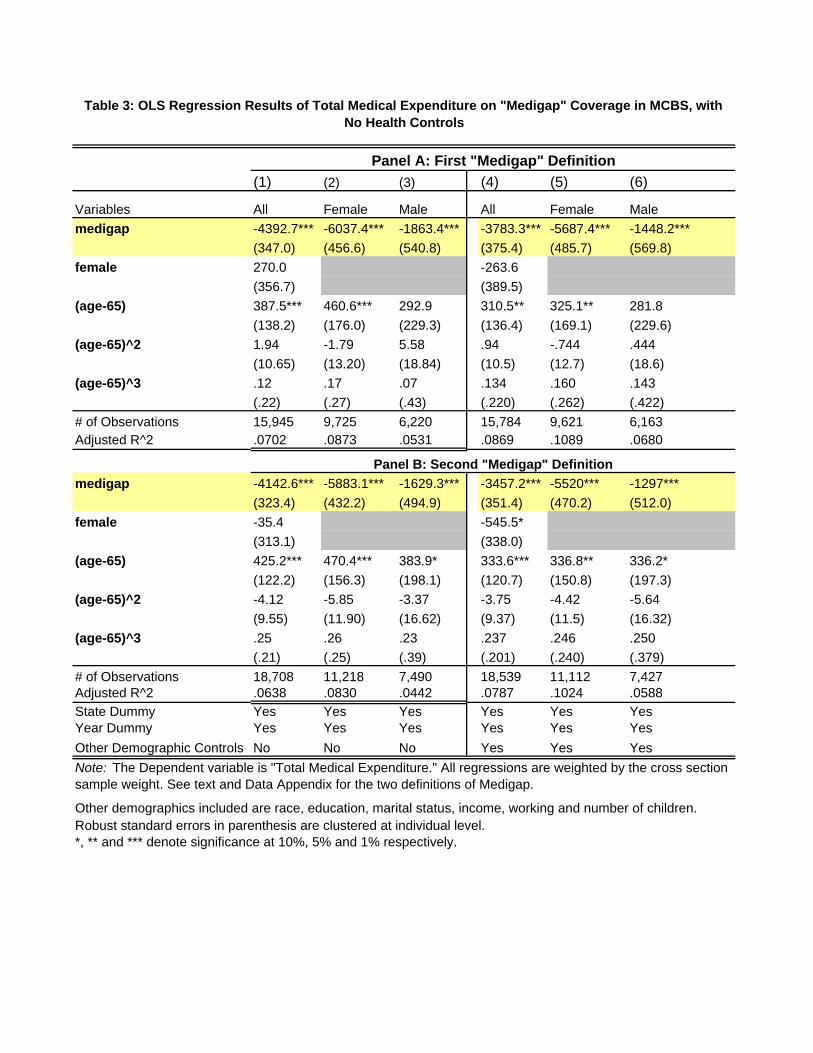
(1) (2) (3) (4) (5) (6)

Variables All Female Male All Female Male medigap -4392.7*** -6037.4*** -1863.4*** -3783.3*** -5687.4*** -1448.2***

(347.0) (456.6) (540.8) (375.4) (485.7) (569.8)female 270.0 -263.6

(356.7) (389.5)(age-65) 387.5*** 460.6*** 292.9 310.5** 325.1** 281.8

(138.2) (176.0) (229.3) (136.4) (169.1) (229.6)(age-65)^2 1.94 -1.79 5.58 .94 -.744 .444

(10.65) (13.20) (18.84) (10.5) (12.7) (18.6)(age-65)^3 .12 .17 .07 .134 .160 .143

(.22) (.27) (.43) (.220) (.262) (.422)# of Observations 15,945 9,725 6,220 15,784 9,621 6,163Adjusted R^2 .0702 .0873 .0531 .0869 .1089 .0680

medigap -4142.6*** -5883.1*** -1629.3*** -3457.2*** -5520*** -1297***(323.4) (432.2) (494.9) (351.4) (470.2) (512.0)

female -35.4 -545.5*(313.1) (338.0)

(age-65) 425.2*** 470.4*** 383.9* 333.6*** 336.8** 336.2*(122.2) (156.3) (198.1) (120.7) (150.8) (197.3)

(age-65)^2 -4.12 -5.85 -3.37 -3.75 -4.42 -5.64(9.55) (11.90) (16.62) (9.37) (11.5) (16.32)

(age-65)^3 .25 .26 .23 .237 .246 .250(.21) (.25) (.39) (.201) (.240) (.379)

# of Observations 18,708 11,218 7,490 18,539 11,112 7,427Adjusted R^2 .0638 .0830 .0442 .0787 .1024 .0588State Dummy Yes Yes Yes Yes Yes YesYear Dummy Yes Yes Yes Yes Yes YesOther Demographic Controls No No No Yes Yes Yes

Robust standard errors in parenthesis are clustered at individual level.*, ** and *** denote significance at 10%, 5% and 1% respectively.

Table 3: OLS Regression Results of Total Medical Expenditure on "Medigap" Coverage in MCBS, with No Health Controls

Other demographics included are race, education, marital status, income, working and number of children.

Panel A: First "Medigap" Definition

Panel B: Second "Medigap" Definition

Note: The Dependent variable is "Total Medical Expenditure." All regressions are weighted by the cross section sample weight. See text and Data Appendix for the two definitions of Medigap.

(1) (2) (3) (4) (5) (6)

Variables All Female Male All Female Male medigap 1937.0*** 1677.3*** 2420.9*** 1732.8*** 1426.2*** 2210.1***

(257.6) (349.0) (397.4) (272.4) (358.4) (418.9)female -751.6*** -754.1***

(283.7) (294.0)(age-65) 394.5*** 417.5*** 355.4* 419.6*** 444.2*** 392.1**

(117.4) (145.0) (197.6) (113.3) (137.4) (198.9)(age-65)^2 -27.5*** -32.0*** -22.8 -28.3*** -32.7*** -25.2

(9.3) (11.4) (16.3) (9.0) (11.1) (16.4)(age-65)^3 .474** .548** .466 .491** .562** .520

(.207) (.254) (.380) (.202) (.247) (.382)# of Observations 14,129 8,371 5,758 14,105 8,365 5,740Adjusted R^2 .2087 .1915 .2462 .2135 .2007 .2484

medigap 1967.3*** 1638.5*** 2529.7*** 1760.2*** 1372.5*** 2353.1***(238.7) (311.5) (377.4) (255.9) (330.0) (398.3)

female -926.1*** -911.9***(264.0) (275.7)

(age-65) 371.6*** 404.5*** 371.8** 384.3*** 417.5*** 392.6**(104.1) (129.2) (171.1) (101.8) (124.0) (172.0)

(age-65)^2 -25.6*** -30.2*** -24.8* -25.6*** -30.3*** -26.3*(8.3) (10.2) (14.1) (8.1) (9.9) (14.1)

(age-65)^3 .418*** .504** .479 .420** .506** .520(.185) (.227) (.330) (.182) (.222) (.331)

# of Observations 16,885 9,860 7,025 16,853 9,852 7,001Adjusted R^2 .2001 .1906 .2342 .2042 .1991 .2362State Dummy Yes Yes Yes Yes Yes YesYear Dummy Yes Yes Yes Yes Yes YesOther Demographic Controls No No No Yes Yes Yes

Robust standard errors in parenthesis are clustered at individual level.*, ** and *** denote significance at 10%, 5% and 1% respectively.

The variables included as direct health controls are detailed in Data Appendix. The other demographics included are race, education, marital status, income, working and number of children.

Table 4: OLS Regression Results of Total Medical Expenditure on "Medigap" Coverage in MCBS, with Direct Health Controls

Panel A: First "Medigap" Definition

Panel B: Second "Medigap" Definition

Note: The Dependent variable is "Total Medical Expenditure." All regressions are weighted by the cross section sample weight. See text and Data Appendix for the two definitions of Medigap.

(1) (2) (3) (4) (5) (6)Variables All Female Male All Female Male medigap 2083.3*** 1601.1*** 2775.5*** 1838.7*** 1347.5*** 2450.0***

(280.6) (353.8) (426.3) (293.0) (361.7) (453.5)female -1311.2*** -1274.4***

(271.5) (285.4)(age-65) 421.8*** 447.6*** 436.0** 433.5*** 467.8*** 451.6**

(118.7) (151.5) (194.2) (116.9) (144.2) (196.6)(age-65)^2 -28.7*** -32.6*** -27.3* -28.6*** -32.3*** -26.7*

(9.2) (11.9) (16.0) (9.1) (11.6) (16.2)(age-65)^3 .479** .534** .543 .481** .513** .520

(.205) (.261) (.375) (.201) (.255) (.381)Factor1 321.0 -410.7*** 1097.1* 324.9 -415.5*** 1094.5*

(498.0) (89.0) (658.7) (495.1) (90.3) (662.0)Factor2 4917.5*** 4902.2*** 4880.6*** 4928.9*** 4976.5*** 4855.9***

(268.3) (343.2) (368.4) (269.3) (349.4) (357.9)Factor3 -2979.4*** -2500.8*** -4048.4*** -3055.1*** -2449.8*** -4211.7***

(306.2) (300.7) (623.9) (308.0) (307.7) (605.5)Factor4 -652.1** -684.3* -1073.5 -746.3** -794.9** -1141.8

(311.1) (384.3) (911.2) (309.7) (381.2) (895.8)Factor5 75.8 436.4* -2278.9* 28.7* 459.3* -2294.7*

(305.0) (253.8) (1340.1) (309.8) (252.8) (1308.9)# of Observations 14,129 8,371 5,758 14,105 8,337 5,731Adjusted R^2 .1398 .1345 .1792 .1448 .1450 .1857

medigap 2154.5*** 1577.6*** 2944.7*** 1914.2*** 1312.0*** 2628.6***(256.7) (321.1) (412.7) (207.8) (338.0) (426.4)

female -1468.5*** -1435.7***(249.1) (261.3)

(age-65) 433.1*** 442.3*** 421.8*** 434.9*** 452.4*** 414.9***(105.0) (134.7) (168.2) (103.9) (129.6) (170.6)

(age-65)^2 -29.2*** -31.6*** -27.1** -28.5*** -31.1*** -25.2*(8.2) (10.6) (13.7) (8.1) (10.4) (13.8)

(age-65)^3 .468*** .508** .484 .461* .489** .437(.184) (.234) (.322) (.181) (.230) (.325)

Factor1 147.6 -843.9*** 847.2 144.3 -865.8*** 878.8(422.3) (88.3) (767.3) (420.1) (89.0) (808.3)

Factor2 4908.8*** 4743.5*** 4982.6*** 4918.5*** 4820.0*** 4970.3***(246.2) (310.0) (360.9) (247.6) (316.7) (356.9)

Factor3 -2949.4*** -2578.1*** -3560.8*** -3008.7*** -2537.1*** -3701.8***(265.3) (264.4) (515.9) (266.5) (269.2) (518.7)

Factor4 -435.3 -689.7** 181.3 -510.9* -771.5** 216.9(266.3) (333.7) (453.0) (265.8) (331.3) (458.2)

Factor5 182.9 408.2* -153.0 140.4 425.2* -184.0(267.5) (229.2) (409.4) (271.7) (227.9) (408.4)

# of Observations 16,885 9,860 7,025 16,853 9,822 6991Adjusted R^2 .1401 .1357 .1548 .1447 .1451 .1605State Dummy Yes Yes Yes Yes Yes YesYear Dummy Yes Yes Yes Yes Yes YesOther Demographic Controls No No No Yes Yes Yes

Robust standard error in parenthesis are clustered at individual level. *, ** and *** denote significance at 10%, 5% and 1% respectively.

The variables included as direct health controls are detailed in Data Appendix. The other demographics included are race, education, marital status, income, working and number of children.

Table 5: OLS Regression Results of Total Medical Expenditure on "Medigap" Coverage in MCBS, with Controls for Health Factors

Panel A: First "Medigap" Definition

Note: The Dependent variable is "Total Medical Expenditure." All regressions are weighted by the cross section sample weight. See text and Data Appendix for the two definitions of Medigap.

Panel B: Second "Medigap" Definition

EXP PCORR EXP PCORR EXP PCORR EXP PCORR EXP PCORR EXP PCORRFactor1 321.0 .0296 -410.7*** .0274 1097.1* .0342 147.6 .0269 -843.9*** .0373 847.2 .0267

(.000) (.012) (.009) (.000) (.000) (.025)Factor2 4917.5*** -.1166 4902.2*** -.1290 4880.6*** -.0978 4908.8*** -.1107 4743.5*** -.1193 4982.6*** -.0953

(.000) (.000) (.000) (.000) (.000) (.000)Factor3 -2979.4*** .0319 -2500.8*** .0425 -4048.4*** .0200 -2949.4*** .0297 -2578.1*** .0434 -3560.8*** .0138

(.000) (.000) (.129) (.000) (.000) (.247)Factor4 -652.1** -.0177 -684.3* -.0171 -1073.5 .0229 -435.3 -.0186 -689.7** -.0157 181.3 -.0389

(.035) (.117) (.083) (.016) (.120) (.001)Factor5 75.8 .0207 436.4* .0143 -2278.9* -.0204 182.9 .0333 408.2* .0258 -153.0 .0262

(.014) (.190) (.122) (.015) (.010) (.028)

# of Obs. 14,131 8,373 5,758 16,887 9,862 7,025

Note: The columns labelled with "EXP" are the regression coefficients from Table 3 for the specification with other demographic controls. They are included in the table for the interpretation of the factors.The columns labelled with "PORR" lists the partial correlation of "medigap" with the corresponding factors. The number in parenthesis is the significance level of the correlation.

All Female Male

Table 6: Partial Correlation between "Medigap" Coverage and Health Factors in MCBS, Conditional on Gender and Age

Panel A: First "Medigap" DefinitionMaleAll Female

Panel B: Second "Medigap" DefinitionFactors

All Female Male All Female Male All Female Male All Female Male

Female 0.602 1.000 .000 .572 1.000 .000 .593 1.000 .000 .558 1.000 .000(.489) (.000) (.000) (.495) (.000) (.000) (.491) (.000) (.000) (.497) (.000) (.000)

Age 75.808 76.546 74.690 75.301 75.847 74.415 75.602 76.336 74.534 75.112 75.672 74.263(7.729) (8.047) (7.076) (7.078) (7.353) (6.611) (7.612) (7.933) (6.983) (7.010) (7.295) (6.547)

Medigap .459 .462 .455 .486 .495 .473 .545 .540 .552 .568 .565 .573(.498) (.495) (.498) (.500) (.500) (.499) (.498) (.498) (.497) (.495) (.496) (.495)

Medicare_AB .958 .966 .945 .949 .947 .953 .955 .965 .940 .948 .947 .949(.201) (.181) (.228) (.219) (.223) (.213) (.208) (.185) (.237) (.223) (.224) (.220)

Black .091 .094 .087 .076 .082 .069 .087 .090 .082 .072 .078 .065(.288) (.293) (.282) (.265) (.274) (.253) (.281) (.286) (.275) (.259) (.269) (.246)

Hispanic .077 .073 .082 .042 .040 .046 .070 .067 .074 .039 .036 .042(.266) (.261) (.275) (.202) (.195) (.211) (.255) (.251) (.261) (.193) (.188) (.200)

Married .485 .344 .698 .532 .391 .743 .512 .371 .717 .543 .390 .755(.500) (.475) (.459) (.499) (.488) (.437) (.500) (.483) (.451) (.498) (.488) (.430)

Widowed .379 .523 .162 .350 .481 .151 .361 .504 .153 .342 .478 .146(.485) (.499) (.368) (.477) (.500) (.358) (.480) (.500) (.360) (.474) (.500) (.353)

Divorced .079 .084 .071 .079 .092 .063 .074 .079 .068 .077 .092 .060(.270) (.287) (.258) (.269) (.289) (.244) (.262) (.269) (.252) (.267) (.290) (.238)

# of children 2.998 2.912 3.127 3.193 3.134 3.283 2.978 2.890 3.106 3.163 3.093 3.263(2.238) (2.224) (2.252) (2.228) (2.227) (2.238) (2.187) (2.177) (2.194) (2.193) (2.198) (2.193)

Working .124 .088 .179 .137 .118 .165 .127 .091 .180 .137 .118 .163(.330) (.284) (.383) (.344) (.323) (.371) (.333) (.287) (.385) (.344) (.322) (.369)

Less than HS .343 .342 .345 .306 .306 .307 .323 .322 .323 .285 .287 .280(.377) (.375) (.384) (.360) (.362) (.361) (.368) (.367) (.368) (.348) (.350) (.347)

High School .276 .300 .240 .363 .387 .329 .276 .300 .240 .357 .382 .324(.447) (.458) (.427) (.481) (.487) (.470) (.447) (.458) (.427) (.479) (.486) (.468)

Some College .210 .217 .198 .177 .183 .169 .220 .227 .209 .179 .186 .170(.407) (.413) (.399) (.381) (.386) (.375) (.414) (.419) (.406) (.383) (.389) (.376)

College .081 .068 .101 .080 .065 .099 .088 .074 .108 .086 .070 .107(.273) (.252) (.301) (.271) (.247) (.299) (.283) (.261) (.310) (.281) (.255) (.309)

Note: Statistics are calculated using cross section sample weights. Standard deviations are in parenthesis. Number of observations vary by variable and sample.

Table 7: Descripitive Statistics of MCBS and HRS Samples

MCBS HRSPanel B: Second Definition of MedigapPanel A: First Definition of Medigap

MCBS HRS

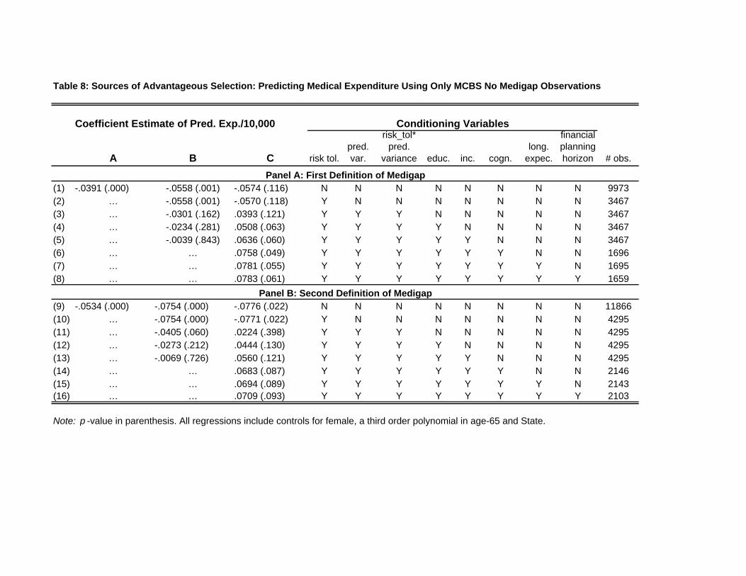
A B C risk tol.pred. var.

risk_tol* pred.

variance educ. inc. cogn.long.

expec.

financial planning horizon # obs.

(1) -.0391 (.000) -.0558 (.001) -.0574 (.116) N N N N N N N N 9973(2) … -.0558 (.001) -.0570 (.118) Y N N N N N N N 3467(3) … -.0301 (.162) .0393 (.121) Y Y Y N N N N N 3467(4) … -.0234 (.281) .0508 (.063) Y Y Y Y N N N N 3467(5) … -.0039 (.843) .0636 (.060) Y Y Y Y Y N N N 3467(6) … … .0758 (.049) Y Y Y Y Y Y N N 1696(7) … … .0781 (.055) Y Y Y Y Y Y Y N 1695(8) … … .0783 (.061) Y Y Y Y Y Y Y Y 1659

(9) -.0534 (.000) -.0754 (.000) -.0776 (.022) N N N N N N N N 11866(10) … -.0754 (.000) -.0771 (.022) Y N N N N N N N 4295(11) … -.0405 (.060) .0224 (.398) Y Y Y N N N N N 4295(12) … -.0273 (.212) .0444 (.130) Y Y Y Y N N N N 4295(13) … -.0069 (.726) .0560 (.121) Y Y Y Y Y N N N 4295(14) … … .0683 (.087) Y Y Y Y Y Y N N 2146(15) … … .0694 (.089) Y Y Y Y Y Y Y N 2143(16) … … .0709 (.093) Y Y Y Y Y Y Y Y 2103

Note: p -value in parenthesis. All regressions include controls for female, a third order polynomial in age-65 and State.

Panel B: Second Definition of Medigap

Panel A: First Definition of Medigap

Table 8: Sources of Advantageous Selection: Predicting Medical Expenditure Using Only MCBS No Medigap Observations

Conditioning VariablesCoefficient Estimate of Pred. Exp./10,000

A B Crisk tol.

pred. var.

risk_tol* pred.

variance educ. inc. cogn.long.

expec.

financial planning horizon # obs.

(1) -.0275 (.004) -.0519 (.002) -.0465 (.167) N N N N N N N N 9973(2) … -.0519 (.002) -.0461 (.169) Y N N N N N N N 3467(3) … -.0296 (.173) .0263 (.307) Y Y Y N N N N N 3467(4) … -.0222 (.313) .0380 (.133) Y Y Y Y N N N N 3467(5) … -.0034 (.862) .0490 (.091) Y Y Y Y Y N N N 3467(6) … … .0562 (.068) Y Y Y Y Y Y N N 1696(7) … … .0580 (.074) Y Y Y Y Y Y Y N 1695(8) … … .0587 (.080) Y Y Y Y Y Y Y Y 1659

(9) -.0429 (.000) -.0776 (.000) -.0832 (.005) N N N N N N N N 11866(10) … -.0777 (.000) -.0827 (.005) Y N N N N N N N 4295(11) … -.0026 (.956) -.0284 (.705) Y Y Y N N N N N 4295(12) … .0176 (.695) .0140 (.853) Y Y Y Y N N N N 4295(13) … .0490 (.262) .0483 (.518) Y Y Y Y Y N N N 4295(14) … … .0567 (.438) Y Y Y Y Y Y N N 2146(15) … … .0618 (.402) Y Y Y Y Y Y Y N 2143(16) … … .0695 (.346) Y Y Y Y Y Y Y Y 2103

Note: p-value in parenthesis. All regressions include controls for female, a third order polynomial in age-65 and State.

Panel B: Second Definition of Medigap

Table 9: Sources of Advantageous Selection: Predicting Medical Expenditure Using All Observations in MCBS

Conditioning Variables

Panel A: First Definition of Medigap

Coefficient Estimate of Pred. Exp./10,000

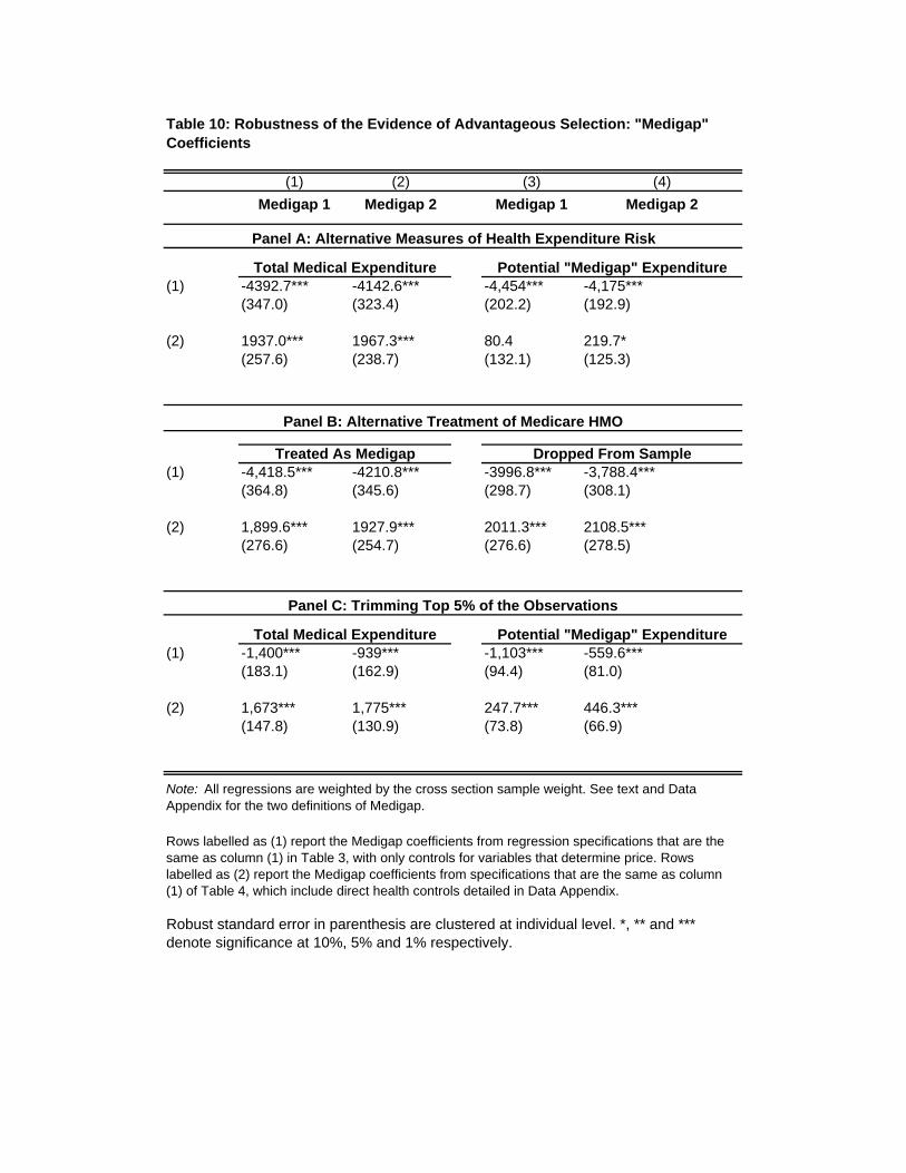
(1) (2) (3) (4)Medigap 1 Medigap 2 Medigap 1 Medigap 2

(1) -4392.7*** -4142.6*** -4,454*** -4,175***(347.0) (323.4) (202.2) (192.9)

(2) 1937.0*** 1967.3*** 80.4 219.7*(257.6) (238.7) (132.1) (125.3)

(1) -4,418.5*** -4210.8*** -3996.8*** -3,788.4***(364.8) (345.6) (298.7) (308.1)

(2) 1,899.6*** 1927.9*** 2011.3*** 2108.5***(276.6) (254.7) (276.6) (278.5)

(1) -1,400*** -939*** -1,103*** -559.6***(183.1) (162.9) (94.4) (81.0)

(2) 1,673*** 1,775*** 247.7*** 446.3***(147.8) (130.9) (73.8) (66.9)

Dropped From Sample

Total Medical Expenditure Potential "Medigap" Expenditure

Robust standard error in parenthesis are clustered at individual level. *, ** and *** denote significance at 10%, 5% and 1% respectively.

Note: All regressions are weighted by the cross section sample weight. See text and Data Appendix for the two definitions of Medigap.

Rows labelled as (1) report the Medigap coefficients from regression specifications that are the same as column (1) in Table 3, with only controls for variables that determine price. Rows labelled as (2) report the Medigap coefficients from specifications that are the same as column (1) of Table 4, which include direct health controls detailed in Data Appendix.

Table 10: Robustness of the Evidence of Advantageous Selection: "Medigap" Coefficients

Panel A: Alternative Measures of Health Expenditure Risk

Panel B: Alternative Treatment of Medicare HMO

Panel C: Trimming Top 5% of the Observations

Total Medical Expenditure Potential "Medigap" Expenditure

Treated As Medigap

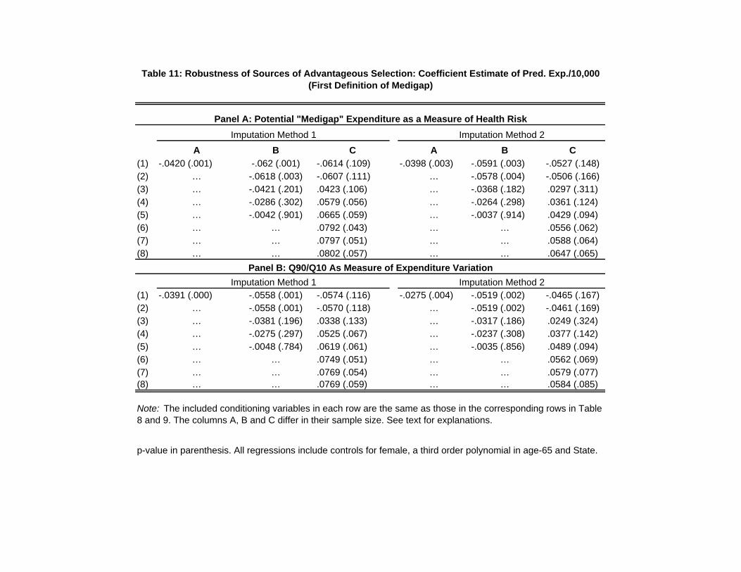
A B C A B C(1) -.0420 (.001) -.062 (.001) -.0614 (.109) -.0398 (.003) -.0591 (.003) -.0527 (.148)(2) … -.0618 (.003) -.0607 (.111) … -.0578 (.004) -.0506 (.166)(3) … -.0421 (.201) .0423 (.106) … -.0368 (.182) .0297 (.311)(4) … -.0286 (.302) .0579 (.056) … -.0264 (.298) .0361 (.124)(5) … -.0042 (.901) .0665 (.059) … -.0037 (.914) .0429 (.094)(6) … … .0792 (.043) … … .0556 (.062)(7) … … .0797 (.051) … … .0588 (.064)(8) … … .0802 (.057) … … .0647 (.065)

(1) -.0391 (.000) -.0558 (.001) -.0574 (.116) -.0275 (.004) -.0519 (.002) -.0465 (.167)(2) … -.0558 (.001) -.0570 (.118) … -.0519 (.002) -.0461 (.169)(3) … -.0381 (.196) .0338 (.133) … -.0317 (.186) .0249 (.324)(4) … -.0275 (.297) .0525 (.067) … -.0237 (.308) .0377 (.142)(5) … -.0048 (.784) .0619 (.061) … -.0035 (.856) .0489 (.094)(6) … … .0749 (.051) … … .0562 (.069)(7) … … .0769 (.054) … … .0579 (.077)(8) … … .0769 (.059) … … .0584 (.085)

Note: The included conditioning variables in each row are the same as those in the corresponding rows in Table 8 and 9. The columns A, B and C differ in their sample size. See text for explanations.

p-value in parenthesis. All regressions include controls for female, a third order polynomial in age-65 and State.

Imputation Method 1 Imputation Method 2

Panel B: Q90/Q10 As Measure of Expenditure Variation

Panel A: Potential "Medigap" Expenditure as a Measure of Health Risk

Table 11: Robustness of Sources of Advantageous Selection: Coefficient Estimate of Pred. Exp./10,000 (First Definition of Medigap)

Imputation Method 1 Imputation Method 2

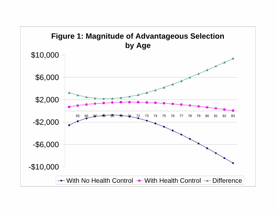
Figure 1: Magnitude of Advantageous Selection by Age

-$10,000

-$6,000

-$2,000

$2,000

$6,000

$10,000

65 66 67 68 69 70 71 72 73 74 75 76 77 78 79 80 81 82 83

With No Health Control With Health Control Difference

Category Variable DataHealth Total expendidure MCBS Total annual health care expenditure for 12 months of the survey year. Expenditure includes dataexpenditure from Medicare administrative files and survey responses for out-of-pocket and otherwise insured

expenditures.Insurance

medicare Indicators for whether the respondent is covered by medicare part A and part B.

medigap MCBS Indicator for whether repsondent, with medicare coverage also has self-purchased private healthinsurance. Those covered by employer provided health inurance, medicaid or VA Champus (Tri-care) are treated as missing.

HRS Indicator for whether respondent, with Medicare coverage also has private health insurance that issecondary to Medicare, and not purchased from a (spouse's) employer or union. Those covered by employer provided health inurance, medicaid or VA Champus (Tri-care) are treated as missing.

medigap2 Variable equal to one if medigap is equal to one, or if covered by employer sponsored healthinsurance and pay more than $500 per year in premiums.

Demographics race Indicators for self-reported black, other and non-response

hispanic Indicators for self-reported hispanic and non-response

education Indicators for highest grade completed less than 8th grade, some high school, high school graduate, some college, college graduate, at least some grad school and non-response

marital status Indicators for maried, widowed, divorced, separated and non-response

number of children The number of children the respondent has ever had.

income MCBS Indicators for self-reported total household income in $5,000 intervals from $5,000 to $50,000,and $50,000 plus

HRS Same indicators as above, except in this case we use reported as well as imputed values for totalhousehold income. Imputations are those generated by RAND. See http://hrsonline.isr.umich.edu/meta/rand/randhrse/randhrse.pdf for details of the imputation.

work status Indicators if currently working for pay and for non-response.

Description

DATA APPENDIX

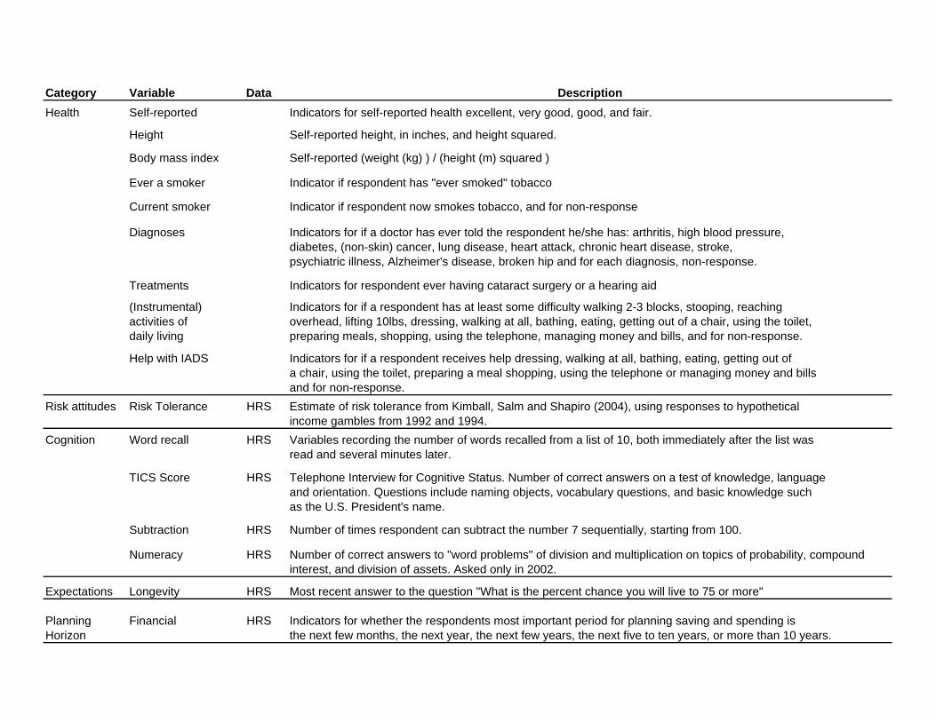
Category Variable DataHealth Self-reported Indicators for self-reported health excellent, very good, good, and fair.

Height Self-reported height, in inches, and height squared.

Body mass index Self-reported (weight (kg) ) / (height (m) squared )

Ever a smoker Indicator if respondent has "ever smoked" tobacco

Current smoker Indicator if respondent now smokes tobacco, and for non-response

Diagnoses Indicators for if a doctor has ever told the respondent he/she has: arthritis, high blood pressure, diabetes, (non-skin) cancer, lung disease, heart attack, chronic heart disease, stroke, psychiatric illness, Alzheimer's disease, broken hip and for each diagnosis, non-response.

Treatments Indicators for respondent ever having cataract surgery or a hearing aid

(Instrumental) Indicators for if a respondent has at least some difficulty walking 2-3 blocks, stooping, reachingactivities of overhead, lifting 10lbs, dressing, walking at all, bathing, eating, getting out of a chair, using the toilet,daily living preparing meals, shopping, using the telephone, managing money and bills, and for non-response.

Help with IADS Indicators for if a respondent receives help dressing, walking at all, bathing, eating, getting out of a chair, using the toilet, preparing a meal shopping, using the telephone or managing money and billsand for non-response.

Risk attitudes Risk Tolerance HRS Estimate of risk tolerance from Kimball, Salm and Shapiro (2004), using responses to hypotheticalincome gambles from 1992 and 1994.

Cognition Word recall HRS Variables recording the number of words recalled from a list of 10, both immediately after the list wasread and several minutes later.

TICS Score HRS Telephone Interview for Cognitive Status. Number of correct answers on a test of knowledge, languageand orientation. Questions include naming objects, vocabulary questions, and basic knowledge such as the U.S. President's name.

Subtraction HRS Number of times respondent can subtract the number 7 sequentially, starting from 100.

Numeracy HRS Number of correct answers to "word problems" of division and multiplication on topics of probability, compoundinterest, and division of assets. Asked only in 2002.

Expectations Longevity HRS Most recent answer to the question "What is the percent chance you will live to 75 or more"

Planning Financial HRS Indicators for whether the respondents most important period for planning saving and spending isHorizon the next few months, the next year, the next few years, the next five to ten years, or more than 10 years.

Description