Source-Receptor Relationships for Ozone and Fine ... · PDF fileSource-Receptor Relationships for Ozone and Fine Particulates in the Eastern United States ... portion of this paper

Source-Receptor Relationships for Ozone and Fine Particulates in the Eastern United States

Jhih-Shyang Shih, Alan J. Krupnick, Michelle S. Bergin and Armistead G. Russell

May 2004 • Discussion Paper 04–25

Resources for the Future 1616 P Street, NW Washington, D.C. 20036 Telephone: 202–328–5000 Fax: 202–939–3460 Internet: http://www.rff.org

© 2004 Resources for the Future. All rights reserved. No portion of this paper may be reproduced without permission ofthe authors.

Discussion papers are research materials circulated by their authors for purposes of information and discussion. They havenot necessarily undergone formal peer review or editorial treatment.


Jhih-Shyang Shih, Alan J. Krupnick, Michelle S. Bergin, and Armistead G. Russell

Abstract A key question in developing effective mitigation strategies for ozone and particulate matter is identifying which source regions contribute to concentrations in receptor regions. Using a direct approach with a regional, multiscale three-dimensional model, we derive multiple source-receptor matrices (S-Rs) to show inter- and intrastate impacts of emissions on both ozone and PM2.5 over the eastern United States. Our results show that local (in-state) emissions generally account for about 23% of both local ozone concentrations and PM2.5 concentrations, while neighboring states contribute much of the rest. The relative impact of each state on others varies dramatically between episodes. In reducing fine particulate concentrations, we find that reducing SO2 emissions can be 10 times as effective as reducing NOx emissions. SO2 reductions can lead to some increase in nitrates, but this is relatively small. NOx reductions, however, lead to both ozone reductions and some reduction in nitrate and sulfate particulate matter.

Keywords: source-receptor, ozone, particulate matter, sensitivity analysis, air quality simulation, National Ambient Air Quality Standards

JEL Classification Numbers: Q2, Q25

Contents

Introduction............................................................................................................................. 1

Modeling Approach ................................................................................................................ 3

Model Description .............................................................................................................. 3

Application Description ...................................................................................................... 4

Model Performance............................................................................................................. 5

Results and Discussion............................................................................................................ 7

Sensitivity Results............................................................................................................... 7

Derivation of Multiple Pollutant S-R Matrices................................................................... 7

Ozone Sensitivity and Control Effects................................................................................ 9

PM2.5 Sensitivity and Control Effects ............................................................................... 11

Comparison of Long-Range Response of Ozone and PM2.5 Sensitivities ........................ 13

Issues of Nonlinearity and Uncertainty............................................................................. 14

Conclusions............................................................................................................................ 14

References.............................................................................................................................. 16


Jhih-Shyang Shih, Alan J. Krupnick, Michelle Bergin, and Armistead G. Russell ∗

Introduction Controversy over the extent to which emissions in one state affect air quality in other states

has been a central feature of the debate over air pollution control policy since 1990. This

controversy culminated in a series of lawsuits brought by East Coast states against Midwestern

states, charging that the latter were making attainment of the National Ambient Air Quality

Standard for ozone much more difficult for the former. Additionally, given their influence in

creating fine particulate concentrations (PM2.5: particles with a diameter less than 2.5 microns),

the temporal and spatial contribution of sulfur dioxide (SO2) and oxides of nitrogen (NOx)

emissions and the effect of NOx emissions reductions on ozone must be understood if effective

air pollution policies are to be crafted.

Ozone and PM2.5 share common sources and formation routes in the atmosphere. Ozone, a

gas, is formed secondarily in the atmosphere by reactions between NOx and volatile organic

compounds (VOCs) in the presence of sunlight. Fine particulate matter is composed of many

different chemical species, including (but not limited to) ammonium sulfate, ammonium nitrate,

and organic and elemental carbon. Depending on the chemical composition, PM2.5 can be

directly emitted (e.g., from diesel vehicles, dust, and biomass burning) and/or formed

secondarily from reactions of sulfur dioxide, NOx, ammonia (NH3), and VOCs. Controls placed

∗ Jhih-Shyang Shih and Alan J. Krupnick are Fellow and Senior Fellow, respectively, at Resources for the Future. Michelle Bergin and Armistead G. Russell are Ph.D. candidate and professor, respectively, at Georgia Institute of Technology. We thank Yueh-Jiun Yang, Jim Wilkinson, Jim Boylan, Allen Basala, Sheau-Rong Lou, Dick Morgenstern and Kris Wernstedt for valuable discussions. We are grateful to Lisa Crooks and Mike Batz for research assistance. This study is partly supported by a partnership grant from the USEPA and NSF and through a USEPA STAR graduate fellowship. Note that superscripts refer to numbered references on pages 16–17.

1

Resources for the Future Shih, Krupnick, Bergin, and Russell

to reduce one form of particulate may affect concentrations of the other, though not necessarily

proportionally or even in the same direction. For example, reducing SO2 emissions will generally

lead to a reduction in sulfate particulate matter, though less than proportionally.1 Further, the

reduction in sulfate leads to more ammonia being available to form particulate ammonium

nitrate—i.e., there is a “rebound” in the amount of particulate formed. The two effects mitigate

the total PM reduction that might be first expected. Also investigated is the “bounce-back”

effect, where NOx reductions can lead to localized increases in ozone due to reduced scavenging

of ozone and ozone precursors. Typically, this happens within a few tens of kilometers of the

source region studied, with reductions found downwind.

Previous studies have explored the responses of ozone and of PM2.5 to various controls.2-5

Control strategies exist that lower both PM2.5 and ozone concurrently, or lower one or the other.

Thus, from an air quality management perspective, it is desirable to understand the relative

efficacy of NOx and SO2 emissions reductions in controlling these air pollutants.

To address these issues, we developed a new modeling approach to derive multiple source-

receptor sensitivity matrices (S-Rs). 6 Independence, additivity, and linearity are assumed, and

have been demonstrated to be reasonably accurate.1 We compare the relative effectiveness of

regional (interstate) vs. local (intrastate) controls on NOx, and SO2 emissions as they affect ozone

and PM2.5 concentrations, the effectiveness of controlling NOx from elevated sources (i.e.,

electric utilities and large industrial plants), the relative effectiveness of reducing NOx vs. SO2

emissions to reduce PM2.5, and the sensitivity of these results to different weather patterns. We

study two very different meteorological episodes (in July and May 1995), each lasting

approximately 10 days. The 20 days allow us to investigate the impact of meteorological

variability on pollutant transport and local production. We also investigate the extent of the

“bounce-back” effect and the “rebound” effect, reducing part of the expected benefit from

controls. Finally, we investigate to what degree the efficacy of controls depends on how one

quantifies the response—e.g., looking at a spatial (area) weighting or considering exposure by

using a population-based approach.

2


Modeling Approach

Model Description In this study, the Urban-to-Regional Multiscale (URM) One Atmosphere Model (URM-

1ATM)7-8 and the Regional Atmospheric Modeling System (RAMS) are used to account for the

processes significantly affecting ozone and PM2.5 concentrations in the atmosphere, including

atmospheric physics, gas and aerosol phase chemistry, cloud and precipitation processes, and wet

and dry deposition. RAMS is used to recreate the physics of an historical period of time,

providing details and spatial coverage unavailable from observations. URM-1ATM solves the

atmospheric diffusion equation (ADE) for the change in concentration, c, of species i with time,

( ) ( ) iiiii Sfcctc

++∇•∇=•∇+∂∂ Ku (1)

where u is a velocity field, K is the diffusivity tensor, fi represents the production by chemical

reaction of species i, and Si represents sources and sinks of species i. As used here, a direct

sensitivity capability using the Direct Decoupled Method in Three Dimensions (DDM-3D)1-2 is

employed to calculate the local sensitivities of specified model outputs simultaneously with

concentrations. As shown in Equation 2, the sensitivity, Sij, of a model output, Ci (such as

pollutant concentration of species i) to specified model inputs or parameters, Pj (e.g., elevated

NOx emissions) is calculated as the ratio of the change in output Ci to an incremental change of

input or parameter Pj.

j

iij P

CS∂∂

= (2)

This leads to an additional set of equations that are solved concurrently with the

concentrations, but the structure of those equations is very similar to the original (Equation 1),

and is solved efficiently. This sensitivity is a local derivative, so a linear assumption is then made

to extrapolate the result to a non-zero perturbation. This assumption has been well tested for the

3


variables of interest for this study.1 A more detailed description of the model is available

elsewhere.8-9

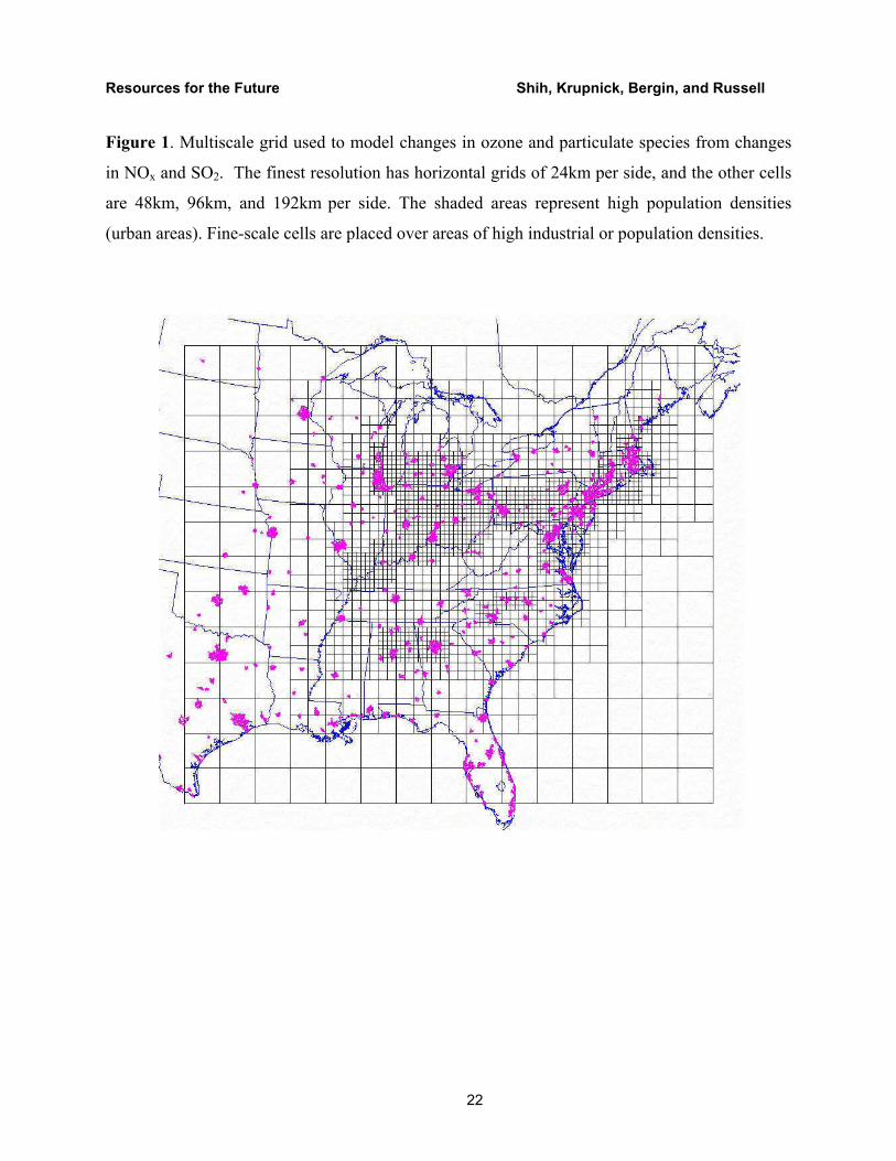
Application Description We use a multiscale grid structure encompassing the eastern United States (Figure 1). The

finest grids are placed over major source regions such as the Ohio River Valley, where many

power plants and large industries are located, and over highly populated regions such as the East

Coast corridor. This approach allows evaluation of potential population exposure to pollutants

and captures high-population-related sources such as automobile exhaust, fast food restaurants,

and so forth. Here, the term “potential exposure” denotes that we do not take into account micro-

environmental variations in concentrations or variations in individual activities. The vertical grid

has seven nonuniform layers, with the thinnest layer near the ground and the layers thickening

with an increase in altitude. This vertical scheme allows detailed treatment of ground-level

sources and best represents ground-level mixing and dry deposition processes, allowing for

diurnal changes in mixing depths, and capturing aloft multiday transport events. A comparison of

the effects of different grid scales and spatial allocation on model performance is presented

elsewhere.10

URM-1ATM is applied to two well-studied episodes occurring in July 9-19, 1995 and May

22-29, 1995. These base episodes were selected because high-quality and complete data was

available, was previously modeled using a different multiscale grid definition but with the same

simulation system,8 and because the data covered large meteorological variation with moderate

to high pollution formation. Meteorological information is developed using the Regional

Atmospheric Modeling System (RAMS)11 in a nonhydrostatic mode, including cloud and rain

microphysics. Prevailing winds in these episodes are toward the East Coast from the Midwest in

July, and toward the Southeast from the Mid-southern states in May. These are common wind

patterns for the summer and spring seasons, respectively.

4


Emissions were generated using the Emissions Modeling System (EMS-95).12 Because

1995 emissions are not relevant for future policy evaluation, 2010 day-specific emissions are

estimated under conditions that are anticipated with changes in population growth, vehicle

turnover, emissions control technologies, and anticipated emissions regulations. These future

scenarios are used to evaluate potential control strategies. Meteorological and initial and

boundary conditions are hourly and day-specific, and are held constant for base and future years.

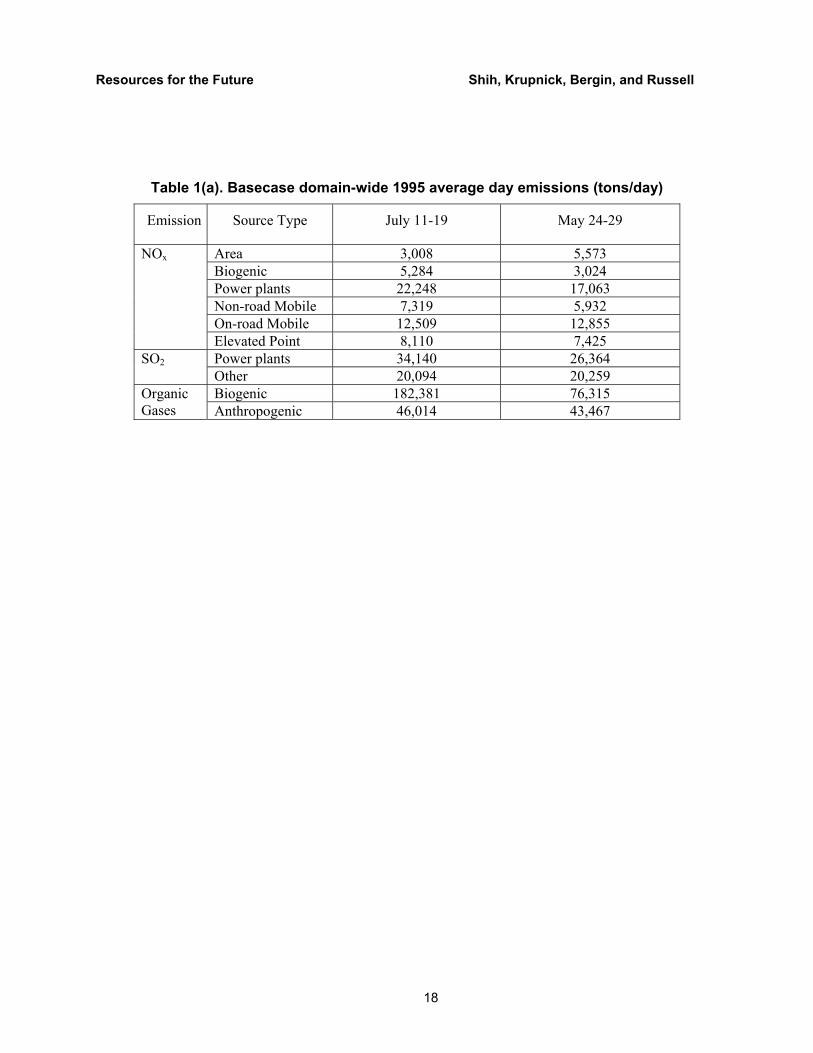
Table 1a presents the estimated average day emissions for the 1995 basecases and the state-

specific average day 2010 (future case) emissions. The emissions differences between 1995

basecases and the 2010 future case are due to implementation of the Tier 2 automotive emissions

regulations, the “NOx SIP Call,” acid deposition controls from the 1990 Clean Air Act

Amendments (CAAA), and other controls. Additional information on these model inputs is

described elsewhere.8-9

Model Performance Both of the 1995 basecase episodes have been used to evaluate model performance against

ambient measurements. Excluding model ramp-up days, nine and six days of simulation are

available for evaluation in the July and May episodes, respectively. Data from the U.S.

Environmental Protection Agency’s Aerometric Information Retrieval System (AIRS)13 is used

to evaluate model performance for ozone prediction. EPA guidelines for urban scale ozone

modeling are +/- 15% for Normalized Mean Bias (NMB), and +/- 35% for Normalized Mean

Error (NME). This regional-scale application resulted in an average NMB for ozone of 3.2% for

the May episode and of 1.6% for the July episode; the NME was 16.8% for May and 21.4% for

July. All these results were well within the stated guidelines. These values are calculated from

measurements at sites coinciding with either 24km2 or 48km2 cells. Data was available from

nearly 500 sites for each episode.

The Interagency Monitoring of Protected Visual Environments (IMPROVE) network14

provides 24-hour averaged speciated aerosol data taken on Wednesday and Saturday of each

week in our episodes, and this data is used to evaluate model performance for aerosols. Three

5


days of data was available during the July episode (July 12, 15, and 19), with measurements

from 18 sites in total, 12 of which coincided with 24km2 or 48km2 cells. These sites resulted in

an average NMB for PM2.5 of -24.6% and an average NME of 31.67%. Two days of data was

available for the May episode (May 24 and 27), with measurements from 17 sites in total, 11 of

which coincided with 24km2 or 48km2 cells. These sites resulted in an average NMB for PM2.5 of

-9.4% and an average NME of 28.30%. There are no current guidelines to indicate acceptable

model performance for aerosols. A detailed description of ozone and speciated aerosol model

performance for this application is presented elsewhere.10

Figures 2a and 3a show sample results for 2010 ozone and PM2.5 concentrations for the

July episode. The predicted one-hour daily maximum ozone concentrations for the entire domain

for the July episode are between 84.5 ppb and 104 ppb, well below the peak levels simulated

using the 1995 emissions (which is 120 ppb), showing the impact of predicted future controls.

The ozone concentration reaches its peak on the fourth day of the episode. The predicted 24-hour

average daily maximum PM2.5 concentrations over the entire domain for the July episode are

mostly between 46.7µg/m3 and 70 µg/m3. The concentrations start exceeding 59 µg/m3 after the

third day, peak on July 14, and decrease again after July 15.

May’s lower temperature than July explains its lower ozone and PM2.5 concentrations. The

ozone concentration for the May episode is between 61.6 ppb and 89.5 ppb, about 20% lower, on

average, than the concentration during the July episode. The 24-hour average PM2.5

concentration during the May episode is between 25.4 µg/m3 and 65.5 µg/m3, about 22% lower

than the concentration during the July episode.

6


Results and Discussion

Sensitivity Results After ensuring adequate model performance and developing future case simulations, the

2010 episodes are used to examine the sensitivity and control effects of ozone and aerosol

concentrations to reductions in specific emissions source types in different states. Here, S-R

coefficients are derived based on 30% emissions reductions. Nineteen states (or state

combinations) are evaluated as both sources and receptors. Results from reductions in two major

source types are presented: elevated NOx, such as from power plants and large industrial sites;

and total SO2 emissions, largely elevated emissions from coal-fired power plants. As examples,

Figures 2b and 3b show the “sensitivity” of ozone and PM2.5, respectively, resulting from

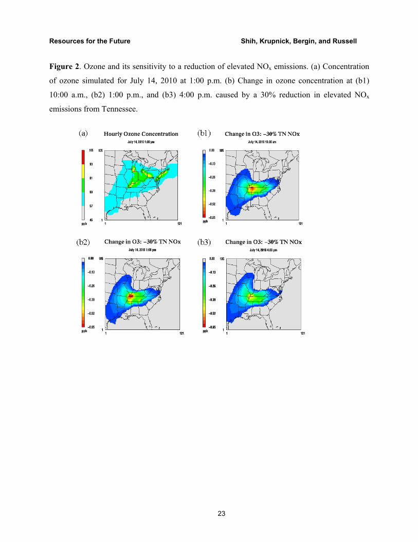
emissions reductions in Tennessee during the July 2010 episode. Figures 2b(1-3) show the

change in concentration of one-hour daily maximum ozone plumes at three different times of the

day when elevated NOx emissions are reduced by 30%. The impact on ozone concentrations in

other states is obvious (Figures 2b1 and 2b3). As is discussed later, some states, particularly

those near the Atlantic coast, are clearly receptors of many states’ emissions during the episodes

simulated (Figures 4-5).

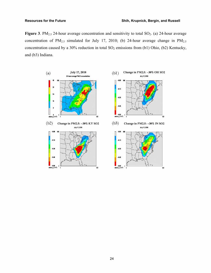
Figure 3a shows the baseline results for PM2.5 concentrations during July 17, 2010, and

Figures 3b(1-3) show PM2.5 sensitivity to 30% SO2 emissions reductions from OH, KY, and IN.

The results clearly show the interstate impact of emissions reductions from these states.

Derivation of Multiple Pollutant S-R Matrices The receptor states/regions of interest typically cover multiple simulation grid cells.

Therefore, to derive source-receptor matrices (S-Rs), we aggregated individual grid cell

sensitivity values to a single receptor site value. These sensitivity values represent the marginal

reduction of emissions from the source region to ozone or PM2.5 reduction at a receptor site. The

sensitivity used for aggregation is the change of pollutant concentration at the peak of the

specified time scale (one-hour or eight-hour daily maximum for ozone, and 24-hour average for

7


PM2.5). This source-receptor aggregation is performed on both a population-weighted and an

area-weighted basis. Population-weighted S-Rs are needed for estimating potential health

benefits from application of source controls, and also give a better proxy for health effects than

do area-weighted measures. From a regulatory perspective, the population-weighted S-Rs are

also more useful because they better apply to the urban areas (of course, under the Clean Air Act,

people living in rural areas are accorded the same level of protection as people in urban areas.)

The area-weighted S-Rs are useful to see the pure spatial and temporal effects of emissions on

concentrations.

Over the number of episode days, D, for the number of grid cells, i, covering receptor site

r, 1HDMsr is the area- or population-weighted one-hour daily maximum ozone source receptor

coefficient in change of ppb at receptor r per 1,000 tons/day of NOx emissions reduction from

source s.

[ ]1000*

**

31

1

1 1

∑

∑∑

=

= =

∆

∆= I

iis

I

i

D

diid

sr

pDE

pOHDM (3)

Here, is the daily maximum one-hour ozone concentration change in cell i and day d. The

daily average is calculated for each grid cell. For population weighting, this value is multiplied

by the cell population (pi) and divided by the total population, or pi is set to 1 for area weighting.

The value is then divided by the source precursor’s average daily emissions reduction in tons per

day, (∆ ). This value is multiplied by 1,000 to convert it to ppb per 1,000 tons/day reduction.

This large factor is used for normalizing the sensitivities to avoid errors from very small

numbers.

3O id∆

Es

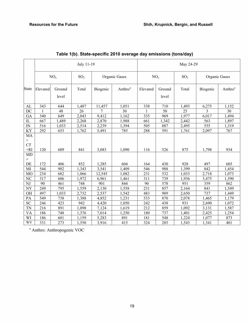
While a per ton sensitivity comparison is useful for evaluating equivalent emissions

reductions between states, states have very large differences in what they emit (see Table 1b),

and therefore in how much they are able to reduce emissions. To account for this discrepancy,

we also define and present what we term “control effects” to quantify the pollution reduction in

receptor states that would be achieved by reducing emissions from the 19 states/regions

8


combined. Control effects are calculated by multiplying the sensitivity matrix by a vector of 30%

emissions reductions from each of the source states. We use population-weighted sensitivities in

these control effects calculations.

Ozone Sensitivity and Control Effects There are four types of results combining the May and July episodes with area-weighted

and population-weighted sensitivities and control effects. We start with the July episode and

area-weighted sensitivities, and then compare these effects to those for May.

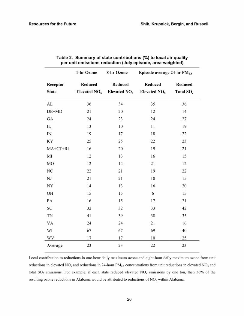
July Sensitivities. For the July episode and area-weighted S-Rs, states generally have only a

limited ability to reduce their own ozone concentrations by reducing elevated NOx emissions

(Table 2), although their own share of ozone reductions per unit NOx reduction is the single

largest for 53% of states (Figure 4). Results show that the average contribution of elevated NOx

control to local one-hour ozone concentrations is about 23%. The range of local control

contribution for elevated NOx is between 12% (MO) and 67% (WI). Note that emissions from

states outside of the 19 evaluated for sensitivities are not considered, and hence are not

contributing to this analysis. For this reason, a state such as Wisconsin may appear to be

contributing more to its own pollution than it actually is. The top five states contributing to

ozone concentrations in their own and other states (on a per unit emissions basis) are TN, KY,

VA, WV, and NC. The aggregate contributions to ozone per unit NOx reductions from these five

states to the rest of the domain are 12.4%, 8.7%, 8.5%, 7.3%, and 6.3%, respectively. In general,

downwind states (given our July conditions), such as MACTRI (MA, CT, and RI, combined),

MI, NY, MO, and NJ, contribute less to other states’ pollution.

We also calculate the sensitivities of eight-hour daily maximum ozone concentrations

consistent with the new U.S. ozone standard. The new standard is based on the fourth highest

eight-hour running average concentration of ozone in a year, while the historical standard is

based on the one-hour daily maximum. In general, the sensitivities of eight-hour daily maximum

9


ozone concentrations to NOx changes are slightly smaller than those for the one-hour daily

maximum ozone concentrations—2.5% smaller on average for elevated source NOx reductions.

To calculate health benefits obtained from emissions reductions, one would need to know

the change in population exposure. Since population is not uniformly distributed within

individual receptor state/regions, population-weighted sensitivities should be used in such

calculations instead of area-weighted sensitivities. For July, our population-weighted one-hour

NOx to ozone sensitivities are about 17.7% larger on average than area-weighted sensitivities,

with more than 74% of the local population-weighted sensitivities exceeding the corresponding

area-weighted sensitivities. Some of the differences can be quite striking. For example, for the

NJ receptor site, the one-hour ozone population-weighted sensitivity for NJ elevated NOx is

almost 40% bigger than that of its area-weighted counterpart (4.7 ppb vs. 3.5 ppb).

July Control Effects. Because the sensitivities were calculated based on a 30% reduction in

emissions, we estimate control effects for this same percentage change. This change, while

substantial, is lower than reductions proposed by the EPA Interstate Air Quality Rule, which

imply reductions in NOx and SO2 around 75% by 2015, on top of planned reductions already in

our 2010 baseline.

We find that the aggregate maximum one-hour ozone reduction ranges from 0.18 ppb (WI)

to 1.54 ppb (DE+MD) when elevated source emissions are reduced. These reductions may be

compared to baseline estimated ozone concentrations of 67.3 ppb (WI) and 77.2 ppb (DE+MD).

These reductions appear to be a small fraction of baseline ozone concentrations, in part because

emissions outside of the 19 states (other states and the domain boundaries) are not reduced,

contributing to elevated ozone levels.

July vs. May. Lower May temperatures and other differences in meteorological conditions

between May and July should result in lower predicted ozone concentrations in May, lower

ozone sensitivities to NOx in May, and different distributions of ozone contributions across states

(as seen in Figure 3). Indeed, the spatial and temporal average predicted one-hour daily

maximum ozone concentration in May is 53.9 ppb, while in July the average is 61.7 ppb. Also,

10


the average area-weighted one-hour daily maximum ozone sensitivity with respect to unit point

source NOx reductions for all sources and receptors for the May episode is 0.39 ppb, while it is

0.53 ppb for July, about 36% larger.

Less predictably, the local ozone sensitivity to elevated NOx reductions is higher for the

May episode (26% vs. 23% for July, on average). This implies that local control is more

effective in May compared to July. Because the winds come predominantly from the South in

May and from the Midwest in July, the top contributing states to other states’ ozone (as

measured by ozone sensitivities) tend to be from the South in May versus the Midwest in July

(Figure 3). It can also be seen that the variation among states’ contributions is larger in May.

PM2.5 Sensitivity and Control Effects

Fine particulate matter (considered here to be PM2.5) contains a mix of primary and

secondary components. In this paper, our discussion focuses on the sensitivity and control effects

of 24-hour averages of secondary PM2.5 only, starting with the July area-weighted sensitivities

with respect to sulfur dioxide and elevated source NOx emissions. The choice of a 24-hour

concentration averaging period is largely driven by the availability of measured data that was

available for model evaluation, and by the U.S. air quality standard, which is based on 24-hour

and one-year averages.

July Sensitivities. PM2.5 area-weighted sensitivities with respect to SO2 are far greater than those

with respect to NOx. For all sources and receptors during the July episode, the PM2.5 average

sensitivity with respect to total SO2 emissions is about 10 times the sensitivity with respect to

elevated point NOx. This is calculated from the average of the elemental ratio of two source-

receptor matrices, namely the PM2.5 source-receptor matrix with respect to total SO2 emissions

divided by the PM2.5 source-receptor matrix with respect to elevated point NOx. As a specific

example, OH contributes 0.57 µg/m3 of PM2.5 to PA per 1,000 tons of SO2 emissions (on

average), but NOx emissions from OH elevated point sources contribute only 0.047 µg/m3 to PA

11


(per 1,000 tons). Thus, reducing a ton of total SO2 emissions in OH will have about 12 times the

impact on PM2.5 concentrations in PA as would reducing a ton of OH point NOx emissions.

As expected, we found that decreasing SO2 always decreases sulfates and increases

nitrates, with the former change being about 28 times the latter for the July episode. Our PM2.5

sensitivities represent the net effect of SO2 emissions control (including sulfate aerosol reduction

and slight nitrate aerosol increases). West et al.15 studied marginal PM2.5 under an equilibrium

model to estimate the conditions for nonlinear response to changes in sulfate concentrations.

Their study considered local effects (without pollutant transport). They found that reductions in

SO2 emissions may cause an increase in aerosol nitrate (the “bounce-back” effect) because nitric

acid converts to nitrate. Such conditions are found to be common and significant in winter—

perhaps three to four times as prevalent as in summer. As West et al.15 pointed out, the bounce-

back effect can be so large that PM2.5 concentrations can actually increase. In our study (as in

others),8 we found that reducing SO2 emissions reduces PM2.5 concentrations, and that the

bounce-back effect is small. Consideration of winter periods might find a larger formation of

nitrate aerosol.

July Control Effects. By reducing elevated NOx emissions 30% from each of the 19 evaluated

states/regions, the aggregate PM2.5 reduction in these states ranges from 0.006 µg/m3 (MO) to

0.071 µg/m3 (KY), and are derived from small reductions in particulate nitrate, sulfate, and

ammonium. These reductions are small largely because nitrate levels during the summer in this

region are small. SO2 sensitivities are much larger. By reducing total SO2 emissions 30% from

each of these states, the aggregate reduction ranges from 0.13 µg/m3 (WI) to 2.55µg/m3 (VA).

The reduction contributed by source states is not equally distributed, depending on the emissions

reduction and S-R coefficients between sources and receptor states. Virtually all of the reduction

is due to decreases in sulfate and ammonium, and there is usually a concurrent increase in nitrate.

These results may be compared to the annual PM2.5 standard of 15 µg/m3 and the daily standard

of 65 µg/m3 (the average over three consecutive years of the 98th percentile of the daily value of

PM2.5). Also, note that states such as WI and MO are on the upwind side of the region being

12


studied, so are affected by emissions not accounted for in this analysis. For the July episode, our

24-hour daily average PM2.5 concentrations range from 4.7 µg/m3 to 32.7 µg/m3.

July versus May. We find that predicted PM2.5 concentrations in May are low, averaging 12.0

µg/m3, while in July they average 16.5 µg/m3. Also, the average 24-hour area-weighted PM2.5

sensitivities with respect to SO2 reductions for all sources and receptors for the May episode are

about one-fifth the average for July: 0.032 µg/m3 versus 0.17 µg/m3. This is because, compared

to the July episode, the May episode had faster winds, lower temperatures, more rain, and lower

concentrations of biogenic VOCs and hydroxyl radicals.

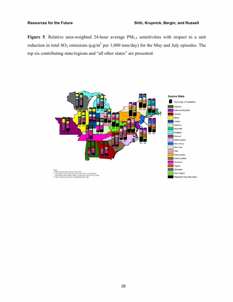
On the other hand, the fraction of local contributions to PM2.5 reductions is higher for the

May episode (29.0% vs. 23%, on average). In addition, because the winds come predominantly

from the South in May and from the Midwest in July, the top contributing states to other states’

PM2.5 tend to be from the South in May versus the Midwest in July. As with ozone, the variation

among states’ contributions is larger in May (Figure 5).

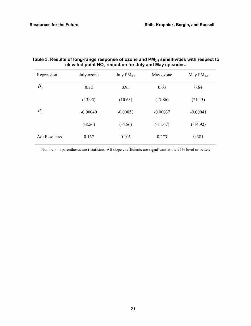
Comparison of Long-Range Response of Ozone and PM2.5 Sensitivities In this section, we examine how distance affects ozone and PM2.5 sensitivities. A

regression analysis was performed to explain ozone and PM2.5 sensitivities in terms of distance

from the source-state centroid to the receptor-state centroid. The dependent variable, , is the

remote sensitivity normalized by the source-state local sensitivity.

ijr

εββ ++= dr ijij *10 (4)

The right hand side, d , is the distance between the ith source-state centroid and the jth

receptor-state centroid.

ij

0β is the constant term of the regression equation. The slope ( 1β ) of this

simple regression model can be interpreted as the decreasing sensitivity per unit of distance. ε is

the stochastic error term. On average for the July episode, the PM2.5 sensitivity to elevated source

NOx emissions reductions is significant, decreasing about 0.053% per km; the ozone sensitivity

decreases about 0.040 % per km. For the May episode, the PM2.5 sensitivity reduction is 0.041%

13


per km and the ozone sensitivity reduction is about 0.037 % per km. Results of this regression

are shown in Table 3.

Issues of Nonlinearity and Uncertainty There are a number of important caveats that apply to the results of this study. First, we

assume that linearity holds within the 30% range of emissions changes and note that this

assumption was tested and found to be acceptable.1,6 Nevertheless, if the control measures were

to lead to emissions reductions much larger than 30%, the assumed linearity of response to

controls may no longer be satisfactory. In such a case, a second calculation at or near the reduced

emissions level may be necessary to account for the nonlinearity in pollutant response. Second,

we did not consider other sources of uncertainty and variability. For example, we only

considered two meteorological episodes (a total of 15 simulation days for use), and did not

extensively study the effect of meteorological input variation. While we have captured a high

and moderate pollutant episode, variation in wind direction, temperature, and other parameters

may significantly affect sensitivity results.

Conclusions While the absolute effects of NOx and SO2 control on ozone and PM2.5 concentrations are

sensitive to meteorological conditions, reducing elevated NOx emissions from our 19-state study

area by 30% from 2010 levels will have, at most, a modest impact on ozone concentrations and

PM2.5 concentrations in most of those states. Note, however, that boundary emissions and

emissions from other states in the domain were not eliminated. Comparatively, reducing SO2

emissions can have significant effects on PM2.5 concentrations. While “rebound” and “bounce-

back” effects are observed, they are generally not significant enough to result in perverse effects

on ozone during these episodes. The rebound effect on PM2.5 of SO2 reductions is generally small

(in terms of nitrate increases).

14


Long-range transport of precursors is an important issue for both pollutants, although

perhaps less so than is commonly thought. Local contributions to air pollution problems account

for about 23% of total ozone concentrations and PM2.5 concentrations, and neighbouring states

contribute much of the rest. The ozone sensitivity results are comparable with others in the

literature based on simpler models.16-18 The PM sensitivity coefficients, however, are smaller.18

This result may be due, in part, to the episodes chosen for study.

Area and population-weighted sensitivity matrices tell very different stories. We found that

population-weighted sensitivities exceed area-weighted sensitivities by as much as six times in

some regions. When evaluating health damages, one should use population-weighted sensitivities

to account for human exposure.

15


References 1. Odman, M.T., J.W. Boylan, J.G. Wilkinson, and A.G.Russell. Integrated Modeling for

Air Quality Assessment: The Southern Appalachian Mountains Initiative Project. J. Phys.

IV. 2002, 12 (PR10): 211-234

2. Russell, A.G., K.F. McCue, and G.R. Cass. Mathematical Modeling of the Formation of

Nitrogen-Containing Pollutants—2. Evaluation of the Effects of Emission Controls.

Environ. Sci. Technol. 1998, 22, 1336-1347.

3. Russell, A.G., K.F. McCue, and G.R. Cass. Mathematical Modeling of the Formation of

Nitrogen-Containing Air Pollutants—1. Evaluation of an Eulerian Photochemical Model.

Environ. Sci. Technol. 1998, 22, 263-271.

4. Meng, Z., D. Dabdub, and J.H. Seinfeld. Chemical Coupling Between Atmospheric

Ozone and Particulate Matter. Science 1997, 277 (5322), 116-119.

5. Stockwell, W.R., J.B. Milford, G.J. McRae, P. Middleton, and J.S. Chang. Nonlinear

Coupling in the NOx-SOx-Reactive Organic System. Atmos. Environ. 1988, 22, 2481-

2490.

6. Yang, Y.J., J.W. Wilkinson, and A.G. Russell. Fast, Direct Sensitivity Analysis of

Multidimensional Photochemical Models. Environ. Sci. Technol. 1997, 31, 2859-2868.

7. Kumar, N., M.T. Odman, and A.G. Russell. Multiscale Air Quality Modeling:

Application to Southern California. J. Geophys. Res. 1994, 99, 5385-5397.

8. Boylan, J.W., M.T. Odman, J.G. Wilkinson, A.G. Russell, K. Doty, W. Norris, and R.

McNider. Development of a Comprehensive, Multiscale “One Atmosphere” Modeling

System: Application to the Southern Appalachian Mountains. Atmos. Environ. 2002, 36,

3721-3734.

9. Bergin, M.S, J-S Shih, J.W. Boylan, J.G. Wilkinson, A.J. Krupnick, and A.G. Russell.

Inter- and Intra-State Impacts of NOx and SO2 Emissions on Ozone and Fine Particulate

Matter. To be submitted to Environ. Sci. Technol (2004).

16


10. Bergin, M.S, J.W. Boylan, J.G. Wilkinson, J-S Shih, A.J. Krupnick, and A.G. Russell.

Effects of Multiscale Grid Resolution and Spatial Distribution on 3D Model Performance

for Ozone and Aerosols. To be submitted to Environ. Sci. Technol (2004).

11. Pielke, R.A., W.R. Cotton, R.L. Walko, C.J. Tremback, W.A. Lyons, L.D. Grasso, M.E.

Nicholls, M.D. Moran, D.A. Wesley, T.J .Lee, and J. H. Copeland, A Comprehensive

Meteorological Modeling System - RAMS. Meteor. Atmos. Phys. 1992, 49, 69-91.

12. Wilkinson, J.G., C.F. Loomis, D.E. McNally, R.A. Emigh, and T.W. Tesche. Technical

Formulation Document: SARMAP/LMOS Emissions Modeling System (EMS-95). AG-

90/TS26 & AG-90/TS27. Alpine Geophysics, Pittsburgh, PA (1994).

13. USEPA EPA AIRS Data. U.S. Environmental Protection Agency, Office of Air Quality

Planning & Standards, Information Transfer & Program Integration Division,

Information Transfer Group. www.epa.gov/airsdata (2001).

14. NPS. National Park Service, Air Quality Research Division, Fort Collins. Anonymous ftp

at ftp://alta_vista.cira.colostate.edu in /data/improve (2000).

15. West, J.J., A.S. Ansari, and N.P. Spyros. Marginal PM2.5: Nonlinear Aerosol Mass

Response to Sulfate Reductions in the Eastern United States. J. Air & Waste Manage.

Assoc. 1999, 49, 1415-1424.

16. Rao, S.T.; Mount, T.D.; Dorris, G. Least Cost Control Strategies to Reduce Ozone in the

Northeastern Urban Corridor. The NY State Department of Environmental Conservation,

Division of Air Resources, Albany, NY (1999).

17. Krupnick, Alan J., Virginia D. McConnell, David H. Austin, Matthew Cannon, Terrell

Stoessell, and Brian Morton. The Chesapeake Bay and the Control of NOx Emissions: A

Policy Analysis, RFF discussion paper 98-46, August, Washington, DC. (1998).

18. Krupnick, A., V. McConnell, M. Cannon, T. Stoessell, and M. Batz. Cost-Effective NOx

Control in the Eastern United States, RFF discussion paper 00-18, August, Washington,

DC. (2000).

17

http://www.epa.gov/airsdata

ftp://alta_vista.cira.colostate.edu/


Table 1(a). Basecase domain-wide 1995 average day emissions (tons/day)

Emission Source Type July 11-19 May 24-29

Area 3,008 5,573 Biogenic 5,284 3,024 Power plants 22,248 17,063 Non-road Mobile 7,319 5,932 On-road Mobile 12,509 12,855

NOx

Elevated Point 8,110 7,425 Power plants 34,140 26,364 SO2 Other 20,094 20,259 Biogenic 182,381 76,315 Organic

Gases Anthropogenic 46,014 43,467

18


Table 1(b). State-specific 2010 average day emissions (tons/day)

July 11-19 May 24-29

NOx SO2 Organic Gases NOx SO2 Organic Gases

State Elevated Ground

level

Total Biogenic Anthroa Elevated Ground

level

Total Biogenic Anthroa

AL 343 644 1,487 11,457 1,051 338 710 1,493 6,275 1,152 DC 1 48 26 7 30 1 50 25 3 30 GA 340 649 2,043 9,412 1,162 335 969 1,977 6,017 1,494 IL 667 1,489 2,268 2,870 1,988 661 1,342 2,442 563 1,897 IN 516 1,033 2,514 2,239 1,394 505 887 2,495 555 1,319 KY 292 653 1,762 5,491 785 288 591 1,761 2,097 767 MA+ CT+RI 120 609 841 3,083 1,090 116 526 875 1,798 934 MD+ DE 172 406 852 1,285 604 164 430 928 497 605 MI 544 902 1,343 3,541 1,409 546 988 1,399 842 1,454 MO 234 682 1,066 12,545 1,082 231 532 1,033 2,718 1,073 NC 317 606 1,972 6,961 1,461 311 739 1,936 3,475 1,590 NJ 90 461 748 901 844 90 578 951 359 862 NY 249 795 1,559 2,130 1,558 231 857 2,164 841 1,549 OH 497 1,033 2,732 2,537 1,542 483 989 2,650 737 1,449 PA 549 738 1,388 4,852 1,231 533 870 2,078 1,465 1,179 SC 246 423 942 4,420 1,050 242 438 931 2,690 1,072 TN 216 891 1,098 7,124 1,619 212 859 1,092 3,131 1,587 VA 186 748 1,376 7,014 1,250 180 737 1,401 2,425 1,254 WI 186 601 1,159 5,283 891 181 548 1,224 1,077 873 WV 331 273 1,550 3,916 415 324 285 1,543 1,341 401

a Anthro: Anthropogenic VOC

19


Table 2. Summary of state contributions (%) to local air quality per unit emissions reduction (July episode, area-weighted)

1-hr Ozone 8-hr Ozone Episode average 24-hr PM2.5

Receptor State

Reduced Elevated NOx



Reduced Total SO2

AL 36 34 35 36

DE+MD 21 20 12 14

GA 24 23 24 27

IL 13 10 11 19

IN 19 17 18 22

KY 25 25 22 23

MA+CT+RI 16 20 19 21

MI 12 13 16 15

MO 12 14 21 12

NC 22 21 19 22

NJ 21 21 10 15

NY 14 13 16 20

OH 15 15 6 15

PA 16 15 17 21

SC 32 32 33 42

TN 41 39 38 35

VA 24 24 21 16

WI 67 67 69 40

WV 17 17 10 25

Average 23 23 22 23

Local contribution to reductions in one-hour daily maximum ozone and eight-hour daily maximum ozone from unit

reductions in elevated NOx and reductions in 24-hour PM2.5 concentrations from unit reductions in elevated NOx and

total SO2 emissions. For example, if each state reduced elevated NOx emissions by one ton, then 36% of the

resulting ozone reductions in Alabama would be attributed to reductions of NOx within Alabama.

20


Table 3. Results of long-range response of ozone and PM2.5 sensitivities with respect to elevated point NOx reduction for July and May episodes.

Regression July ozone July PM2.5 May ozone May PM2.5

0β 0.72

(13.95)

0.95

(10.63)

0.63

(17.86)

0.64

(21.13)

1β -0.00040

(-8.56)

-0.00053

(-6.56)

-0.00037

(-11.67)

-0.00041

(-14.92)

Adj R-squared 0.167 0.105 0.273 0.381

Numbers in parentheses are t-statistics. All slope coefficients are significant at the 95% level or better.

21


Figure 1. Multiscale grid used to model changes in ozone and particulate species from changes

in NOx and SO2. The finest resolution has horizontal grids of 24km per side, and the other cells

are 48km, 96km, and 192km per side. The shaded areas represent high population densities

(urban areas). Fine-scale cells are placed over areas of high industrial or population densities.

22


Figure 2. Ozone and its sensitivity to a reduction of elevated NOx emissions. (a) Concentration

of ozone simulated for July 14, 2010 at 1:00 p.m. (b) Change in ozone concentration at (b1)

10:00 a.m., (b2) 1:00 p.m., and (b3) 4:00 p.m. caused by a 30% reduction in elevated NOx

emissions from Tennessee.

23


Figure 3. PM2.5 24-hour average concentration and sensitivity to total SO2. (a) 24-hour average

concentration of PM2.5 simulated for July 17, 2010; (b) 24-hour average change in PM2.5

concentration caused by a 30% reduction in total SO2 emissions from (b1) Ohio, (b2) Kentucky,

and (b3) Indiana.

24


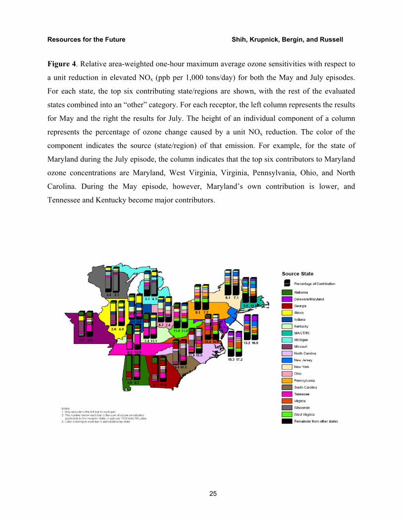
Figure 4. Relative area-weighted one-hour maximum average ozone sensitivities with respect to

a unit reduction in elevated NOx (ppb per 1,000 tons/day) for both the May and July episodes.

For each state, the top six contributing state/regions are shown, with the rest of the evaluated

states combined into an “other” category. For each receptor, the left column represents the results

for May and the right the results for July. The height of an individual component of a column

represents the percentage of ozone change caused by a unit NOx reduction. The color of the

component indicates the source (state/region) of that emission. For example, for the state of

Maryland during the July episode, the column indicates that the top six contributors to Maryland

ozone concentrations are Maryland, West Virginia, Virginia, Pennsylvania, Ohio, and North

Carolina. During the May episode, however, Maryland’s own contribution is lower, and

Tennessee and Kentucky become major contributors.

25


Figure 5. Relative area-weighted 24-hour average PM2.5 sensitivities with respect to a unit

reduction in total SO2 emissions (µg/m3 per 1,000 tons/day) for the May and July episodes. The

top six contributing state/regions and “all other states” are presented.

26

Documents

Source-Receptor Relationships for Ozone and Fine ... · PDF fileSource-Receptor Relationships for Ozone and Fine Particulates in the Eastern United States ... portion of this paper