Center for Environmental and Resource Economic Policy College of Agriculture and Life Sciences https://cenrep.ncsu.edu

Sooner or Safer? Bureaucracy in Oil and Gas Production

Eric C. Edwards, Trevor O’Grady, David Jenkins

Center for Environmental and Resource Economic Policy Working Paper Series: No. 19-017

March 2019

Suggested Citation: Edwards, Eric C., O’Grady, T., and D. Jenkins (2019). Sooner or Safer? Bureaucracy in Oil and Gas Production. (CEnREP Working Paper No. 19-017). Raleigh, NC: Center for Environmental and Resource Economic Policy.

Sooner or Safer? Bureaucracy in Oil and Gas Production

Eric C. Edwards, North Carolina State University1

Trevor O’Grady, The College of New Jersey

David Jenkins, Apache Corporation

March 15, 2019

Abstract:

Bureaucratic rules are implemented in organizations with limited direct financial incentives for agents to pursue the policy desired by the principal. However, these constraints can lead to inflexibility and delay. We examine the effect of bureaucratic rules on oil and gas drilling, production, and pollution in Wyoming using the allocation of alternating square-mile land sections to private owners via the Pacific Railroad Acts as a natural experiment. Subsequent to allocation, extensive natural gas extraction from the Green River Formation, undiscovered at the time the land was assigned, has occurred with only limited changes to the initial land assignment. Delay for drilling permits on federal land, attributable to compliance with the National Environmental Policy Act, is higher than on private land. Consistent with the anticipated effect of delay, federal lands in aggregate see reduced drilling and production relative to private parcels. However, federal lands see significantly lower rates of oil and water spills, even within individual companies drilling on both types of land, suggesting a tradeoff between permitting expediency and environmental protection.

Keywords: Bureaucracy, Regulation, Natural Experiment, Checkerboard, Oil, Natural Gas

JEL Codes: D73, P14, Q38, Q58, Q40

1 Please contact eric.edwards@ncsu.edu with questions regarding this manuscript. We would like to thank Ryan Kellogg, Tim Fitzgerald, Eric Lewis, James Evans, and Wally Thurman for their comments and suggestions. We would also like to thank participants at 2017 ASSA Meetings, 2017 AERE Summer Conference, 2017 UCSB Occasional Workshop, the Triangle Research in Environmental Economics seminar, and seminar attendees at Utah State University and Western Washington University for their feedback. We thank Tom Kropatsch, Jesse Prentice-Dunn, Mike Soraghan, and Kate Helm for sharing data and Benjamin Burger, Julie Lemaster, Riley Brinkerhoff, and Bob King for sharing their knowledge. A portion of this work was completed by David Jenkins as part of his master’s thesis at Utah State University funded by a Strata Policy fellowship. All errors are our own.

2

It is ironic that bureaucracy is still primarily a term of scorn, even though bureaus are among the most important institutions in every nation in the world. Not only do bureaus provide employment for a very significant fraction of the world’s population…, but also they make critical decisions which shape the economic, political, social, and even moral lives of nearly everyone on earth. Yet economists and political scientists have largely ignored bureaucratic decision making in constructing their theories of how the world operates.

-Anthony Downs “Inside Bureaucracy” (1964, p. 1)

I. Introduction

Governmental bureaucracy is often criticized for its inefficiency. Anecdotes of long waits for

decisions are common among citizens and firms interacting with US federal government agencies and

similar bureaucratic organizations. While significant attention has been paid in the economics literature to

how regulation can be enacted to reduce externalities, and its associated costs, less attention has been paid

to the bureaucracy associated with such regulations. Improving economic understanding of this area is

important, as central governmental spending is a large part of the modern economy, representing 30-60%

of GDP in OECD countries. Bureaucracies face an information asymmetry and principal-agent problem.

Policymakers rely on bureaucrats to allocate resources or services, but bureaucrats by the nature of their

position possess private information and policymakers must create mechanisms to ensure the allocation is

in line with their goals (McCubbins et al 1987; Gailmard and Patty 2012). This system differs from a

private market because bureaucrats do not have a direct financial incentive to allocate resources in an

efficient manner. For instance in the US Civil Service system, policymakers are expressly prohibited from

affecting the employment or compensation of most federal government employees (Johnson and Libecap

1994). Therefore, bureaucracies must be structured to ensure decisions are monitored: delay and caution

may be required to prevent misallocation (Prendergast, 2003). Public agencies structured with control

systems to monitor employees or standardized rules to reduce the cost of monitoring incur additional

costs, which are of interest to economists (Sunder 1998).

A central concern of the present paper is bureaucratic delay in making economic decisions. In

addition to the added time due to the control systems mentioned above, bureaucratic processes may be

3

delayed by bureaucrats shirking their responsibilities (McCubbins et al 1987); officials taking strategic

action to solicit bribes (Ahlin and Bose 2007; Fredriksson 2014); or by interest groups who benefit from

delay (Kosnik 2006). However, analysis of the cost of delay is hindered by the nature of governmental

agencies, which often provide goods and services that differ from their private counterparts. Further,

delay may itself be a part of the regulatory process; a careful bureaucratic accounting of a proposed rule

or regulation might lead to more socially beneficial outcomes (Carpenter et al 2012). For these reasons,

there is limited empirical work estimating how governmental bureaucracy affects economic outcomes or

exploring the channels through which additional costs arise.

In this paper we utilize a natural experiment that randomly assigns an identical task to bureaucratic

agencies and private firms. The task, oil and gas permitting, drilling, and extraction, is performed by a

federal governmental agency and private landowners. The expected benefits of the task and its potential

complexity are randomly assigned in the southern portion of the state of Wyoming via the allocation by

the US federal government of alternating square-mile sections to private owners via the Pacific Railroad

Acts between 1862 and 1871.2 To this day the area has retained much of the original pattern of land

allocation and is referred to as the “Wyoming Checkerboard.”

Our focus is on bureaucratic controls implemented by the federal government starting in the 1970s

that could alter the pattern of drilling and extraction. Federally owned lands have additional permitting

procedures to ensure compliance with federal environmental and conservation laws, which have over time

resulted in longer wait-times to drill on federal lands. In addition, federal lands have uniform royalty rates

and standardized leasing procedures to ensure agency compliance. In the 1970s, the allocation of oil and

gas leases on federal lands using lotteries with limited oversight drew significant criticism due to the

perception of malfeasance among competing firms and bureaucrats. The ensuing GAO investigation of

federal leasing policies resulted in policy changes (GAO 1979; Schmidt 1981; Haspel 1985). New federal

2 Of the lands retained by the federal government, every 16th and 36th square-mile section were allocated to the state government under the General Land Ordinance of 1785.

4

policies were implemented in the 1980s, culminating in the 1987 Federal Onshore Oil and Gas Leasing

Reform Act, which moved all federal leases to competitive bidding. Under the federal regime, significant

effort is made to ensure compliance with environmental and administrative procedure laws. This

difference in process relative to private lands may provide benefits as well as impose cost. In this paper,

we quantify cost of delay in oil and gas drilling due to bureaucratic restrictions and estimate the process’

resulting improvement in environmental performance.

We collect data on delay, drilling, production, and accidental spills in Wyoming, which produces

more gas from federal lands than any other US state, and likewise accounts for 36% of all onshore well

permit applications to the federal government.3 We focus our analysis on the Wyoming checkerboard,

centered on the Union-Pacific Railroad line that formed the first transcontinental railroad and overlying

valuable oil and gas fields in the Green River Formation, which were undiscovered at the time the land

was assigned and offer a unique natural experiment. Consistent with our understanding of bureaucratic

effects, we find: (i) Since the late 1980s, it takes longer to drill a well on federal lands; one year after

receiving approval to drill from the state of Wyoming, 23% of wells had not drilled on private land, but

that number rose to 58% on federal land. (ii) Delays reduce drilling on federal land; for the 2003-2015

period, private lands see yearly about 24 wells drilled per 1000 sections while federal lands see around

11. (iii) As a result, federal lands see less production than private lands; on average each federal section

produced a total of $4.6M from 1978-2015, while each private section produced $5.4M. (iv) There are

fewer oil and contaminated water spills on federal land; the rate of spills on federal land is about half that

on private land. The ability to avoid high costs associated with bureaucratic decisions is one argument

made for transferring lands owned by the US Federal Government to state or private control.4 We find

3 BLM data for the years 2008-2017, available at: https://www.blm.gov/programs/energy-and-minerals/oil-and-gas/oil-and-gas-statistics 4 E.g. http://publiclands.utah.gov/wp-content/uploads/2014/11/1.%20Land%20Transfer%20Analysis%20Final%20Report.pdf;

5

that while federal lands do see lengthy delays, the overall federal process reduces the likelihood of spills,

suggesting a key tradeoff between drilling efficiency and environmental protection.

Section II of the paper begins with a discussion of the institutional details of oil and gas extraction in

Wyoming and provides a predictive framework for the empirical analysis. Section III provides the

empirical strategy and section IV describes the data we use. Section V provides results and robustness

checks. A discussion follows in section VI and section VII concludes.

II. Background

a. Oil and Gas Permitting and Production

The United States is somewhat unique in the world in its assignment of ownership rights to minerals

to the overlying landowner, rather than the state or crown.5 In Wyoming, and the United States more

generally, oil and gas ownership is assigned via extraction, typically under a form of the correlative rights

doctrine. Regardless of overlying ownership, oil and gas sit below the surface in a common pool,

unclaimed until extraction. In Wyoming, mineral rights are held by private individuals, the state of

Wyoming, or the federal government. Landowners typically do not drill their own wells, and instead

drilling rights are leased to an extraction company. If oil or gas is produced, the landowner receives a

royalty payment, which is a percentage of the gross value of production (Fitzgerald and Rucker 2014). 6

Federal government parcels in Wyoming are managed by the Bureau of Land Management (BLM) and

are auctioned quarterly using a competitive sealed-bid first-price auction. Unsold leases are available to

be purchased non-competitively. Remaining parcels without a buyer are then recycled through the

5 For some land the federal government reserved its mineral rights, even as the overlying land was sold, creating “split-estate” where the ownership of land and right to drill for minerals rest with two different parties. 6 There is also a severance tax of 6% of production paid by all wells to the state of Wyoming, regardless of ownership.

6

auction.7 On BLM land, royalties paid to the Federal Government are 12.5%. In contrast, royalty rates on

private land are negotiated on a case-by-case basis. They average 15.3% (Brown et al 2016) but

demonstrate much greater variability, ranging up to 25% (Riley Brinkerhoff, pers. comm., 2015).8

Once a lease is secured, but prior to drilling, operators must apply for a permit to drill (APD) and

receive a Wyoming Oil and Gas Conservation Commission (WOGCC) permit (see WOGCC Rules and

Regulations 3(8)(a)). The only explicit environmental standard in the state guidelines, which apply to all

wells, is for the protection of groundwater (WOGCC 3(8)(c)). No on-site inspection or environmental

assessment is required to receive a permit. WOGCC has a stated goal of approving all permits within 30

days of receipt. In 2012, 78% of permits were approved within 30 days.9

Drilling on federal land requires a permit from the BLM in addition to the WOGCC permit. Under the

Mineral Leasing Act of 1920, which changed mineral claims on federal lands from land patents to leases,

there were limited requirements on mineral extraction and leasing. Increasing concern over environmental

and other impacts of productive activity on federal lands led to the National Historic Preservation Act

(NHPA) of 1966, the National Environmental Policy Act (NEPA) of 1970, and Endangered Species Act

(ESA) of 1973. In addition to environmental issues associated with federal oil and gas drilling, concerns

about the limited amount of production income from federal lands that was returned to taxpayers led to

the Federal Land Policy and Management Act of 1976. The Act required a systematic planning process

for federal lands including incorporation of physical, biological, economic, and other sciences in

determining potential uses and assessing environmental consequences.

A comparison of the timeline of leasing, permitting, drilling, and production processes for private and

federal lands is shown in Figure 1. There are two key differences in the processes: leasing and permitting.

7 Wyoming state leases are allocated in a similar manner through the Office of State Lands and Investments (OSLI), although the royalty rate and process for disposing of unsold leases differs. 8 Oil and gas operators secure a lease to land that has potential for oil and gas extraction via an upfront “bonus” payment to the landowner. Private lease duration is typically 3-5 years, state leases are set at 5 years (SBLC 2007), and nearly all federal leases in Wyoming have a duration of 10 years. The state of Wyoming charges royalties of 16.67% (SBLC 2007) 9 http://www-wsl.state.wy.us/slpub/strategic_plans/2013/2013_055_SP%20FY%2015_16.pdf

7

In general, land in the checkerboard is available to lease and, as discussed below, the data suggest that

there is not a difference in ADP applications by land type. We therefore focus our attention on the

permitting process as the key difference between private and federal lands. The duration of the federal

permitting process has been criticized by the Office of the Inspector General, which reported that in 2012

the average duration across all BLM offices to complete an application for a permit to drill (APD) was

228 days, even though 99% of all APDs were ultimately approved (Kendall 2014). The report suggests

that delays increase uncertainty, put royalties at risk, and can cause the cancellation of planned drilling

projects and suggests that federal drilling delays are due to processing time in addressing the requirements

of NEPA.

The process for receiving a permit to drill on federal land, including the NEPA process, is described

in great detail in the Surface Operating Standards and Guidelines for Oil and Gas Exploration and

Development, typically referred to as “The Gold Book” (BLM 2007). Requirements for permit approval

include the identification of “(l)evel of National Environmental Policy Act (NEPA) analysis required,”

and an on-site inspection by BLM agency representative to “identify site-specific concerns and potential

environmental impacts associated with the proposal; and discuss the conditions of approval (COAs) or

possible environmental Best Management Practices for mitigating these impacts.” The remainder of the

book describes, in great detail, construction requirements for oil and gas wells, environmental mitigation

requirements, and other regulatory requirements. The BLM permitting process is iterative. After an

operator submits an APD, deficiencies are identified for the operator to address. Data indicate that in most

years, the majority of delay is in operators addressing deficiencies in their APD.

Whether deficiencies will be found, and what an operator must do to address them, is viewed as

highly uncertain by operators. In written congressional testimony, Ryan Flynn, Executive Director the

New Mexico Oil and Gas Association, describes the issue: “The greatest challenge today is regulatory

uncertainty at BLM… the fact remains that operators are willing to pay a premium to develop in areas

where regulatory certainty can be relied upon as a matter of course.” The quote is consistent with the

GAO report; both suggest operators view the federal review process as uncertain and costly.

8

Once permits are secured and an oil or gas well is drilled, the extraction path is generally fixed and

output declines exponentially (Mason and Veld 2013). This means oil and gas production on producing

wells is highly price inelastic. The margin on which firms can respond to prices is in the number and type

of new wells brought online (Anderson et al. 2018). Oil rig activity, an indicator of exploration effort and

field development activity, increases with oil price, especially in North America due to the presence of

private firms and few government restrictions (Ringlund et al. 2008). The productivity of natural gas

production is almost entirely determined by geologic characteristics, with natural gas producers

responding to market prices through drilling (Mason and Roberts 2018). Natural gas reserve additions

through the drilling of new wells in West Virginia were consistent with this pattern as well, with the

elasticity of drilling and reserve additions positive with respect to wellhead price (Iledare 1995).

Empirically, for existing wells there is no positive price response of gas production using well-level data

(Newell et al 2016) or oil production using aggregate production data (Anderson et al. 2018).

From 2003 onward, non-conventional drilling approaches, including hydraulic fracturing, were

widely used across the United States and in Wyoming to extract “tight” oil and gas, which is located in

formations with low permeability.10 Although the checkerboard has not seen a meaningful amount of non-

conventional activity due to its geologic structure, the broader non-conventional regulatory environment

is relevant. While the BLM has proposed a rule that would more clearly define the requirements for

federal hydraulic fracturing, the rule is on hold due to ongoing litigation. Currently, operators must

submit an APD for a non-conventional well to the BLM in the same manner as for conventional wells.

The number of federal APD applications for onshore drilling increased dramatically as a result of the

hydraulic fracturing boom, from an average of 4,822 from 2001-2003 to 8,547 from 2004-2006,

potentially causing increased delay times for all federal applications (DOI 2012, p. 14.).

10 We define non-conventional extraction as any extraction in which a horizontal well is drilled.

9

b. Land Ownership

How land is owned and regulated has been shown to affect oil and gas production and contracting.

Balthrop and Schnier (2016) show that differing state policies in addressing common-pool issues affect

production decisions and Fitzgerald (2010) shows that where mineral and surface rights are split, bonus

payments are lower, reflecting additional costs of coordinating extraction. Leonard and Parker (2018) find

that federal (tribal) land is less productive around the Fort Berthold Indian Reservation in North Dakota as

a result of fragmented ownership leading to coordination problems for drilling non-conventional wells. In

these cases, it appears to be a particular policy or contracting problem affecting the economic outcome.

This is consistent with work on other resources where federal land managers have been shown to act

differently than private owners: timber sales on national forest lands (Repetto 1988); stocking decisions

on rangeland (Johnson and Watts 1989); and the organization of wildfire suppression activities (Lueck

2013). It is clear from these examples that federal and private land management outcomes differ. Less

clear is the cause of these differences, due to selection issues; it is not necessarily true in these examples

that the federal government is performing similar tasks on similar lands to private landowners because l

federal land is generally different than land that was claimed for private ownership, i.e. private owners

selected land, the federal government retained control over what remained.

In this paper we utilize the randomized allocation of federal lands due to the Pacific Railroad Acts

between 1862 and 1871, and state lands under the General Land Ordinance of 1785, to eliminate the land

selection issue. The acts granted title to every other section (1 mi2) of land within twenty miles of either

side of the Union-Pacific Railroad line that formed the first transcontinental railroad to Union-Pacific.

When Wyoming became a state, sections 16 and 36 in every township were granted to the state “for the

support of common schools.” (Wyoming Admission Act, 26 Stat. 222 § 4 1890), and many of those

sections were set aside as school trust lands. Today the Wyoming checkerboard overlies the Green River

Formation and underlying Mesozoic strata. In aggregate, each land type is likely to have the same

10

reservoir characteristics, geology, and production drive mechanisms because land is randomly allocated

and the area of most of the oil and gas pools is larger than one section (DeBruin, 1989).

The checkerboard has been used in several other economic studies: Ballaine (1953) discusses the

issues with checkerboard land grants for forest management in Oregon and Washington; Akee (2009)

examines a checkerboard allocation in an urban setting; Alston and Smith (2019) utilize the checkerboard

to understand the effect of fragmented land on irrigation investment; and Leonard and Plantinga (2018)

use the checkerboard allocation to help understand the economic effect of inaccessible federal lands.11

Figure 2 shows the federal surface estate and oil and gas producing areas from 1980-2010. The

Wyoming checkerboard and co-located (primarily) gas fields can be seen in the south-central and south-

western portions of the state. Lewis (2019) uses a similar approach to us in Wyoming to examine the

effect of spillovers due to federal environmental regulations, which he argues make exploratory drilling

more expensive on federal land. Using intent-to-treat design to assign state ownership to every 16th and

36th section, he finds preferential drilling on state relative to federal sections (in figure 2, these are the

federally owned areas around, but excluding, the checkerboard region). Interestingly, he finds evidence of

a spillover effect on federal lands, with exploratory drilling lower on federal land near state sections than

on federal land further away.12 While related to the work at hand, our approach differs and compliments

these findings, and other papers in this area, in three ways. First, our paper is focused on comparing

outcomes on federal relative to private land. Second, our paper identifies and ties the key cause of

bureaucratic rules to specific predictions about how rules will affect delay, drilling, and production. Third,

our paper is the first to explicitly test whether there are benefits to the environmental review process the

BLM undertakes.

11 It is relevant to note that the use of the Wyoming checkerboard as a natural experiment in oil and gas production was also undertaken by Kunce et al (2002) and Kunce et al (2004), but the results were retracted in both cases, by Gerking and Morgan (2007a) and Gerking and Morgan (2007b), respectively. 12 In a dissertation chapter, Lewis also examines the effects of private versus government ownership within the part of the Wyoming checkerboard that intersects the Green River Basin (Lewis 2015).

11

c. Predictions

Oil and gas drilling is a complicated contracting and engineering process. In comparing private and

federal lands, there are apparent differences in leasing, royalty rates, and permitting. Leasing, while an

important aspect of the overall process, occurs prior to the decision to drill and is therefore a sunk cost

that has a limited effect on firm production decisions. Royalty rates, on the other hand, could affect the

incentives of operators, but are similar in structure across private and federal lands and do not vary over

the modern time period on federal lands. We leave these topics, as well as other alternative mechanisms

that potentially explain differences across land types, to the discussion section. We focus on permitting,

and in particular the effect of the additional permit requirement to drill on federal land. We start with the

assumption that the additional permitting process for federal lands can only add delay to the process but

never subtract and therefore we predict:

Prediction 1: Due to additional permitting requirements, operators on federal land must wait longer to

begin drilling relative to private land.

As suggested by the Office of the Inspector General (Kendall 2014) and industry representatives, this

delay is potentially costly. An operator holding a lease to a particular section chooses to drill when the

expected rate of return of a well exceeds some hurdle rate determined by the operator. As oil or gas prices

rise, the expected return on the well increases. At the strike price, the hurdle rate is exceeded and drilling

begins. Because oil and gas prices are a random walk, for any well that sees a significant delay there is a

nonzero probability that the price has fallen below the strike price. For this reason, we predict:

Prediction 2: Longer expected delay makes drilling less likely on federal relative to private land, with

associated decreased aggregate production and revenue.

If prediction 2 holds, there will be some set of potential federal wells that are not drilled but which

would have been drilled on private land. These “missing” wells would have been the lowest productivity

12

federal wells. For this reason, we expect to see an effect on the average federal well in production, we

predict:

Prediction 3: Longer expected delay leads to higher average output on producing sections on federal

relative to private land.

Prediction 1 suggests that there will be delay in drilling on federal land as a result of the process by

which the federal government complies with the requirements of NEPA. In a cost-benefit analysis these

delay costs would be compared to any benefits the process causing a delay provides. We do not provide a

full accounting of costs and benefits, but can still examine observable environmental outcomes on federal

relative to private land. If the federal regulatory process provides environmental benefits, these are likely

to be observed in the rate at which spills occur.

Prediction 4: Holding production constant, fewer spills occur on federal relative to private land.

The remainder of the paper examines these predictions empirically. First, though, it is worth

examining when we expect the difference between federal and private outcomes to differ the most.

Because drilling is the key response to price, we expect most drilling activity, and thus the greatest

divergence between outcomes, to occur when prices are high or rising. Figure 3 provides an empirical

estimate of the incentive to drill in the Wyoming Checkerboard by providing a weighted price over time

based on the average well’s mix of oil and gas. After the market for natural gas was deregulated in the

1980s, natural gas prices remained relatively low until around 2000, when a sustained increase in price

began that would last until a combination of new supply spurred by the shale-gas boom (itself in part

driven by high gas prices) and decreasing economic activity as a result of the Great Recession lowered

price pressure. Given the price trend, the divergence in delay and production immediately around and

after the year 2000 is of particular interest to our empirical exploration.

13

III. Empirical Framework

We use the experimental setting created by the assignment of treatment types via the railroad

checkerboard in the 19th century. The transcontinental checkerboard pattern can be observed in figure 2

by looking closely at the states of Nevada and Wyoming, although in other areas the pattern has not

remained as distinct. Because oil and gas drilling did not start until the 20th century, the initial land

ownership allocation is independent of the quality of the oil and gas resource. To use this experiment

there are three potential regression strategies: (i) naïve regression: current ownership is used to compare

outcomes; (ii) intent-to-treat regression: parcels are characterized as retaining their original, random

ownership assignment; and (iii) instrumental variables regression: the checkerboard allocation is used as

an instrument for current ownership. Using current ownership is potentially problematic due to selection;

promising lands may have been claimed by private landowners due to their oil and gas potential. Both

other methods utilize exogenous assignment to identify the causal effect of ownership. The intent-to-treat

regression assumes all oil and gas extraction occurred under the initial pattern of ownership (this is the

approach used by Lewis (2019)), while instrumental variables regressions assume all the extraction

occurred under current ownership patterns, while using the original allocation as an instrument for current

holdings. The earlier parcels were transferred, the better the instrumental variables approximation of the

causal effect of the ownership regime.

Sections 16 and 36 within the checkerboard were allocated to the state of Wyoming through the

state’s Enabling Act. Because these state-allocated sections make up a small part of the checkerboard

sample and state lands are subject to rules that do not apply to federal or private land, we exclude these

sections from our analysis.

For the naïve regression, 𝑓𝑓𝑓𝑓𝑓𝑓𝑓𝑓𝑓𝑓𝑓𝑓𝑓𝑓 is a dummy variable representing current land ownership. The

dependent variable y for well i under land ownership j is related to federal ownership via the following

specification:

14

𝑦𝑦𝑖𝑖,𝑗𝑗 = 𝛼𝛼𝑛𝑛 + 𝛽𝛽𝑛𝑛𝑓𝑓𝑓𝑓𝑓𝑓𝑓𝑓𝑓𝑓𝑓𝑓𝑓𝑓𝑗𝑗 + 𝜖𝜖𝑖𝑖,𝑗𝑗 (1)

The coefficient 𝛽𝛽𝑛𝑛 represents the mean difference between federal and private ownership. However,

this specification does not control for ownership selection on characteristics related to the dependent

variable. The reduced form strategy, or intent-to-treat, uses 19th century land assignment as a direct

predictor of the dependent variable. The variable 𝑓𝑓𝑒𝑒𝑓𝑓𝑛𝑛 is an indicator for all even-numbered sections

(except 16 and 36), sections that were initially held in the public domain rather than given to railroad

companies. The reduced form estimating equation is:

𝑦𝑦𝑖𝑖,𝑗𝑗 = 𝛼𝛼𝑟𝑟𝑟𝑟 + 𝛽𝛽𝑟𝑟𝑟𝑟𝑓𝑓𝑒𝑒𝑓𝑓𝑛𝑛𝑖𝑖 + 𝜖𝜖𝑖𝑖,𝑗𝑗 (2)

Where 𝛽𝛽𝑟𝑟𝑟𝑟 represents the difference in the outcome variable between land initially allocated to federal

relative to private. The intent-to-treat regression models provide average causal effect estimates of the

initial ownership allocation on the outcome, rather than the effect of the actual ownership at the time the

outcome is determined. These two would be identical if the ownership allocation remained unchanged

over time.

Land characteristics appear balanced across the initial allocation, as can be seen in Table 1. Because

of the systematic assignment, this result is anticipated. Still, we examine whether factors that could affect

the choice to drill wells might have ended up different across the allocation. We include measures of

elevation and ruggedness, whether the endangered Sage Grouse has designated habitat in the area, and

known characteristics of the subsurface geology. Differences across the initial allocation are small and

statistically insignificant except that even sections are about ½ acre smaller on average. Although the

Public Land Survey System assigns land in a square grid, not all sections end up exactly 640 acres.

However, although statistically significant, in oil and gas drilling this small size difference is unlikely to

15

be economically relevant.13 The proportion of parcels inside each of the BLM’s “field office”

administrative unit boundaries are also virtually identical across assignment.

The top panel of figure 4 displays the instrument for ownership while the bottom panel displays

current ownership. Current ownership reflects the initial allocation of land via the checkerboard, but not

perfectly. Table 2 examines how current land ownership differs from the initial allocation pattern. Land

that was allocated to the railroads has largely, 97%, remained in private hands. However, fewer parcels,

76%, of initially retain public land remain under federal ownership today; some of these parcels were

claimed and converted to fee simple under various congressional acts. Much of the change in ownership

occurred through issuing private homesteads under the original Homestead Act of 1862 which transferred

ownership of surface and subsurface rights to the private owners. Homesteads were no longer settled

after 1940 and therefore the most substantial changes out of federal ownership occurred prior to oil and

gas production. For this reason we tend to prefer the IV specifications. Using two-stage least squares, our

first stage is:

𝑓𝑓𝑓𝑓𝑓𝑓𝑓𝑓𝑓𝑓𝑓𝑓𝑓𝑓𝑖𝑖,𝑗𝑗 = 𝜋𝜋0 + 𝜋𝜋1𝑓𝑓𝑒𝑒𝑓𝑓𝑛𝑛𝑖𝑖,𝑗𝑗 + 𝑢𝑢𝑖𝑖,𝑗𝑗 (3)

The second stage then uses the predicted value for federal to estimate equation (1):

𝑦𝑦𝑖𝑖,𝑗𝑗 = 𝛼𝛼𝑖𝑖𝑖𝑖 + 𝛽𝛽𝑖𝑖𝑖𝑖𝑓𝑓𝑓𝑓𝑓𝑓𝑓𝑓𝑓𝑓𝑓𝑓𝑓𝑓� 𝑖𝑖,𝑗𝑗 + 𝜖𝜖𝑖𝑖,𝑗𝑗 (4)

The specifications in equations (1)-(4) are written for regressions where the unit of observation is the

individual well, but are also applicable where the unit of observation is the square-mile section. Reported

standard errors are robust and typically clustered at the township level, and additional controls including

year, PLSS township (36 mi2), and firm specific fixed effects, as well as production controls (for spill

regressions) are used in primary specifications or robustness checks as discussed in the table notes and

where relevant in the discussion of the results.

13 A histogram of PLSS allocated section area in acres from the dataset we use is shown in figure A3. The vast majority of sections are around 640 acres.

16

IV. Data

Spatial GIS data and data from the WOGCC are used to characterize well-drilling and production in

Wyoming. We first construct a land ownership dataset using the Public Land Survey System (PLSS),

which typically is at the square-mile section, but smaller allocations are possible. We identify federal

subsurface ownership using the 2014 Surface Management Agency (SMA) shapefile from the BLM14 and

state subsurface ownership from the State Subsurface Ownership shapefile from the Wyoming Office of

State Lands and Investments.15 Subsurface rights that are not federally or state owned are assumed to be

privately owned.16 In the case of ownership areas smaller than the section, we assign ownership in

proportion to area owned by type. Because we are interested in land within the railroad checkerboard, we

use the first established transcontinental railroad route to estimate the boundaries of this allocation. We

use the 1870 railroads shapefile from the “Railroads and the Making of Modern America” project at the

University of Nebraska, Lincoln. The original checkerboard was established as a 20-mile buffer around a

proposed route of the Union Pacific Railroad (UPRR), which we do not observe, but the constructed route

was similar. To ensure that our sample is fully within the initial railroad grant, we restrict our data to

include sections within an 18-mile buffer around the 1870 UPRR route. As noted earlier, we drop all

sections allocated to the state of Wyoming, sections 16 and 36, from the data.

We use two datasets from WOGCC to identify the locations of wells, one on active wellheads and

one on permanently abandoned wellheads. Wells are individually identified by their API number, which

is a permanent identifier for every oil and gas well drilled in the United States. The dataset also provides

the PLSS information to link the wells to the section on which they are drilled. We link well data to the

land ownership data using PLSS information. We then use data on received and approved oil and gas

permits issued by the WOGCC from 1900-2015. Permits are required to drill on any land within

14 http://www.blm.gov/wy/st/en/resources/public_room/gis/datagis/state/state-own.html 15 States subsurface ownership last accessed 10/2016: http://gis.statelands.wyo.gov/osligis/oilandgas 16 We cross-check our private ownership designation with ownership information from sections with approved drilling permits (r=0.99).

17

Wyoming. Out of the roughly 100,000 approved permits in the data set, we are able to match 98% of

them to the GIS dataset and the section on which they are drilled. When we restrict permits to the

checkerboard area, we are left with 17,206 approved permits across 14,405 unique well locations.

While all wells require a WOGCC permit, drilling on federally owned subsurface areas requires an

additional permit from the BLM. We do not have data on BLM well permits, but can observe the approval

date of the WOGCC drilling permit and the spud date for each well.17 Because operators on federal land

need BLM approval before drilling, excess delay in federal permitting will increase the duration between

WOGCC permit approval and spud date for the well. Therefore, we define delay at the well-level as the

difference in time between the first WOGCC approved permit and the well spud date. WOGCC permits

expire if drilling has not started within 1 year of approval.18 Because application costs of permits are

relatively low, operators often fail to drill a well within a year of permit application and reapply. Most

well locations are associated with a single permit, however, some wells have up to as many as 9 approved

permits for a single well. We use date of the first application approval by the WOGCC as the permit

approval date. Because a fraction of permitted wells are never drilled, we measure whether or not a well

was drilled within 𝑥𝑥 days (30 days, 90 days, 1 year) of the first permit approval, so that the measure

includes approved wells that were not drilled. We also include a measure of the wells that were never

drilled, using December 31, 2015 as the end date. For wells that are ultimately drilled, we also construct a

measure of delay that is the number of days from permit approval to spud. All variables are described in

Table 3.

Delay is calculated for all wells with permit application information from 1900-2015. We break the

analysis into three periods based on the year in which the first permit for the well was approved: 1) 1900-

1986; 2) 1987-2002; and 3) 2003-2010. Period 1 represents a time of relatively slow production and

17 In fact, it is unclear whether the BLM has the data to analyze the length of permitting delays: "GAO found that BLM’s central oil and gas database was missing certain data...Without complete data on approved APDs, GAO could not perform a comprehensive assessment of the amount of time it took BLM to process APDs from their date of receipt to date of approval. (GAO 2013)" 18 Starting in January 2016 the WOGCC began allowing operators two years to start drilling before each permit expires, but this is outside the time frame of our data.

18

predates modern leasing requirements implemented in 1987. Period 2 represents the period of modern

leasing but predates the hydraulic fracturing boom.19 Period 3 covers starting dates for approved permits

during the hydraulic fracturing boom up until 2010. Our well production records continue through 2015,

providing a minimum five-year observation on whether wells are ever drilled.20

WOGCC production data is used to create a measure of wells drilled per section and aggregate

production measures for the amount of oil, natural gas, and water extracted. Because of mandatory

pooling at the section level, we aggregate all production data to the section level.21 To address the issue of

dynamic extraction, i.e. extraction in earlier periods affects current extraction decisions, production

measures are aggregated at the section for the entire period for which production data are available, 1978-

2015. In addition to the production of oil in barrels (Bbls), natural gas in thousands of cubic feet (Mcfs),

and water (Bbls), we construct revenue measures by multiplying production by monthly price. Price

information comes from two Energy Information Administration (EIA) datasets: Monthly US Wellhead

Gas Price and Monthly Wyoming Crude Oil Prices. We also calculate a combined measure of energy

production by converting the natural gas to a “barrel of oil equivalent” (BOE).

Finally, we obtain well spill reports from the WOGCC for years 1992-2015.22 Producers on all land

types are required to report spills that occur at the well to WOGCC. Since 2015, all reports are submitted

electronically via an online portal.23 Prior to 2015, companies were given the option of filing electronic or

paper reports.24 The data identifies the PLSS section where the spill occurred, the date, and the name of

19 The choice of 2003 as the start of the hydraulic fracturing boom follows Mason and Roberts (2018). 20 Of the 9,033 wells in the dataset for which we observe the time from permit approval to spud, only 43 take longer than five years to spud. 21 That is, only section-level production is observed and well-level production is calculated based on fixed proportions of section-level extraction from well tests. 22 The WOGCC is responsible for regulating spills that occur at the well, while any spills that occur during transport are regulated by the Wyoming Department of Environmental Quality. Chapter 4 Section 3 of the WOGCC Rules and Regulations requires a written report of all spills “of crude oil, condensate, produced water, or a combination thereof, which occur on a lease, unit, or communitized area” of more than one barrel (42 gallons). Reports must be filed as a written report within 15 working days of the spill. Industry sources report that any spill that requires a report is considered a major spill event. 23 See figure A1 in the appendix for the reporting interface. 24 Figure A2 shows a breakdown of reports by type, where known, and indicates that trends in reporting between land types generally appear consistent across methods of reporting.

19

the company, among other information. While the current online spill report form asks for the amount of

oil and water discharged, this data is not compulsory and was not recorded at all prior to 1999.

Unfortunately, discharge reporting is quite low, with only 4-16.5% of spill reporters in a given year

choosing to include discharge information. For this reason, we focus on the number of spills as the

indicator in our analysis. We aggregate spill data to the section and link to land ownership and production

data via PLSS section identifier. Because multiple companies may drill wells on a section but the spill

data is not linked to a specific well, we use the first company name by alphabetical order as the section

operator. For all sections that have production in a given year, we create a dummy variable equal to 1 if

there was a spill and 0 otherwise. This measures the rate at which a section spills (at least once) per year

without over-weighting sections that may have recorded multiple related spills.

V. Results

a. Delay

We begin with the prediction that delay to drill a well on federal land is longer than on private land.

Because BLM delay data is not available, we use a delay measure of the number of days from the date a

WOGCC permit is approved to the date a well is spudded. Figure 5 shows that the median number of

days for permit processing for WOGCC permits are similar across federal and private land (panel A), and

that generally all WOGCC permit applications are approved (panel B).25 Given that no differences in the

WOGCC permit process exist across land types, we proceed with the use of our proxy for delay. Median

delay between land allocated to federal and private landowners is shown in Figure 6, Panel A. Early on in

the sample the median delay time is 0 for both land types, meaning the well spud date and permit

approval date are the same for many observations. This suggests the same date was recorded for both and

that our measure of delay is not useful. However, our measure begins to capture a median delay in both

25 Appendix figure A4 shows the WOGCC permits received and granted for both federal and private lands. There are no clear differences in the rate at which the permits are approved.

20

land types starting around 1990, and shows increasing delay through 2010 on federally allocated land

relative to private land. Figure 6, Panel B shows the yearly difference in mean delay between these land

types with a 95% confidence interval. From 2000 on, the delay difference in a given year is statistically

significant at the 95% level. This corresponds to a period of increasing energy prices, as shown in figure

3, suggesting that delay is increasing as more permits to drill come in to BLM.26

We estimate the 2SLS regression from equations 3 and 4 for delay. Table 4 shows the results for

1900-1986, indicating little delay and no difference between federal and private land. However,

differences in delay are seen for the period 1987-2002 in Table 5. Specification (1) shows that around

78% of private wells are not drilled within 30 days of receiving a permit, with 90% of federal lands not

drilled within 30 days. Subsequent specifications are interpreted similarly. For instance, after one year,

wells with approved WOGCC permits on federal lands are 13 percentage points less likely to have had

been drilled. Table 6 shows results for the time period 2003-2010, with the magnitude of the coefficients

on federal land substantially higher than in the prior period. After one year, wells on federal land are 35

percentage points less likely to have been drilled than a well on private land.

To test the robustness of the delay results, we run both the naïve regressions, appendix tables A1-A3,

and reduced-form regressions, appendix tables A4-A6. Both sets of regressions show similar results to the

IV regressions encompassing the same time period. We also rerun the IV specifications using township

fixed effects, appendix tables A7-A9, with similar point estimates but lower statistical significance for

1987-2002, and nearly identical results for 2003-2010. Appendix figures A6-A9 provide alternative

measures of what constitutes a delay, all of which appear consistent with longer federal delay during the

permitting process. Figure A6 shows that there are small, but not systematic, differences in the time from

spud to well completion across land types, suggesting delay occurs in the permitting, and not the drilling,

26 Appendix figure A5 looks at the breakdown of WOGCC permits by the three BLM field offices that cover the checkerboard region. Panel A shows that basically all ADPs are approved, regardless of which area of the checkerboard they are in. Panel B shows the type of permit WOGCC receives for the area covered by each field office. The charts demonstrate consistency across the entire checkerboard in WOGCC permit processing and reviews.

21

phase of a well project. Figure A7 shows the rates over time of WOGCC permits that have expired prior

to drilling, with federal permit expirations exceeding those on private land starting in the late 1990s, but

especially after 2000. Figure A8 shows the proportion of permits never drilled, which is higher on federal

lands especially after 2000. Figure A9 shows the average number of times a permit is renewed prior to

approval. Recall that WOGCC permits expire after one year, so that if a well is permitted but not drilled

within a year, a renewal is required. Federal WOGCC permits are renewed more often before a well is

drilled than permits on private lands, with the largest divergence occurring for wells with their first permit

approved around or after 2000.

b. Drilling and Production

We next examine how well completions and production are affected by land ownership. Delay in

permitting on federal land is expected to decrease the number of wells drilled and overall average

production across all sections. Figure 7, Panel A shows a comparison of the average number of completed

wells per section by permit approval year. Panel B shows the total number of sections in production in a

given year. Similar to the delay results, there is a small divergence between federal and private lands in

the late 1990s, and starting around 2000 this difference becomes large. We run regressions examining

number of wells drilled per year per section, separating the regressions into the same time periods as in

the delay regressions. Results, shown in Table 7, indicate that in the period up to 1986, there are no

apparent differences in the number of wells drilled across ownership types. The difference becomes

statistically different for the period 1987-2002. The average private section sees about 0.01 wells drilled

in a given year (which can be seen in the figure but is not shown in regression due to the inclusion of time

fixed-effects), while the average federal section sees about 30% fewer wells drilled.

By the period 2003-2015, the number of wells added per section was about twice as high on private

land as federal, which is seen by comparing the coefficient on federal land of -0.0133 to the average

private section, which has an average well completion rate of 0.0245 wells per section per year (not

shown due to the inclusion of fixed effects). Per 1,000 sections, private lands see about 25 wells drilled

22

per year while federal lands have about 11. These results on federal relative to private land are consistent

with the delay results; no difference through 1986, longer delay and fewer wells on federal lands from

1987-2002, and the same pattern but larger coefficient estimated for 2003-2015.27

Turning to production, we use aggregate production per section across all years in the production

data, 1978-2015. In total, federal land produced $31.3B on 6,775 sections while private land produced

$41.5B on 7,615 sections. The per section average on federal lands, $4.6M, is lower than private lands at

$5.4M. We run regressions to statistically test the extent to which delay in permitting and drilling affect

aggregate production. Table 8 provides the results for all sections in the checkerboard. The average

private section sees more oil and gas production, resulting in higher revenue and more energy production.

For instance, specification (1) shows that a federal section produced 31.7% less revenue than a private

section.28

These regression results for federal land demonstrate the expected impact of delay on production and

drilling. The naïve regressions (shown in appendix table A12) do not show a negative coefficient on

federal land: controlling for selection into land ownership, rather than utilizing the naïve regression

approach is critical in this case, and will be even more important in comparing production in settings

where assignment is not as randomized as in the present case. Results for the reduced form (Table A14)

are similar to the IV-regression, and the divergence with the naïve regressions suggests that even the

relatively low percentage of parcels that have changed hands have done so in a way that is correlated with

gas production potential.29

In Table 9, we run the same production regressions, but limit the sample to sections that are actively

in production at some point from 1978-2015. Here, the coefficients are all positive, suggesting high

grading. In-production federal sections produced 43.2% more revenue than in-production private sections

27 Tables A10 and A11 in the appendix provide the results of the naïve and reduced form regressions 28 31.7% = (𝑓𝑓−0.3814 − 1) × 100 29 Table A16 also shows that the production results are robust to township fixed effects.

23

(by the coefficient in specification (1)).30 Turning to the robustness checks offers additional insight. The

inclusion of township fixed effects (Table A17) eliminates the observed statistical significance and

substantially reduces the point estimates. High-grading is primarily a between-township phenomenon;

within a given township, well outputs are relatively similar due to geologic similarities, but across

townships the average federal output is higher, indicating there are low-producing private lands where

nearby federal lands are not drilled.31

We can also include firm fixed effects in the regression, although because firms select into drilling a

particular type of land, this measure is not exogenous. However, we find that the point estimates remain

similar in magnitude and sign to the conditional production regressions, although the statistical power is

somewhat reduced as a result of including the large number of firms as explanatory variables (Tables

A18). This result suggests that high grading occurs within firms; individual firms drilling on multiple land

types react to the different regulatory regimes of each.

c. Spills

If the NEPA review and environmental regulatory framework is effective, the result should be the

improved environmental performance of wells once they are drilled on federal lands, relative to lands that

do not require the review. Figure 8 plots spills over time in the Wyoming checkerboard for land initially

allocated to federal and private owners. The y-axis in each panel is a spill rate, spills per section (panel A)

and spills per BOE (panel B), to scale the result to production. The trend across both types is a

consistently higher level of spills on private lands, relative to federal, per unit of production. Aggregate

spill counts by land allocation and section spill count (not shown) show similar trends. In aggregate, land

30 43.2% = (𝑓𝑓−0.3590 − 1) × 100 31 Conditional production regression results are also included for the naïve regression (table A13) and the reduced for regression (table A15).

24

allocated to private owners saw spills on about 2.70% of sections in production per year, and land

allocated to the federal government saw 1.27% of sections spill.32

We explore the effect statistically in order to control for current land ownership through the IV

specification. Table 10 shows the regression of whether a section spilled in a given year, and includes

several controls: number of wells on a section in the year the spill occurred; production in BOE the year

the spill occurred; and year and township fixed effects. The coefficient on federal land is consistently

negative and statistically significant. For instance, specification (6) shows that federal lands are about

1.44 percentage points less likely to see a spill, even controlling for both year and township fixed effects,

and total production. Both the naïve regression (Table A19) and the reduced form regression (Table A21)

show a similar, lower spill rate on federal lands.

One concern in interpreting the results of Table 10 is that certain firms may be absent from the data

set, for instance small firms who choose to drill on a particular land type may not have an effective

reporting and compliance system. Additionally, it would be interesting to understand the extent to which

the higher spill rates occur due to selection into drilling on a particular land type by safer (in terms of

spills) firms. We can shed light on these issues by using firm fixed effects in our regression. Because

which firm drills where is a potential outcome of land ownership, using it as a control could potentially

bias downwards the point estimate on land ownership. However, the results of these regressions, shown in

Table 11, suggest the spill rate difference occurs within firms. That is, for any given firm, the spill rate is

1.1-1.3 percentage points lower on federal relative to private land.33

32 Note that in the last year of the sample, 2015, the rate of spills on federal land increases and exceeds to rate on private lands, after a dramatic uptick in the number of spills on federally allocated lands. Although the uptick on federally allocated lands is large, it is much smaller on current federal lands (although it is still observable), suggesting it is perhaps spills on areas that have changed from federal allocation to private ownership that are driving results. It is difficult to speculate beyond this for one apparently anomalous data point, but it is suggestive that these trends are worth monitoring going forward. 33 Tables A20 and A22 show that the naïve and reduced form regressions arrive at similar coefficients for federal lands.

25

Based on the aggregate spill rates from the allocated parcels, the coefficients on federal indicate that

federal lands show about half the spill rate of private land. The firm fixed effect regressions provide us

with some confidence that the result is occurring due to land ownership, not firm type or differences in

the reporting system of different companies. Two new questions arise from these results: first, to what

extent is it the delay in federal review, versus other aspects of the regulatory environment, which reduces

spills? Second, to what extent are there potential spillovers from the federal regulatory regime, in

particular the shifting of tasks more likely to cause spills to move onto private land? Addressing these

questions empirically is beyond the scope of the present paper, but we return to a discussion of these

issues in the next section.

VI. Discussion

a. Delay, production and spills

In the proceeding sections, we have demonstrated that in oil and gas production, federal ownership

has two consequences relative to private ownership. The first is that the NEPA review process leads to

delay and thus fewer wells drilled and less production. For the 2003-2010 time period, approved state

permits on federal lands are 35 percentage points less likely to have been drilled within one year relative

to private lands. The result was the average private section was seeing about twice as many wells drilled

as the average federal section. Delay, and the resulting decrease in drilling activity on federal land, led to

less mineral extraction and overall revenue: the average federal section produced about 32% less revenue

than the average private section. However, due to a lack of drilling on the lowest low-productivity federal

sections, the average producing federal section was more productive than the average producing private

section. Because well production occurs for up to 30 or more years after drilling, the production measures

are somewhat backward looking. Wells drilled early in the sample period have produced more revenue to

the current date than wells drilled more recently. Relative delay has increased over time on federal lands,

26

and consequently the relative number of wells drilled has decreased. The full effect of this difference has

likely not fully impacted the aggregate production measures.

The second consequence of federal ownership is that a federal section is less likely to have a spill.

Federal sections in production are about 1.4 percentage points less likely to see a spill, controlling for the

yearly level of production on a section. Because the spill data starts in 1992, we are unable to link the

increased delay in federal permitting directly to differences in spill rates. Instead, we can suggest that the

overall regulatory regime on federal land, which includes a NEPA review process, leads to fewer spills.

This result is robust to firm fixed-effects, suggesting that it is adjustments within firms to drilling

requirements on federal lands that lead to fewer spills.

Our approach is limited by the relative nature of our analysis. To the extent that certain activities in

the production process need not take place at the point of extraction, it is possible operators may move

these off of federal lands. This type of spillover could occur, for instance, if wells on multiple sections

feed a single tank battery to aggregate produced oil, which is purposefully located off federal land. We

believe this issue is limited by the nature of the WOGCC spill data; spills which occur at a well or during

production are reported to WOGCC, but spills once the oil or gas is being transported are reported to the

Wyoming Department of Environmental Quality; our data is only the former.

b. Alternative explanations

We briefly explore four competing explanations for the observed empirical results, and suggest why

permitting delay remains the most plausible explanation for the observed patterns in the data.

Royalties: There are significant differences in contract structure between federal and private leases. The

royalty rate on all federal leases is fixed at 12.5% while private land is more flexible. A fixed royalty rate

could act like a severance tax, resulting in decreased production and high-grading on federal land

(Chakravorty et al 2010; Deacon 1993). However, much of the production on the checkerboard occurs

under unitization agreements, where contiguous fields are operated by a single operator who maximizes

aggregate value (Libecap and Wiggins 1985). An exploratory unit is typically formed prior to production,

27

and leaseholders within the unit receive a payout and bear cost proportionate to their stake in the unit,

typically determined by acreage, independent on whether a well is drilled on that acreage (Marranzino et

al). Thus, although lease structures differ, extraction decisions are made by the unit operator, not the

leaseholder and so individual royalty rates are not expected to impact oil and gas investment decisions on

unitized areas. However, within unit boundaries, underlying land ownership still determines whether or

not the parcel is affected by federal agency regulations and unit operators must apply for separate federal

permits to drill on federal land within a unit.

Leasing: As BLM and private landowners each have the option of opening or closing lands for lease, it is

possible that if the BLM closed certain lands, drilling and extraction would be affected. Although

occurring through a different pathway, this sort of outcome is consistent with the story of the study. Still,

our evidence does suggest the permitting mechanism as the key driver of the differences across land

types. Our delay measure begins after a lease has been signed and APD submitted, so any delay

attributable to pre-APD differences is not picked up in our delay measure. In addition, the observed high-

grading on federal land is consistent with a delay story but not a story where certain land is taken out of

the lease pool due to its environmental value or sensitivity. “Many of the lands closed to leasing consist of

areas with special designations and other unique and environmentally sensitive areas, such as habitat for

special status species (Kornze 2016).” It seems unlikely these criteria would selectively remove low-value

oil and gas deposits from the federal leasing pool while leaving high-value deposits available.

Bonding: Oil and gas extraction decisions are affected by bonding requirements. For instance, higher

bonding requirements in Texas caused small firms to exit the market and improved environmental

performance (Boomhower 2019). However, in Wyoming all wells face the same bonding requirements, as

the statewide bonding requirement for firms drilling multiple wells in the state and which applies to all

land types, is set at $100,000, which exceeds the minimum federal amount of $25,000.

Inspections: Federal and private inspection regimes may differ. Based on figure A5, which shows the

time from spud to well completion is similar across land types, we conclude that the observed delay is a

28

result of the ADP process, which as mentioned above includes at least one on-site inspection. But what

about differing inspection regimes as an explanation for the observed differences in spill rates. It is the

case that BLM conducts inspections of wells on federal lands and assesses penalties and fines if the wells

do not comply with regulations. For this reason, while the federal permitting process is related to the

difference in spill outcomes, it is not possible given our data to show a causal relationship. Indeed, it

appears that the spill rate difference has remained relatively static through time even as federal delay has

increased, suggesting it is not the delay itself that is preventing spills. Our empirical approach, however,

does not rely on a particular explanation for the difference in spills. Therefore, we can conclude that the

federal regulatory process, as a black box, is both effective at reducing spills and, when prices are rising

and APDs are increasing, can result in long delays. We now turn to estimating the opportunity cost of

these delays.

c. Lost profit per spill

Because the federal government’s review process has both apparent benefits and costs, it would be

useful to quantify the tradeoff. Although there are significant additional considerations in a full benefit-

cost analysis, estimating the opportunity cost of preventing spills through the current mechanism is a first

step, and within the scope of this paper. In making this calculation we do not observe cost directly, so we

assume a well-completion cost. Additionally, the missing wells on private land may be below-average

production wells, as indicated by the high-grading results on federal land. However, our spill data covers

a set of wells drilled more recently, for which production data is not complete. With these caveats, the

cost per spill prevented, CSP, is the difference in profit, Π, between land types divided by the difference

in spill rate, 𝜎𝜎:

𝐶𝐶𝐶𝐶𝐶𝐶 =Π𝑝𝑝𝑟𝑟𝑖𝑖 − Π𝑟𝑟𝑓𝑓𝑓𝑓𝜎𝜎𝑝𝑝𝑟𝑟𝑖𝑖 − 𝜎𝜎𝑟𝑟𝑓𝑓𝑓𝑓

=ΔΠΔ𝜎𝜎

=Δ𝑅𝑅 − Δ𝐶𝐶Δ𝜎𝜎

=Δ𝑅𝑅 − 𝐶𝐶𝑤𝑤𝑓𝑓𝑤𝑤𝑤𝑤 ⋅ Δ𝑊𝑊𝑓𝑓𝑓𝑓𝑓𝑓𝑊𝑊

Δ𝜎𝜎 (5)

The profit can be broken down into revenue, R, and cost, C. With the assumption that marginal cost

of extraction is nearly zero, we can substitute a constant cost of drilling a well into the calculation. We

29

estimate Δ𝜎𝜎 using the spill regression results shown in table 11. We choose to use specification (5) for our

point estimate, -0.0126 and construct a two standard-deviation confidence interval (-0.0190, -0.0062). We

run a regression similar to those in table 9, but using level of revenue, rather than log, and controlling for

township fixed-effects, to find that aggregate revenue was $1,027,127 higher for the average private

section. We run a regression similar to those shown in table 8, but for wells drilled for the entire period

1978-2015 and controlling for township FE, to find the average federal section had 0.1875 fewer wells

drilled over the time period. Assuming the cost to drill a well is around $5 million, we find over the 37

years, the average private section produced $89,627 more profit than the average federal section, or about

$2,422 more per year. Plugging this in as the numerator, we arrive at a point estimate cost of $192k

($127k; $391k) per avoided spill. This type of calculation is not a substitute for a full benefit-cost analysis

and depends on key assumptions about the cost of drilling a well, what years of data are used to calculate

spill rates, production differences, and well-drilling differences.34

VII. Conclusion

The paper’s results suggest that while there is a cost associated with delay, the bureaucratic regulatory

process is apparently effective at reducing oil and contaminated water spills. Our cost per spill estimate

could be used to answer the question: are the benefits of the bureaucratic review process worth the cost?

The lost profit on federal sections, at about $192k per avoided spill, could then be compared with the

environmental cost of the spills. This suggests that per unit of oil, marginal spill abatement cost is not

equalized across ownership types, nor even within firms, who spend more to prevent a spill on federal

land than on private land. The “problem” with bureaucracy is that it must create a costly set of internal

rules to ensure compliance of its agents. This system creates the issues we associate with bureaucracy

such as delay, inflexible processes, paperwork, and red tape. If the cost per spill prevented on federal land

is too high, perhaps private land owners choose the efficient level of spills and the regulatory process

34 While nicely summarizing the paper’s two main results into a clear tradeoff, the estimate itself relies on assumptions that did not receive the same rigorous analysis as the paper’s primary results, and should be interpreted accordingly.

30

constitutes waste. Alternatively, if private land owners require too little spill protection, it may be due to

lacking the regulatory ability or bargaining strength of the federal government. There is also a third

possibility, which is that the federal government, which represents all Americans, internalizes more of the

harm of spills, and chooses to implement correspondingly stricter rules.

Further research is needed to better quantify the cost of spills. In particular, it is likely that the

primary “spill” occurring on natural gas wells, the emission into the atmosphere of methane or other

airborne pollutants, does not show up in our data, except to the extent to which it is correlated with oil and

water spills. Although this paper is not able to fully quantify the tradeoff between bureaucratic delay and

pollution, its use of the railroad checkerboard as a natural experiment allows us to make a strong case for

a clear tradeoff existing between the more price-responsive drilling on private land and the safer

production of federal lands.

31

VIII. Sources

Ahlin, C. and Bose, P., 2007. Bribery, inefficiency, and bureaucratic delay. Journal of Development Economics, 84(1), pp.465-486.

Akee, R. (2009). Checkerboards and Coase: The Effect of Property Institutions on Efficiency in Housing Markets. Journal of Law and Economics, 52(2), 395-410.

Alston, E. and Smith, S.M. 2019. Development Derailed: Railroad Land Grants and Irrigation in the Western United States. Working Paper.

Anderson, S.T., Kellogg, R. and Salant, S.W., 2018. Hotelling under pressure. Journal of Political Economy, 126(3), pp.984-1026.

Ballaine, W.C., 1953. The Revested Oregon and California Railroad Grant Lands: A Problem in Land Management. Land Economics, 29(3), pp.219-232.

Balthrop, A.T. and Schnier, K.E., 2016. A regression discontinuity approach to measuring the effectiveness of oil and natural gas regulation to address the common-pool externality. Resource and Energy Economics, 44, pp.118-138.

Boomhower, J., 2019. Drilling Like There's No Tomorrow: Bankruptcy, Insurance, and Environmental Risk. American Economic Review, 109(2), pp.391-426.

Brown, J.P., Fitzgerald, T. and Weber, J.G., 2016. Capturing rents from natural resource abundance: Private royalties from US onshore oil & gas production. Resource and Energy Economics, 46, pp.23-38.

Bureau of Land Management (BLM). 2007. Surface Operating Standards and Guidelines for Oil and Gas Exploration and Development. BLM/WO/ST-06/021+3071/REV 07. Bureau of Land Management. Denver, Colorado. 84 pp.

Carpenter, D., Chattopadhyay, J., Moffitt, S. and Nall, C., 2012. The complications of controlling agency time discretion: FDA review deadlines and postmarket drug safety. American Journal of Political Science, 56(1), pp.98-114.

Chakravorty, U., Gerking, S.D., Leach, A. and Metcalf, G., 2010. State tax policy and oil production: The role of the severance tax and credits for drilling expenses. US Energy Tax Policy, pp.305-337.Coase, R.H., 1937. The nature of the firm. Economica, 4(16), pp.386-405.

Deacon, R.T., 1993. Taxation, depletion, and welfare: A simulation study of the US petroleum resource. Journal of environmental economics and management, 24(2), pp.159-187.

Department of the Interior (DOI). 2012. Oil and Gas Lease Utilization, Onshore and Offshore. US Department of the Interior Updated Report to the President. URL: https://www.doi.gov/sites/doi.gov/files/migrated/news/pressreleases/upload/Final-Report.pdf

DeBruin, R.H. 1989. Wyoming’s Oil and Gas Industry in the 1980's a Time of Change, WGS: Public Information Circular, No. 28

Downs, A. and Rand Corporation, 1967. Inside bureaucracy (p. 264). Boston: Little, Brown.

Fitzgerald, T., 2010. Evaluating split estates in oil and gas leasing. Land Economics, 86(2), pp.294-312.

Fitzgerald, T. and Rucker, R.R., 2014. US private oil and natural gas royalties: estimates and policy considerations. Available at SSRN 2442819.

32

Fredriksson, A., 2014. Bureaucracy intermediaries, corruption and red tape. Journal of Development Economics, 108, pp.256-273.

Gailmard, S. and Patty, J.W., 2012. Formal models of bureaucracy. Annual Review of Political Science, 15, pp.353-377.

GAO. 1979. “Onshore Oil and Gas Leasing--Who Wins the Lottery?” Report by the Comptroller General of the United States, Number EMD-79-41, April 14, 1979. URL: https://www.gao.gov/products/EMD-79-41

GAO. 2013. “Oil and Gas Development: BLM Needs Better Data to Track Permit Processing Times and Prioritize Inspections.” Report to Congressional Requesters, GAO-13-572, August 2013. URL: https://www.gao.gov/products/GAO-13-572

Gerking, S. and Morgan, W.E., 2007a. Effects of environmental and land use regulation in the oil and gas industry using the wyoming checkerboard as a natural experiment: Retraction. The American economic review, 97(3), p.1032.

Gerking, S. and Morgan, W.E., 2007b. Environmental and Land Use Regulation in Nonrenewable Resource Industries. Land Economics, 83(2), pp.iii-iii.

Haspel, A.E., 1985. Drilling for Dollars: The Federal Oil-Lease Lottery Program. Regulation, 9, p. 25.

Iledare, O.O., 1995. Simulating the effect of economic and policy incentives on natural gas drilling and gross reserve additions. Resource and energy economics, 17(3), pp.261-279.

Johnson, R.N. and Libecap, G.D. 1994. The Federal Civil Service System and the Problem of Bureaucracy. University of Chicago Press, Chicago, IL, pp.289.

Johnson, R.N. and Watts, M.J., 1989. Contractual stipulations, resource use, and interest groups: implications from federal grazing contracts. Journal of Environmental Economics and Management, 16(1), pp.87-96.

Kendall, M. 2014. Memo: Final Evaluation Report—Onshore Oil and Gas Permitting, U.S. Department of the Interior. Office of the Inspector General. Report No. CR-EV-MOA-0003-2013.

Kornze, N. 2016. “Recent Management of Oil and Gas Lease Sales by the Bureau of Land Management.” Director of Bureau of Land Management, U.S. Department of the Interior Testimony to the House Committee on Oversight and Government Reform Subcommittee on the Interior. URL: https://www.doi.gov/ocl/blm-lands-leasing

Kosnik, L.R.D., 2005. Sources of bureaucratic delay: a case study of FERC dam relicensing. Journal of Law, Economics, and Organization, 22(1), pp.258-288.

Kunce, M., Gerking, S. and Morgan, W., 2002. Effects of environmental and land use regulation in the oil and gas industry using the Wyoming checkerboard as an experimental design. The American Economic Review, 92(5), pp.1588-1593.

Kunce, M., Gerking, S. and Morgan, W., 2004. Environmental and land use regulation in nonrenewable resource industries: Implications from the Wyoming checkerboard. Land Economics, 80(1), pp.76-94.

Leonard, B. and Parker, D. 2018. Private vs. Government ownership of natural resources: evidence from the Bakken. Working Paper. URL: https://drive.google.com/file/d/1WFUycfRDZmM7lurRd4t1iv8qsxLCIy2T/view

33

Leonard, B. and Plantinga, A. 2019. "Stranded: The Effects of Inaccessible Public Land on Local Economies in the American West." Working Paper URL: https://drive.google.com/file/d/1zpqGCx0LLy5bpEVuGiFmsqu6-AFuAZsA/view

Lewis, E.K. 2019. Patchwork Policies, Spillovers, and the Search for Oil and Gas. American Economic Journal: Economic Policy. Forthcoming.

Lewis, E.K. 2015. Three Essays on the Economics of the Oil and Gas Industry. Dissertation. University of Michigan. URL: deepblue.lib.umich.edu/handle/2027.42/113565

Libecap, Gary D., and Steven N. Wiggins. 1985. "The influence of private contractual failure on regulation: the case of oil field unitization." Journal of Political Economy 93.4: 690-714.

Lueck, D., 2013. Economics and the Organization of Wildfire Suppression. In Wildfire Policy (pp. 87-104). Routledge.

Marranzino, T.A., Pink, J.B., Cavaleri, A.C. A primer on federal unitization, unit agreements and unit operating agreements. Anadarko Petroleum Corporation. URL: http://jay.law.ou.edu/faculty/Hampton/Mineral%20Title%20Examination/Spring%202012/Federal%20Unitization%20Primer%20Tom%20Marranzino.pdf

Mason, C.F. and van’t Veld, K., 2013. Hoteling Meets Darcy: A New Model of Oil Extraction. Working Paper. URL: http://www2.toulouse.inra.fr/lerna/seminaires/Hotelling_Darcy.pdf

Mason, C.F. and Roberts, G., 2018. Price Elasticity of Supply and Productivity: An Analysis of Natural Gas Wells in Wyoming. The Energy Journal, 39(S1), pp.79-101.

McCubbins, M.D., Noll, R.G. and Weingast, B.R., 1987. Administrative procedures as instruments of political control. Journal of Law, Economics, & Organization, 3(2), pp.243-277.

Newell, R.G., Prest, B.C. and Vissing, A., 2016. Trophy Hunting vs. Manufacturing Energy: The Price-Responsiveness of Shale Gas (No. w22532). National Bureau of Economic Research.

Prendergast, C., 2003. The limits of bureaucratic efficiency. Journal of Political Economy, 111(5), pp.929-958.

Ringlund, G.B., Rosendahl, K.E. and Skjerpen, T., 2008. Does oilrig activity react to oil price changes? An empirical investigation. Energy Economics, 30(2), pp.371-396.

Repetto, R. (1988). Subsidized timber sales from national forest lands in the United States. In R. Repetto & M. Gillis (Eds.), Public Policies and the Misuse of Forest Resources (pp. 353-384). Cambridge: Cambridge University Press. doi:10.1017/CBO9780511601125.009

Schmidt, William E. 1981. “Long-Shot Oil Lease Lottery A Bonus in Wyoming.” New York Times, September 30, 1981, Page A00020 URL: https://www.nytimes.com/1981/09/30/us/long-shot-oil-lease-lottery-a-bonus-in-wyoming.html

Sunder, Shyam. 1998. “Structure of Organizations for Production of Public and Private Goods , Yale School of Management Working Paper URL: http://www.som.yale.edu/Faculty/sunder/AAAPresentation/public.pdf

State Board of Land Commissioners (SBLC). 2007. Rules and regulations: board of land commissioners: Chapter 18: Leasing of Oil and Gas. URL: http://lands.wyo.gov/resources/rulesandpolicies

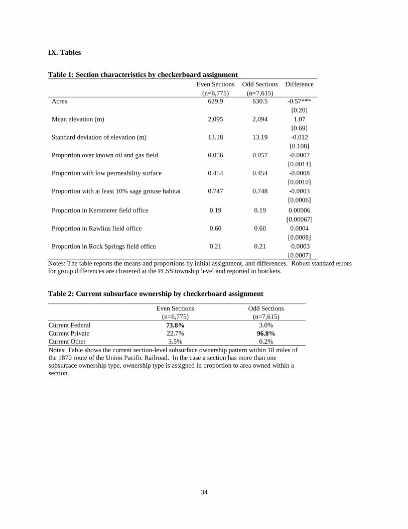
34

IX. Tables

Table 1: Section characteristics by checkerboard assignment Even Sections Odd Sections Difference (n=6,775) (n=7,615) Acres 629.9 630.5 -0.57***

[0.20] Mean elevation (m) 2,095 2,094 1.07 [0.69] Standard deviation of elevation (m) 13.18 13.19 -0.012 [0.108] Proportion over known oil and gas field 0.056 0.057 -0.0007 [0.0014] Proportion with low permeability surface 0.454 0.454 -0.0008 [0.0010] Proportion with at least 10% sage grouse habitat 0.747 0.748 -0.0003 [0.0006] Proportion in Kemmerer field office 0.19 0.19 0.00006 [0.00067] Proportion in Rawlins field office 0.60 0.60 0.0004 [0.0008] Proportion in Rock Springs field office 0.21 0.21 -0.0003 [0.0007]

Notes: The table reports the means and proportions by initial assignment, and differences. Robust standard errors for group differences are clustered at the PLSS township level and reported in brackets.

Table 2: Current subsurface ownership by checkerboard assignment

Even Sections Odd Sections (n=6,775) (n=7,615) Current Federal 73.8% 3.0% Current Private 22.7% 96.8% Current Other 3.5% 0.2% Notes: Table shows the current section-level subsurface ownership pattern within 18 miles of the 1870 route of the Union Pacific Railroad. In the case a section has more than one subsurface ownership type, ownership type is assigned in proportion to area owned within a section.

35

Table 3: Variables Used in Empirical Analysis Variable Description Source 𝑓𝑓𝑓𝑓𝑓𝑓𝑓𝑓𝑓𝑓𝑓𝑓𝑓𝑓 =1 if section i has federal mineral ownership as of 2016 BLM 𝑊𝑊𝑠𝑠𝑓𝑓𝑠𝑠𝑓𝑓 =1 if section i has state mineral ownership as of 2016 WOSLI 𝐷𝐷𝑓𝑓𝑖𝑖𝑓𝑓𝑛𝑛 =1 if section i is even, not 16 or 36 Authors’ calculation 𝐷𝐷16,36 =1 if section i is 16 or 36 Authors’ calculation 𝑛𝑛𝑛𝑛𝑊𝑊𝑛𝑛𝑢𝑢𝑓𝑓30 Proportion of permitted wells of ownership j not spudded within

30 days WOGCC

𝑛𝑛𝑛𝑛𝑊𝑊𝑛𝑛𝑢𝑢𝑓𝑓90 Proportion not spudded within 90 days WOGCC 𝑛𝑛𝑛𝑛𝑊𝑊𝑛𝑛𝑢𝑢𝑓𝑓365 Proportion not spudded within one year WOGCC 𝑛𝑛𝑛𝑛𝑊𝑊𝑛𝑛𝑢𝑢𝑓𝑓 Proportion that are never spudded WOGCC 𝑓𝑓𝑓𝑓𝑓𝑓𝑓𝑓𝑦𝑦 Given a well is ultimately drilled, days from approval to spud WOGCC 𝑛𝑛𝑖𝑖𝑓𝑓 Total oil production, sum for entire section 1978-2015 WOGCC 𝑔𝑔𝑓𝑓𝑊𝑊 Total gas production, sum for entire section 1978-2015 WOGCC 𝑤𝑤𝑓𝑓𝑠𝑠𝑓𝑓𝑓𝑓 Total water production, sum for entire section 1978-2015 WOGCC 𝑛𝑛𝑖𝑖𝑓𝑓𝑓𝑓𝑓𝑓𝑒𝑒𝑓𝑓𝑛𝑛𝑢𝑢𝑓𝑓 Sum of oil revenue (monthly production times price) for an

entire section 1978-2016 WOGCC and EIA

𝑔𝑔𝑓𝑓𝑊𝑊𝑓𝑓𝑓𝑓𝑒𝑒𝑓𝑓𝑛𝑛𝑢𝑢𝑓𝑓 Sum of gas revenue (monthly production times price) for an entire section 1978-2016

WOGCC and EIA

𝑠𝑠𝑛𝑛𝑠𝑠𝑓𝑓𝑓𝑓𝑓𝑓𝑓𝑓𝑒𝑒𝑓𝑓𝑛𝑛𝑢𝑢𝑓𝑓 Sum of oil and gas revenue WOGCC and EIA 𝑓𝑓𝑛𝑛𝑓𝑓𝑓𝑓𝑔𝑔𝑦𝑦 Barrels of oil equivalent: oil prod + (gas prod)/6 Authors’ calculation 𝑊𝑊𝑛𝑛𝑖𝑖𝑓𝑓𝑓𝑓𝑊𝑊 Number of spills on a section, yearly, 1992-2015 WOGCC 𝑤𝑤𝑓𝑓𝑓𝑓𝑓𝑓𝑊𝑊 Number of wells drilled on a section, yearly, 1978-2016 Authors’ calculation 𝑐𝑐𝑛𝑛𝑐𝑐𝑛𝑛𝑓𝑓𝑛𝑛𝑦𝑦 Listed well operator WOGCC

36

Table 4: Second-Stage IV Regression of Delay from State Permit Approval to Drilling (1900-1986) (1) (2) (3) (4)

Predicted Probability Current Ownership

No Spud after 30

Days

No Spud after 90

Days No Spud

after 1 year Never Spud Federal -0.02 -0.01 0.02* 0.01

[0.01] [0.01] [0.01] [0.01]

Constant 0.13*** 0.08*** 0.04*** 0.03*** [0.01] [0.01] [0.01] [0.01]

Observations 3,643 3,643 3,643 3,643 Notes: The table shows 2nd-stage regression estimates of the probability that (first) permit to spud time exceeds the threshold specified in each column on current ownership type instrumented by initial ownership type. Robust standard errors clustered at the PLSS township level in brackets. *** p<0.01, ** p<0.05, * p<0.1

Table 5: Second-Stage IV Regression of Delay from State Permit Approval to Drilling (1987-2002)

(1) (2) (3) (4)

Predicted Probability Current Ownership

No Spud after 30

Days

No Spud after 90

Days No Spud

after 1 year Never Spud Federal 0.12*** 0.20*** 0.13*** 0.08***

[0.02] [0.03] [0.03] [0.03]

Constant 0.78*** 0.47*** 0.27*** 0.20*** [0.02] [0.02] [0.03] [0.02]

Observations 2,844 2,844 2,844 2,844 Notes: The table shows 2nd-stage regression estimates of the probability that (first) permit to spud time exceeds the threshold specified in each column on current ownership type instrumented by initial ownership type. Robust standard errors clustered at the PLSS township level in brackets. *** p<0.01, ** p<0.05, * p<0.1

37

Table 6: Second-Stage IV Regression of Delay from State Permit Approval to Drilling (2003-2010) (1) (2) (3) (4)

Predicted Probability Current Ownership

No Spud after 30

Days No Spud

after 90 Days No Spud

after 1 year Never Spud Federal 0.13*** 0.35*** 0.35*** 0.20***

[0.03] [0.04] [0.03] [0.04]

Constant 0.84*** 0.55*** 0.23*** 0.16*** [0.03] [0.03] [0.03] [0.02]

Observations 3,737 3,737 3,737 3,737 Notes: The table shows 2nd-stage regression estimates of the probability that (first) permit to spud time exceeds the threshold specified in each column on current ownership type instrumented by initial ownership type. Robust standard errors clustered at the PLSS township level in brackets. *** p<0.01, ** p<0.05, * p<0.1

Table 7: Second-Stage IV Regression of Wells Drilled (1) (2) (3)

Years 1900-1986 1987-2002 2003-2015 Federal 0.0004 -0.0034*** -0.0133***

[0.0004] [0.0007] [0.0027]

Observations 1,251,930 230,240 187,070 Notes: The table shows 2nd-stage regression estimates of the number of wells drilled on a section in a given year. All regressions include year fixed effects. Robust standard errors clustered at the PLSS township level in brackets. *** p<0.01, ** p<0.05, * p<0.1

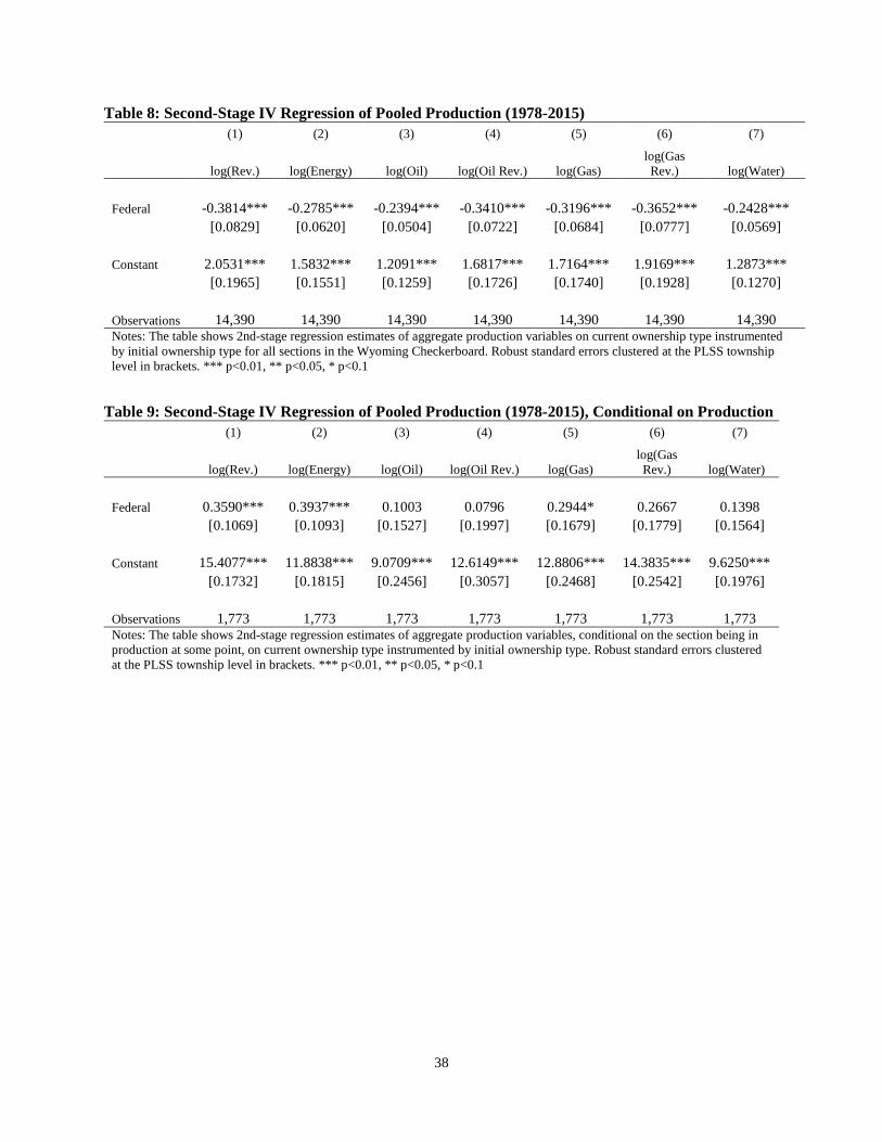
38

Table 8: Second-Stage IV Regression of Pooled Production (1978-2015) (1) (2) (3) (4) (5) (6) (7)

log(Rev.) log(Energy) log(Oil) log(Oil Rev.) log(Gas) log(Gas Rev.) log(Water)

Federal -0.3814*** -0.2785*** -0.2394*** -0.3410*** -0.3196*** -0.3652*** -0.2428***

[0.0829] [0.0620] [0.0504] [0.0722] [0.0684] [0.0777] [0.0569]

Constant 2.0531*** 1.5832*** 1.2091*** 1.6817*** 1.7164*** 1.9169*** 1.2873***

[0.1965] [0.1551] [0.1259] [0.1726] [0.1740] [0.1928] [0.1270]

Observations 14,390 14,390 14,390 14,390 14,390 14,390 14,390 Notes: The table shows 2nd-stage regression estimates of aggregate production variables on current ownership type instrumented by initial ownership type for all sections in the Wyoming Checkerboard. Robust standard errors clustered at the PLSS township level in brackets. *** p<0.01, ** p<0.05, * p<0.1

Table 9: Second-Stage IV Regression of Pooled Production (1978-2015), Conditional on Production (1) (2) (3) (4) (5) (6) (7)

log(Rev.) log(Energy) log(Oil) log(Oil Rev.) log(Gas) log(Gas Rev.) log(Water)

Federal 0.3590*** 0.3937*** 0.1003 0.0796 0.2944* 0.2667 0.1398

[0.1069] [0.1093] [0.1527] [0.1997] [0.1679] [0.1779] [0.1564]

Constant 15.4077*** 11.8838*** 9.0709*** 12.6149*** 12.8806*** 14.3835*** 9.6250***

[0.1732] [0.1815] [0.2456] [0.3057] [0.2468] [0.2542] [0.1976]

Observations 1,773 1,773 1,773 1,773 1,773 1,773 1,773 Notes: The table shows 2nd-stage regression estimates of aggregate production variables, conditional on the section being in production at some point, on current ownership type instrumented by initial ownership type. Robust standard errors clustered at the PLSS township level in brackets. *** p<0.01, ** p<0.05, * p<0.1

39

Table 10: Spill Analysis Results (1) (2) (3) (4) (5) (6)

VARIABLES Section Spilled

Section Spilled

Section Spilled

Section Spilled

Section Spilled

Section Spilled

Federal -0.0145*** -0.0134*** -0.0141*** -0.0164*** -0.0144*** -0.0152***

[0.0028] [0.0027] [0.0028] [0.0030] [0.0029] [0.0029] Per 1000 Wells 0.3881*** 0.4210***

[0.0925] [0.1065] Per Million BOE 0.0391 0.0644*

[0.0307] [0.0380]

Observations 26,237 26,237 26,237 26,237 26,237 26,237 Fixed Effects Year Year Year Year, Twsp Year, Twsp Year, Twsp Notes: The table shows 2nd-stage regression estimates of whether a section had a spill in a given year (1992-2015), conditional on the section being in production, on current ownership type instrumented by initial ownership assignment. Robust standard errors clustered at the PLSS township level in brackets. *** p<0.01, ** p<0.05, * p<0.1

Table 11: Spill Analysis Results with Firm Fixed-Effects (1) (2) (3) (4) (5) (6)

VARIABLES Section Spilled

Section Spilled

Section Spilled

Section Spilled

Section Spilled

Section Spilled

Federal -0.0129 -0.0116*** -0.0123*** -0.0151*** -0.0126*** -0.0133***

[0.0000] [0.0028] [0.0029] [0.0034] [0.0032] [0.0032] Per 1000 Wells 0.4319*** 0.4440***

[0.0930] [0.1137] Per Million BOE 37,792 73,730*

[32,384] [40,476]

Observations 26,237 26,237 26,237 26,237 26,237 26,237

Fixed Effects Year, Firm Year, Firm Year, Firm

Year, Twsp, Firm

Year, Twsp, Firm

Year, Twsp, Firm

Notes: The table shows 2nd-stage regression estimates of whether a section had a spill in a given year (1992-2015), conditional on the section being in production, on current ownership type instrumented by initial ownership assignment. All regressions include controls for firm fixed effects. Robust standard errors clustered at the PLSS township level in brackets. *** p<0.01, ** p<0.05, * p<0.1

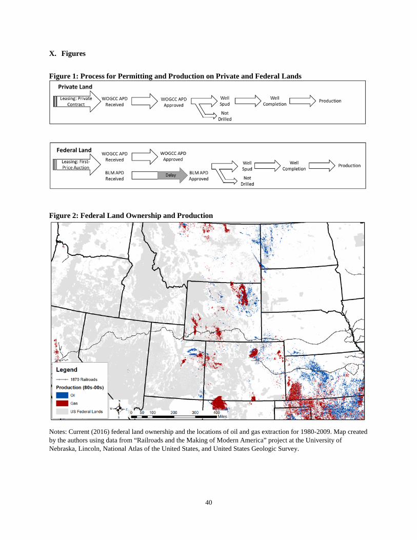
40

X. Figures

Figure 1: Process for Permitting and Production on Private and Federal Lands

Figure 2: Federal Land Ownership and Production

Notes: Current (2016) federal land ownership and the locations of oil and gas extraction for 1980-2009. Map created by the authors using data from “Railroads and the Making of Modern America” project at the University of Nebraska, Lincoln, National Atlas of the United States, and United States Geologic Survey.

41

Figure 3: Expected Real Revenue of Drilling in Wyoming

Notes: Expected revenue is determined by a weighted average of oil and gas prices per barrel of oil equivalent. Weights are based on the proportion of energy from oil (0.15) and gas (0.85) for all production from 1978-2015 within the Wyoming Checkerboard region.

42

Figure 4: Land Allocation and Ownership in the Wyoming Checkerboard

Notes: Instrument for original land allocation (top) and current subsurface land ownership (bottom). Ownership information displayed only within 18-mile buffer of 1870 railroad. Map created by the authors using data from “Railroads and the Making of Modern America” project at the University of Nebraska, Lincoln, Bureau of Land Management, and Wyoming State Office of Land and Investments.

43

Figure 5: WOGCC permit requests and approvals

A B

Notes: Panel A plots median number of days from when an application is received by WOGCC to when it is approved, conditional on the initial allocation of land (instrument). Panel B shows the difference in the total number of permit applications received and approved in a given year. Figure 6: Time from State Permit Approval to Spud A B

Notes: Panel A plots median days from state permit approval to spud by initial ownership allocation (instrument) for each year. Panel B shows the difference in means associated with federal land relative to private with 95% confidence intervals for the same variable. Approved APDs that never go to spud were excluded in the calculation of median and mean differences.

44

Figure 7: Wells Drilled and Active Wells A B

Notes: Panel A plots wells spudded per section by state permit approval year, conditional on the initial allocation of land (instrument). Panel B shows number of sections with an actively producing well in that year by initial allocation.

Figure 8: Spill Rates by Allocated Land Type A B

Notes: Plots of WOGCC spill data over time by original land allocation (instrument) from 1992-2015. Panel A plots the number of spills per producing section and Panel B the number of spills per barrel of oil equivalent.

.02

.04

.06

.08

.1Pr

opor

tion

of S

ectio

ns w

ith a

n Ac

tive

Wel

l

1980 1990 2000 2010 2020Production Year

Federal Private

45

XI. Appendix Tables

Table A1: Naïve Regression of Delay from State Permit Approval to Drilling (1900-1986) (1) (2) (3) (4)

Predicted Probability Current Ownership

No Spud after 30

Days

No Spud after 90

Days No Spud

after 1 year Never Spud Federal -0.02 -0.01 0.02* 0.01

[0.01] [0.01] [0.01] [0.01]

Constant 0.13*** 0.08*** 0.04*** 0.03*** [0.01] [0.01] [0.01] [0.01]

Observations 3,643 3,643 3,643 3,643 R-squared 0.00 0.00 0.00 0.00 Notes: The table shows OLS regression estimates of the probability that (first) permit to spud time exceeds the threshold specified in each column on current ownership type. Robust standard errors clustered at the PLSS township level in brackets. *** p<0.01, ** p<0.05, * p<0.1

Table A2: Naïve Regression of Delay from State Permit Approval to Drilling (1987-2002) (1) (2) (3) (4)

Predicted Probability Current Ownership

No Spud after 30

Days

No Spud after 90

Days No Spud

after 1 year Never Spud Federal 0.15*** 0.21*** 0.13*** 0.07**

[0.02] [0.03] [0.03] [0.03]

Constant 0.77*** 0.47*** 0.27*** 0.20*** [0.02] [0.02] [0.02] [0.02]

Observations 2,844 2,844 2,844 2,844 R-squared 0.04 0.04 0.02 0.01 Notes: The table shows OLS regression estimates of the probability that (first) permit to spud time exceeds the threshold specified in each column on current ownership type. Robust standard errors clustered at the PLSS township level in brackets. *** p<0.01, ** p<0.05, * p<0.1

46

Table A3: Naïve Regression of Delay from State Permit Approval to Drilling (2003-2010) (1) (2) (3) (4)

Predicted Probability Current Ownership

No Spud after 30

Days No Spud

after 90 Days No Spud

after 1 year Never Spud Federal 0.14*** 0.34*** 0.33*** 0.18***

[0.03] [0.03] [0.03] [0.04]

Constant 0.84*** 0.55*** 0.24*** 0.17*** [0.03] [0.03] [0.03] [0.02]

Observations 3,737 3,737 3,737 3,737 R-squared 0.05 0.13 0.11 0.04 Notes: The table shows OLS regression estimates of the probability that (first) permit to spud time exceeds the threshold specified in each column on current ownership type. Robust standard errors clustered at the PLSS township level in brackets. *** p<0.01, ** p<0.05, * p<0.1

47

Table A4: Reduced Form Regression of Delay from State Permit Approval to Drilling (1900-1986) (1) (2) (3) (4)

Predicted Probability Current Ownership

No Spud after 30

Days

No Spud after 90

Days No Spud

after 1 year Never Spud Federal -0.02 -0.01 0.02* 0.01

[0.01] [0.01] [0.01] [0.01]

Constant 0.13*** 0.08*** 0.04*** 0.03*** [0.01] [0.01] [0.01] [0.01]

Observations 3,643 3,643 3,643 3,643 R-squared 0.00 0.00 0.00 0.00 Notes: The table shows OLS regression estimates of the probability that (first) permit to spud time exceeds the threshold specified in each column on initial ownership assignment. Robust standard errors clustered at the PLSS township level in brackets. *** p<0.01, ** p<0.05, * p<0.1

Table A5: Reduced Form Regression of Delay from State Permit Approval to Drilling (1987-2002) (1) (2) (3) (4)

Predicted Probability Current Ownership

No Spud after 30

Days

No Spud after 90

Days No Spud

after 1 year Never Spud Federal 0.11*** 0.18*** 0.12*** 0.07**

[0.02] [0.03] [0.03] [0.03]

Constant 0.78*** 0.47*** 0.27*** 0.20*** [0.02] [0.02] [0.03] [0.02]

Observations 2,844 2,844 2,844 2,844 R-squared 0.02 0.03 0.02 0.01 Notes: The table shows OLS regression estimates of the probability that (first) permit to spud time exceeds the threshold specified in each column on initial ownership assignment. Robust standard errors clustered at the PLSS township level in brackets. *** p<0.01, ** p<0.05, * p<0.1

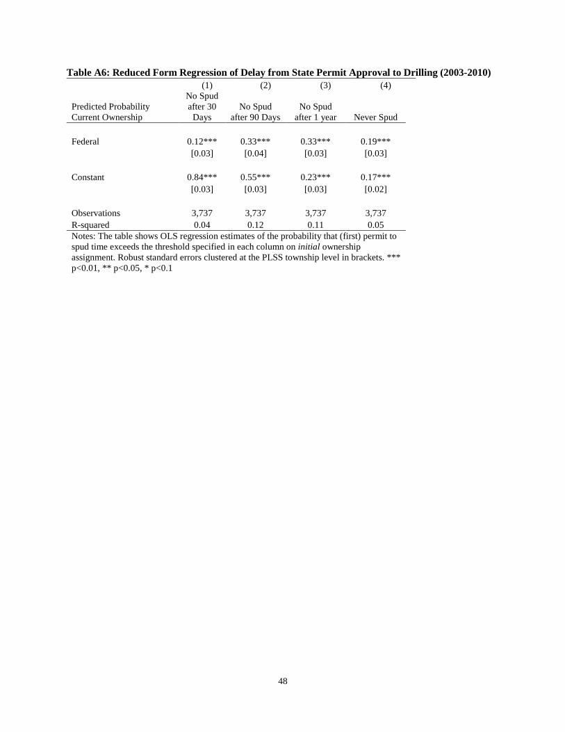
48

Table A6: Reduced Form Regression of Delay from State Permit Approval to Drilling (2003-2010) (1) (2) (3) (4)

Predicted Probability Current Ownership

No Spud after 30

Days No Spud

after 90 Days No Spud

after 1 year Never Spud Federal 0.12*** 0.33*** 0.33*** 0.19***

[0.03] [0.04] [0.03] [0.03]

Constant 0.84*** 0.55*** 0.23*** 0.17*** [0.03] [0.03] [0.03] [0.02]

Observations 3,737 3,737 3,737 3,737 R-squared 0.04 0.12 0.11 0.05 Notes: The table shows OLS regression estimates of the probability that (first) permit to spud time exceeds the threshold specified in each column on initial ownership assignment. Robust standard errors clustered at the PLSS township level in brackets. *** p<0.01, ** p<0.05, * p<0.1

49

Table A7: Second-Stage IV Regression of Delay from State Permit Approval to Drilling (1900-1986) with Township Fixed Effects

(1) (2) (3) (4)

Predicted Probability Current Ownership

No Spud after 30

Days

No Spud after 90

Days No Spud

after 1 year Never Spud Federal -0.02 -0.01 0.01 0.00

[0.00] [0.00] [0.00] [0.00]

Constant 0.00 0.00 -0.00 -0.00 [0.00] [0.00] [0.00] [0.00]

Observations 3,643 3,643 3,643 3,643 Notes: The table shows 2nd-stage regression estimates of the probability that (first) permit to spud time exceeds the threshold specified in each column on current ownership type instrumented by initial ownership type. All regressions include township fixed effects. Robust standard errors clustered at the PLSS township level in brackets. *** p<0.01, ** p<0.05, * p<0.1

Table A8: Second-Stage IV Regression of Delay from State Permit Approval to Drilling (1987-2002) with Township Fixed Effects

(1) (2) (3) (4)

Predicted Probability Current Ownership

No Spud after 30

Days

No Spud after 90

Days No Spud

after 1 year Never Spud Federal 0.14 0.23 0.16 0.10

[0.00] [0.00] [0.00] [0.00]

Constant 0.86 0.77 -0.16 -0.10 [0.00] [0.00] [0.00] [0.00]

Observations 2,844 2,844 2,844 2,844 Notes: The table shows 2nd-stage regression estimates of the probability that (first) permit to spud time exceeds the threshold specified in each column on current ownership type instrumented by initial ownership type. All regressions include township fixed effects. Robust standard errors clustered at the PLSS township level in brackets. *** p<0.01, ** p<0.05, * p<0.1

50

Table A9: Second-Stage IV Regression of Delay from State Permit Approval to Drilling (2003-2010) with Township Fixed Effects

(1) (2) (3) (4)

Predicted Probability Current Ownership

No Spud after 30

Days No Spud

after 90 Days No Spud

after 1 year Never Spud Federal 0.14*** 0.38*** 0.38*** 0.21***

[0.03] [0.03] [0.03] [0.03]

Constant 0.98*** 0.60*** 0.27*** 0.30*** [0.00] [0.01] [0.01] [0.01]

Observations 3,737 3,737 3,737 3,737 Notes: The table shows 2nd-stage regression estimates of the probability that (first) permit to spud time exceeds the threshold specified in each column on current ownership type instrumented by initial ownership type. All regressions include township fixed effects. Robust standard errors clustered at the PLSS township level in brackets. *** p<0.01, ** p<0.05, * p<0.1

51

Table A10: Naïve Regression of Wells Drilled (1) (2) (3)

Years 1900-1986 1987-2002 2003-2015 Federal -0.0015*** 0.0003 -0.0045**

[0.0006] [0.0008] [0.0018]

Observations 1,251,930 230,240 187,070 Notes: The table shows OLS regression estimates of the number of wells drilled on a section by current ownership in a given year. All regressions include year fixed effects. Robust standard errors clustered at the PLSS township level in brackets. *** p<0.01, ** p<0.05, * p<0.1

Table A11: Reduced Form Regression of Wells Drilled (1) (2) (3)

Years 1900-1986 1987-2002 2003-2015 Federal 0.0003 -0.0024*** -0.0094***

[0.0003] [0.0005] [0.0019]

Observations 1,251,930 230,240 187,070 Notes: The table shows OLS regression estimates of the number of wells drilled on a section by initial ownership in a given year. All regressions include year fixed effects. Robust standard errors clustered at the PLSS township level in brackets. *** p<0.01, ** p<0.05, * p<0.1

52

Table A12: Naïve Regression of Pooled Production (1978-2015) (1) (2) (3) (4) (5) (6) (7)

log(Rev.) log(Energy) log(Oil) log(Oil Rev.) log(Gas)

log(Gas Rev.) log(Water)

Federal 0.1049 0.1048 -0.0184 -0.0185 0.1980** 0.2126** 0.0081

[0.1169] [0.0905] [0.0752] [0.1028] [0.0972] [0.1081] [0.0780]

Constant 1.8766*** 1.4440*** 1.1288*** 1.5646*** 1.5285**

* 1.7071*** 1.1962***

[0.1774] [0.1395] [0.1152] [0.1572] [0.1546] [0.1712] [0.1158]

Observations 14,390 14,390 14,390 14,390 14,390 14,390 14,390 Notes: The table shows OLS regression estimates of aggregate production variables on current ownership. Robust standard errors clustered at the PLSS township level in brackets. *** p<0.01, ** p<0.05, * p<0.1

Table A13: Naïve Regression of Pooled Production (1978-2015), Conditional on Production

(1) (2) (3) (4) (5) (6) (7)

log(Rev.) log(Energy) log(Oil) log(Oil Rev.) log(Gas) log(Gas Rev.) log(Water)

Federal 0.4308*** 0.5148*** -0.3596** -0.4458** 1.2061*** 1.2825*** -0.2180

[0.0960] [0.0998] [0.1757] [0.2207] [0.2015] [0.2187] [0.1586]

Constant 15.3812*** 11.8392*** 9.2403*** 12.8084*** 12.5447*** 14.0093*** 9.7568***

[0.1655] [0.1750] [0.2333] [0.2869] [0.2802] [0.2944] [0.1866]

Observations 1,773 1,773 1,773 1,773 1,773 1,773 1,773 Notes: The table shows OLS regression estimates of aggregate production variables, conditional on the section being in production at some point, on current ownership. Robust standard errors clustered at the PLSS township level in brackets. *** p<0.01, ** p<0.05, * p<0.1

53

Table A14: Reduced Form Regression of Pooled Production (1978-2016) (1) (2) (3) (4) (5) (6) (7)

log(Rev.) log(Energy) log(Oil) log(Oil Rev.) log(Gas) log(Gas Rev.) log(Water)

Federal -0.2700*** -0.1971*** -0.1695*** -0.2414*** -0.2262*** -0.2585*** -0.1719***

[0.0589] [0.0441] [0.0358] [0.0513] [0.0486] [0.0552] [0.0405]

Constant 2.0418*** 1.5749*** 1.2020*** 1.6715*** 1.7069*** 1.9060*** 1.2801***

[0.1959] [0.1546] [0.1254] [0.1720] [0.1736] [0.1923] [0.1265]

Observations 14,390 14,390 14,390 14,390 14,390 14,390 14,390 Notes: The table shows OLS regression estimates of aggregate production variables initial ownership. Robust standard errors clustered at the PLSS township level in brackets. *** p<0.01, ** p<0.05, * p<0.1

Table A15: Reduced Form Regression of Pooled Production (1978-2015), Conditional on Production

(1) (2) (3) (4) (5) (6) (7)

log(Rev.) log(Energy) log(Oil) log(Oil Rev.) log(Gas)

log(Gas Rev.) log(Water)

Federal 0.3027*** 0.3319*** 0.0846 0.0671 0.2482* 0.2249 0.1179

[0.0913] [0.0932] [0.1287] [0.1686] [0.1447] [0.1531] [0.1317]

Constant 15.4095*** 11.8858*** 9.0714*** 12.6153*** 12.8821*** 14.3849*** 9.6257***

[0.1733] [0.1817] [0.2461] [0.3064] [0.2472] [0.2547] [0.1979]

Observations 1,773 1,773 1,773 1,773 1,773 1,773 1,773 Notes: The table shows OLS regression estimates of aggregate production variables, conditional on the section being in production at some point, on initial ownership. Robust standard errors clustered at the PLSS township level in brackets. *** p<0.01, ** p<0.05, * p<0.1

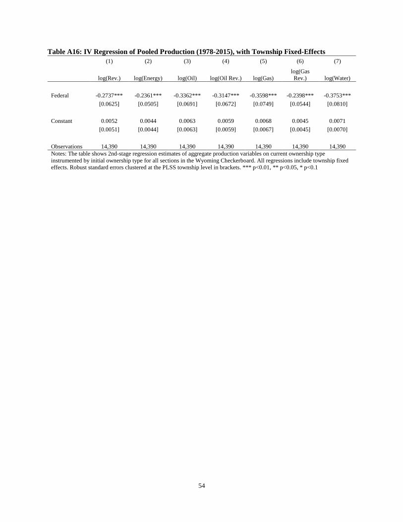
54

Table A16: IV Regression of Pooled Production (1978-2015), with Township Fixed-Effects (1) (2) (3) (4) (5) (6) (7)

log(Rev.) log(Energy) log(Oil) log(Oil Rev.) log(Gas) log(Gas Rev.) log(Water)

Federal -0.2737*** -0.2361*** -0.3362*** -0.3147*** -0.3598*** -0.2398*** -0.3753***

[0.0625] [0.0505] [0.0691] [0.0672] [0.0749] [0.0544] [0.0810]

Constant 0.0052 0.0044 0.0063 0.0059 0.0068 0.0045 0.0071

[0.0051] [0.0044] [0.0063] [0.0059] [0.0067] [0.0045] [0.0070]

Observations 14,390 14,390 14,390 14,390 14,390 14,390 14,390 Notes: The table shows 2nd-stage regression estimates of aggregate production variables on current ownership type instrumented by initial ownership type for all sections in the Wyoming Checkerboard. All regressions include township fixed effects. Robust standard errors clustered at the PLSS township level in brackets. *** p<0.01, ** p<0.05, * p<0.1

55

Table A17: IV Regression of Pooled Production (1978-2015), Conditional on Production with Township Fixed Effects

(1) (2) (3) (4) (5) (6) (7)

log(Rev.) log(Energy) log(Oil) log(Oil Rev.) log(Gas) log(Gas Rev.) log(Water)

Federal 0.1158 0.1384 -0.0019 -0.0010 0.0502 0.0372 0.1860

[0.0995] [0.1006] [0.1212] [0.1477] [0.1207] [0.1246] [0.1286]

Observations 1,773 1,773 1,773 1,773 1,773 1,773 1,773 Notes: The table shows 2nd-stage regression estimates of aggregate production variables on current ownership type instrumented by initial ownership type. All specifications include township fixed effects. Robust standard errors in brackets. *** p<0.01, ** p<0.05, * p<0.1

Table A18: IV Regression of Pooled Production (1978-2015), Conditional on Production with Firm Fixed Effects

(1) (2) (3) (4) (5) (6) (7)

log(Rev.) log(Energy) log(Oil) log(Oil Rev.) log(Gas) log(Gas Rev.) log(Water) Federal 0.2699* 0.2680* 0.2381 0.2963 0.3363** 0.3420** 0.2436

[0.1396] [0.1426] [0.2031] [0.2544] [0.1699] [0.1738] [0.1780]

Observations 1,773 1,773 1,773 1,773 1,773 1,773 1,773 Notes: The table shows 2nd-stage regression estimates of aggregate production variables on current ownership type instrumented by initial ownership type. All specifications include firm-specific fixed effects. Robust standard errors in brackets. *** p<0.01, ** p<0.05, * p<0.1

56

Table A19: Naïve Spill Analysis Results (1) (2) (3) (4) (5) (6)

VARIABLES Section Spilled

Section Spilled

Section Spilled

Section Spilled

Section Spilled

Section Spilled

Federal -0.0146*** -0.0139*** -0.0144*** -0.0143*** -0.0121*** -0.0131***

[0.0026] [0.0026] [0.0026] [0.0028] [0.0027] [0.0027] Per 1000 Wells 0.3879*** 0.4242***

[0.0928] [0.1074] Million BOE 0.0391 0.0647*

[0.0308] [0.0382]

Observations 26,237 26,237 26,237 26,237 26,237 26,237 Fixed Effects Year Year Year Year, Twsp Year, Twsp Year, Twsp Notes: The table shows OLS regression estimates of whether a section had a spill in a given year (1992-2015), conditional on the section being in production, on current ownership. Robust standard errors clustered at the PLSS township level in brackets. *** p<0.01, ** p<0.05, * p<0.1

Table A20: Naïve Spill Analysis Results with Firm Fixed Effects (1) (2) (3) (4) (5) (6)

VARIABLES Section Spilled

Section Spilled

Section Spilled

Section Spilled

Section Spilled

Section Spilled

Federal -

0.0129*** -0.0113*** -0.0125*** -0.0122*** -0.0090*** -0.0104*** [0.0029] [0.0027] [0.0029] [0.0028] [0.0026] [0.0026]

Per 1000 Wells 0.4321*** 0.4488***

[0.0936] [0.1151] Million BOE 37,780 74,170*

[32,579] [40,857] Observations 27,517 27,517 27,517 27,517 27,517 27,517

Fixed Effects Year, Firm Year, Firm Year, Firm Year, Twsp,

Firm Year, Twsp,

Firm Year, Twsp,

Firm Notes: The table shows OLS regression estimates of whether a section had a spill in a given year (1992-2015), conditional on the section being in production, on current ownership. All regressions include controls for firm fixed effects. Robust standard errors clustered at the PLSS township level in brackets. *** p<0.01, ** p<0.05, * p<0.1

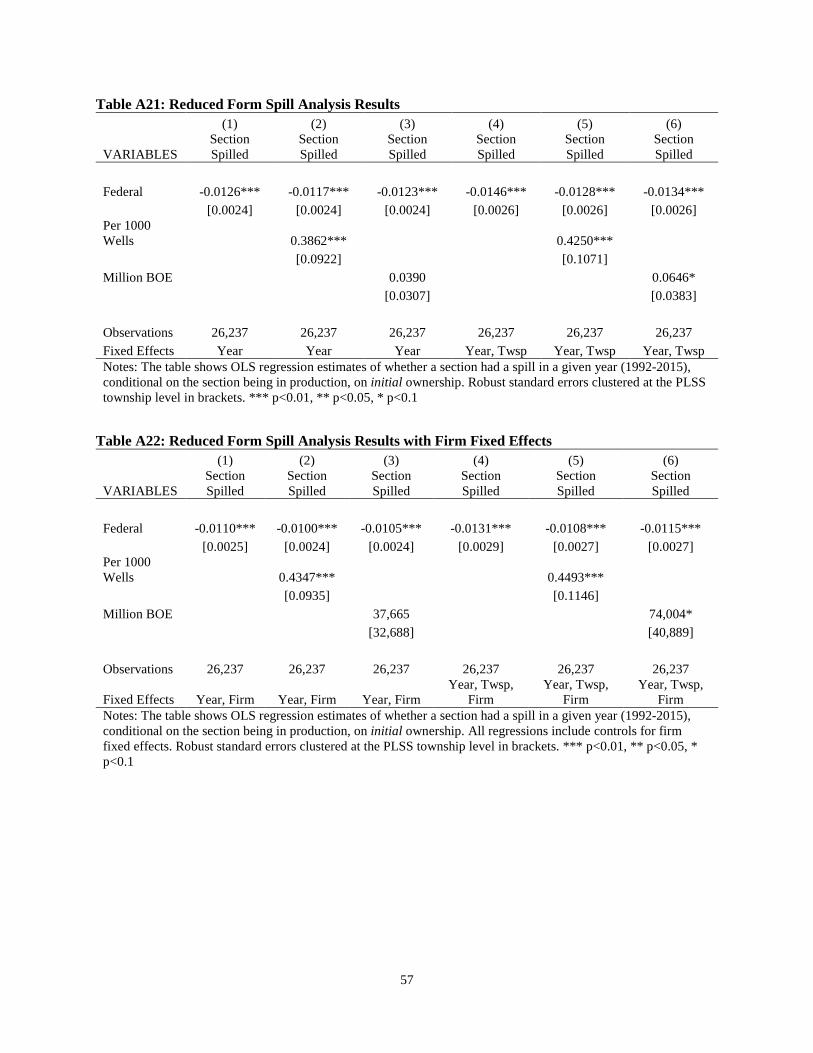
57

Table A21: Reduced Form Spill Analysis Results (1) (2) (3) (4) (5) (6)

VARIABLES Section Spilled

Section Spilled

Section Spilled

Section Spilled

Section Spilled

Section Spilled

Federal -0.0126*** -0.0117*** -0.0123*** -0.0146*** -0.0128*** -0.0134***

[0.0024] [0.0024] [0.0024] [0.0026] [0.0026] [0.0026] Per 1000 Wells 0.3862*** 0.4250***

[0.0922] [0.1071] Million BOE 0.0390 0.0646*

[0.0307] [0.0383] Observations 26,237 26,237 26,237 26,237 26,237 26,237 Fixed Effects Year Year Year Year, Twsp Year, Twsp Year, Twsp Notes: The table shows OLS regression estimates of whether a section had a spill in a given year (1992-2015), conditional on the section being in production, on initial ownership. Robust standard errors clustered at the PLSS township level in brackets. *** p<0.01, ** p<0.05, * p<0.1

Table A22: Reduced Form Spill Analysis Results with Firm Fixed Effects (1) (2) (3) (4) (5) (6)

VARIABLES Section Spilled

Section Spilled

Section Spilled

Section Spilled

Section Spilled

Section Spilled

Federal -0.0110*** -0.0100*** -0.0105*** -0.0131*** -0.0108*** -0.0115***

[0.0025] [0.0024] [0.0024] [0.0029] [0.0027] [0.0027] Per 1000 Wells 0.4347*** 0.4493***

[0.0935] [0.1146] Million BOE 37,665 74,004*

[32,688] [40,889]

Observations 26,237 26,237 26,237 26,237 26,237 26,237

Fixed Effects Year, Firm Year, Firm Year, Firm Year, Twsp,

Firm Year, Twsp,

Firm Year, Twsp,

Firm Notes: The table shows OLS regression estimates of whether a section had a spill in a given year (1992-2015), conditional on the section being in production, on initial ownership. All regressions include controls for firm fixed effects. Robust standard errors clustered at the PLSS township level in brackets. *** p<0.01, ** p<0.05, * p<0.1

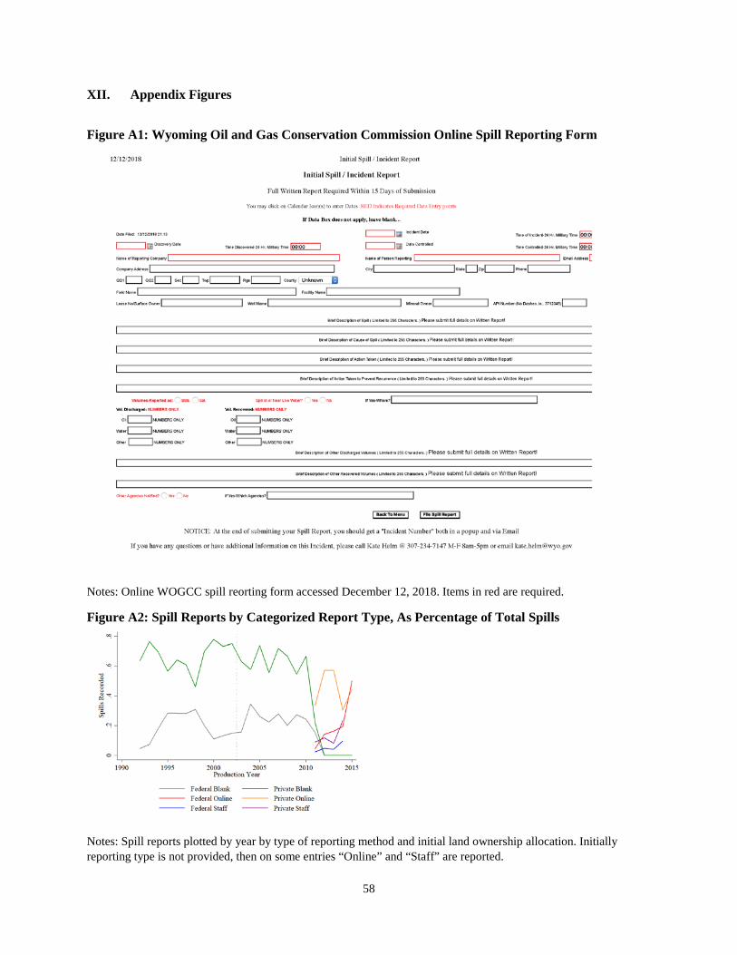
58

XII. Appendix Figures

Figure A1: Wyoming Oil and Gas Conservation Commission Online Spill Reporting Form

Notes: Online WOGCC spill reorting form accessed December 12, 2018. Items in red are required.

Figure A2: Spill Reports by Categorized Report Type, As Percentage of Total Spills

Notes: Spill reports plotted by year by type of reporting method and initial land ownership allocation. Initially reporting type is not provided, then on some entries “Online” and “Staff” are reported.

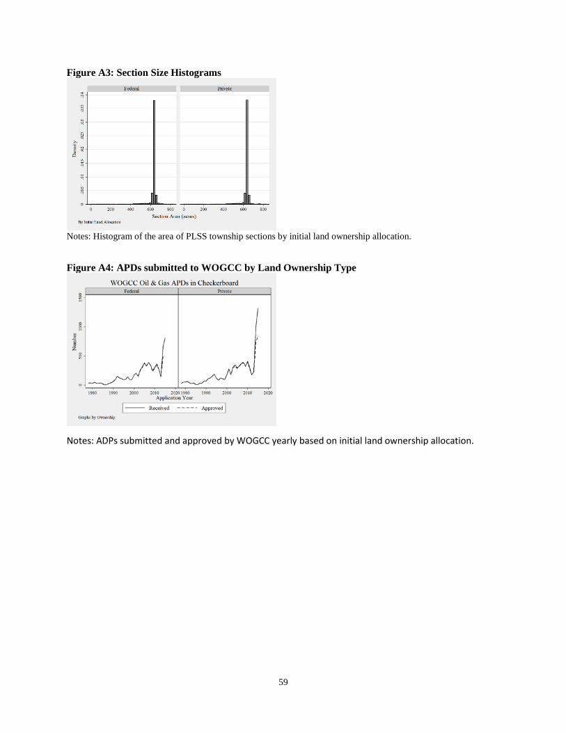
59

Figure A3: Section Size Histograms

Notes: Histogram of the area of PLSS township sections by initial land ownership allocation.

Figure A4: APDs submitted to WOGCC by Land Ownership Type

Notes: ADPs submitted and approved by WOGCC yearly based on initial land ownership allocation.

60

Figure A5: APDs submitted to WOGCC by Associated BLM Field Office Region A B

Notes: Panel A shows ADPs received and approved by WOGCC by year based on the location of the section in each of the BLM field office jurisdictions (current jurisdictions for all years) for al level application types. Panel B shows the types of permits received by field office over time.

Figure A6: Median Time from Spud to Completion

Notes: Median time from well spud to completion in days conditional on initial land assignment.

010

020

030

0M

edia

n Ti

me

from

Spu

d to

Com

plet

ion

(day

s)

1980 1990 2000 2010 2020Permit Approval Year

Federal Private

61

Figure A7: Expired Permits per Proposed Well

Notes: Mean number of expired WOGCC permit (duraction one-year) for a given well, conditional on initial allocation of land. Numbers>1 indicated a permit has expired and been renewed, then expired again.

Figure A8: Proportion of Permits Never Drilled

Notes: Proportion of permits approved in a given year that have not been drilled as of 2015, conitional on lan allocation.

0.5

11.

5Ex

pire

d pe

rmits

per

API

1980 1990 2000 2010 2020Permit Approval Year

Federal Private

Expired Permits0

.2.4

.6.8

prop

ortio

n of

app

rove

d pe

rmits

with

no

spud

1980 1990 2000 2010 2020Permit Approval Year

Federal Private

Permit Approved but Well Not Drilled

62

Figure A9: Permit Approvals/Renewals per Proposed Well

Notes: Mean number of times a well has renewed its WOGCC permit (duraction one-year), conditional on initial allocation of land. Numbers>1 indicated a permit has expired and been renewed, then expired again.

11.

21.

41.

61.

8Pe

rmit

Appr

oval

s/R

enew

als

per P

ropo

sed

Wel

l

1980 1985 1990 1995 2000 2005 2010 2015Initial Permit Approval Year

Federal Private