SOME THOUGHTS ABOUT THE DESIGN OF LOSS FUNCTIONS - INE · 2007-03-13 · Some Thoughts About the Design of Loss Functions 21 1. INTRODUCTION Most statistical problems are deﬁned

REVSTAT – Statistical Journal

Volume 5, Number 1, March 2007, 19–39

SOME THOUGHTS ABOUT THE DESIGN OF

LOSS FUNCTIONS

Authors: Christian Hennig

– Department of Statistical Science,University College London,United [email protected]

Mahmut Kutlukaya

– Strategy Development Department,Banking Regulation and Supervision Agency,Kavaklidere-Ankara, [email protected]

Abstract:

• The choice and design of loss functions is discussed. Particularly when computationalmethods like cross-validation are applied, there is no need to stick to “standard”loss functions such as the L2-loss (squared loss). Our main message is that the choiceof a loss function in a practical situation is the translation of an informal aimor interest that a researcher may have into the formal language of mathematics.The choice of a loss function cannot be formalized as a solution of a mathematicaldecision problem in itself. An illustrative case study about the location of branchesof a chain of restaurants is given. Statistical aspects of loss functions are treated,such as the distinction between applications of loss functions to prediction and esti-mation problems and the direct definition of estimators to minimize loss functions.The impact of subjective decisions to the design of loss functions is also emphasizedand discussed.

Key-Words:

• prediction; estimation; decision theory; M-estimator; MM-estimator; linear regression.

AMS Subject Classification:

• 62A01, 62C05, 62G09, 62J05, 62M20.

20 Christian Hennig and Mahmut Kutlukaya

Some Thoughts About the Design of Loss Functions 21

1. INTRODUCTION

Most statistical problems are defined in terms of loss functions in the sense

that loss functions define what a “good” estimator or a “good” prediction is.

This paper discusses some aspects of the choice of a loss function. The main

message of the paper is that the task of choosing a loss function is about the

translation of an informal aim or interest that a researcher may have in the given

application into the formal language of mathematics. The choice of a loss function

cannot be formalized as a solution of a mathematical decision problem in itself,

because such a decision problem would require the specification of another loss

function. Therefore, the choice of a loss function requires informal decisions,

which necessarily have to be subjective, or at least contain subjective elements.

This seems to be acknowledged somewhat implicitly in the decision theoretic

literature, but we are not aware of any sources where this is discussed in detail.

Several different uses of loss functions can be distinguished.

(a) In prediction problems, a loss function depending on predicted and

observed value defines the quality of a prediction.

(b) In estimation problems, a loss function depending on the true pa-

rameter and the estimated value defines the quality of estimation.

As opposed to prediction problems, this assumes a statistical model

to hold, which defines the parameter to be estimated. The true param-

eter value in an estimation problem is generally unobservable, while

in a prediction problem the “truth” is observable in the future.

(c) Definition of estimators: many estimators (such as least squares or

M-estimators) are defined as optimizers of certain loss functions which

then depend on the data and the estimated value. Note that this

is essentially different from (a) and (b) in the sense that the least

squares estimator is not necessarily the estimator minimizing the

mean squared estimation error or the squared prediction error.

There are several further uses of loss functions, which won’t be treated in

the present paper, for instance defining optimal testing procedures, Bayesian risk,

etc.

While general loss functions have been treated in the literature1, versions of

the squared loss function are used in a vast majority of applications of prediction

and estimation problems (note that UMVU estimation is a restricted optimization

of a squared loss function). Main reasons for this seem to be the simplicity of

the mathematics of squared loss and the self-confirming nature of the frequent

1See, for instance, Lehmann and Casella ([6]), who mainly use squared loss, but discussalternatives in several chapters.


use of certain “standard” methods in science. However, if prediction methods are

compared using nonparametric resampling techniques such as cross-validation

and bootstrap, there is no computational reason to stick to the squared loss, and

other loss functions can be used. Robustness aspects of loss functions have been

discussed previously by Ronchetti, Field and Blanchard ([9]) and Leung ([7]).

In Section 2, the subject-matter dependent design of a loss function in

a business application using robust regression is discussed to give an illustrating

example of the “translation problem” mentioned above and to motivate some of

the discussion in the following sections.

In Section 3, the implications of the different statistical uses of loss func-

tions (a), (b) and (c) above are explored in more detail. The question whether

the negative loglikelihood can be considered as the “true” objective loss function

in estimation is discussed.

In Section 4, some philosophical aspects are treated. In particular, the con-

cepts of subjectivity and objectivity, emphasizing the role of subjective decisions

in the choice of loss functions, and the standardizing role of communication in

the scientific community are discussed. Finally, a brief conclusion is given.

2. LOCATIONS OF RESTAURANTS: A CASE STUDY

The case study presented in this section is about a prediction problem

in a business application. Because the original study is confidential, the story

presented here is made up, and the original data are not shown. The values and

rankings in Tables 1 and 2, however, are authentic (absolute and squared losses

have been multiplied by a constant).

A restaurant chain wanted to predict the turnover for new branches,

depending on the following six independent variables:

• number of people living in a (suitably defined) neighborhood,

• number of people working or shopping at daytime in the neighborhood,

• number of branches of competitors in the neighborhood,

• size of the branch,

• a wealth indicator of the neighborhood,

• distance to the next branch of the same chain.

The results are to be used to support decisions such as where to open new

branches, and what amount of rents or building prices can be accepted for par-

ticular locations. Data from 154 already existing branches on all the variables


were available. In our study we confined ourselves to finding a good linear regres-

sion type prediction rule, partly because the company wanted to have a simple

formula, and partly because an alternative (regression trees) had already been

explored in a former project.

The data are neither apparently nonlinear, nor heteroscedastic in any clear

systematic way. However, there are obvious outliers. We decided to choose the

best out of several more or less robust linear regression estimators using leave-

one-out cross-validation (LOO-CV). In the real study, choice of transformations

of variables and variable selection have also been considered, but this doesn’t add

to the discussion of interest here.

Note that LOO-CV processes all data points in the same manner, which

means that all observations are treated as if they were a representative sample

from the underlying population of interest. Particularly, outliers are treated in

the same way as seemingly more typical data points (but may be weighted down

implicitly, see below). This makes sense if there is no further subject matter

information indicating that the outliers are erroneous or atypical in a way that

we would not expect similar observations anymore in the future. In the given

case study, outlying observations are not erroneous and stem from restaurants at

some locations with special features. It may well be possible that further outliers

occur in the future for similar reasons.

The estimators we took into account were

• the least squares (LS)-estimator,

• the least median of squares (LMS)-estimator as suggested by Rousseeuw

([10]),

• Huber’s M-estimator for linear regression with tuning constant k=1.345

to produce 95% efficiency for normal samples, see Huber ([5]),

• an M-estimator for linear regression using the “bisquared” objective

function with tuning constant k = 4.685 to produce 95% efficiency for

normal samples, see Western ([13]),

• the MM-estimator suggested by Yohai ([14]) tuned to 95% efficiency

for normal samples.

In principle, it is reasonable to include M-/MM-estimators tuned to smaller effi-

ciency as well, which will then potentially downweight some further outliers.

However, we compared several tunings of the MM-estimator in one particular

situation, from which we concluded that not too much gain is to be expected

from smaller tunings than 95% efficiency (larger efficiencies can be better, but

our results on this are quite unstable).

All estimators were used as implemented in R (www.R-project.org), but

the implementations we used for this project have been replaced by new ones


in the meantime (in packages “MASS” and “robustbase”). The scale estimator

used for the two M-estimators was a re-scaled median absolute deviance (MAD)

based on the residuals (as implemented in the function rlm).

The estimators have been compared according to the estimated expected

prediction error

(2.1)1

n

n∑

i=1

L(yi, y−i) ,

where n is the number of observations, y1, ..., yn are the observed turnovers, and

y−i is the predicted value of the turnover for yi from applying the linear regression

method to the data omitting the i th observation. L is a loss function, of which

the design will be discussed in the following.

Note that (2.1) already implies some decisions. Firstly, L is defined here

to depend on yi and y−i only, but not directly on the values of the independent

variables of the i th observation. In general, this restriction is not required, but

it is justified in the present setup by the fact that the company didn’t specify

any particular dependence of their tolerance of prediction errors on the values of

the independent variables, and there is no obvious subject-matter reason in the

present study for such a dependence to be needed. This is a first illustration of

our major principle to translate the informal interests and aims of those who use

the results in the formal mathematical language.

Secondly, it is part of the design of the loss function not just to choose L,

but also to decide about how the values of L(yi, y−i) should be aggregated.

Their mean is used in (2.1), but instead, their maximum, their median, another

quantile or a trimmed mean could be chosen as well. Note that there is some

interaction between the choice of L and the choice of how the values of L are

to be aggregated. For example, under the assumption that we would like to do

something robust against outliers, the choice of a bounded L-function bounds the

influence of extreme prediction errors in itself and allows therefore the aggrega-

tion of the L-values in a less robust manner such as taking their mean. For the

present study, we confine ourselves to the mean, of which the interpretation is

that the prediction error of every single observation is judged as equally impor-

tant to us, and we will deal with the influence of extreme observations via the

choice of L.

As mentioned before, the “standard” loss function for this kind of prob-

lem is defined by L2(y, y) = (y − y)2, but because we use LOO-CV, there is

no mathematical reason to use L = L2.

One of the decisions to make is whether L should be symmetric. This means

that a negative prediction error is judged as causing the same loss as a positive

error of the same absolute value. This is difficult to judge in the present situation.


It could be argued that it is not as bad for the company to underestimate the

turnover at a particular location than to overestimate it, because the money spent

by the company on a branch with overestimated turnover may be lost.

However, because the prediction should guide the decision whether a branch

should be opened in the first place, how much rent should be paid and also

how the branch will be initially equipped, underestimation of the turnover may

have serious consequences as well, as offers for good locations may be turned

down or under-equipped. Though the effects of over- and underestimation can

be considered to be asymmetric in the present setup, we decided to stick to

symmetric loss functions, meaning that the loss of paid money is treated as equally

bad as the loss of money which is not earned because of a missed opportunity.

A main feature of L2 is its convexity, which means that the differences

between high prediction errors are assessed as more important than differences

between small prediction errors. As an example, consider two prediction rules

that only differ with respect to their cross-validated predictions of two data points,

y1 and y2. Suppose that for rule 1, y1−y−1 =10,000, y2−y−2 =−10, and for rule 2,

y1− y−1 = 9,990, y2− y−2 =−20 (the units of y don’t have a particular meaning

here because we have to use artificial values anyway, but you may imagine them

to mean £ 1,000 a year). L2 favours rule 2 in this situation. But is this adequate?

Going back to the discussion above, if the values could be interpreted as

earned (or lost) money, the L1-loss (L1(y, y) = |y− y|) seemed to be more ade-

quate, because it assesses both rules as equally good, based on the fact that they

both cause the same direct or indirect financial loss of 10,010 units. For the

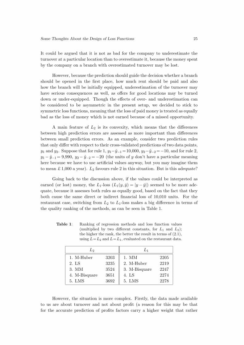
restaurant case, switching from L2 to L1-loss makes a big difference in terms of

the quality ranking of the methods, as can be seen in Table 1.

Table 1: Ranking of regression methods and loss function values(multiplied by two different constants, for L1 and L2);the higher the rank, the better the result in terms of (2.1),using L=L2 and L=L1, evaluated on the restaurant data.

L2 L1

1. M-Huber 3203 1. MM 2205

2. LS 3235 2. M-Huber 2219

3. MM 3524 3. M-Bisquare 2247

4. M-Bisquare 3651 4. LS 2274

5. LMS 3692 5. LMS 2278

However, the situation is more complex. Firstly, the data made available

to us are about turnover and not about profit (a reason for this may be that

for the accurate prediction of profits factors carry a higher weight that rather


have to do with management decisions than with the location of the branch).

Usually, profits are less sensitive against differences between two large values of

turnovers than against the same absolute differences between two smaller values

of turnovers. Therefore, more tolerance is allowed in the prediction of larger

yi-values.

Secondly, the data give turnovers over a long period (three years, say),

and after a new branch has been opened, if it turns out after some months that

the turnover has been hugely wrongly predicted, the management has several

possibilities of reaction, ranging from hiring or firing staff over special offers and

campaigns attracting more customers to closing the branch.

Therefore, if predictions are hugely wrong, it matters that they are hugely

wrong, but it doesn’t matter too much how wrong they exactly are. This means

that, at least for large absolute errors, the loss function should be concave if not

constant. Actually we chose a function which is constant for large absolute errors,

because we could give the lowest absolute error above which the loss function is

constant a simple interpretation: above this error value, predictions are treated

as “essentially useless” and it doesn’t matter how wrong they precisely are. This

interpretation could be communicated to the company, and the company was

then able to specify this limiting value. The design of a concave but strictly

increasing function would have involved much more complicated communication.

The company initially specified the critical value for “usefulness” as 10% of

the true turnover, i.e., they were concerned about relative rather than absolute

error, which motivated the following loss function:

Lc(y, y) =

(y− y)2

y2:

(y− y)2

y2≤ c2

c2 :(y− y)2

y2> c2 ,

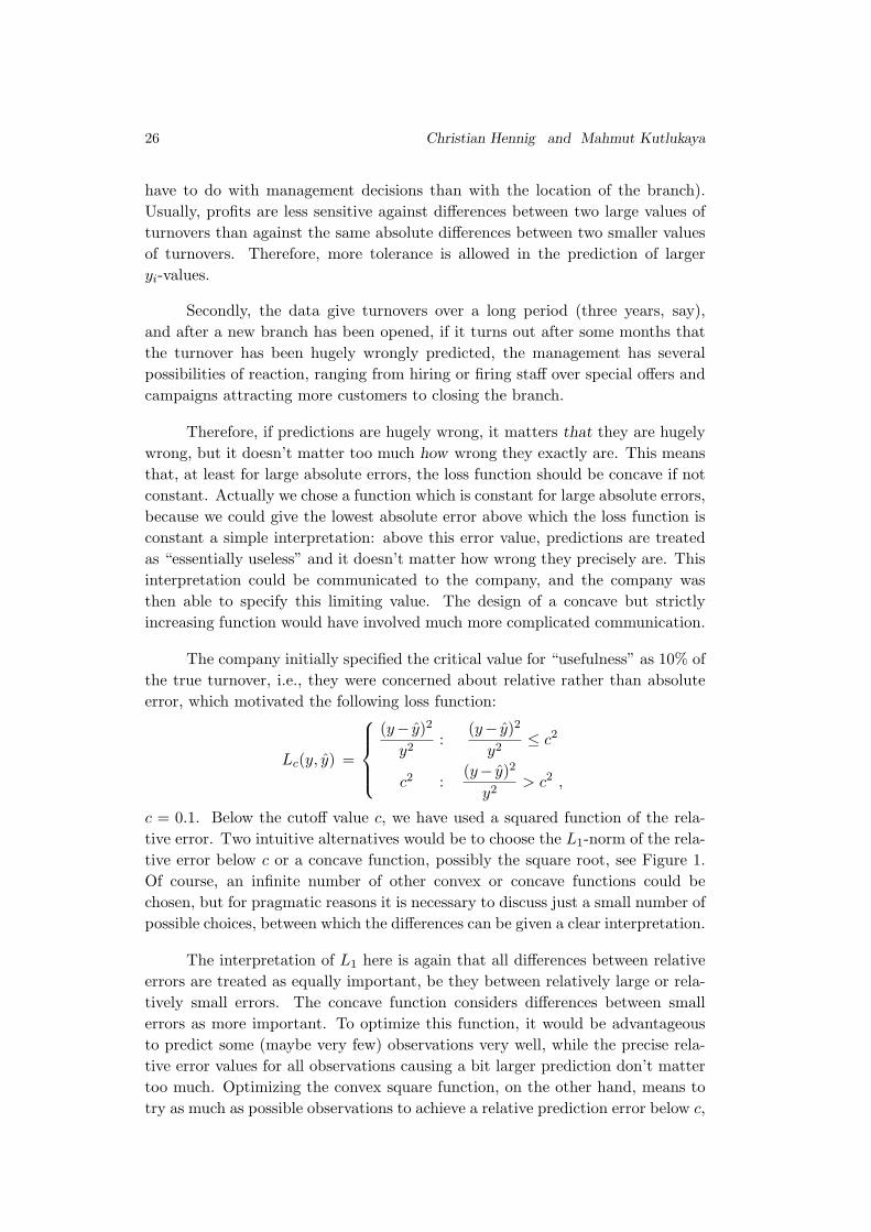
c = 0.1. Below the cutoff value c, we have used a squared function of the rela-

tive error. Two intuitive alternatives would be to choose the L1-norm of the rela-

tive error below c or a concave function, possibly the square root, see Figure 1.

Of course, an infinite number of other convex or concave functions could be

chosen, but for pragmatic reasons it is necessary to discuss just a small number of

possible choices, between which the differences can be given a clear interpretation.

The interpretation of L1 here is again that all differences between relative

errors are treated as equally important, be they between relatively large or rela-

tively small errors. The concave function considers differences between small

errors as more important. To optimize this function, it would be advantageous

to predict some (maybe very few) observations very well, while the precise rela-

tive error values for all observations causing a bit larger prediction don’t matter

too much. Optimizing the convex square function, on the other hand, means to

try as much as possible observations to achieve a relative prediction error below c,


while differences between small errors don’t have a large influence. Because the

company is interested in useful information about many branches, rather than

to predict few branches very precisely, we chose the squared function below c.

0.00 0.05 0.10 0.15

0.00

0.05

0.10

0.15

r

l(r)

Figure 1: Bounded functions of the relative prediction error r,the lower part being squared, L1 and square root.

Unfortunately, when we carried out the comparison, it turned out that

the company had been quite optimistic about the possible quality of prediction.

Table 2 (left side) shows the ranking of the estimators, but also the number

of observations of which the relative prediction error has been smaller than c,

i.e., for which the prediction has not been classified as “essentially useless”.

Table 2: Ranking and loss function values of regression methodsin terms of (2.1), using L = Lc with c = 0.1 and c = 0.2.The number of observations of which the prediction hasnot been classified as “essentially useless” is also given.

Ranking # obs. 107∗ Ranking # obs. 106∗c = 0.1 (y−y)2

y2 ≤ 0.12 L0.1 c = 0.2 (y−y)2

y2 ≤ 0.22 L0.2

1. M-Huber 42 8117 1. MM 85 2474

2. M-Bisquare 49 8184 2. M-Bisquare 86 2482

3. LS 38 8184 3. M-Huber 83 2494

4. MM 49 8195 4. LMS 75 2593

5. LMS 39 8373 5. LS 81 2602


With n = 154, this is less than a third of the observations for all methods.

Confronted with this, the company decided to allow relative prediction errors

up to 20% to be called “useful”, which at least made it possible to obtain reason-

able predictions for more than half of the observations. The company accepted

this result (which can be seen on the right side of Table 2) though we believe

that accepting even larger relative errors for more branches as “useful” would

be reasonable, given the precision of the data at hand. One could also think

about using a squared function of the relative error below c = 0.2, constant loss

above c = 0.4 and something concave in between, which, however, would have

been difficult to negotiate with the company. The question whether it would be

advantageous to use an estimator that directly minimizes∑

L(y, y), given a loss

function L, instead of comparing other estimators in terms of L is treated in

Section 3.1.

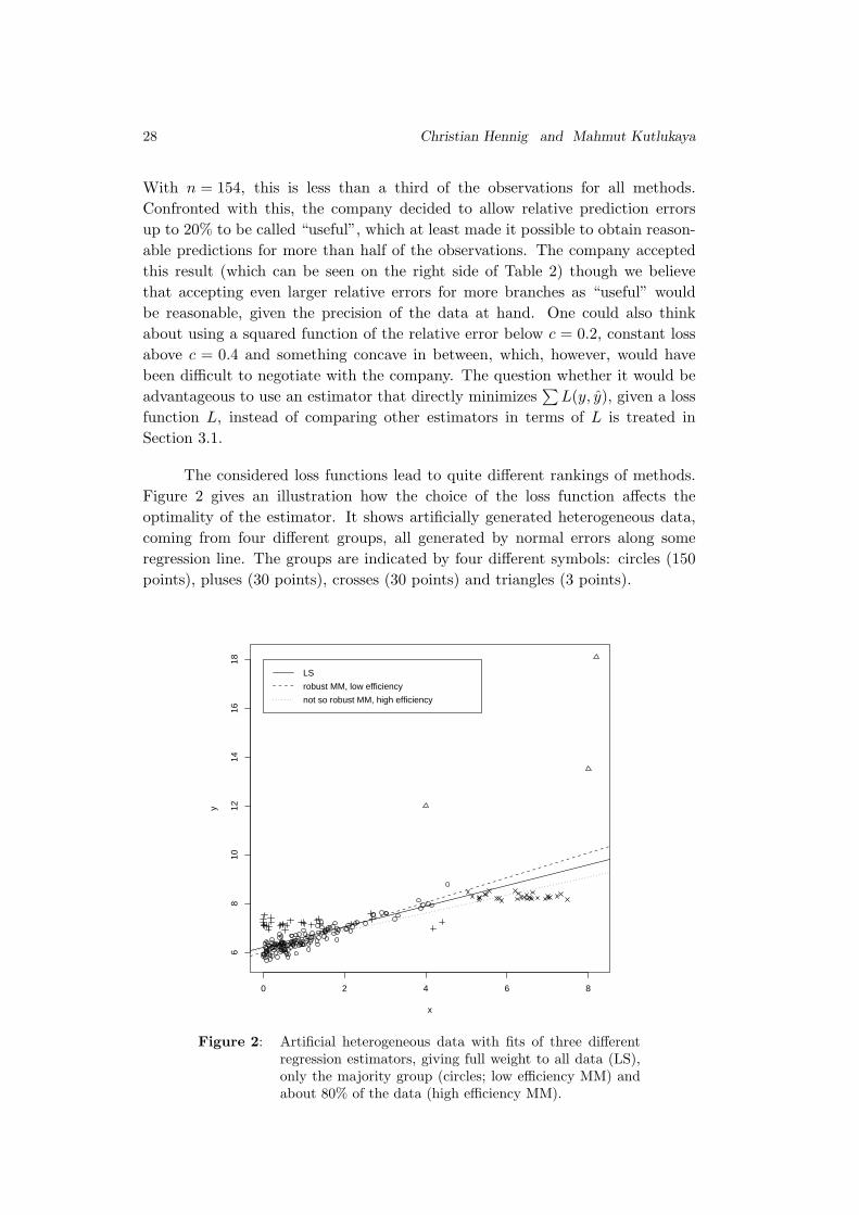
The considered loss functions lead to quite different rankings of methods.

Figure 2 gives an illustration how the choice of the loss function affects the

optimality of the estimator. It shows artificially generated heterogeneous data,

coming from four different groups, all generated by normal errors along some

regression line. The groups are indicated by four different symbols: circles (150

points), pluses (30 points), crosses (30 points) and triangles (3 points).

0 2 4 6 8

68

1012

1416

18

x

y

LS

robust MM, low efficiency

not so robust MM, high efficiency

Figure 2: Artificial heterogeneous data with fits of three differentregression estimators, giving full weight to all data (LS),only the majority group (circles; low efficiency MM) andabout 80% of the data (high efficiency MM).


The plot has a rough similarity with some of the scatterplots from the original

restaurants data. If the aim is to fit some points very well, and the loss function

is chosen accordingly, the most robust “low efficiency MM-estimator” in Figure 2

is the method of choice, which does the best job for the majority of the data.

A squared loss function would emphasize to make the prediction errors for the

outlying points (triangles) as small as possible, which would presumably favour

the LS-estimator here (this is not always the case, see Section 3). However, if

the aim is to yield a good relative prediction error for more data than fitted well

by the robust estimator, the less robust, but more efficient MM-estimator (or an

estimator with breakdown point of, say, 75%) leads to a fit that does a reasonable

job for circles, crosses, and some of the pluses. The decision about the best ap-

proach here is depending on the application. For instance, an insurance company

may be interested particularly in large outliers and will choose a different loss

function from a company which considers large prediction errors as “essentially

useless”. But even such a company may not be satisfied by getting only a tight

majority of the points about right.

3. STATISTICAL ASPECTS

Though Section 2 was about prediction, methods have been compared that

were originally introduced as parameter estimators for certain models, and that

are defined via optimizing some objective (loss) functions. Therefore the applica-

tions (a), (b) and (c) of loss functions mentioned in the introduction were involved.

Here are some remarks about differences and relations between these uses.

3.1. Prediction loss vs. objective functions defining estimators

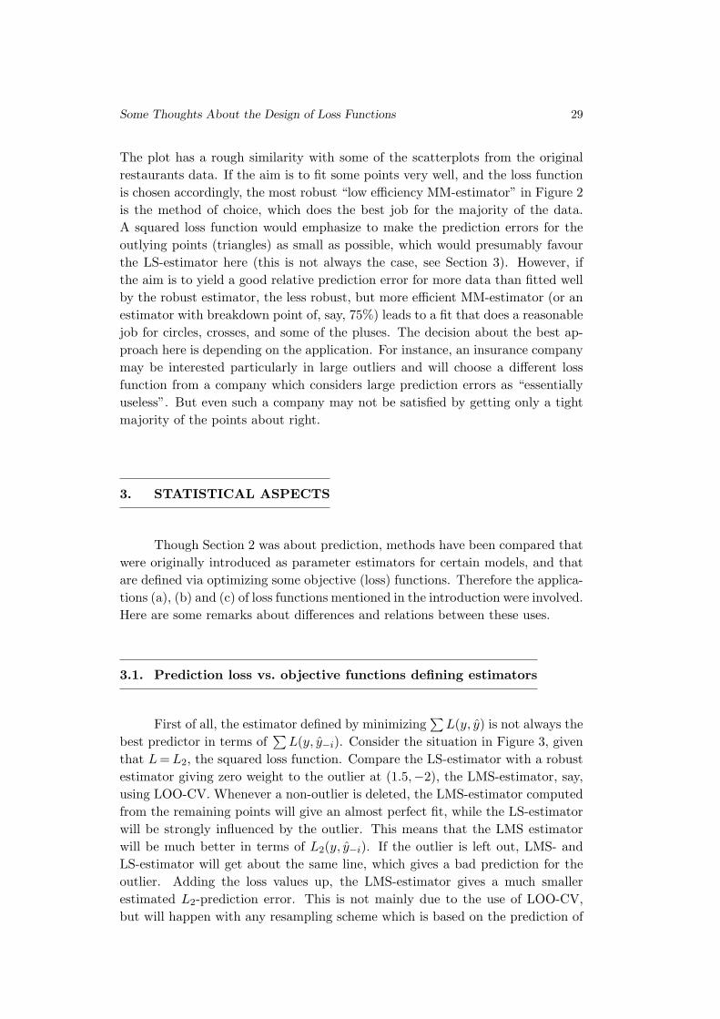
First of all, the estimator defined by minimizing∑

L(y, y) is not always the

best predictor in terms of∑

L(y, y−i). Consider the situation in Figure 3, given

that L = L2, the squared loss function. Compare the LS-estimator with a robust

estimator giving zero weight to the outlier at (1.5,−2), the LMS-estimator, say,

using LOO-CV. Whenever a non-outlier is deleted, the LMS-estimator computed

from the remaining points will give an almost perfect fit, while the LS-estimator

will be strongly influenced by the outlier. This means that the LMS estimator

will be much better in terms of L2(y, y−i). If the outlier is left out, LMS- and

LS-estimator will get about the same line, which gives a bad prediction for the

outlier. Adding the loss values up, the LMS-estimator gives a much smaller

estimated L2-prediction error. This is not mainly due to the use of LOO-CV,

but will happen with any resampling scheme which is based on the prediction of


a subsample of points by use of the remaining points. The situation changes (for

LOO-CV) when further outliers are added at about (−1.5, 2). In this case, the

LS-estimator is better in terms of the estimated L2-prediction error, because this

is dominated by the outliers, and if one outlier is left out, the further outliers

at about the same place enable LS to do a better job on these than the robust

estimator. The situation is again different when outliers are added at other

locations in a way that none of the outliers provides useful information to predict

the others. In this situation, it depends strongly on where exactly the outliers

are whether LOO-CV prefers LS or LMS. Here, the assessment of the prediction

error itself is non-robust and quite sensitive to small changes in the data.

−1.0 −0.5 0.0 0.5 1.0 1.5

−12

−10

−8

−6

−4

−2

x

y

LS

LMS

Figure 3: Artificial data with fits of LS and LMS estimator.

From a theoretical point of view, apart from the particular use of LOO-CV

to estimate the prediction error, LS is clearly better than LMS in terms of

L2-prediction loss, in a “normal model plus outliers” situation, if the outliers

make it possible to find a suitable compromise between fitting them and the

majority, while it is bad for LS if the outliers are scattered all over the place

and one outlier doesn’t give useful information about the prediction of the others

(as for example in a linear model with Cauchy random term). Whether the

L2-loss is reasonable or the LMS-fit should be preferred because it predicts the

“good” majority of the data better even in cases where the outliers can be used

to predict each other depends on subject-matter decisions.


Asymptotically, using empirical process theory, it is often possible to show

that the estimator defined by minimizing∑

L(y, y) is consistent for θ minimizing

EL(y, θ) (in such situations, optimal prediction optimizing L and estimation of θ

are equivalent). Therefore, for a given loss function, it makes at least some sense

to use the estimator defined by the same objective function. However, this is

often not optimal, not even asymptotically, as will be shown in the next section.

3.2. Prediction and maximum likelihood-estimation

Suppose that the data have been generated by some parametric model.

Then there are two different approaches to prediction:

1. find a good prediction method directly, or

2. estimate the true model first, as well as possible, solve the prediction

problem theoretically on the model and then plug in the estimated

parameter into the theoretical prediction rule.

As an example, consider i.i.d. samples from an exponential(λ)-distribution, and

consider prediction optimizing L1-loss. The sample median suggests itself as a

prediction rule, minimizing∑

L1(y− y). The theoretical median (and therefore

the asymptotically optimal prediction rule) of the exponential(λ)-distribution is

log 2/λ, and this can be estimated by maximum likelihood as log 2/Xn, Xn being

the arithmetic mean. We have simulated 10,000 samples with n = 20 observations

from an exponential(1)-distribution. The MSE of the sample median has been

0.566 and the MSE of the ML-median has been 0.559. This doesn’t seem to be

a big difference, but using the paired Mann-Whitney test (not assuming a par-

ticular loss function), the advantage of the ML-median is highly significant with

p < 10−5, and the ML-median was better than the sample median in 6,098

out of 10,000 simulations.

Therefore, in this situation, it is advantageous to estimate the underlying

model first, and to derive predictions from the estimator. There is an asymptotic

justification for this, called the “convolution theorem” (see, e.g., Bickel et al, [1],

p. 24). A corollary of it says that under several assumptions

(3.1) lim infn→∞

Eθ L(√

n(

Tn− q(θ))

)

≥ Eθ L(

Mn− q(θ))

,

where q(θ) is the parameter to be estimated (which determines the asymptoti-

cally optimal prediction rule), Tn is an estimator and Mn is the ML-estimator.

This holds for every loss function L which is a function of the difference between

estimated and true parameter satisfying

(3.2) L(x) = L(−x) ,{

x : L(x) ≤ c}

convex ∀ c > 0 .


(3.2) is somewhat restrictive, but not strongly so. For example, it includes all

loss functions discussed in Section 2 (applied to the estimation problem of the

optimal prediction rule instead of direct prediction, however).

This fact may provoke three misinterpretations:

1. estimation is essentially equivalent to prediction (at least asymptoti-

cally — though the exponential example shows that the implications

may already hold for small n),

2. the negative loglikelihood can be seen as the “true” loss function be-

longing to a particular model. In this sense the choice of the loss func-

tion would rather be guided by knowledge about the underlying truth

than by subjective subject-matter dependent decisions as illustrated in

Section 2,

3. all loss functions fulfilling (3.2) are asymptotically equivalent.

Our view is different.

1. The main assumption behind the convolution theorem is that we know

the true parametric model, which is obviously not true in practice.

While the ML-median performed better in our simulation, prediction

by log 2/Xn can be quite bad in terms of L1-loss if the true distribution

is not the exponential. The sample median can be expected to perform

well over a wide range of distributions (which can be backed up by

asymptotic theory, see above), and other prediction rules can turn out

to be even better in some situations using LOO-CV and the like,

for which we don’t need any parametric assumption.

The basic difference between prediction and estimation is that the truth

is observable in prediction problems, while it is not in estimation prob-

lems. In reality, it can not even be assumed that any probability model

involving an i.i.d. component holds. In such a case, estimation problems

are not well defined, while prediction problems are, and there are pre-

diction methods that are not based on any such model. Such methods

can be assessed by resampling methods as well (though LOO-CV admit-

tedly makes the implicit assumption that the data are exchangeable).

Apart from this, there are parametric situations, in which the as-

sumptions of the convolution theorem are not satisfied and optimal

estimation and optimal prediction are even asymptotically different.

For example, in many model selection problems, the BIC estimates

the order of a model consistently, as opposed to the AIC (Nishii [8]).

But often, the AIC can be proved to be asymptotically better for predic-

tion, because for this task underestimation of the model order matters

more than overestimation (Shibata [11], [12]).


2. The idea that the negative loglikelihood can be seen as the “true” loss

function belonging to a particular model (with which we have been

confronted in private communication) is a confusion of the different

applications of loss functions. The negative loglikelihood defines the

ML estimator, which is, according to the convolution theorem, asymp-

totically optimal with respect to several loss functions specifying an

estimation problem. These loss functions are assumed to be symmetric.

In some applications asymmetric loss functions may be justified, for

which different estimators may be optimal (for example shrinked or in-

flated ML-estimators; this would be the case in Section 2 if the company

had a rather conservative attitude, were less keen on risking money

by opening new branches and would rather miss opportunities as long

as they are not obviously excellent). This may particularly hold under

asymmetric distributions, for which not even the negative loglikelihood

itself is symmetric. (The idea of basing the loss function on the under-

lying distribution, however, could make some sense, see Section 3.4.)

In the above mentioned simulation with the exponential distribution,

LOO-CV with the L1-loss function decided in 6,617 out of 10,000 cases

that the ML-median is a better predictor than the sample median.

This shows that in a situation where the negative loglikelihood is a

good loss function to define a predictor, LOO-CV based on the loss

function in which we are really interested is able to tell us quite relia-

bly that ML is better than the predictor based on direct optimization

of this loss function (which is the sample median for L1).

3. The idea that all loss functions are asymptotically equivalent again only

applies to an estimation problem of a given parameter assuming that

the model is known. The convolution theorem doesn’t tell us in which

parameter q(θ) in (3.1) we should be interested. The L1-loss for the

prediction problem determines that it is the median.

3.3. Various interpretations of loss functions

According to our main hypothesis, the choice of a loss function is a trans-

lation problem. An informal judgment of a situation has to be translated into

a mathematical formula. To do this, it is essential to keep in mind how loss

functions are to be interpreted. This depends essentially on the use of the loss

function, referring to (a), (b) and (c) in the introduction.

(a) In prediction problems, the loss function is about how we measure the

quality of a predicted value, having in mind that a true value exists

and will be observable in the future. As can be seen from the restau-


rant example, this is not necessarily true, because if a prediction turns

out to be very bad early, the company will react, which prevents the

“true value” under the prediction model from being observed (it may

further happen that the very fact that the company selects locations

based on a new prediction method changes the underlying distribu-

tion). However, the idea of an observable true value to be predicted,

enables a very direct interpretation of the loss function in terms of

observable quantities.

(b) The situation is different in estimation problems, where the loss func-

tion is a function of an estimator and an underlying, essentially

unobservable quantity. The quantification of loss is more abstract

in such a situation. For example, the argument used in Section 2

to justify the boundedness of the loss function was that if the predic-

tion is so wrong that it is essentially useless, it doesn’t matter anymore

how wrong it exactly is. Now imagine the estimation of a treatment

effect in medicine. It may be that after some study to estimate the

treatment effect, the treatment is applied regularly to patients with

a particular disease. Even though, in terms of the prediction of the

effect of the treatment on one particular patient, it may hold that

it doesn’t matter how wrong a grossly wrong prediction exactly is,

the situation for the estimation of the overall effect may be much

different. Under- or overestimation of the general treatment effect

matters to quite a lot of patients, and it may be of vital importance

to keep the estimation error as small as possible in case of a not very

good estimation, while small estimation errors could easily be toler-

ated. In such a case, something like the L2-loss could be adequate for

estimation, while a concave loss is preferred for pointwise prediction.

It could be argued that, at least in some situations, the estimation

loss is nothing else than an accumulated prediction loss. This idea

may justify the choice of the mean (which is sensitive to large values)

to summarize more robust pointwise prediction losses, as in (2.1).

Note that the convolution theorem compares expected values of losses,

and the expectation as a functional is in itself connected to the L2-loss.

Of course, all of this depends strongly on the subject matter.

(c) There is also a direct interpretation that can be given to the use of

loss functions to define methods. This is about measuring the quality

of data summary by the method. For example, the L2-loss function

defining the least squares estimator defines how the locations of the

already observed data points are summarized by the regression line.

Because L2 is convex, it is emphasized that points far away from a

bulk of the data are fitted relatively well, to the price that most points

are not fitted as precisely as would be possible. Again, a decision has

to be made whether this is desired.


As a practical example, consider a clustering problem where a

company wants to assign k storerooms in order to deliver goods to

n shops so that the total delivery distance is minimized. This is an

L1-optimization problem (leading to k-medoids) where neither pre-

diction nor estimation are involved. Estimation, prediction and ro-

bustness theory could be derived for the resulting clustering method,

but they are irrelevant for the problem at hand.

3.4. Data dependent choice of loss functions

In the restaurant example, the loss function has been adjusted because,

having seen the results based on the initial specification of c, the company realized

that a more “tolerant” specification would be more useful.

Other choices of the loss function dependent on the data or the underlying

model (about which the strongest information usually comes from the data) are

imaginable, e.g., asymmetric loss for skew distributions and weighting schemes

depending on random variations where they are heteroscedastic.

In terms of statistical theory, the consequences of data dependent changes

of loss functions can be expected to be at least as serious as data dependent

choices of models and methods, which may lead to biased confidence intervals,

incoherent Bayesian methodology and the like. Furthermore, the consequences of

changing the loss function dependent on the data cannot be analyzed by the same

methodology as the consequences of the data dependent choice of models, because

the latter analysis always assumes a true model to hold, but there is no single

true loss function. It may be argued, though, that the company representatives

have a “true subjective” loss function in mind, which they failed to communicate

initially.

However, as with all subjective decisions, we have to acknowledge that

people change their point of view and their assessment of situations when new

information comes in, and they do this often in ways which can’t be formally pre-

dicted in the very beginning (unforeseen prior-data conflicts in Bayesian analysis

are an analogous problem).

Here, we just emphasize that data dependent choice of the loss function

may lead to some problems which are not fully understood at the moment.

In situations such as the restaurant example, we are willing to accept these

problems if the impression exists that the results from the initial choice of the

loss function are clearly unsatisfactory, but loss functions should not be changed

without urgency.


4. PHILOSOPHICAL ASPECTS

The term “subjective” has been used several times in the present paper.

In science, there are usually some reservations against subjective decisions,

because of the widespread view that objectivity is a main aim of science.

We use “subjectivity” here in a quite broad sense, meaning any kind of

decision which can’t be made by the application of a formal rule of which the

uniqueness can be justified by rational arguments. “Subjective decisions” in this

sense should take into account subject-matter knowledge, and can be agreed upon

by groups of experts after thorough discussion, so that they could be called “inter-

subjective” in many situations and are certainly well-founded and not “arbitrary”.

However, even in such situations different groups of experts may legitimately

arrive at different decisions. This is similar to the impact of subjective decisions

on the choice of subjective Bayesian prior probabilities.

For example, even if there are strong arguments in a particular situation

that the loss function should be convex, it is almost always impossible to find

decisive arguments why it should be exactly equal to L2. In the restaurant

example it could be argued that the loss function should be differentiable (because

the sharp switch at c is quite artificial) or that it should not be exactly constant

above c. But there isn’t any clear information suggesting how exactly it should

behave around c.

Note that the dependent variable in the restaurant example is an amount

of money, which, in principle, can be seen as a clear example of a high quality

ratio scale measurement. But even this feature doesn’t make the measurement of

loss in any way trivial or objective, as has been discussed in Section 2. The fact

that it is a non-scientific business application does also not suffice as a reason

for the impact of subjective decisions in this example. The argument not to take

the absolute value as loss function was that in case of very wrong predictions

it may turn out that the prediction is wrong early enough so that it is still

possible to react in order to keep the effective loss as small as possible. But

this may apply as well in several scientific setups, e.g., in medical, technical and

ecological applications. In such a situation there is generally no way to predict

exactly what the loss of grossly wrong prediction will be. If it is not possible to

predict a given situation reliably, it is even less possible to predict accurately the

outcome of possible reactions in case that the initial prediction turns out to be

grossly wrong. Furthermore, there are generally no objective rules about how to

balance underestimation and overestimation in situations which are not clearly

symmetric. Therefore, the need for subjective decisions about the choice of loss

functions is general and applies to “objective” science as well.


As emphasized before, a loss function cannot be found as a solution of

a formal optimization problem, unless another loss function is invented to define

this problem. There is no objectively best loss function, because the loss function

defines what “good” means.

The quest for objectivity in science together with a certain misconception of

it has some undesirable consequences. Experience shows that it is much easier to

get scientific work published which makes use of standard measurements such as

the L2-loss, even in situations in which it is only very weakly (if at all) justified,

than to come up with a rather idiosyncratic but sensible loss function involv-

ing obviously subjective decisions about functional shapes and tuning constants.

It is almost certain that referees will ask for objective justifications or at least

sensitivity analyses in the latter case. We are not generally against such sensitiv-

ity analyses, but if they are demanded in a situation where authors come up with

an already well thought over choice of a loss function, it would be much more

urgent to carry out such analyses if “standard” choices have been made without

much reflection.

It seems that many scientists see “general agreement” as a main source of

objectivity, and therefore they have no doubts about it in case that somebody

does “what everybody else does” without justification, while obviously personal

decisions, even if discussed properly, are taken as a reason for suspicion. This is

clearly counterproductive.

It is important to acknowledge that there is some reason for this general

attitude. By changing the loss function, it may actually be possible to arrive

at very different results, including results previously desired by the researcher.

This is made more difficult by insisting on the use of widespread standard mea-

sures that have proven useful under a range of different situations.

We see this as a legitimate, but in no way decisive argument. Science is

essentially about reaching stable rational agreement. Certainly, agreement based

on the unreflected choice of standard methods cannot be expected to be stable,

and it may be controversial at best whether it can be seen as rational. On the

other hand, more subjective decisions will not enable agreement as long as they

are not backed up by clear comprehensible arguments. Therefore, such arguments

have to be given. If for some decisions, there are no strong arguments, it makes

sense to stick to standard choices. Therefore, if there are strong arguments that

a loss function should be convex, but there is no further clear information how

exactly it should look like, the standard choice L2 should be chosen on grounds of

general acceptance. But even if L2 is chosen in such a situation, convexity should

still be justified and it makes even sense to admit that, apart from convexity,

L2 has been chosen purely for the above reason. This is as well a subjective,

but rational decision in the sense given in the beginning of this section.


A more sophisticated but often impractical approach would start from a

list of characteristics (axioms) that the loss function in a particular application

should fulfill, and then investigate the range of results obtained by the whole

class of such loss functions.

The perhaps most important aspect of scientific agreement is the possibility

to communicate in an unambiguous way, which is mainly ensured by mathemat-

ical formalism. Therefore, the subjective design of more or less idiosyncratic loss

functions, including their detailed discussion, contributes to the clarity of the

viewpoint of the researcher. Her subjective decisions become transparent and are

accessible to rational discussion. Making the subjective impact clear in this way

actually helps scientific discussion much more than to do what everybody else

does without much discussion.

We don’t know whether and to what extent our attitude to science is al-

ready present in the philosophical literature, but it seems to be quite close to

what Ernest ([2]) wrote in his chapter about “the social construction of objective

knowledge”. Some more elaboration can be found in Hennig ([3]).

5. CONCLUSION

We hope that the present paper encourages researchers to choose or design

loss functions which reflect closely their expert’s view of the situation in which

the loss function is needed. Instead of being “less objective”, this would be rather

quite helpful for scientific discussion.

Robustness is not treated as an aim in itself here, but rather as an implicit

consequence of the decision of the researchers about the formalization of the

prediction loss for atypical observations.

There are other problems in data analysis where similar principles can

be applied. One example is the design of dissimilarity measures, see Hennig

and Hausdorf ([4]). Combination of different loss criteria (such as efficiency and

robustness in estimation) has not been treated in the present paper, but could

be approached in a similar spirit.

ACKNOWLEDGMENTS

This paper is based on material presented by the first author at the Interna-

tional Conference on Robust Statistics, Lisbon 2006. We’d like to thank several

participants of this conference for very valuable comments, which influenced the

present paper quite a lot.


REFERENCES

[1] Bickel, P.J.; Klaassen, C.A.J.; Ritov, Y. and Wellner, J.A. (1998).Efficient and Adaptive Estimation for Semiparametric Models, Springer, NewYork.

[2] Ernest, P. (1998). Social Constructivism as a Philosophy of Mathematics, StateUniversity of New York Press.

[3] Hennig, C. (2003). How wrong models become useful – and correct models become

dangerous. In “Between Data Science and Applied Data Analysis” (M. Schader,W. Gaul and M. Vichi, Eds.), Springer, Berlin, 235–243.

[4] Hennig, C. and Hausdorf, B. (2006). Design of dissimilarity measures: a new

dissimilarity measure between species distribution ranges. In “Data Science andClassification” (V. Batagelj, H.-H. Bock, A. Ferligoj, A. Ziberna, Eds.), Springer,Berlin, 29–38.

[5] Huber, P.J. (1981). Robust Statistics, Wiley, New York.

[6] Lehmann, E.L. and Casella, G. (1998). Theory of Point Estimation (2nd ed.),Springer, New York.

[7] Leung, D.H.-Y. (2005). Cross-validation in nonparametric regression withoutliers, Annals of Statistics, 33, 2291–2310.

[8] Nishii, R. (1984). Asymptotic properties of criteria for selection of variablesin multiple regression, Annals of Statistics, 12, 758–765.

[9] Ronchetti, E.; Field, C. and Blanchard, W. (1997). Robust linear modelselection by cross-validation, Journal of the American Statistical Association, 92,1017–1023.

[10] Rousseeuw, P.J. (1984). Least median of squares regression, Journal of the

American Statistical Association, 79, 871–880.

[11] Shibata, R. (1980). Asymptotically efficient selection of the order of the modelfor estimating parameters of a linear process, Annals of Statistics, 8, 147–164.

[12] Shibata, R. (1981). An optimal selection of regression variables, Biometrika,68, 45–54.

[13] Western, B. (1995). Concepts and suggestions for robust regression analysis,American Journal of Political Science, 39, 786–817.

[14] Yohai, V.J. (1987). High breakdown-point and high efficiency robust estimatesfor regression, Annals of Statistics, 15, 642–656.

Documents

SOME THOUGHTS ABOUT THE DESIGN OF LOSS FUNCTIONS - INE · 2007-03-13 · Some Thoughts About the Design of Loss Functions 21 1. INTRODUCTION Most statistical problems are deﬁned