Loss Functions for Binary Class Probability Estimation

and Classification: Structure and Applications

Andreas Buja 1 Werner Stuetzle 2 Yi Shen 3

November 3, 2005

Abstract

What are the natural loss functions or fitting criteria for binary class probabilityestimation? This question has a simple answer: so-called “proper scoring rules”, thatis, functions that score probability estimates in view of data in a Fisher-consistentmanner. Proper scoring rules comprise most loss functions currently in use: log-loss,squared error loss, boosting loss, and as limiting cases cost-weighted misclassificationlosses. Proper scoring rules have a rich structure:

• Every proper scoring rules is a mixture (limit of sums) of cost-weighted misclassifi-cation losses. The mixture is specified by a weight function (or measure) that describeswhich misclassification cost weights are most emphasized by the proper scoring rule.

• Proper scoring rules permit Fisher scoring and Iteratively Reweighted LS algo-rithms for model fitting. The weights are derived from a link function and the aboveweight function.

• Proper scoring rules are in a 1-1 correspondence with information measures fortree-based classification.

• Proper scoring rules are also in a 1-1 correspondence with Bregman distances thatcan be used to derive general approximation bounds for cost-weighted misclassificationerrors, as well as generalized bias-variance decompositions.

We illustrate the use of proper scoring rules with novel criteria for 1) Hand andVinciotti’s (2003) localized logistic regression and 2) for interpretable classificationtrees. We will also discuss connections with exponential loss used in boosting.

Keywords: Boosting, stagewise regression, machine learning, proper scoring rules,proper score functions, information measures, entropy, Gini index, Bregman distances, linkfunctions, binary response data, stumps, tree-based classification, CART, logistic regression,Fisher scoring, iteratively reweighted least squares, stagewise fitting.

1Statistics Department, The Wharton School, University of Pennsylvania, Philadelphia, PA 19104-6302;www.wharton.upenn.edu/˜buja. Part of the work performed while on the technical staff of AT&T Labs.

2Department of Statistics, University of Washington, Seattle, WA 98195-4322; wxs@stat.washington.edu.Research partially supported by NSF grant DMS-9803226. Part of the work performed on sabbatical leaveat AT&T Labs.

3Statistics Department, The Wharton School, University of Pennsylvania, Philadelphia, PA 19104-6302;www.wharton.upenn.edu/˜shenyi.

1 Introduction

Consider predictor-response data with a binary response y representing the observation ofclasses y = 1 and y = 0. Such data are thought of as realizations of a Bernoulli randomvariable Y with η = P [Y = 1]. The class 1 probability η is interpreted as a function ofpredictors x: η = η(x). If the predictors are realizations of a random vector X, then η(x)is the conditional class 1 probability given x: η(x) = P [Y = 1|X = x]. Of interest are twotypes of problems:

• Classification: Estimate a region in predictor space in which class 1 is observed with thegreatest possible majority. This amounts to estimating a region of the form {η(x) > c}.

• Class probability estimation: Approximate η(x) as well as possible by fitting a modelq(x, β) (β = parameters to be estimated).

Of the two problems, classification is prevalent in machine learning (“concept learning”in AI), whereas class probability estimation is prevalent in statistics (usually as logisticregression). — The classification problem is peculiar in that estimation of a class 1 regionis often based on two kinds of criteria:

• the primary criterion of interest: misclassification loss/rate/error. This is an intrinsi-cally unstable criterion for estimating models, a fact that motivates the use of

• surrogate criteria for estimation, such as log-loss (logistic regression) and exponentialloss (boosting). These are just estimation devices and not of primary interest (see, forexample, Lugosi and Vayatis 2004).

In a sense that can be made precise the surrogate criteria of classification are exactly theprimary criteria of class probability estimation. It seems therefore that classification goesthe detour via class probability estimation. This is a contentious issue on which we willcomment below. — We turn to two standard examples of surrogate criteria:

• Log-loss: L(y|q) = − log(qy(1 − q)1−y) = −y log(q) − (1 − y) log(1 − q)

• Squared error loss : L(y|q) = (y − q)2 = y (1 − q)2 + (1 − y) q2

Log-loss is the negative log-likelihood of the Bernoulli model. Its expected value, −η log(q)−(1 − η) log(1 − q), is called Kullback-Leibler loss or cross-entropy. The equality for squarederror loss holds because y ∈ {0, 1}. Note that its expected value is η (1 − q)2 + (1 − η) q2,not (η − q)2. — Both losses penalize an estimate q of η in light of an observation y. Theyyield Fisher consistent estimates of η in the sense that

η = argminq∈[0,1] Ey L(y|q) , for y ∼ Bernoulli(η) .

Loss functions L(y|q) with this property have been known as proper scoring rules. Insubjective probability they are used to judge the quality of probability forecasts by experts,whereas here they are used to judge the quality of class probabilities estimated by automated

1

procedures. [Proper scoring rules are Fisher consistent for class probability estimation,whereas Y. Lin’s (2002) notion of Fisher consistency applies to classification. This is aweaker notion as it only requires “argminq∈[0,1] Ey L(y|q) ≷ 0.5” iff “η ≷ 0.5”.]

In light of current interest in boosting we indicate how boosting’s exponential loss mapsto a proper scoring rule: Friedman, Hastie and Tibshirani (2000) observed that estimatesproduced by boosting can be mapped to class probability estimates with a certain linkfunction. This link function can be used to transport exponential loss to the probabilityscale where it turns into a proper scoring rule as follows (see Section 4):

L(y|q) = y

(

1 − q

q

)1/2

+ (1 − y)

(

q

1 − q

)1/2

.

We will refer to this novel proper scoring rule as “boosting loss”.

Proper scoring rules have a simple structure in terms of an integral representation dueto Shuford, Albert and Massengill (1966), Savage (1971), and in its most general form bySchervish (1989). We give this representation an interpretation that lends it new meaning.One way to introduce this matter is in geometric terms: proper scoring rules form a non-negative convex cone that is closed if one includes what we call “non-strict” proper scoringrules. It is then natural to expect that the cone elements have integral representations interms of extremal elements. It turns out that the extremal elements are exactly the cost-weighted misclassification errors:

Lc(y|q) = y (1 − c) · 1[1−q≥1−c] + (1 − y) c · 1[q>c] ,

where w.l.o.g. we chose the costs c, 1 − c ∈ [0, 1] to sum to one. The conjunction “y =0 & q > c” describes “false positives” and “y = 1 & q ≤ c” “false negatives”, and the values cand 1− c are the respective costs. The Shuford-Albert-Massengil-Savage-Schervish theoremis then nothing other than a Choquet-type integral representation of proper scoring rules interms of extremal elements:

L(y|q) =

∫ 1

0

Lc(y|q) ω(dc) .

This representation characterizes proper scoring rules in terms of measures ω(dc). If ω(dc)is absolutely continuous w.r.t. Lebesgue measure, we write by abuse of notation ω(dc) =ω(c) dc. The weight function ω() is fundamental to theory, methodology, and algorithms:

• Algorithms: A unifying feature of proper scoring rules is that they can all be mini-mized with Fisher scoring and Iteratively Reweighted Least Squares (IRLS) algorithms.The IRLS weights derive directly from the weight function ω() (Section 9).

• Methodology: The wealth of loss functions granted by the integral representationcan be used for tailoring losses to specific classification problems with cut-offs otherthan 1/2 of η(x). Such tailoring is achieved by designing suitable weight functions ω()(Section 12). Because the integral representation carries over to information measures,tailoring can also be applied to classification trees.

2

• Theory: The integral representation, when carried over to Bregman distances (Sec-tion 19-22), lends itself to the derivation of bounds on cost-weighted misclassifica-tion losses in terms of ω(), thereby generalizing approximation theorems such asZhang’s (2004) and Bartlett et al.’s (2003; 2004 p. 87) to estimation with arbitraryproper scoring rules and classification with arbitrary cost weights c.

An immediate benefit of the weight functions is their interpretability: Locations where ω(c)puts most mass...

• ...correspond to the cutoffs c for which the estimated class probabilities attempt themost accurate classification, that is, the most accurate estimation of {η(x) > c};

• ...determine the observations that get the most weight in the minimization of theproper scoring rule. This can be seen from the IRLS iterations in which observationsare upweighted when ω(q) is large.

For example, from the form of the weight function for log-loss, which is ω(q) = (q(1− q))−1,one infers immediately a heavy reliance on extreme probability estimates. This has indeedbeen an issue in logistic regression; see Hand and Vinciotti (2003) for a detailed discussion.Surprisingly boosting loss is even more lopsided than log-loss in its reliance on extremeprobability estimates: ω(q) = (q(1 − q))−3/2. If boosting loss looks more problematic thanlog-loss, why would boosting be so successful in practice? The answer is most likely thatboosting is successful not because but in spite of its loss function. The loss function is benignif used for classification based on non-parametric models (as in boosting), but boosting lossis certainly not more successful than log-loss if used for fitting linear models as in linearlogistic regression.

What guidance can one give for choosing proper scoring rules? One can follow Handand Vinciotti’s (2003) lead and choose weight functions ω() that concentrate mass aroundthe classification threshold c of interest. Hand and Vinciotti (2003) achieved this effectby modifying the IRLS algorithm and upweighting observations with estimates q near thethreshold c. This, however, is nothing other than minimizing a proper scoring rule whoseweight function ω() concentrates mass around the threshold c. Adapting loss functions in thisway will be called “tailoring the proper scoring rule to the classification thresholdc”. We will illustrate successful tailoring with Hand and Vinciotti’s (2003) artificial dataexample and with a well-known real dataset (Section 14).

Tailoring proper scoring rules should be most effective for models that are likely to havesubstantial bias for class probability estimation, such as linear models, while more flexiblenonparametric models are less likely to gain. Among the latter are boosting approaches thatrely on very flexible function classes such as sums of shallow trees. Although the presentwork was motivated by boosting, the main benefit of tailored proper scoring rules may benot so much in boosting as in classical linear models, but also in tree-based classification aswe indicate next.

Most well-known tree algorithms rely on one of two splitting criteria: entropy or theGini index. These criteria derive directly from proper scoring rules (Section 17): entropy

3

from log-loss, and the Gini index from squared error loss. In fact, every proper scoring ruledefines an information measure that can be used as a splitting criterion, hence tailoring canbe applied to tree-growing as well. Trees, however, form a highly flexible class of fits, so onewould expect little benefit from tailoring the criterion. Yet, tailoring for trees turns out tobe useful when focusing one-sidedly on extreme probabilities, for example those near one. Tothis end one can design proper scoring rules that put progressively more weight on larger andlarger probabilities. This produces unusually interpretable trees that layer the data in highlyunbalanced, cascading trees. This form of trees was proposed by Buja and Lee (2001), butthe splitting criteria used there were heuristic and did not derive from information measures.

Finally a word on the relation of this work to boosting: Although motivated by Friedman,Hastie and Tibshirani’s (2000) interpretation of boosting, the present analysis is of greateruse for techniques other than boosting. One of our contributions to boosting consists ofshowing that IRLS can be tweaked for fitting stagewise additive models with arbitrary properscoring rules. For those interested in the original interpretation of boosting as reweighting,we observe that IRLS schemes often produce weights that depend on the response valuesyn only through the estimated class-1 probabilities q(xn), not the yn’s directly. This is thecase when IRLS is used to implement Fisher scoring as opposed to Newton steps, and evenfor Newton steps if the link function is canonical with regard to the weight function ω(q).The notion of “canonical” is the same as in generalized linear models but it applies to allproper scoring rules. Unlike logistic loss, exponential loss does not decompose into a pair ofcanonical link and weight functions.

There has been recent theory in the context of boosting that may not directly explainwhy boosting is successful but may nevertheless have merit on its own terms (for example,Bartlett et al. 2003, and the “Three Papers on Boosting”: Jiang; Lugosi and Vayatis; Zhang;2004). As Bartlett et al. (2004, p. 86f) note, a common first step of such theories consists of“comparison theorems” that bound the excess misclassification risk by the excess surrogaterisk, where “excess” refers to excess over the best achievable risk at the population. To datesuch bounds have been derived individually for special choices of surrogate loss functions andunweighted misclassification losses. We contribute to these theories by deriving bounds forarbitrary cost-weighted misclassification losses in terms of surrogate losses that are arbitraryproper scoring rules. The only case we do not cover is hinge loss used in support vectormachines because it is related to absolute deviation loss L(y|η) = |y − η| which is not aproper scoring rule. Thus SVMs seem to be the only case that truly bypasses estimation ofclass probabilities and directly aims at classification (see Freund and Schapire (2004, p. 114)along similar lines). Our contribution, however, is not about the pros and cons of classprobability estimation but about its structural connection with cost-weighted classification.

Acknowledgments: We thank J.H. Friedman, D. Madigan, D. Mease and A.J. Wynerfor discussions that resulted in several clarifications, and J. Berger and L. Brown for pointingus to the literature on proper scoring rules. We owe a special debt to two articles: Friedman,Hastie and Tibshirani (2000) and Hand and Vinciotti (2003). In what follows we refer tothese articles as FHT (2000) and HV (2003), respectively.

4

2 Definition of proper scoring rules

Given predictor-response data (xn, yn) with binary response yn ∈ {0, 1}, we are interested infitting a model q(x) for the conditional class 1 probabilities η(x) = P [Y = 1|x]. (For now itis immaterial whether the model is parametric or nonparametric, which is why we write q(x)without unknown parameters.) This problem would be approached by most statisticianswith maximum likelihood with regard to the conditional Bernoulli model, but there existmany other possibilities, and their exploration is the purpose of this article.

We assume the model q(x) takes on values in [0, 1] for estimating η(x). The model is tobe fitted to the values 0 and 1 of the response y by minimizing a loss function which we taketo be the sample average of losses of individual observations:

L(q()) =1

N

N∑

n=1

L(yn|qn) . (1)

Assuming q() varies in a sufficiently rich function class, and in view of the standard popula-tion identity

E L(q()) = EX,Y L(Y | q(X)) = EX

(

EY |X L(Y | q(X)))

,

minimization of L creates Fisher consistent estimates q(x) of η(x) if Fisher consistency holdspointwise:

argminq∈[0,1] EY ∼Bernoulli(η) L(Y | q) = η , ∀ η ∈ [0, 1]. (2)

Fisher consistency is the condition that underlies everything that follows; it will be shownto be the defining property of “proper scoring rules”.

We next re-express condition (2) by making use of Bernoulli-related simplifications. Be-cause Y takes on only two values, L(y|q) consists of only two functions of q: L(1|q) andL(0|q), which we call “partial losses”. We anticipate L(0|q) as increasing in q because val-ues of q closer to y = 0 are a better fit, and similarly we anticipate L(1|q) as a decreasingfunction of q. Because we prefer to express both in terms of increasing functions, we define

L1(1 − q) = L(1|q) , L0(q) = L(0|q) . (3)

The pointwise empirical loss for the response y and the estimate q can now be written as

L(y|q) = y L1(1 − q) + (1 − y)L0(q) ,

and the pointwise expected loss or risk as

R(η|q) = EY L(Y |q) = η L1(1 − q) + (1 − η)L0(q) . (4)

Requirement (2) for Fisher consistency becomes

argminq R(η|q) = η .

5

0.0 0.2 0.4 0.6 0.8 1.0

q

R(η

|q)

η=0.05

η=0.25

η=0.5

η=0.75

η=0.95

0.0 0.2 0.4 0.6 0.8 1.0

q

η=0.05

η=0.25 η=0.5

η=0.75

η=0.95

Figure 1: Depiction of two proper scoring rules. The curves represent sections of expectedloss, q 7→ R(η |q) for a few fixed values of η. By the definition of proper scoring rules theminimizing value q for given η is q = η.Left: log-loss or Beta loss with α = β = 0; see Section 11. This loss is symmetric about 0.5.Right: Beta loss with α = 1, β = 3. This loss is not symmetric about 0.5. It is tailored forclassification with misclassification cost c = α

α+β= 0.25 (see Section 12).

This condition is known in the literature on subjective probability and probability forecastingfrom which we adopt the following definitions:

Definition: If the expected loss R(η|q) is minimized w.r.t. q by q = η ∀η ∈ (0, 1), we callthe loss function a “proper scoring rule”. If moreover the minimum is unique, we call it a“strict” proper scoring rule, otherwise “non-strict”.

For a visual illustration of proper scoring rules, see Figure 1. The peculiar expression“proper scoring rule” stems from a large literature on subjective probability, economics,forecasting, and meteorology. See the following references and citations therein: Shuford,Albert and Massengill (1966), Savage (1971), DeGroot and Fienberg (1983), Murphy andDaan (1985), Schervish (1989), Winkler (1993). In subjective probability proper scoring rulesare economic incentive systems that elicit a subject’s true belief with regard to a probability η.In probability forecasting proper scoring rules are used as scores for measuring the qualityof predictions such as “the chance of rain tomorrow is 60%”. In the present article, properscoring rules are used as loss functions for fitting models to binary response data.

Proper scoring rules have obvious extensions to arbitrary statistical models. In the foun-dations of Bayes theory they are utilities that are defined on probability distributions and

6

whose optimization results in “honest” inference reporting policies. See for example Bernardoand Smith (2000, Def. 2.21 and 3.16). For more background and modern uses of proper scor-ing rules the reader should consult a wide-ranging discussion by Gneiting and Raftery (2004).

3 Commonly used proper scoring rules

For most loss functions the partial losses L1(1 − q) and L0(q) are smooth, hence the properscoring rule property implies the stationarity condition

0 =∂

∂q

∣

∣

∣

∣

q=η

R(η|q) = − η L′1(1 − η) + (1 − η)L′

0(η) ,

that is,η L′

1(1 − η) = (1 − η)L′0(η) , (5)

which is what one uses to check the property in the first two examples below.

• The most common proper scoring rule in statistics is log-loss, with the following asso-ciated fitting criterion, partial losses and expected loss:

L(q()) =1

N

N∑

n=1

[−yn log(qn) − (1 − yn) log(1 − qn)] ,

L1(1 − q) = − log(q) , L0(q) = − log(1 − q) ,

R(η|q) = − η log(q) − (1 − η) log(1 − q) ,

where qn = ψ(bTxn) and ψ() is the logistic link. Log-loss is sometimes called Kullback-Leibler loss or the cross-entropy term of the Kullback-Leibler divergence.

• Another common proper scoring rule is squared error loss:

L(q()) =1

N

N∑

n=1

[

yn(1 − qn)2 + (1 − yn)q2n

]

,

L1(1 − q) = (1 − q)2 , L0(q) = q2 ,

R(η|q) = η (1 − q)2 + (1 − η) q2 .

The fitting criterion L(q()) in this case is just the residual sum of squares with binaryresponse values. In the literature on proper scoring rules, squared error loss is knownas Brier score (Brier 1950). [Squared error loss is usually used with the identity linkfunction which often leads to estimates q outside of [0, 1]. It would be more meaningfulto use here, too, a non-trivial link function such as the logistic.]

• A third example is misclassification loss:

L(q()) =1

N

N∑

n=1

[

yn1[qn≤0.5] + (1 − yn)1[qn>0.5]

]

,

L1(1 − q) = 1[q≤0.5] , L0(q) = 1[q>0.5] ,

R(η|q) = η 1[q≤0.5] + (1 − η) 1[q>0.5] .

7

While the previous two examples are strict proper scoring rules, misclassification lossis non-strict. The definition requires some convention for q = 0.5, but the particularchoice is irrelevant for most purposes.

4 A proper scoring rule derived from exponential loss

We derive a new type of proper scoring rule that is implicit in boosting. As this is not theplace to discuss the motivations and details of boosting, we refer the reader to FHT (2000)for an introduction that is accessible to statisticians. The one detail we need here is thatboosting can be interpreted as minimization of so-called “exponential loss”, defined as

1

N

N∑

n=1

e−(2yn−1) F (xn) =1

N

N∑

n=1

[

yn e−F (xn) + (1 − yn)e

F (xn)]

, (6)

where F (x) is not a prediction of the conditional class probability η(x), but of a transforma-tion thereof, just as logistic regression predicts the logit and not the class probability directly.Classification is performed by predicting class 1 when F (x) > 0 and class 0 otherwise. Inanalogy to the terminology of Section 2, we define the pointwise observed loss as

y e−F + (1 − y) eF

and the pointwise expected loss as

η e−F + (1 − η) eF . (7)

The F -values are unconstrained on the real line and, as mentioned, cannot be interpretedas probabilities. However, FHT (2000, p. 345f) have in effect shown that the followingtransformation maps F -values to Fisher-consistent estimates of probabilities η:

q =1

1 + e−2 F.

The reason is that, for given η, the minimizer of the expected exponential loss (7) is half thelogit of η:

Fmin(η) =1

2log

η

1 − η. (8)

Using F (q) = 12

log q1−q

as a link function, it is now natural to map the exponential loss to

the probability scale, a step not taken by FHT (2000). Substituting F (q) in the expectedexponential loss (7) results in

R(η|q) = η

(

1 − q

q

)1/2

+ (1 − η)

(

q

1 − q

)1/2

,

which by construction is a proper scoring rule: If F = Fmin(η) is the minimizer of (7) withregard to F , then q = η is the minimizer of R(η|q) with regard to q. We will therefore referto the proper scoring rule defined by

L1(1 − q) =

(

1 − q

q

)1/2

and L0(q) =

(

q

1 − q

)1/2

8

as “boosting loss”. Together with log-loss, squared error loss, and misclassification loss, thiswill be one of the standard examples in what follows.

5 Counterexamples of proper scoring rules

Wald’s decision theory has a notion of loss function whose purpose is to relate estimates(more generally: decisions) to true parameter values. Therefore, |q−η| is a valid loss functionin the sense of Wald, with η being the unknown true parameter and q the estimate (decision).Observed losses L(y|q), however, are estimation devices whose purpose is to relate estimatesq to observations y. The only connection is that expected losses R(η|q) = ηL1(1− q) + (1−η)L0(q) form a proper subset of Wald loss functions, namely those that are affine in η. Hencethe Wald loss function |q − η| is not an expected loss because it is not affine in η.

Absolute deviation, L(y|q) = |y − q| qualifies as an observed loss but it is not a properscoring rule. It is identical to L(y|q) = y (1 − q) + (1 − y) q because y ∈ {0, 1}. Thecorresponding expected loss is not |q− η| but R(η|q) = η (1− q)+ (1− η) q. Yet this is not aproper scoring rule because R(η|q) is minimized by q = 1 for η > 1/2 and q = 0 for η < 1/2and arbitrary q ∈ [0, 1] for η = 1/2. Absolute deviation loss must therefore be consideredas a classification loss: it provides Fisher consistent estimates of the majority class, not theclass probability. It is similar to misclassification loss of Section 3 in that both have Bayesrisk as minimum expected loss:

minq

R(η|q) = min(η, 1 − η) .

Yet absolute deviation and misclassification loss are distinct in that the latter is indifferent tothe value of q as long as it is on the same side of 1/2 as η. Misclassification loss is a properscoring rule because it is minimized, although not uniquely, by the true class probabilityq = η, whereas absolute deviation is not. — Absolute deviation loss underlies classificationwith support vector machines; see for example Zhang (2004).

Power losses are generalizations of absolute deviation loss:

L(y|q) = |y − q|r = y (1 − q)r + (1 − y) qr ,

L1(1 − q) = (1 − q)r , L0(q) = qr ,

R(η|q) = η (1 − q)r + (1 − η) qr

for positive exponent r. For the first identiy one makes again use of y ∈ {0, 1}. Thestationarity condition (5) for a proper scoring rule specializes to

r (1 − q)r−2 = r qr−2 ,

which is violated for all choices of r except r = 2. Hence in the power family only squarederror is a proper scoring rule.

9

Power divergences of Cressie and Read (1984), specialized to the two class case:

R(η|q) =2

λ(λ+ 1)

(

η

[

(

η

q

)λ

− 1

]

+ (1 − η)

[

(

1 − η

1 − q

)λ

− 1

])

.

These quantities are meant as goodness-of-fit criteria for empirical probabilities η and 1− ηvis-a-vis hypothetical probabilities q and 1 − q. This type of power divergences does notresult in proper scoring rules because they are not affine in η and cannot be made affine,unlike the very different power divergences proposed by Basu, Harris, Hjort and Jones (1998)(see Section 19).

6 The structure of proper scoring rules

We treat the simple case of smooth proper scoring rules first and generalize subsequently.The following proposition, in a slightly different form, goes back to Shuford, Albert andMassengill (1966).

Proposition: Assume L1(1 − q) and L0(q) are differentiable. They form a proper scoringrule iff they satisfy

L′1(1 − q) = ω(q) (1 − q) , L′

0(q) = ω(q) q , (9)

for some weight function ω(q) ≥ 0 on (0, 1) that satisfies∫ 1−ǫ

ǫω(t)dt < ∞ ∀ǫ > 0. The

proper scoring rule is strict iff ω(q) > 0 almost everywhere on (0, 1).

The proof follows by writing the stationarity condition (5), ∂/∂q|q=ηR(η|q) = 0, as

L′1(1 − η)

(1 − η)=

L′0(η)

η, (10)

and defining this to be ω(η). An elementary calculation shows:

∂

∂qR(η|q) = (q − η) ω(q) , (11)

which proves that the local minimum is unique and global when ω(q) > 0 in a neighborhoodof η. A few remarks:

• Assuming more smoothness one obtains:

∂2

∂q2|q=ηR(η|q) = ω(η) . (12)

Together with stationarity ∂∂q|q=ηR(η|q) = 0, one arrives at the following second order

approximation:

R(η|q) ≈ R(η|η) +1

2ω(η)(q − η)2 . (13)

10

• The weight function ω(q) does not need to be globally integrable on (0, 1), which isthe same as saying that L0 and L1 can be unbounded near 0 and 1.

• L1 and L0 are bounded below iff∫ 1

0t (1−t)ω(t) dt <∞, which limits power tail weights

of ω(t) to tγ and (1 − t)γ with γ > −2.

• Assuming L1 and L0 bounded below and hence w.l.o.g. normalized to L1(0) = L0(0) =0, the proposition yields the following integral representation:

L1(1 − q) =

∫ 1

q

(1 − t)ω(t) dt , L0(q) =

∫ q

0

t ω(t) dt . (14)

A larger universe of proper scoring rules can be characterized by the following construc-tion which is a subset of a more general theorem by Schervish (1989, Theorem 4.2).

Theorem 1: Let ω(dt) be a positive measure on (0, 1) that is finite on intervals (ǫ, 1 − ǫ)∀ ǫ > 0. Then the following defines a proper scoring rule:

L1(1 − q) =

∫ f1

q

(1 − t) ω(dt) , L0(q) =

∫ q

f0

t ω(dt) . (15)

The proper scoring rule is strict iff ω(dt) has non-zero mass on every open interval of (0, 1).

Theorem 4.2 of Schervish (1989) has an “only if” part which shows that essentially ev-ery proper scoring rule has an integral representation. The formulation of the theorem isintentionally kept informal. Here are a few details to be filled in:

• When the measure µ(dt) has point masses one needs a convention for integration limits.For example, excluding the upper limit and including the lower limit makes L1(1 − q)and L0(q) left-continuous, while the reverse convention makes them right-continuous.Averaging these two conventions produces further conventions. The convention isirrelevant as long as it is applied consistently.

• The fixed integration limits, f0 and f1, are somewhat arbitrary because of the fact thatif L1(1 − q), L0(q) form a proper scoring rule, so do L1(1 − q) + C1, L0(q) +C0 for allconstants C1 and C0, and these proper scoring rules are all equivalent.

• Under certain conditions, however, there are restrictions on f0 and f1: we need f1 < 1if∫ 1

1−ǫ(1 − t)ω(dt) = ∞, and consequently L1(1 − q) is unbounded below near q = 1.

Similarly we need f0 > 0 if∫ ǫ

0tω(dt) = ∞, which makes L0(q) unbounded below near

q = 0.

• If∫ ǫ

0ω(dt) = ∞, then Ll(1−q) is unbounded above near 0, and similarly if

∫ 1

1−ǫω(dt) =

∞, then L0(q) is unbounded above near 1.

• While two important proper scoring rules are unbounded above, log-loss and boostingloss, we don’t know of any proposals that are unbounded below. Thus all commonproper scoring rules seem to satisfy

∫ 1

0t(1 − t)ω(dt) <∞.

11

t0 η q 1

0

η

0

1−η

t → (1 − η) t

t → η (1 − t)

Figure 2: Illustration for the proof of Theorem 1. The union of shaded areas represents theintegrand in Equation (17). It is the lowest for q = η when the lightly shaded area vanishes.

• As in the continuous case, if∫ 1

0t(1 − t)ω(dt) <∞, then both L1(1 − q) and L0(q) are

bounded below and can be normalized to L1(0) = L0(0) = 0 so that

L1(1 − q) =

∫ 1

q

(1 − t) ω(dt) , L0(q) =

∫ q

0

t ω(dt) . (16)

The proof of Theorem 1 is very short, but to avoid notational difficulties we only give itunder the assumption

∫ 1

0t(1 − t)ω(dt) < ∞ so that we can choose f1 = 1 and f0 = 0. We

also use the left-continuous convention for the integrals:

R(η|q) = η L1(1 − q) + (1 − η)L0(q) =

∫

[

η (1 − t) 1[t≥q] + (1 − η) t 1[t<q]

]

ω(dt) (17)

The integrand on the right hand side is depicted in Figure 2 as a function of t. It is immediatethat q = η is a minimum. The minimum is unique iff the open intervals (η, η+ǫ) and (η−ǫ, η)have non-zero mass for all ǫ > 0. — The following is a direct consequence of Figure 2:

Corollary: Any proper scoring rule q 7→ R(η|q) is non-ascending to the left of η and non-descending to the right of η. If ω(dt) puts non-zero mass on all open intervals, then thefunction is strictly descending/ascending to the left/right of η, and q = η is the uniqueminimum for all η.

From the above follows that there exists a wealth of proper scoring rules. Here are thestandard examples with their weight functions ω(t) or measures ω(dt), respectively:

12

• Boosting loss:

ω(q) =1

[ q(1 − q) ]3/2(18)

• Log-loss:

ω(q) =1

q(1 − q)(19)

• Squared error loss:ω(q) = 1 (20)

• Misclassification loss:ω(dq) = 2 δ 1

2

(dq) (21)

In the last example, δ 1

2

denotes a point mass at 12.

7 Proper scoring rules are mixtures of cost-weighted

misclassification losses

The goal of this section is to interpret Theorem 1 as an integral representation of properscoring rules in terms of cost-weighted misclassification losses. Assume that the two types ofmisclassification entail differing costs (e.g., the cost of failing to detect a disease versus thecost of falsely detecting a disease). W.l.o.g. we can assume the sum of costs to add to 1 andthe costs of correct classification to be zero. The two misclassification costs are therefore

• c0 = c : the cost of a false positive, that is, of misclassification of y = 0 as class 1. Itsexpected cost is: c P [Y = 0] = c (1 − η).

• c1 = 1− c : the cost of a false negative, that is, of misclassification of y = 1 as class 0.Its expected cost is: (1 − c)P [Y = 1] = (1 − c) η.

The optimal classification is therefore class 1 iff η (1 − c) ≥ (1 − η) c, that is, η ≥ c. Thisshows that cost-weighted classification with costs c and 1− c is equivalent to “quantile clas-sification” at the c-quantile. Standard classification is median classification or, equivalently,cost-weighted classification with equal costs c = 1 − c = 1

2.

In the absence of knowledge of η but availability of an estimate q, we classify as class 1when q ≥ c. The cost-weighted misclassification losses (empirical, partial and pointwiseexpected) can be written as follows:

Lc(η|q()) =1

N

N∑

n=1

yn (1 − c) · 1[qn≤c] + (1 − yn) c · 1[qn>c] (22)

L1,c(1 − q) = (1 − c) · 1[q≤c] , L0,c(q) = c · 1[q>c] (23)

Rc(η|q) = η (1 − c) · 1[q≤c] + (1 − η) c · 1[q>c] (24)

13

There is arbitrariness at q = c, but the choice is immaterial. We restate Theorem 1:

Theorem 1’: If∫ 1

0t(1 − t)ω(dt) < ∞, the proper scoring rules of Theorem 1 are mixtures

of cost-weighted misclassification losses with ω(dc) as the mixing measure:

L(η|q()) =

∫ 1

0

Lc(η|q())ω(dc) (25)

L1(1 − q) =

∫ 1

0

L1,c(1 − q)ω(dc) , L0(q) =

∫ 1

0

L0,c(q)ω(dc) , (26)

R(η|q) =

∫ 1

0

Rc(η|q)ω(dc) . (27)

The proof is immediate by substituting the definitions (23) in the right hand sides of(26) to arrive at the right hand sides of (16). The rest is using the definitions (4) and (1).— Some practical implications of the theorem are as follows:

• Interpretation of proper scoring rules: The infinite mass placed near zero andone by the weight functions (18) and (19) of boosting loss and of log-loss indicatesan emphasis on getting classification right for extreme misclassification costs of bothclasses. We will see below (Section 14) that this eagerness to perform well on bothends of the cost axis can lead to situations in which classification performance is lowon both ends.

• Robustness to misspecified costs: In practice one can often argue that misclassifi-cation costs are not known precisely. The relative indeterminacy of costs suggests thatclassification results should be insensitive to small changes in c or, more precisely, itshould be accurate across a range of indeterminacy of c. It would then seem naturalnot to seek optimality for a single misclassification loss but for an average of misclassi-fication losses, that is, for a proper scoring rule. The proper scoring rule should localizeby peaking its weight function ω(q) at costs in the range of interest.

• Class probability estimation versus classification: The mixture representationof proper scoring rules gives simple evidence that classification is easier than class prob-ability estimation when the model is biased. While η(x) may not be well-approximatedby the model q(x), it may still be possible for each cost c to approximate {η(x) > c}well with {q(x) > c}, but each c requiring a separate model fit q(.). This is expressedby the following simple inequality:

minq()

Lω(q()) ≥

∫

minq()

Lc(q()) ω(dc) ,

where Lω() =∫

Lc()ω(dc).

14

8 Proper scoring rules = negative quasi-likelihoods

Identity (11) can be used to show that smooth proper scoring rules are exactly the (negative)quasi-likelihoods for binary observations y. To this end re-write this identity for observationsy instead of probabilities η as follows:

∂

∂qL(y|q) = − (y − q) ω(q) . (28)

By comparison, the definition of quasi-likelihoods Q(y|q) as found, for example, in McCullaghand Nelder (1989, Section 9.2.2), with proper translation of notation, reads as follows:

∂

∂qQ(y|q) =

y − q

V (q)

Thus the two equations are structurally identical with the following correspondences:

L = −Q , ω(q) =1

V (q).

The main purpose of quasi-likelihoods is efficient estimation in the presence of over- orunder-dispersion. This can be achieved by specifying a variance function V (q) that deviatesfrom the variance of the exponential model at hand, here the Bernoulli model with V (q) =q(1− q). Because over/under-dispersion is not meaningful in ungrouped Bernoulli data, theinterpretation of proper scoring rules as quasi-likelihoods is therefore only a mathematicaland structural observation, not a substantive one. Yet there is an intuitive aspect to theinterpretation in that it indicates what “precision” a proper scoring rule implicitly assigns aBernoulli observation y with P [y = 1] = q. The three standard examples have the followingimplied variance functions:

• Boosting loss: Vboost(q) = [ q(1 − q) ]3/2

• Log-loss: Vlog(q) = q(1 − q)• Squared error loss: Vsqu(q) = 1

Thus one could say that boosting loss considers extreme observations with q near 0 and 1 asmore precise than the Bernoulli model, whereas squared error loss considers them as muchless reliable. Overall, though, the concern with variance and efficiency in the quasi-likelihoodinterpretation can be misguided because the real problem with ungrouped Bernoulli data isbias from misspecification of models.

9 Fitting linear models with proper scoring rules

We describe fitting linear models with Newton iterations and Fisher scoring and their imple-mentation as Iteratively Reweighted Least Squares (IRLS) algorithms. Assuming an inverselink function q(F ) and a linear model F (x) = xTb, the goodness-of-fit criterion associatedwith a proper scoring rule is:

L(b) =1

N

∑

n=1..N

[

yn L1(1 − q(xTnb)) + (1 − yn)L0(q(x

Tnb))

]

. (29)

15

Newton updates have the form

bnew = bold −(

∂2bL(b)

)−1(∂bL(b)) .

The equivalent IRLS form of these updates is as solutions to normal equations with a suitabledesign matrix X, a diagonal weight matrix W , and response vector z, the latter two changingfrom update to update:

bnew = bold +(

XTWX)−1 (

XTWz)

,

We write the IRLS update in an incremental form whereas in the form usually shown in theliterature one artifically absorbs bold in the current response z. The incremental form ledsitself more directly to boosting-like stagewise fitting (Section 10). Abbreviating

qn = q(xTnb) , q′n = q′(xT

nb) ,

we have ∂bqn = q′n xn. Making use of the proposition of Section 6 the ingredients for Newtonupdates become

∂bL(b) = −1

N

∑

n=1..N

(yn − qn)ω(qn) q′n xn , (30)

∂2bL(b) =

1

N

∑

n=1..N

(

ω(qn) q′n2− (yn − qn) [ω(qn) q

′n ]′)

xnxTn . (31)

Equating XTWX = ∂2bL(b) and XTWz = ∂bL(b), the current weights W = diag(wn) and

current responses z = (zn) for IRLS are:

wn = ω(qn) q′n2− (yn − qn) [ω(qn) q

′n ]′ , (32)

zn = (yn − qn)ω(qn) q′n/wn . (33)

The weights wn can be negative when the loss L(y|q(F )) is not strictly convex as a functionof F . — For Fisher scoring one replaces the Hessian ∂2

bL(b) with its expectation, assuming

the current estimates of the conditional probabilities of the classes to be the true ones:P[Y = 1|X = xn] = qn. This implies Eyn

(yn − qn) = 0, hence the weights and the currentresponse simplify as follows:

wn = ω(qn) q′n2, (34)

zn = (yn − qn)/q′n . (35)

In general the response values yn affect the Newton weights (32) directly, but the Fisher scor-ing weights (34) depend on the responses only through the current class probability estimatesqn. This contrasts with a commonly held intuition about why boosting works: observationsshould be up- or down-weighted according to whether they have been misclassified in theprevious update. No such thing seems to be necessary for a successful iterative reweightingscheme. Below (Section 16) we indicate that even Newton steps do not directly depend onthe response value for certain “canonical” pairings of link function and proper scoring rule.

16

10 Boosting as stagewise fitting of additive models with

proper scoring rules

In FHT’s (2000) interpretation, boosting is a form of stagewise forward regression for buildinga possibly very large additive model. While Freund and Schapire conceived boosting as aweighted majority vote among a collection of weak learners, FHT see it as the thresholdingof a linear combination of basis functions, in other words, of an additive model. We adoptFHT’s view of boosting and adapt the IRLS iterations to stagewise forward additive fitting.

For additive modeling one needs a set F of admitted basis functions f(x). For RealAdaBoost, F is a constrained set of trees such as stumps (trees of depth one), and forDiscrete AdaBoost F is the set of indicator functions obtained by thresholding trees. Theseexamples explain why F is not assumed to form a linear space. An additive model is a linearcombination of elements of F : F (x) =

∑

k bkfk(x).

Stagewise fitting is the successive acquisition of terms f (K) ∈ F given that termsf (1), . . . , f (K−1) for a model F (K−1) =

∑

k=1..K−1 bk f(k) have already been acquired. In

what follows we write Fold for F (K−1), f for f (K), b for bK , and finally Fnew = Fold + b f .

Given a training sample {(xn, yn)}n=1..N , the empirical loss is

L(Fold + b f) =1

N

∑

n=1..N

L(yn | q(Fold(xn) + b f(xn) )) .

A stage in stagewise fitting amounts to finding

(f, b) = argminf∈F , b∈IR L(Fold + b f) .

Often, as when F is a set of trees (real AdaBoost), the stepsize b is absorbed in f , but when Fis an indicator functions (discrete AdaBoost), b has to be found separately. Friedman (2001suggested that b should not be optimized; instead, it should be chosen small to form whathe calls a “slow learner”. Slow learning is generally benefial because it avoids greediness, inparticular in the first stages of fitting, when the stagewise optimal choice of b introduces toomuch of the initial basis functions into the model.

In detail, stagewise fitting proceeds by producing a new term f , a stepsize b (if desired),and an update Fnew = Fold + b f based on the current IRLS weights wn, estimated class 1probabilities qn, and current responses zn. Using the abbreviations Fn = Fold(xn), qn =q(Fn), and q′n = q′(Fn), these are for a Newton step:

wn = ω(qn) q′n2− (yn − qn) [ω′(qn) q′n ]′ ,

zn = (yn − qn)ω(qn) q′n/wn ,

and for a Fisher scoring step:

wn = ω(qn) q′n2, zn = (yn − qn) /q′n .

The latter specializes to LogitBoost for log-loss (FHT 2000). In practice, f is the result ofsome heuristic search procedure such as a greedily grown tree or an indicator function of athresholded tree.

17

11 The Beta family of proper scoring rules

We introduce a continuous 2-parameter family of scoring rules that is sufficiently rich toencompass most commonly used losses, including boosting loss, log-loss, squared error loss,and misclassification loss in the limit. It will later serve us to “tailor” the weight functionω(q) to the desired cost for cost-weighted classification. The family is modeled after theBeta densities, but we permit weight functions that are not integrable and hence cannot benormalized to densities:

ω(q) = qα−1 (1 − q)β−1 (36)

L′1(1 − q) = qα−1(1 − q)β L′

0(q) = qα(1 − q)β−1

The partial losses L1 and L0 are bounded below iff α, β > −1. As the following list suggests,the lowest values ever proposed (at least implicitly) are α = β = −1

2:

• α = β = −12: Boosting loss

• α = β = 0: Log-loss

• α = β = 12: A new type of loss, intermediate between log-loss and squared error loss,

L1(1 − q) = arcsin((1 − q)1

2 ) − (q(1 − q))1

2 , L0(q) = arcsin(q1

2 ) − (q(1 − q))1

2 .

• α = β = 1: Squared error loss

• α = β = 2: A new loss closer to misclassification than squared error loss,

L1(1 − q) =1

3(1 − q)3 −

1

4(1 − q)4 , L0(q) =

1

3q3 −

1

4q4 .

• α = β → ∞: Misclassification loss

Values of α and β that are integer multiples of 12

permit closed formulas for L1 and L0. Forother values one needs a numeric implementation of the incomplete Beta function. — Weightfunctions and partial losses for several symmetric choices of α = β are depicted in Figure 3.

12 Tailoring proper scoring rules for cost-weighted mis-

classification

We introduce “tailoring” of strict proper scoring rules to cost-weighted classification. Recallthat cost-weighted misclassification loss with costs c and 1 − c for false positives and falsenegatives, respectively, is given by

ω(dt) = δc(dt) .

18

0.0 0.2 0.4 0.6 0.8 1.0

01

23

4

q

L 0(q

)

α = − 1 2α = 0α = 1 α = 2

α = 20α = 100

α = ∞

0.0 0.2 0.4 0.6 0.8 1.0

01

23

4

q

ω(q

)

α = − 1 2

α = 0

α = 1

α = 2α = 20α = 100

α = ∞

Figure 3: Loss functions L0(q) and weight functions ω(q) for various values of α = β:exponential loss (α = −1

2), log-loss (α = 0), squared error loss (α = 1), misclassification

loss (α = ∞). These are scaled to pass through 1 at q = 0.5. Also shown are α = 2, 20 and100 scaled to show convergence to the step function and the point mass, respectively.

These losses are unsuitable for estimation and call for surrogate loss functions in the form ofa strict proper scoring rule such as boosting loss or log-loss. These two choices, however, maybe going too far by placing extreme weight on costs c near 0 and 1. More plausible choicescan be found in the Beta family of strict proper scoring rules which smoothly interpolatesthe extremes of log-loss or boosting loss on the one hand and cost-weighted misclassificationlosses on the other hand, and which therefore offers choices that are closer to the latter thanthe former. To this end we note that the densities (α, β > 0)

ωα,β(q) =1

B(α, β)qα−1(1 − q)β−1

converge weakly to ω(dq) = δc(dq) when

α, β → ∞ , subject toα

β=

c

1 − c, or equivalently

α

α + β= c .

This follows because the mean and variance of the Beta distribution are

µ =α

α + β= c and σ2 =

αβ

(α + β)2(α + β + 1)=

c(1 − c)

α + β + 1, (37)

so that σ2 → 0 as α, β → ∞. In a limiting sense, the ratio of the exponents, α/β, acts asa cost ratio for the classes. — In Section 19 we will need for theoretical purposes a slightlydifferent tailoring convention, using the mode instead of the mean:

c = qmode =a− 1

a + b− 2. (38)

19

In the limit for large a and b this is equivalent to tailoring at the mean.

These constructions have obvious practical applications: log-loss can be replaced withthe proper scoring rules generated by the above weight functions ωα,β(q). In doing so we canpossibly achieve improved classification for particular cost ratios or class-probability thresh-olds when the fitted model is biased but adequate for describing classification boundariesindividually. The appropriate degree of peakedness of the weight function could be estimatedfrom the data using cross-validation of cost-weighted misclassification loss. In Section 14 wewill illustrate fitting biased linear models with “tailored” proper scoring rules.

13 The Hand-Vinciotti reweighting method as mini-

mization of tailored proper scoring rules

HV’s (2003) tailoring method based on reweighting can be interpreted as the minimizationof certain proper scoring rules. HV devised their scheme algorithmically by modifying theweights of IRLS for Fisher scoring in logistic regression. Their weights are Gaussian kernels:

ω(q) = φ

(

q − c

σ

)

,

where φ(t) is the standard Gaussian density. In light of Section 9 their weights amount to aparticular choice of weight function ω(q) that fully defines a proper scoring rule:

L1(1 − q) =

∫

q

(1 − t) · φ

(

t− c

σ

)

dt , L0(q) =

∫ q

t · φ

(

t− c

σ

)

dt .

The Gaussian standard deviation σ can be used as a measure of peakedness although it is notthe standard deviation of the weight function because of truncation to the unit interval. — Adisadvantage of truncated Gaussians is that they do not include convex weight functions suchas the one for log-loss, the efficient choice when the fitted model is accurate. The Gaussianlimit for σ → ∞ is the constant weight function corresponding to squared error loss. TheBeta family is more complete because it includes not only squared error loss but log-loss andeven boosting loss.

14 A data example for tailoring in linear models

We illustrate the fact that linear models can be unsuitable as global models and yet successfulfor classification at specific classification quantiles or misclassification costs. To this end werecreate an artificial example of HV (2003) and show that tailoring loss functions to specificclassification thresholds allow us to approximate the optimal boundaries. We then show thatthe HV (2003) scenario is reflected in some well-known real data, the Pima Indian diabetesdata (UCI Machine Learning Repository, Newman et al. 1998).

To make their point HV (2003) designed η(x) as a surface in the shape of a smooth spiralstaircase on the unit square, as depicted in Figure 4. The critical feature of the surface

20

0.0 0.2 0.4 0.6 0.8 1.0

0.0

0.2

0.4

0.6

0.8

1.0

Figure 4: Hand and Vinciotti’s Artificial Data: The class probability function η(x) has theshape of a smooth spiral ramp on the unit square with axis at the origin. The bold line marked“0.3 log” shows a linear logistic fit thresholded at c = 0.3. The other bold line, marked “0.3Beta”, shows a thresholded linear fit corresponding to a proper scoring rule in the Beta familywith parameters α = 6 and β = 14.

is that the optimal classification boundaries η(x) = c are all linear but not parallel. Theabsence of parallelism renders any linear model q(bTx) unsuitable as a global fit, but thelinearity of the classification boundaries allows linear models to describe these boundaries,although every level requires a different linear model. The purpose of HV’s (2003) and ourtailoring schemes is to home in on these level-specific models.

In recreating HV’s (2003) example, we simulated 4,000 data points whose two predictorswere uniformly distributed in the unit square, and whose class labels had a conditionalclass 1 probability η(x1, x2) = cos−1(x1/(x

21 + x2

2)1/2)/(π/2). We fitted a linear model with

the logistic function q(t) = 1/(1 + exp(−t)), using a proper scoring rule in the Beta familywith α = 29 and α/β = 0.3/0.7 in order to home in on the c = 0.3 boundary. Figure 4,which is similar to HV’s (2003), shows the success: the estimated boundary is close to thetrue 0.3-boundary. The figure also shows that the 0.3-boundary estimated with the log-lossof logistic regression is essentially parallel to the 0.5-boundary, which is sensible becauselogistic regression is bound to find a compromise model which, for reasons of symmetrybetween the two labels, should be a linear model with level lines roughly parallel to the true0.5-boundary.

We turn to the Pima Indians Diabetes data to show that non-parallel linear boundaries

21

50 100 150 200

2030

4050

6070

plasma

b.m

ass

0.1

0.5 0.9

Figure 5: Illustration of non-parallel linear classification boundaries for different classifica-tion thresholds or cost weights: the Pima Indians Diabetes Data, “b.mass” plotted against“plasma”, with boundaries for the thresholds c =0.1, 0.5 and 0.9. Glyphs: open squares =no diabetes, class 0; filled circles = diabetes, class 1.

for differing classification thresholds can produce improvements in real data as well. We startwith a graphic illustration similar to Figure 4 by restricting attention to the most powerfulpredictors, plasma and b.mass: Figure 5 shows estimated linear classification boundaries forthe levels 0.1, 0.5 and 0.9, clearly indicating that at least for level 0.1 the boundary is notparallel to the other two.

We now give quantitative evidence for significant improvements from tailoring using allpredictors. [The data have numerous missing values. Some details about their treatment:We removed the cases with zero values on plasma (5), b.press (35) and b.mass (11) for atotal of 44, thus reducing the sample size from 768 to 724. For the variables skin andinsulin with 227 and 374 missings, respectively, we introduced two dummy variables formissingness.] To compare tailoring with standard logistic regression, we performed a cross-validation experiment, not in the conventional manner of 10-fold cross-validation, but forgreater inferential precision with many more folds as follows: We randomly split the data400 times into an 80% training set and a 20% test set. On 200 of the splits we fitted astandard linear logistic regression (α = β = 0) to the training set and evaluated the cost-weighted misclassification errors for c =0.50, 0.80, 0.90 and 0.95 on the test set. On theother 200 splits we fitted a linear model with the logit link and a tailored proper scoringrule with α = 4.5 and β = 0.5 to the training set, and again evaluated the cost-weighted

22

0.08 0.10 0.12 0.14 0.16

0.08

0.10

0.12

0.14

0.16

α=0 β=0

α=3

β=

1/3

cost weight = 0.5

0.04 0.05 0.06 0.07 0.08 0.09

0.04

0.05

0.06

0.07

0.08

0.09

α=0 β=0

α=3

β=

1/3

cost weight = 0.8

0.02 0.03 0.04 0.05 0.06

0.02

0.03

0.04

0.05

0.06

α=0 β=0

α=3

β=

1/3

cost weight = 0.9

0.015 0.020 0.025 0.030

0.01

50.

020

0.02

50.

030

α=0 β=0

α=3

β=

1/3

cost weight = 0.95

Figure 6: Pima Indians Diabetes data: Comparison of logistic regression with a proper scoringrule tailored for high class 1 probabilities: α = 9, β = 1, hence cw = 0.9. The black traceswith points are empirical Q-Q curves of 200 cost-weighted misclassification costs computedon randomly selected test sets of size 20%. Overplotted in gray are one hundred null tracesobtained with random permutations.

misclassification errors for c =0.50, 0.80, 0.90 and 0.95 on the test set.

We are interested in comparing the 200 misclassification errors of the logistic fit with the200 of the tailored fit, for all four cost weights c. This amounts to four 2-sample comparisonsof cost-weighted misclassification errors of one fitting method with those of the other fittingmethod. Such comparisons are conventionally done in terms of 2-sample t-tests for means,but instead we present the results more informatively in terms of 2-sample Q-Q plots, whichessentially amount to plots of the two sorted series of 200 values against each other. Thisis carried out in Figure 6, which shows one plot for each of the four cost weights. The Q-Qtraces are shown in black, with the misclassification errors of the tailored Beta rule shownon the vertical axis, those of logistic regression on the horizontal axis.

To inject statistical inference in these plots, we added 100 “null” Q-Q traces overplottedin gray, based on a permutation test idea: by construction of the experiment, the 400 valuesare exchangeable under the null assumption of identical distributions of the misclassificationerrors of both methods. Hence we can randomly split the pool of 400 values into two sets of

23

200 and draw their Q-Q traces, simulating the null hypothesis conditional on the observedvalues, repeated and overplotted 100 times. Thus, wherever the black trace reaches outsidethe gray band of null traces, statistical significance is achieved. This is the case in thebottom right hand plot for cost weight c = 0.95, and border line in the bottom left plot forc = 0.90. In the top left plot we see that the tailored fit performs somewhat worse for costweight c = 0.50, but only marginally so. — In summary, we see evidence that tailoring ofproper scoring rules to cost-weights does indeed provide an advantage over standard logisticregression.

15 Stability of tailoring: convexity and asymptotics

Tailoring may raise fears of unstable fits because for peaked weight functions the compositeloss function L(y|q(F )) loses convexity rather quickly. If L(y|q(F )) is sufficiently smooth inF , a sufficient condition for convexity is a non-negative second derivative, which accordingto (32) amounts to

ω(q) q′2− (y − q) [ω(q) q′ ]′ ≥ 0 . (39)

This requirement results in two inequalities, one for y = 1 and one for y = 0, which we cansummarize as follows:

Proposition: Composite losses L(y|q(F )) are convex in F if ω(q) and q′ are strictlypositive, both are smooth, and they satisfy

q′

1 − q≥

[ω q′ ]′

ω q′≥ −

q′

q.

For the combination of proper scoring rules in the Beta family, ω(q) = qα−1(1 − q)β−1,and scaled logistic links,

q(F ) =1

1 + e−F/σ, F (q) = σ log

q

1 − q, q′ =

1

σq (1 − q) ,

the convexity condition becomes

q ≥ α (1 − q) − β q ≥ − (1 − q) ,

which implies:

Corollary: Proper scoring rules in the Beta family and scaled logistic links result in convexcomposite losses iff α, β ∈ [−1, 0] and σ > 0.

In particular, exponential loss (α = β = −1/2, σ = 1/2) and log-loss with the logistic link(α = β = 0, σ = 1) are convex, but even squared error loss is not convex in combination withany scaled logistic link. This seems to spell trouble for tailoring because there we typicallychoose α, β > 0 and hence forfeit the benefits of convexity. The situation is not as dire,

24

−3 −2 −1 0 1 2 3

0.0

0.2

0.4

0.6

0.8

1.0

F

η(F)

q(F)

Figure 7: A stable situation for tailored estimation, shown for a single predictor: q(F ) haspositive bias for q(F ) < c and negative bias for q(F ) > c.

however, in view of a simple asymptotic argument which is as follows: Standard formulasfor asymptotic variances in estimating equations (for example, Shao 2003, p. 369) yield

AVar(b) ≈ N(

E ∂2L(b))−1

Var (∂L(b))(

E ∂2L(b))−1

From Section 9, Equations (30) and (31), we obtain

Var ∂L(b) =1

N2

∑

n=1..N

ηn(1 − ηn) [ω(qn) q′n]2 xnx

Tn , (40)

E ∂2L(b) =1

N

∑

n=1..N

(

ω(qn) q′n2− (ηn − qn) [ω(qn) q

′n ]′)

xnxTn . (41)

We allow that the model q(bTx) is biased, meaning that it differs from the truth, η(x) =P [Y = 1|X = x]. The parameter b only indicates the best approximation q(bTx) to η(x).

We note that making E ∂2L(b) large makes the asymptotic variance small (both in thesense of the ordering of symmetric matrices), hence from (41) we see that we can again focuson an expression similar to (39) above which determined convexity of the loss function:

ω(qn) q′n2− (ηn − qn) [ω(qn) q

′n ]′ >> 0 .

Of the two terms the first is positive because we assume a strict proper scoring rule (ω(q) > 0)and a strictly increasing link function (q′(F ) > 0). Problematic is the second term which can

25

reduce E ∂2L(b) and hence inflate the asymptotic variance for some linear combinations of b.On the other hand, this same term can also contribute to stability by enlarging E ∂2L(b)and hence diminishing the asymptotic variance, namely, when

−(ηn − qn) [ω(qn) q′n ]′ ≥ 0 . (42)

To see the meaning of this condition, we specialize it to the Beta family and the logistic link,as used for tailoring in Section 12, and in particular we consider α, β > 0, which is possiblyproblematic because of non-convexity. Making use of q′ = q(1 − q) for the logistic link, wesee that (42) is equivalent to

−(ηn − qn) [α(1 − qn) − βqn ] ≥ 0

orηn T qn when qn T α

α + β. (43)

Recall that for tailoring to misclassification cost c = α/(α + β) we use weights ω(q) thatconcentrate mass around c. Assuming a situation in which tailoring works, that is, q(bTx) >c approximates η(x) > c well even in the absence of a good fit of q(bTx) to η(x), we mayfind a fair degree of stability as long as the model bias has a certain structure:

negative bias for η(x) > c and positive bias for η(x) < c,

which is just (43) re-expressed. The situation is illustrated in Figure 7 for a single predictor.Can this type of structured bias be counted on in applications? Not in general, but it canbe helped by biasing the model artificially: One can flatten q(bTx) by shrinking b, or moreprecisely: shrinking all regression coefficients except the intercept. Not much shrinking maybe needed to create the situation depicted in Figure 7, with the ensuing insurance againstinflation of the asymptotic variance. The intercept must not be shrunk so as to allow theweight function ω(q) to match the level of q(bTx) to that of η(x) in the neighborhood of thetarget cost c, as expressed by the stationarity condition ∂ L(b) = 0:

1

N

∑

n=1..N

yn ω(qn) q′n xn =1

N

∑

n=1..N

qn ω(qn) q′n xn .

In summary, tailoring may not necessarily incur the feared costs of non-convexity and asymp-totic variance inflation unless the fitted model overfits, resulting in a situation opposite tothat of (43) and of Figure 7.

16 Canonical links and weights

The above discussion implies that the term

(yn − qn) [ω(qn) q′n ]′ (44)

26

in the Hessian ∂2 L(b) is a potential source of problems: non-convexity and asymptoticvariance inflation. One may therefore wonder whether this term could not be made todisappear altogether. In fact, it can, and the condition it generates constrains the weightfunction ω(q) and the link function q(F ) to each other in a “canonical” way that coincideswith the meaning of “canonical link functions” in generalized linear models. As implied bythe previous section, canonicity has benefits: the loss function L(y|q(F )) is convex, Newtoninterations and Fisher scoring are the same, the second derivative and hence the degreeof convexity is not directly affected by the response values yn, and the ingredients of theasymptotic variance take on a simple and robust form:

Var ∂L(b) =1

N2

∑

n=1..N

ηn(1 − ηn) xnxTn ,

E ∂2L(b) =1

N

∑

n=1..N

q′n xnxTn .

Canonical pairs of weights and links are minimax in a sense: they avoid the non-convexityand asymptotic variance inflation by killing the term that may cause these problems.

The structure of canonical pairs of weights and links is easily determined: The non-canonical term (44) disappears when [ω(q) q′ ]′ = 0, that is, when ω(q) q′ is a constant,which we can choose to be 1 (assuming the fitted models are closed under multiplicationwith constants, as are linear, additive and tree models):

ω(q) q′ = 1 . (45)

Now q = q(F ) is the inverse of the link function F = F (q), hence F ′(q) = 1/q′(F (q)) andfrom (45)

F ′(q) = ω(q) = L′1(1 − q) + L′

0(q) , (46)

where the second equality follows from L′1(1− q)+L′

0(q) = (1− q)ω(q)+ q ω(q), which is thesum of Equations (9). The solution is unique up to an irrelevant additive constant (assumingthe fitted models are closed under addition of constants). Two equivalent solutions are

F (q) =

∫ q

ω(q) dq and F (q) = L0(q) − L1(1 − q) . (47)

If ω(q) happens to be a probability density function, then F (q) can be chosen to be itscumulative distribution function, a relatively uninteresting case because it limits the linkfunction to a finite range (the unit interval).

The converse holds also: prescribing a link function as canonical determines the properscoring rule, as is immediately seen from Equation (46). We summarize:

Proposition: For any strict proper scoring rule there exists a canonical link function F (q)which is unique up to addition and multiplication with constants. Conversely, any link func-tion is canonical for a unique proper scoring rule.

Here are the standard examples in the Beta family for α = β = 1, 0 and -1/2:

27

• Squared error loss: L1(1 − q) = (1 − q)2 and L0(q) = q2, hence the inverse link isessentially the identity transform:

F (q) = 2q − 1 .

• Log-loss: L1(1 − q) = − log(q) and L0(q) = − log(1 − q), hence, as is well-known, thenatural link is the logit,

F (q) = logq

1 − q,

its inverse q(F ) is the logistic function and the composite loss is

L0(q(F )) = log(1 + exp(F )) .

• Boosting loss: L1(1−q) = ((1−q)/q)1/2 and L0(q) = (q/(1−q))1/2, hence the canonicallink is

F (q) =

(

q

1 − q

)1/2

−

(

1 − q

q

)1/2

=2 q − 1

[q(1 − q)]1/2,

Its inverse is

q(F ) =1

2

(

F/2

((F/2)2 + 1)1/2+ 1

)

,

and the composite loss is

L0(q(F )) =(

(F/2)2 + 1)1/2

+ F/2 .

Thus the decomposition of the exponential loss into a proper scoring rule and a link function(Section 4) does not result in a canonical pair.

In the last two examples we observe that the composite loss function L0(q(F )) is convexand grows less than linear for F → +∞. This is a general fact for canonical pairs:

Corollary: For canonical pairs of proper scoring rules and links, the composite loss functionL(F ) = L0(q(F )) is non-decreasing, convex, but has growth limited by 1: L′(F ) ≤ 1.

This is immediately seen from L′0(q) = q ω(q) (9) and ω(q) q′ = 1 (45) which yield

L′(F ) = L′0(q(F )) q′(F ) = q(F ) ≤ 1 .

This characteristic of canonical pairs immediately rules out the possibility that exponentialloss L(F ) = exp(F ) is the composite of a proper scoring rule and its canonical link.

28

17 Information measures for tree estimation

Proper scoring rules and information measures such as the Gini index and entropy are ina one-to-one relationship. Given an expected loss R(η|q) = ηL1(1 − q) + (1 − η)L0(q), theassociated information measure is the minimal achievable loss, which we write as

H(η) = minq

R(η|q) = R(η|η) .

Information measures are of technical interest; see for example Zhang (2004; Def. 2.1,Lemma 2.1), Lugosi and Vayatis (2004; Lemma 4), Bartlett, Jordan and McAuliffe (2003;Section 2). — Information measures are also of practical interest in algorithms for tree-basedclassification: CART (Breiman et al. 1984) uses the Gini index, and C4.5 (Quinlan 1993)and the original tree functions in the S language (Clark and Pregibon 1992) use entropy. Theformer is the information measure derived from squared error loss, the latter from log-loss.Tree algorithms agree with each other in that they all estimate local conditional class proba-bilities with simple proportions, but they differ in how they judge the fit of these proportionsin terms of information measures.

Here are the usual examples from the Beta family: They are also contained in a similarlist given by Zhang (2004, after Definition 2.1):

• α = β = −1/2: Boosting loss leads to a semi-circle criterion,

H(q) = 2 · [q(1 − q)]1/2 .

• α = β = 0: Log-loss leads to entropy,

H(q) = −q log(q) − (1 − q) log(1 − q) .

• α = β = 1: Squared error loss leads to the Gini index,

H(q) = q(1 − q) .

• α, β → ∞, αβ→ c

1−c: Cost-weighted misclassification loss leads to cost-weighted

Bayes risk:Hc(q) = min((1 − c) q, c (1 − q)) . (48)

The semi-circle criterion derived from boosting loss was proposed by Kearns and Mansour(1996) as a criterion for tree construction.

The following proposition shows that every information measure determines essentially aunique proper scoring rule, modulo some arbitrary choices for those q for which the functionH(q) does not have a unique tangent, as for cost-weighted misclassification losses at thelocation q = c. The situation is best understood in terms of Figure 8.

Proposition: The information measure H(q) is the concave lower envelope of its properscoring rule R(η|q), with upper tangents η 7→ R(η|q). Conversely, if H(q) is an arbitrary

29

η

H(η)=L(η|η)

q1

H(q1)L(η|q1)

q2

H(q2)

L(η|q2)

q3

H(q3)

L(η|q3)

Figure 8: Envelopes and proper scoring rules: For a true η and any estimate q, the properscoring rule can be read off the tangent of the envelope H() at q evaluated at the location η.Trivially, the minimum of R(η|q) w.r.t. q is taken on at q = η. The solid vertical segments atη rising from H(η) indicate the Bregman distances between η and qi: B(η|qi) = R(η|qi)−H(η)(Section 19).

concave function, it determines a proper scoring rule R(η|q) which is unique except at lo-cations where there are multiple upper tangents, in which case any of the tangents can beselected as part of the definition of the proper scoring rule.

Corollary: If H(q) is concave and smooth, its associated proper scoring rule is

L1(1 − q) = H(q) + H′(q) (1 − q) , L0(q) = H(q) −H′(q) q . (49)

This proposition in some form goes back to Savage (1971). A generalization from thebinary case to general probability spaces and a careful analysis for the finite case is givenby Gneiting and Raftery (2004, Theorems 2.1, 3.2 and 3.4). For a proof, note that R(η|q)is affine in η and R(η|q) ≥ H(η), which makes η 7→ R(η|q) an upper tangent for all q andhence H(q) the concave lower envelope. Conversely, given a concave function H(q), thereexist upper tangents at every q. They are affine functions and can be written η 7→ η T1(q) +(1 − η)T0(q), so one can define L1(1 − q) = T1(q) and L0(q) = T0(q). For the corollary, theupper tangent at q is unique and can be written as an affine function η 7→ H′(q)(η−q)+H(q).Hence R(η|q) = H′(q)(η− q)+H(q) defines the proper scoring rule: L1(1− q) = R(1|q) andL0(q) = R(0|q).

30

Proposition: If H(q) is concave and sufficiently smooth, the weight function ω(q) and thecanonical link function of the associated proper scoring rule are:

ω(q) = −H′′(q) , F (q) = − H′(q) . (50)

The proof is a simple calculation. The relation links concavity and non-negative weights,as well as strict concavity and positive weights. The proposition indicates that informationmeasures with the same second derivative are equivalent. In other words, information mea-sures that differ only in an affine function are equivalent: H(q)+C1 q+C0 (1− q). This factfollows for all information measures, not only smooth ones, from the equivalence of properscoring rules that differ in two constants only, L1(1 − q) + C1 and L0(q) + C0.

The mixture proposition of Section 7 for proper scoring rules has an immediate analogfor information measures:

Proposition: Under conditions analogous to Theorem 1, information measures are mixturesof cost-weighted Bayes risks (48) with ω(dc) as the mixing measure:

H(q) =

∫ 1

0

Hc(q)ω(dc) . (51)

Tailored classification trees: In light of the above facts it is natural to apply the tailoringideas of Section 12 to information measures used in tree-based classification. The idea is againto put weight on the class probabilities that are of interest. “Weight” is meant literally interms of the weight function ω(q). In practice, areas of interest are often the extremes withhighest or lowest class probabilities. In the Pima Indians Diabetes data (Section 18), forexample, this may mean focusing on the cases with an estimated probability of diabetes of0.9 or greater. It would then be reasonable to use an information measure derived from aweight function that puts most of its mass on the right end of the interval (0,1). In Section 18we will show experiments with weights that are simple power functions of q. In terms of theBeta family of weights (Section 11) this could mean using β = 1 and α > 1: ω(q) ∼ qα−1. Anassociated information measure is H(q) ∼ −qα+1, but taking advantage of the indeterminacyof information measures modulo affine functions, an equivalent but more pleasing choice isH(q) = (1 − qα)q, which is normalized such that H(0) = H(1) = 0.

18 A data example for tailoring in classification trees

“Tailoring” means putting weight ω(q) on the class probabilities of greatest interest. Inpractice, areas of interest are often the extremes with highest or lowest class probabilities.In the Pima Indians Diabetes data (UCI ML Repository, Newman et al. 1998), for example,this may mean focusing on the cases with an estimated probability of diabetes of 0.9 orgreater. We interpret this as meaning that increasing values of q are of increasing interest,implying an ascending ω(q). In our experiments we used members of the Beta family thatare simple power functions of q: ω(q) ∼ qα−1 (β = 1 and α > 1). An associated information

31

measure is H(q) ∼ −qα+1, but taking advantage of the indeterminacy of information mea-sures modulo affine functions, an equivalent but more pleasing choice is H(q) = (1 − qα)q,which is normalized such that H(0) = H(1) = 0.

Our experiments use again the Pima Indians Diabetes data (UCI ML Repository, New-man et al. 1998). Figure 18 shows a conventional tree grown with the Gini index (ω(q) =const). The depth to which it is grown and the quality of the fit is not of concern; instead,we focus on interpretability. This tree shows the usual relative balance whereby most splitsare not more lopsided than about 1:2 in bucket size. Overall, interpretation is not easy, atleast in comparison to the trees shown in the following two figures. The tree in Figure 18is based on the parameters α = 16 and β = 1, which means a strong focus on large class 1probabilities (more correctly: class 1 frequencies). By contrast, Figure 18 is based on α = 1and β = 31, hence a strong focus on small class 1 probabilities.

The focus on the upper and the lower end of probabilities in these two trees amounts toprioritizing the splits according to decreasing and increasing class 1 probabilities from thetop down. Figure 18 therefore shows a highly unbalanced tree that peels off small terminalnodes with high class 1 probabilities from the top down. The result is a cascading tree thatlayers the data as best as possible from highest to lowest class 1 probabilities. The dualeffect is seen in Figure 18.

While it may be true that the lopsided focus of the criterion is likely to lead to suboptimaltrees for prediction, cascading trees are vastly more powerful in terms of interpretation: theyare able, for example, to express monotone dependences between predictors and responses.This is illustrated by both cascading trees: “plasma”, the most frequent splitting variable,appears to correlate positively with the probability of diabetes; as we descend the trees andas the splitting values on “plasma” decrease in Figure 18 and increase in Figure 18, theclass 1 probabilities decrease and increase, respectively. In Figure 18 the variable “b.mass”asserts itself as the second most frequent predictor, and again a positive association withclass 1 probabilities can be gleaned from the tree. Similarly, Figure 18 exhibits positivedependences for “age” and “pedigree” as well.

A second aspect that helps the interpretation of cascading trees is the fact that repeatappearances of the same predictors lower the complexity of the description of low hangingnodes. For example, in Figure 18 the right most leaf at the bottom with the highest class 1probability q = 0.91 is of depth nine, yet it does not require nine inequalities to describe it.Instead, the following four suffice: “plasma > 155”, “pedigree > 0.3”, “b.mass > 29.9” and“age > 24”. Interestingly the tree of Figure 18 that peels off low class 1 probabilities endsup with a crisper high-probability leaf than the tree of Figure 18 whose greedy search forhigh class 1 probabilities results only in an initial leaf with q = 0.86 characterized by thesingle inequality “plasma > 166”.

We reiterate and summarize: the extreme focus on high or low class 1 probabilities cannotbe expected to perform well in terms of conventional prediction, but it may have merit inproducing trees with vastly greater interpretability. The present approach to interpretabletrees produces results that are similar to an earlier proposal by Buja and Lee (2001) basedon splitting that maximizes the larger of the two class 1 probabilities. The advantage of thetailored trees introduced here is that there actually exists a criterion that is being minimized,

32

|plasma<127/plasma>127

age<28/age>28

b.mass<30.9/b.mass>30.9

plasma<104/plasma>104 pedigree<0.48/pedigree>0.48

plasma<99/plasma>99

b.mass<29.6/b.mass>29.6

b.mass<29.9/b.mass>29.9

plasma<157/plasma>157

age<30/age>30

0.000 0.040 0.116 0.260

0.119

0.291 0.489

0.320

0.460 0.723

0.870

1.00:0.00 0.96:0.04 0.88:0.12 0.74:0.26

0.88:0.12

0.71:0.29 0.51:0.49

0.68:0.32

0.54:0.46 0.28:0.72

0.13:0.87

sz= 12.1% sz= 6.6% sz= 9.2% sz= 6.6%

sz= 8.9%

sz= 7.3% sz= 11.7%

sz= 10.0%

sz= 6.6% sz= 8.6%

sz= 12.2%

0.65:0.35

0.81:0.19

0.91:0.09

0.99:0.01 0.82:0.18

0.68:0.32

0.59:0.41

0.38:0.62

0.28:0.72

0.39:0.61

sz=100.0%

sz= 62.5%

sz= 34.6%

sz= 18.8% sz= 15.8%

sz= 27.9%

sz= 19.0%

sz= 37.5%

sz= 27.5%

sz= 15.3%

Classification Tree : method = Gini misclass. error = 0.22 (167/752)

Figu

re9:

Tree

based

on

the

Gin

icriterio

n,

as

inC

ART

.Each

split

shows

the

pred

ictor

varia

bleand

the

thresh

old

thatwere

used

.Each

nod

esh

owsth

era

tioofcla

ss0

tocla

ss1

and

the

sizeofth

enod

e.T

he

termin

alnod

esred

undantly

show

the

finalfitted

class

1pro

bability.

33

|plasma<166/plasma>166

plasma<143/plasma>143

b.mass<40.7/b.mass>40.7

pedigree<0.83/pedigree>0.83

plasma<130/plasma>130

age<39/age>39

age<30/age>30

plasma<118/plasma>118

pedigree<0.5/pedigree>0.5

b.mass<29/b.mass>29

0.011 0.065

0.160

0.196

0.262

0.326

0.373

0.440

0.500

0.598

0.861

0.99:0.01 0.94:0.06

0.84:0.16

0.80:0.20

0.74:0.26

0.67:0.33

0.63:0.37

0.56:0.44

0.50:0.50

0.40:0.60

0.14:0.86

sz= 11.7% sz= 10.2%

sz= 6.6%

sz= 6.8%

sz= 8.6%

sz= 11.4%

sz= 7.8%

sz= 6.6%

sz= 6.6%

sz= 12.9%

sz= 10.5%

0.65:0.35

0.71:0.29

0.76:0.24

0.79:0.21

0.81:0.19

0.83:0.17

0.88:0.12

0.91:0.09

0.93:0.07

0.96:0.04

sz=100.0%

sz= 89.5%

sz= 76.6%

sz= 69.9%

sz= 63.3%

sz= 55.5%

sz= 44.0%

sz= 35.4%

sz= 28.6%

sz= 21.9%

Classification Tree : method = Ploss a = 16 b = 1 misclass. error = 0.25 (188/752)

Figu

re10:

Tree

thatfocu

seson

large

class

1pro

babilities

(α=

16,β

=1).

34

|b.mass<23.2/b.mass>23.2

plasma<94/plasma>94

age<25/age>25 b.mass<26.3/b.mass>26.3

plasma<107/plasma>107

age<24/age>24

b.mass<29.9/b.mass>29.9

plasma<123/plasma>123

pedigree<0.3/pedigree>0.3

plasma<155/plasma>155

0.017

0.016 0.138 0.141

0.253

0.325

0.406

0.420

0.587

0.721 0.914

0.98:0.02

0.98:0.02 0.86:0.14 0.86:0.14

0.75:0.25

0.68:0.32

0.59:0.41

0.58:0.42

0.41:0.59

0.28:0.72 0.09:0.91

sz= 7.8%

sz= 8.4% sz= 7.7% sz= 10.4%

sz= 12.6%

sz= 10.2%

sz= 8.5%

sz= 9.2%

sz= 8.4%

sz= 9.0% sz= 7.7%

0.65:0.35

0.62:0.38

0.93:0.07 0.56:0.44

0.51:0.49

0.45:0.55

0.40:0.60

0.35:0.65

0.26:0.74

0.19:0.81

sz=100.0%

sz= 92.2%

sz= 16.1% sz= 76.1%

sz= 65.7%

sz= 53.1%

sz= 42.8%

sz= 34.3%

sz= 25.1%

sz= 16.8%

Classification Tree : method = Ploss a = 1 b = 31 misclass. error = 0.23 (175/752)

Figu

re11:

Tree

thatfocu

seson

small

class

1pro

babilities

(α=

1,β

=31).

35

and tree-performance can be measured in terms of this criterion.

19 Proper scoring rules and their Bregman distances

Any proper scoring rule has an associated “Bregman distance” (Bregman 1967) defined as

B(η|q) = R(η|q) −H(η) . (52)

See again Figure 8. A Bregman distance is the expected loss of a proper scoring rule nor-malized such that a value zero obtains for the minimum at q = η:

infq

B(η|q) = B(η|η) = 0 .

Because B and R differ only in a function of η, minimizing one or the other w.r.t. q isequivalent. Because R(η|q) is affine in η and H(η) is concave, Bregman distances as definedhere are convex in the first argument η.

There is a division of labor between proper scoring rules and Bregman distances in thatthe latter are technically useful in proofs whereas proper scoring rules are practically usefulin estimation. The technical usefulness of Bregman distances stems from the fact that theydescribe the excess of the proper scoring rule of an estimate q above the best achievablevalue of a proper scoring rule. If a procedure can be shown to have zero Bregman distancein the limit, it means that it achieves the minimal possible value of the proper scoringrule. Bregman distances are used in proving convergence of boosting algorithms (Lafferty etal. 1997, Collins et al. 2002) and in proving consistency of boosting-inspired algorithms asclass probability estimation methods (Lugosi and and Vayatis 2004, Zhang 2004).

Bregman distances are non-negative but not generally symmetric in their arguments.They are therefore not metrics in the usual sense, yet by convention the term “distance”is used, although the variant “Bregman divergence” is in use also. The closest thing tosquared distances is given by the following second order approximation which, however,exhibits asymmetry again:

B(η|q) ≈1

2ω(η)(q − η)2 . (53)

This follows from Equation (13). Below it will be used repeatedly in informal arguments.

In what follows we give a mixture representation for Bregman distances that derives fromthose for proper scoring rules and information measures. The new representation is usefulbecause it allows us to derive simple bounds for cost-weighted misclassification losses.

We start with the usual examples from the Beta family which yield the following Bregmandistances:

• α = β = −1/2: Boosting loss leads to

B(η|q) =

[

η

q+

1 − η

1 − q

]

[q(1 − q)]1/2 − 2 · [η(1 − η)]1/2 . (54)

36

• α = β = 0: Log-loss leads to Kullback-Leibler divergence,

B(η|q) = − η logq

η− (1 − η) log

1 − q

1 − η. (55)

• α = β = 1: Squared error loss leads to squared deviation,

B(η|q) = (η − q)2 . (56)

Further examples are obtained from Basu, Harris, Hjort and Jones (1998) who proposed afamily of power divergences. Its specialization to the binary case is a one-parameter familyof Bregman distances that can be written as follows:

B(η|q) =1

γ + 1

(

qγ+1 + (1 − q)γ+1)

−1

γ(qγ η + (1 − q)γ (1 − η))

+1

γ(γ + 1)

(

ηγ+1 + (1 − η)γ+1)

This version differs from Basu et al.’s orginal in that we divided by γ+1, which makes thesewell-defined Bregman distances for all real γ, with limiting cases for γ → 0, − 1 easily filledin. The associated proper scoring rule is (up to constants):

L1(1 − q) =1

γ + 1

(

qγ+1 + (1 − q)γ+1)

−1

γqγ

L0(q) =1

γ + 1

(

qγ+1 + (1 − q)γ+1)

−1

γ(1 − q)γ

Its weight function isω(q) = qγ−1 + (1 − q)γ−1 .

This shows immediately that the limiting case γ → 0 results in ω(q) = 1/[q(1 − q)], that is,log-loss. For γ = 1 one obtains ω(q) = const, that is, squared error loss. Basu et al. (1998)use this family to interpolate these two cases with 0 ≤ γ ≤ 1, with γ = 0 being the extremeof efficiency when the model is true and γ = 1 the extreme of robustness. The advantageof this family over the Beta family of Section 11 is that the losses L1(1 − q) and L0(q) aregiven by explicit formulas, whereas the Beta family requires a numerical implementation ofthe partial Beta function.

20 Bregman distances are mixtures of excess-over-Bayes

The calculation of loss in excess of the best achievable loss can be made not only for strictproper scoring rules, but for the non-strict case of misclassification losses as well. If c and1 − c are the costs of false positives and false negatives, respectively, then the associatedBregman semi-distance is the excess cost-weighted misclassification loss over Bayes risk, or“excess-over-Bayes” for short:

Bc(η|q) = Lc(η|q) − Hc(η) . (57)

37

The meaning of Bc(η|q) is easily seen from Figure 2 where the lightly shaded area is boundedby (1 − η)t and η(1 − t) so that the difference is |(1 − η)t − η(1 − t)| = |η − t|. One infersimmediately the following facts:

η ≤ c : Bc(η|q) = (c− η) 1[c<q] , c < η : Bc(η|q) = (η − c) 1[q≤c] , (58)

This can be summarized as follows:

Lemma:Bc(η|q) = |η − c| · 1[min(η,q)≤c<max(η,q)] (59)

This lemma is a pointwise version and generalization of an identity that is well-known inone form or another (see, e.g., Koltchinskii 2004, identity (1)).

The mixture representations for proper scoring rules and information measures immedi-ately imply corresponding representations for Bregman distances:

Proposition: Under the lower-bounding condition∫ 1

0t(1 − t)ω(dt) < ∞, the Bregman

distance for ω(dt) is a mixture of cost-weighted excesses-over-Bayes:

B(η|q) =

∫ 1

0

Bc(η|q)ω(dc) .

From this proposition and the preceding lemma we immediately obtain:

Corollary:

B(η|q) =

∫ max(η,q)

min(η,q)

|η − c|ω(dc) . (60)

This corollary is easily interpreted in terms of Figure 2 where the Bregman distance isessentially the integral of the lightly shaded area with regard to ω(dt).

21 A bias-variance decomposition for Bregman distances

The results of the previous section can be used to derive a “bias-variance” type of decompo-sition for Bregman distances. To this end, we assume q to be a random variable with valuesin [0, 1]. In any application q will be a conditional estimate q(x) of class probability 1 given afixed predictor vector x. The estimate is random due to fitting on a training dataset. There-fore, the expected value Eq, which we will need below, refers to averaging across trainingsets. For expected values of Bregman distances we write EqB(η|q) to indicate that only qis considered random. If EqB(η|q) is a generalized mean squared error, then we can definethe minimizing η to be the generalized first order moment:

ηm = argminη Eq B(η|q) .

38

q η ηm

t1

t2

t3

t4

t1 + t4 = t2 + t3

η q ηm

t1

t2 t3

t4

t1 + t4 = t2 + t3

η ηm q

t1t2

t3

t4

t1 = t2 + t3 + t4

q ηm η

t1t2

t3

t4

t1 = t2 + t3 + t4

ηm q η

t1t2

t3

t4

t1 + t4 = t2 + t3

ηm η q

t1

t2

t3

t4

t1 + t4 = t2 + t3

Figure 12: Proof of the decomposition (62) for excess-over-Bayes: t1, ..., t4 are the magnitudesof the four terms of Equation (62), t1 = Bc(η|q), t2 = Bc(η|ηm), t3 = Bc(ηm|q) and t4 =|Sc(η, ηm|q)|. Dark-gray indicates the first term t1, which corresponds to the left hand sideof (62). Note that the height of t4 is |η − ηm|. The six frames correspond to all possibleorderings of q, η and ηm. For each ordering, the four terms add up as indicated at the topin each frame. These equalities are identical to (62) in each case, which completes the proof.

With a stationariy condition it is easily seen that the idea of ηm as a generalized moment iscorrect:

∂

∂ηEqB(η|q) = EF (q) − F (η) = 0 , (61)

which in turn follows from∂

∂ηB(η|q) = F (q) − F (η) ,

where F (t) =∫ tω(c)dc is the canonical link function associated with ω(c), assuming that

ω(dc) = ω(c)dc is absolutely continuous. Equation (61) shows that

F (ηm) = EF (q) .

39

Thus, if EqB(η|q) is a generalized mean squared error, then EqB(ηm|q) is a generalizedvariance, and consequently B(η|ηm) would be a generalized squared bias. It will turn outthat these three terms will add up to form a generalized bias-variance decomposition.

We proceed with its derivation. The main idea is to prove a version for excess-over-Bayes and then use the mixture property of Bregman distances. The derivation relies onthe piecewise linearity of the integrand c 7→ Bc(η|q), which as a graph represents a triangle.The decomposition will amount to a jigsaw puzzle of triangles and rectangles, which is whywe also need a piecewise constant function to represent rectangles, specifically defined asfollows:

c 7→ Sc(η, ηm|q) = − (η − ηm) sign(q − ηm) 1[min(q,ηm)≤c<max(q,ηm)] .

We use the symbols q, η and ηm which have specific meaning, but in this definition they arejust three arbitrary values in [0, 1]. The definition is arranged such that Sc(η, ηm|q) takes ona positive sign exactly when ηm is between η and q. This property is necessary to obtain thefollowing identity for arbitrary q, η and ηm:

Bc(η|q) = Bc(η|ηm) + Bc(ηm|q) + Sc(η, ηm|q) . (62)

This identity is informally proven in the legend of Figure 21. Next we integrate both sidesof the identity w.r.t. ω(dc) and generalize it from excess-over-Bayes to general Bregmandistances. Assuming absolute continuity, ω(dc) = ω(c)dc, we note from the definition ofSc(η, ηm|q) that

∫

Sc(η, ηm|q)ω(dc) = − (η − ηm) (F (q) − F (ηm)) ,

where F (q) =∫ qω(c)dc is the canonical link function associated with ω(dt) (Section 16).

Therefore:

B(η|q) = B(η|ηm) + B(ηm|q) − (η − ηm) (F (q) − F (ηm)) . (63)

This identity is reminiscent of an inner product expansion ‖a−b‖2 = ‖a‖2+‖b‖2−2〈a, b〉, andindeed it can be used to prove generalized Pythagorean theorems (see for example, Csiszar1995; also Lafferty et al. 1997, Collins et al. 2002, Murata et al. 2004). In Pythagoreantheorems one uses some sort of orthogonality between ηm−η and F (q)−F (ηm), for example,with regard to an inner product formed by integrating over x (Murata et al. 2004). Ourgoal, however, is a generalized bias-variance decomposition, which is why we now need theassumption that q is a random variable. Unlike Pythagorean theorems, we construct ηm insuch a way that the term F (q) − F (ηm) disappears:

F (ηm) = EF (q) ,

that is, we choose ηm to be the generalized first moment with regard to EqB(η|q). Therefore:

Theorem: If we assume the canonical link function F associated with ω(c) is invertibleand the expectation of F (q) exists, and if ηm satisfies F (ηm) = EF (q) or equivalently

40

EqB(ηm|q) = minη EqB(η|q), we obtain the following generalized bias-variance decompo-sition:

Eq B(η|q) = B(η|ηm) + Eq B(ηm|q) . (64)

We note that the moment condition F (ηm) = EF (q) is simple only when the canonicallink is used to form the composite loss function. In this case F (q(x)) = bTx for a linearmodel, say, hence F (ηm) = EbTx.

Examples: For squared error loss, F () is linear, hence ηm = E q, and the decompositionspecializes to the actual bias-variance decomposition because the Bregman distance is thesquare of the difference (56):

Eq [(q − η)2] = (ηm − η)2 + Var q .

For log loss, ηm is defined by log(ηm/(1 − ηm)) = E log(q/(1 − q)), and the decompositionis for the Kullback-Leibler divergence (55). For boosting loss, the definition of ηm is not thesame because (half) the logit is the actual link function used the composite exponential loss,but it is not the canonical link function. The bias-variance decomposition is for the Bregmandistance (54).

22 Bounds on cost-weighted misclassification loss

We can use the mixture representation to derive bounds on Bc(η|q) in terms of B(η|q). Weuse the following facts:

• A Bregman distance as a function of q, q 7→ B(η|q), is descending for q < η andascending for q > η. (This follows from B(η|q) = R(η|q) − H(η) and the corollary atthe end of Section 6.)

• Excess-over-Bayes as a function of q, q 7→ Bc(η|q), is a step function with a step atq = c. (This follows from (58) above.)

Thus, if we standardize both a Bregman distance and excess-over-Bayes such that theirgraphs pass through 1 at q = c, the former will dominate the latter, as depicted in Figure 13:

(

Bc(η|q)

|η − c|

)k

≤B(η|q)

B(η|c), for arbitrary k > 0 . (65)

The power is permitted because it is vacuous as applied here to a 0-1 step function. Weobtain the following initial bound:

Lemma:

Bc(η|q)k ≤

|η − c|k

B(η|c)B(η|q) . (66)

Note that the ratio factor on the right hand side is independent of q; it is a pure functionof the class probabilities η and the chosen classification threshold c, but not the estimate q.

41

q

norm

aliz

ed B

regm

an d

ista

nce

0 η c 1

01

q

0 c η 1

01

Figure 13: Bregman distance as a bound on excess-over-Bayes: The curves show sectionsof a normalized Bregman distance as a function of q for fixed η: q 7→ B(η|q)/B(η|c) (righthand side of Inequality (65)). The normalization has the sections go through 1 at a chosenclassification threshold c. Also shown is a step function representing excess-over-Bayes as afunction of q, q 7→ Bc(η|q)/|η − c| equally normalized to 1 at c (left hand side of Inequal-ity (65)). The two plots reflect the situations η < c and η > c. The bound is rather loose forη near c as the right hand plot shows.

The problem with the term is that it is possibly ill-behaved because the denominator vanishesat η = c, unless the power k in the numerator is large enough to cause cancellation. This canindeed be achieved for k = 2, as is intuitively clear from Equation (53): B(η|c) ≈ 1

2ω(η)(η−

c)2. A rigorous quadratic lower bound on the denominator B(η|c) is as follows, making useof the mixture representation (60):

B(η|c) =

∫ max(η,c)

min(η,c)

|η − c′| ω(c′) dc′

≥

∫ max(η,c)

min(η,c)

|η − c′| dc′ · minmin(η,c)≤c”<max(η,c)

ω(c”)

=1

2|η − c|2 · min

min(η,c)≤c”<max(η,c)ω(c”)

If we apply this bound with k = 2 in Equation (66) we obtain:

Bc(η|q)2 ≤

2

minmin(η,c)≤c”<max(η,c) ω(c”)B(η|q) . (67)

We consider the application to two cases:

• Assume ω(q) ≥ 1 for all q. Then a bound is:

Bc(η|q)2 ≤ 2 B(η|q) . (68)

42

The assumption is true, for example, for the members of the Beta family for α, β ≤ 1,including squared error loss (α = β = 1), log-loss (α = β = 0), and boosting loss(α = β = −1/2).

• Assume the weight function attains its maximum at c and descends with increasingdistance from c. Then a bound is:

Bc(η|q)2 ≤

2

ω(η)B(η|q) . (69)

The assumption is satisfied for the members of the Beta family for α, β > 1 whentailored for the threshold c by matching the mode of the weight function ω() accordingto (38) above: (α− 1)/(β − 1) = c/(1− c), so that the maximum of ω() is attained atc. Because of (53) above, the right hand side of (69) is of order ≈ (η − q)2.

A note on Zhang (2004): The above bounds explain why Zhang in his Theorem 2.1required a condition which in our notation says |η−0.5|k ≤ C ·B(η|0.5). Equally, it becomesclear why in all of his examples he ended up with k = 2.

Bartlett, Jordan, McAuliffe (2003) developed a technique for tightly bounding misclassi-fication loss with equal costs by convex losses such as exponential loss. We can reconstructtheir technique in terms of Bregman distances associated with proper scoring rules. Thisreconstruction applies to any proper scoring rule and to classification with any cost weightc without convexity assumptions.

Lemma: Let ψc(t) be a convex function that satisfies ψc(|η−c|) ≤ B(η, c), ∀η ∈ (0, 1).Then ψc(Bc(η|q) ≤ B(η|q).

Proof: In the following chain of inequalities, the first is by assumption while the secondis due to the fact that η and q are on opposite sides of c and q 7→ B(η|q) is descending tothe left of η and ascending to the right of η.

ψc(Bc(η|q) = ψc(|η − c|) · 1[min(η,q)≤c<max(η,q)]

≤ B(η|c) · 1[min(η,q)≤c<max(η,q)]

≤ B(η|q) · 1[min(η,q)≤c<max(η,q)]

≤ B(η|q) �

Now the question is how to find functions ψc(t). One could follow the lead of Bartlettet al. (2003) and construct ψc(t) as the largest convex function dominated by both t 7→B(c + t|c) (for t ≤ 1 − c) and t 7→ B(c − t|c) (for t ≤ c). However, again in light of (53),B(η|c) ≈ 1

2ω(η)(η− c)2, one cannot expect better than ψc(t) ∼ (t− c)2. Thus this technique

cannot improve on the bounds found earlier in this section.

At this point one could execute a program similar to that carried out by Bartlett et al.(2003) and Zhang (2004) who assembled a body of approximation and consistency theoryfor a small collection of loss functions. The above exercise in bounding excess-over-Bayes in

43

terms of Bregman distances could be used to generalize much of their programs to properscoring rules in combination with arbitrary link functions. To this end one would considerestimates of class probabilities, qN(X), and true class probabilities η(X) as functions onpredictor space and examine the limiting behavior of EB(η(X)|qN(X)). We will not carrythis program forward but end by comparing Zhang’s and our analyses:

• The assumption of convexity on the modeling scale, made by Zhang (2004) and others,can be replaced by the more natural assumption that the loss function is decomposableinto a link function and a proper scoring rule. We thereby exclude some cases thatdo not confine probability estimates to [0, 1], but we benefit from the full informationgeometry that links Bregman distances and Bayes risks, even for combinations of properscoring rules and link functions that result in non-convex losses, such as those fortailoring to specific costs c (Section 12) and implied by HV (2003) (Section 13).

• Much of Zhang’s (2004, Section 2 and 3) interpretations hinge on bounds on misclas-sification loss for c = 0.5. We extend these bounds to arbitrary cost weights c ∈ (0, 1)and non-convex losses, but our interpretations flow straighforwardly from the mixturerepresentations: the costs c on which the weight function ω(c) puts the most massare those for which the proper scoring rule attempts classification with the greatestprecision.

23 Summary and Discussion

We developed a theory of binary class probability estimation based on Fisher-consistent lossfunctions, known as “proper scoring rules”. We showed that proper scoring rules L(y|q)have a simple structure in that they are mixtures of cost-weighted misclassification losses:L(y|q) =

∫

Lc(y|q)ω(c)dc, where c and 1−c are the costs of false positives and false negatives,respectively. The weight function ω(c) has an immediate interpretation: the proper scoringrule emphasizes cost weights c to the degree that ω(c) puts mass on the costs c. Thisprovides the heuristic for “tailoring” of proper scoring rules to arbitrary costs c and 1 − c,in particular costs other than 0.5. Tailoring addresses situations in which false positivesand false negatives have different cost implications and where the class of fits succeeds forclassification but fails for global class probability estimation. We showed that any properscoring rule combined with any link function can be used to fit linear and additive classprobability models to binary response data. The IRLS algorithm used to this end can begiven a stagewise additive and hence boosting-like form, with LogitBoost (FHT 2000) as aparticular instance. Furthermore, information measures associated with proper scoring rulescan equally be tailored and used for estimating tree-based models in novel ways.

Although we see our study as having practical implications mostly for linear and treemodels, it was initially motivated by boosting (FHT 2000) and it does indeed address twoconceptual limitations of the boosting literature: One limitation has to do with the notion of“large-margin classifiers”, where margin is defined as −y∗ F (x) (y∗ = ±1) and loss functionsL(−y∗ F (x)) are assumed monotone increasing and convex in the margin. This dependenceon the margin limits all theory and practice to a symmetric treatment of class 0 and class 1,

44

and in particular to the equal-cost case c = 1 − c = 0.5. The possibility of asymmetrictreatment is apparent from the identity L(−y∗ F (x)) = yL(−F (x)) + (1− y)L(F (x)) whichcould be freed of the constraint of equal partial losses L() in the two terms. — The secondlimitation of the boosting literature has to do with the idea that L() should be convex. Wegave evidence that convexity is not a structural necessity for large-margin classifiers andthat a more plausible requirement is decomposability of the loss function into a (inverse)link function q(F ) and a proper scoring rule L(y|q):

L(y|q(F (x))) = yL1(1 − q(F (x))) + (1 − y)L0(q(F (x))) .

This approach makes it plain that margin is linked to class probabilities and that the lossfunction is meant to estimate class probabilities in a Fisher consistent manner. Link functionsand class probability estimation have been lurking in the literature, in particular in the“Three Papers on Boosting” (Jiang; Lugosi and Vayatis; Zhang; 2004). This leaves uswith the old question of why boosting so often classifies well even though it vastly overfits interms of class probabilities (Mease et al. 2005). The answer is that boosting does rely on classprobability gradients without attempting to estimate class probability with any precision.This explains what should not be a surprise: boosting can improve misclassification errorout-of-sample even after it has dropped to zero in-sample — the surrogate criterion keepsborrowing strength from data points with estimated probabilities above and below the cut-off, c = 0.5, even if these estimates run off to 0 and 1 due to overfit. The degree of relianceon these estimates is revealed by the weight function ω(c).

References

[1] BARTLETT, P. L., JORDAN, M. I., and MCAULIFFE, J. D. (2003). Large marginclassifiers: convex loss, low noise, and convergence rates. In: Advances in Neural Infor-mation Processing Systems 16.

[2] BARTLETT, P. L., JORDAN, M. I., and MCAULIFFE, J. D. (2004). Discussion ofJiang (2004), Lugosi and Vayatis (2004) and Zhang (2004). The Annals of Statistics,32, 85-91.

[3] BASU A., HARRIS, I. R., HJORT, N.L., and JONES, M.C. (1998), Robust and efficientestimation by minimising a density power divergence, Biometrika, 85, 549-559.

[4] BERNARDO, J. M., and SMITH, A. F. M. (2000). Bayesian Theory. Chichester, UK:Wiley and Sons.

[5] BREGMAN, L. M. (1967). The Relaxation Method of Finding the Common Point ofConvex Sets and its Applications to the Solution of Problems in Convex Programming.U.S.S.R. Computational Mathematics and Mathematical Physics 7 (1), 200-217.

[6] BREIMAN, L. (1996). Bias, variance and arcing classifiers. Technical Report 460, Statis-tics Department, University of California at Berkeley, Berkeley, CA.

45

[7] BREIMAN, L., FRIEDMAN, J. H., OLSHEN, R., and STONE, C. J. (1984). Classifi-cation and Regression Trees, Belmont, California: Wadsworth.

[8] BRIER, G. W. (1950). Verification of Forecasts Expressed in Terms of Probability.Monthly Weather Review, 78, 1-3.

[9] BUJA, A., SHEN, Y., and STUETZLE, W. (2005). Cost-Weighted Mis-classification and Class Probability Estimation Technical Report, http://www-stat.wharton.upenn.edu/˜buja/paper-cost-weighting.pdf

[10] BUJA, A., and LEE, Y.-S. (2001). Data Mining Criteria for Tree-Based Regression andClassification, Proceedings of KDD 2001, 27-36.

[11] CLARK, L. A., and PREGIBON, D. (1992). Tree-Based Models, in Statistical Modelsin S, edited by J. M.CHAMBERS and T. J. HASTIE, Pacific Grove, CA: Wadsworth& Brooks/Cole, 377-419.

[12] COLLINS, M., SCHAPIRE, R. E., and SINGER, Y. (2002). Logistic Regression, Ad-aBoost and Bregman Distances, Machine Learning, 48 (1/2/3).

[13] CRESSIE, N. and READ, T. R. C. (1984). Multinomial Goodness-of-fit Tests, J. R.Statist. Soc. B, 46, No. 3, 440-464.

[14] CSISZAR, I. (1995). Maxent, mathematics, and information theory. In Proceedings ofthe Fifteenth International Workshop on Maximum Entropy and Bayesian Methods,35-50.

[15] DEGROOT, M., and FIENBERG, S.E. (1983). The Comparison and Evaluation ofProbability Forecasters. The Statistician 32, 12-22.

[16] GNEITING, T., and RAFTERY, A. E. (2004). Strictly Proper Scor-ing Rules, Prediction, and Estimation. Technical Report no. 463,Dept. of Statistics, Univ. of Washington. Preprint available fromhttp://www.stat.washington.edu/www/research/reports/2004/tr463.pdf

[17] FREUND, Y., and SCHAPIRE, R. (1996). Experiments with a New Boosting Algo-rithm. In: Machine Learning: Proceedings of the Thirteenth International Conference,148-156.

[18] FREUND, Y., and SCHAPIRE, R. (2004). Discussion of Jiang (2004), Lugosi andVayatis (2004) and Zhang (2004). The Annals of Statistics, 32, 113-117.

[19] FRIEDMAN, J.H., HASTIE, T., and TIBSHIRANI, R. (2000). [Abbreviated FHT.]Additive Logistic Regression: A Statistical View of Boosting, The Annals of Statistics28, 337-407.

[20] FRIEDMAN, J. H. (2001). Greedy function approximation: A gradient boosting ma-chine. The Annals of Statistics 29, 1189-1232.

46

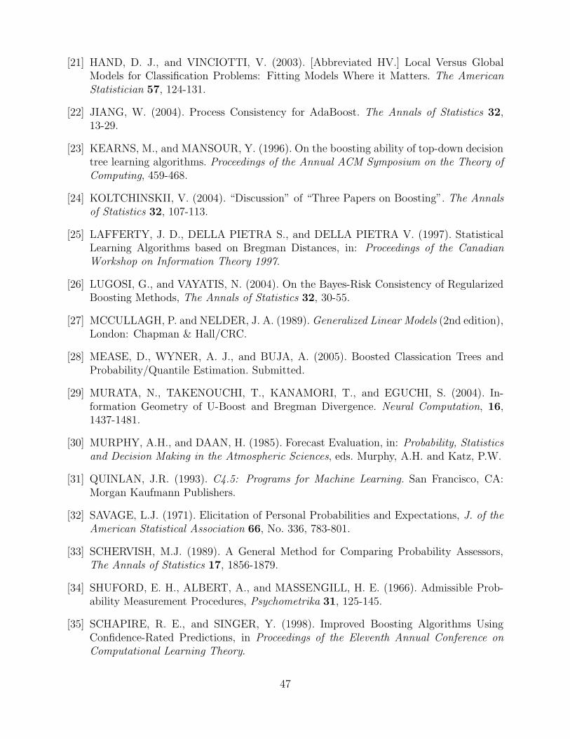
[21] HAND, D. J., and VINCIOTTI, V. (2003). [Abbreviated HV.] Local Versus GlobalModels for Classification Problems: Fitting Models Where it Matters. The AmericanStatistician 57, 124-131.

[22] JIANG, W. (2004). Process Consistency for AdaBoost. The Annals of Statistics 32,13-29.

[23] KEARNS, M., and MANSOUR, Y. (1996). On the boosting ability of top-down decisiontree learning algorithms. Proceedings of the Annual ACM Symposium on the Theory ofComputing, 459-468.

[24] KOLTCHINSKII, V. (2004). “Discussion” of “Three Papers on Boosting”. The Annalsof Statistics 32, 107-113.

[25] LAFFERTY, J. D., DELLA PIETRA S., and DELLA PIETRA V. (1997). StatisticalLearning Algorithms based on Bregman Distances, in: Proceedings of the CanadianWorkshop on Information Theory 1997.

[26] LUGOSI, G., and VAYATIS, N. (2004). On the Bayes-Risk Consistency of RegularizedBoosting Methods, The Annals of Statistics 32, 30-55.

[27] MCCULLAGH, P. and NELDER, J. A. (1989). Generalized Linear Models (2nd edition),London: Chapman & Hall/CRC.

[28] MEASE, D., WYNER, A. J., and BUJA, A. (2005). Boosted Classication Trees andProbability/Quantile Estimation. Submitted.

[29] MURATA, N., TAKENOUCHI, T., KANAMORI, T., and EGUCHI, S. (2004). In-formation Geometry of U-Boost and Bregman Divergence. Neural Computation, 16,1437-1481.

[30] MURPHY, A.H., and DAAN, H. (1985). Forecast Evaluation, in: Probability, Statisticsand Decision Making in the Atmospheric Sciences, eds. Murphy, A.H. and Katz, P.W.

[31] QUINLAN, J.R. (1993). C4.5: Programs for Machine Learning. San Francisco, CA:Morgan Kaufmann Publishers.

[32] SAVAGE, L.J. (1971). Elicitation of Personal Probabilities and Expectations, J. of theAmerican Statistical Association 66, No. 336, 783-801.

[33] SCHERVISH, M.J. (1989). A General Method for Comparing Probability Assessors,The Annals of Statistics 17, 1856-1879.

[34] SHUFORD, E. H., ALBERT, A., and MASSENGILL, H. E. (1966). Admissible Prob-ability Measurement Procedures, Psychometrika 31, 125-145.

[35] SCHAPIRE, R. E., and SINGER, Y. (1998). Improved Boosting Algorithms UsingConfidence-Rated Predictions, in Proceedings of the Eleventh Annual Conference onComputational Learning Theory.

47

[36] SCHAPIRE, R. E. (2002). The Boosting Approach to Machine Learning: An Overview.In: MSRI Workshop on Nonlinear Estimation and Classification.

[37] SHAO, J. (2003). Mathematical Statistics, New York: Springer.

[38] NEWMAN, D. J., HETTICH, S., BLAKE, C. L., and MERZ,C.J. (1998). UCI Repository of machine learning databases[http://www.ics.uci.edu/˜mlearn/MLRepository.html]. Irvine, CA: University ofCalifornia, Department of Information and Computer Science.

[39] WINKLER, R. L (1993). Evaluating Probabilities: Asymmetric Scoring Rules, Man-agement Science 40, No. 11, 1395-1405.

[40] ZHANG, T. (2004). Statistical Behavior and Consistency of Classification Methodsbased on Convex Risk Minimization. The Annals of Statistics (to appear).

48