Embed Size (px)
Citation preview

Some inverse problems arising from elastic scattering by rigid obstacles
This article has been downloaded from IOPscience. Please scroll down to see the full text article.
2013 Inverse Problems 29 015009
(http://iopscience.iop.org/0266-5611/29/1/015009)
Download details:
IP Address: 157.89.65.129
The article was downloaded on 02/03/2013 at 11:18
Please note that terms and conditions apply.
View the table of contents for this issue, or go to the journal homepage for more
Home Search Collections Journals About Contact us My IOPscience

IOP PUBLISHING INVERSE PROBLEMS
Inverse Problems 29 (2013) 015009 (21pp) doi:10.1088/0266-5611/29/1/015009
Some inverse problems arising from elastic scatteringby rigid obstacles
Guanghui Hu1, Andreas Kirsch2 and Mourad Sini3
1 Weierstrass Institute, Mohrenst 39, D-10117 Berlin, Germany2 Department of Mathematics, Karlsruhe Institute of Technology (KIT), D-76131 Karlsruhe,Germany3 RICAM, Austrian Academy of Sciences, Altenbergerst 69, A-4040 Linz, Austria
E-mail: [email protected], [email protected] and [email protected]
Received 16 August 2012, in final form 30 November 2012Published 28 December 2012Online at stacks.iop.org/IP/29/015009
AbstractIn the first part of this paper, it is proved that a C2-regular rigid scatterer in R3
can be uniquely identified by the shear part (i.e. S-part) of the far-field patterncorresponding to all incident shear waves at any fixed frequency. The proof isshort and it is based on a kind of decoupling of the S-part of scattered wavefrom its pressure part (i.e. P-part) on the boundary of the scatterer. Moreover,uniqueness using the S-part of the far-field pattern corresponding to only oneincident plane shear wave holds for a ball or a convex Lipschitz polyhedron.In the second part, we adapt the factorization method to recover the shape ofa rigid body from the scattered S-waves (resp. P-waves) corresponding to allincident plane shear (resp. pressure) waves. Numerical examples illustrate theaccuracy of our reconstruction in R2. In particular, the factorization methodalso leads to some uniqueness results for all frequencies excluding possibly adiscrete set.
(Some figures may appear in colour only in the online journal)
1. Introduction
1.1. Direct elastic scattering problems
Consider a time-harmonic elastic plane wave uin (with the time variation of the form e−iωt ,with a fixed frequency ω > 0) incident on a rigid scatterer D ⊂ R3 embedded in an infiniteisotropic and homogeneous elastic medium in R3. This can be modeled by the reduced Navierequation (or Lame system)
(�∗ + ω2)u = 0, in R3\D, �∗ := μ� + (λ + μ) grad div (1.1)
where u denotes the total displacement field, and λ, μ are the Lame constants satisfying μ > 0,3λ + 2μ > 0. Throughout the paper we suppose that D ⊂ R3 is a bounded open set such that
0266-5611/13/015009+21$33.00 © 2013 IOP Publishing Ltd Printed in the UK & the USA 1

Inverse Problems 29 (2013) 015009 G Hu et al
R3\D is connected, and that the unit normal vector ν to ∂D always points into R3\D. Denotethe linearized strain tensor by
ε(u) := 12
(∇u + ∇u�) ∈ R3×3, (1.2)
where ∇u ∈ R3×3 and ∇u� stand for the derivative of u and its adjoint, respectively. ByHooke’s law the strain tensor is related to the stress tensor via the identity
σ (u) = λ (div u) I + 2με(u) ∈ R3×3, (1.3)
where I denotes the 3 × 3 identity matrix. The surface traction (or the stress operator) on ∂Dis given by
Tνu := σ (u)ν = (2μν · grad + λν div + μν × curl )u. (1.4)
As usual, a · b denotes the scalar product and a × b denotes the vector product of a, b ∈ R3.In this paper the incident wave is allowed to be either a plane shear wave taking the form
uin = uins := q exp(iksx · d), q, d ∈ S2 := {x ∈ R3 : |x| = 1}, (1.5)
with the incident direction d and the polarization direction q satisfying q⊥d, or a plane pressurewave taking the form
uin = uinp := d exp(ikpx · d), d ∈ S2. (1.6)
Here, ks := ω/√
μ and kp := ω/√
λ + 2μ denote the shear wave number and thecompressional wave number, respectively. For a rigid body D, the total field u satisfies the firstkind (Dirichlet) boundary condition
u = 0 on ∂D. (1.7)
Since the scattered field usc := u − uin also satisfies the Navier equation (1.1), it can bedecomposed into the sum
usc := uscp + usc
s , uscp := − 1
k2p
grad div usc, uscs := 1
k2s
curl curl usc,
where the vector functions uscp and usc
s are referred to as the pressure (longitudinal) and shear(transversal) parts of usc respectively, satisfying
(� + k2p)u
scp = 0, curl usc
p = 0, in R3\D,
(� + k2s )u
scs = 0, div usc
s = 0, in R3\D.
Moreover, the scattered field usc is required to satisfy the Kupradze radiation condition (see,e.g. [1])
limr→∞
(∂usc
p
∂r− ikpusc
p
)= 0, lim
r→∞
(∂usc
s
∂r− iksu
scs
)= 0, r = |x|, (1.8)
uniformly in all directions x = x/|x| ∈ S2. The radiation conditions in (1.8) lead to the P-part(longitudinal part) u∞
p and the S-part (transversal part) u∞s of the far-field pattern of usc, given
by the asymptotic behavior
usc(x) = exp(ikp|x|)4π(λ + μ)|x|u∞
p (x) + exp(iks|x|)4πμ|x| u∞
s (x) + O(
1
|x|2)
, |x| → +∞, (1.9)
where u∞p (x) is normal to S2 and u∞
s (x) is tangential to S2. In this paper, we define the far-fieldpattern u∞ of the scattered field usc as the sum of u∞
p and u∞s , that is,
u∞(x) := u∞p (x) + u∞
s (x).
The direct scattering problem (DP) is stated as follows.
2

Inverse Problems 29 (2013) 015009 G Hu et al
(DP: Given a scatterer D ⊂ R3 and an incident plane wave uin, find the total fieldu = uin + usc in R3\D such that the Dirichlet boundary condition (1.7) holds on ∂D andthat the scattered field usc satisfies Kupradze’s radiation condition (1.8).
We refer to the monograph [21] for a comprehensive treatment of the boundaryvalue problems of elasticity, including the boundary conditions of the third and fourthkinds. It is well-known that (see [21]) the direct scattering problem admits one solutionu ∈ C2(R3\D)3 ∩ C1(R3\D)3 if ∂D is C2-smooth, while u ∈ H1
loc(R3\D)3 if ∂D is Lipschitz.
1.2. Inverse elastic scattering problems
We are interested in the following inverse problems arising from elastic scattering.
(IP): Determine the shape of the scatterer D from the knowledge of the transversal far-fieldpattern u∞
s (x) for all x ∈ S2 corresponding to one or more incident plane shear waves ata fixed frequency.(IP
′): Determine ∂D from the longitudinal far-field pattern u∞
p (x) for all x ∈ S2 associatedwith all incident plane pressure waves at a fixed frequency.
There is already a vast literature on inverse elastic scattering problems using the fullfar-field pattern u∞. We refer to the first uniqueness result proved in [12], the sampling typemethods for impenetrable elastic bodies developed in [1, 2] and those for penetrable ones in[4, 25]. Note that in the above works, not only the pressure part of the far-field pattern for allplane shear and pressure waves are needed, but also the shear part of the far-field pattern. Theaim of this paper is to reduce these measurement data to only the S- or P-part of the far-fieldpattern over all directions of measurement corresponding to the same type of plane elasticwaves. We will study uniqueness issues and inversion algorithms for both (IP) and (IP′).
The first uniqueness results using only one type of elastic waves was proved in [11]by D Gintides and M Sini. The authors proved that a C4-smooth obstacle can be uniquelydetermined from the S-part of the far-field pattern corresponding to all incident plane pressure(or shear) waves. Moreover, the same uniqueness result remains valid using the shear partof the far-field pattern. This shows that any of the two different types of waves is enough todetect obstacles at a fixed frequency. The arguments in [11], which are applicable for boththe two and three dimensions and also for different boundary or transmission conditions,mainly rely on the asymptotic analysis, near the boundary of the obstacle, of the pressure andshear parts of reflected solutions when the P-part or S-part of the fundamental solution to theNavier equation (1.1) is taken as an incident field. This analysis requires the C4-smoothnessassumption mentioned above. We also refer to [10] for a MUSIC type algorithm applied tothe detection of point-like scatterers using only one type of scattered elastic waves. However,apart from the inversion scheme proposed in [11], no inversion algorithms have been proposedand tested for identifying an extended obstacle using one type of elastic waves.
In the first half of this paper, we present a new uniqueness proof to (IP) for C2-smoothobstacles, following Isakov’s idea of using singular solutions (see [15]). Since only the S-part of scattered fields can be reconstructed from the transversal far-field pattern, a boundarycondition (see (2.16) or (2.31)) will be derived in order to couple the incident shear waveand the S-part of scattered waves on ∂D. This shows some kind of decoupling of the S-partof the scattered waves from the P-parts. Based on this observation, our proof seems morestraightforward than the arguments used in [11] and can be extended to Lipschitz scatterersas well as the fourth kind boundary conditions. Moreover, we prove that a ball or a convexpolyhedron can be uniquely identified from the S-part of the far-field pattern correspondingto only one incident shear wave. However, our approach (essentially the boundary condition
3

Inverse Problems 29 (2013) 015009 G Hu et al
(2.31)) is only valid for problem (IP) in 3D and cannot be generalized to problem (IP′); seeremarks 2.4 and 2.5 for a brief discussion of what goes wrong in these cases.
In the second half, we adapt the factorization method to recover ∂D from the scatteredS-waves (resp. P-waves) for all incident plane shear (resp. pressure) waves. In particular, thefactorization method also implies some uniqueness results provided ω2 is not the Dirichleteigenvalue of −�∗ in D. It is well known that such eigenvalues form a discrete set withthe only accumulating point at infinity. Our numerical experiments demonstrate satisfactoryresults from the S-part or P-part of the far-field pattern compared to the reconstruction fromthe full far-field pattern.
2. Uniqueness using the S-part of the far-field pattern
Concerning the regularity of the boundary ∂D, it is supposed that either ∂D is of class C2 orD is a convex polyhedron defined as below.
Definition 2.1. A scatterer D ⊂ R3 is called a convex polyhedron if D is the intersection of afinite number of half spaces with connected, non-void and bounded interior.
Note that the boundary of a convex polyhedron consists of a finite number of cellswithout any cracks. Here a cell is defined as the closure of an open connected subset of atwo-dimensional plane. As a notation convention we shall employ the symbol
U (·) = U (·; d, q, D), U = usc, u, u∞p , u∞
s , uscp , usc
s ,
to indicate the dependence of U (·) on the obstacle D, the incident direction d and thepolarization q. In some cases we write U (·; d, q, D) = U (·; d, q) for brevity. Here is ourmain result on the uniqueness of (IP).
Theorem 2.2. If there are two scatterers D and D such that
u∞s (x; d, q) = u∞
s (x; d, q), for all x, d, q ∈ S2, q⊥d, (2.1)
then D = D. Moreover, if D and D are both balls or convex polyhedral scatterers, then therelation
u∞s (x; d0, q0) = u∞
s (x; d0, q0), for all x ∈ S2, (2.2)
with one incident direction d0 ∈ S2 and one polarization q0 ∈ S2 such that q0⊥d0 is enoughto imply that D = D.
Theorem 2.2 will be proved in section 2.1 for general C2-smooth scatterers, in section 2.2for balls and in section 2.3 for convex polyhedral scatterers. To prove theorem 2.2, we needthe fundamental solution (Green’s tensor) to the Navier equation given by
(x, y) = k2s
4πω2
eiks|x−y|
|x − y| I + 1
4πω2gradx grad�
x
[eiks|x−y|
|x − y| − eikp|x−y|
|x − y|]
. (2.3)
Let the vector a ∈ S2 be fixed. Denote by Gin(x; y) = Gin(x; y, a) the shear part of (x, y)a,i.e. for x = y,
Gin(x; y, a) := 1
k2s
curlx curlx [(x, y)a]
= k2s
4πω2
[eiks|x−y|
|x − y| I + 1
k2s
gradx grad�x
eiks|x−y|
|x − y|]
a. (2.4)
In the sequel, we view Gin(x; y, a) as an incident point source wave, and correspondingly,denote by Gsc(x; y, a), G(x; y, a), G∞
s (x; y, a) the scattered, total waves and the transversal
4

Inverse Problems 29 (2013) 015009 G Hu et al
far-field pattern associated with Gin, respectively. Since the function Gin(x; y, a) satisfies (seee.g. [23])
curl xcurl x Gin(x; y, a) − k2s Gin(x; y, a) = k2
s
4πω2δ(x − y)a,
for x = y, it is easy to check that
(�∗ + ω2)Gin = −δ(x − y)a, (2.5)
i.e. Gin(x; y, a) is one of Green’s functions to the Navier equation (1.1). The relation (2.5) willbe used in section 2.1 below.
2.1. Uniqueness for a general scatterer
The aim of this section is to prove the first assertion of theorem 2.2, i.e. the unique determinationof a C2-smooth scatterer using only the S-part of the far-field pattern for all incident shearwaves. Our proof is based on the mixed reciprocity relation between the transversal far-fieldpattern G∞
s (x; y, a) corresponding to Gin and the S-part uscs (x; d, q) of the scattered field
corresponding to uins . The following lemma 2.3 extends the mixed reciprocity relations of R.
Potthast in acoustic and electromagnetic scattering (see [24]) to the elastic case.
Lemma 2.3. For y ∈ R3\D, we have
q · G∞(−d; y, a) = q · G∞s (−d; y, a) = a · usc
s (y; d, q) for all q⊥d. (2.6)
Proof. Since Gsc and usc both fulfil the Kupradze radiation condition, there holds∫∂D
Gsc(z) · Tν(z)usc(z) − Tν(z)G
sc(z) · usc(z) ds(z) = 0, (2.7)
where Tν is the stress operator defined in (1.4). Note that in (2.7) we wrote Gsc(z; y, a) = Gsc(z)and usc(z; d, q) = usc(z) for simplicity. This notational rule also applies to the total fieldsG(z), u(z) and the transversal far-field patterns G∞
s (x), u∞s (x). From Betti’s integral theorem,
for radiating solutions Gsc ∈ C2(R3\D)3 ∩ C1(R3\D)3 to the Navier equation, one can derivethe integral representation
Gsc(x) =∫
∂D[Tν(z)(x, z)]�Gsc(z) − (x, z)Tν(z)G
sc(z) ds(z), x ∈ R3\D, (2.8)
where Tν = (Tν1, Tν2, Tν3) with j being the jth column of . Letting |x| → ∞ in(2.8) and using the definitions of u∞
p and u∞s in (1.9), it follows that (see also [1])
G∞p (x) =
∫∂D
{[Tν(z) {xx�e−ikpx·z}]�Gsc(z) − xx�e−ikpx·z Tν(z)Gsc(z)} ds(z), (2.9)
and
G∞s (x) =
∫∂D
{[Tν(z){(I − xx�) e−iksx·z}]�Gsc(z) − (I − xx�) e−iksx·zTν(z)Gsc(z)} ds(z). (2.10)
Since q · d = 0, we deduce from (2.9), (2.10) with x = −d that
q · G∞p (−d) = 0, (2.11)
q · G∞s (−d) =
∫∂D
{Gsc(z) · Tν(z) [qeiksd·z] − qeiksd·z · Tν(z)G
sc(z)}
ds(z). (2.12)
5

Inverse Problems 29 (2013) 015009 G Hu et al
Combining (2.11), (2.12) and (2.7) gives
q · G∞(−d; y, a)
= q · G∞s (−d; y, a)
=∫
∂D{Gsc(z) · Tν(z) u(z; d, q) − u(z; d, q) · Tν(z)G
sc(z)} ds(z). (2.13)
This proves the first identity in lemma 2.3. Again using Betti’s integral theorem, we have (cf(2.8))
usc(x) =∫
∂D{[Tν(z)(x, z)]�usc(z) − (x, z)Tν(z)u
sc(z)} ds(z), x ∈ R3\D,
implying that
a · uscs (x; d, q)
= a · 1
k2s
curl xcurl x{usc(x; d, q)
}= a · 1
k2s
curl xcurl x
{∫∂D
[Tν(z)(x, z)]�usc(z) − (x, z)Tν(z)usc(z) ds(z)
}=
∫∂D
{usc(z) · Tν(z)Gin(x; z) − Tν(z)u
sc(z) · Gin(x; z)} ds(z).
Moreover, applying Betti’s second integral theorem to uin and Gin in D yields
0 =∫
∂D{uin(z) · Tν(z)G
in(x; z) − Tν(z)uin(z) · Gin(x; z)} ds(z), x ∈ R3\D.
Adding up the previous two equalities with x = y, we arrive at
a · uscs (y; d, q) =
∫∂D
{u(z) · Tν(z)Gin(y; z) − Tν(z)u(z) · Gin(y; z)} ds(z)
=∫
∂D{u(z) · Tν(z)G
in(z; y) − Tν(z)u(z) · Gin(z; y)} ds(z), (2.14)
where the last equality sign follows from the symmetry of Gin(z; y) in z and y. Combining(2.14) and (2.13), we find
q · G∞s (−d; y, a) − a · usc
s (x; d, q)
=∫
∂D{[Tν(z) u(z; d, q)]� · G(z) − u(z; d, q) · Tν(z)G(z)} ds(z)
= 0.
This proves the second identity in (2.6). �
Our proof of the first assertion of theorem 2.2 relies on a refinement of the arguments in[15, 18, 12] using singular solutions and the simplified version (see e.g. [23, theorem 14.6])using the mixed reciprocity relations. Note that in our proof only the S-part of scattered fieldscan be uniquely determined from the transversal far-field pattern.
Proof of theorem 2.2 for a general obstacle. Let D and D be the two rigid obstacles intheorem 2.2 satisfying (2.1). Let � denote the unbounded connected component of R3\D ∪ D,and define the incident point source waves Gin(x; y, a) as in (2.4) for y ∈ �, with somepolarization vector a ∈ S2 to be determined later. From the identity (2.1) and the Rellichlemma it follows that
a · uscs (y; d, q) = a · usc
s (y; d, q), for all d, q ∈ S2, d⊥q, y ∈ �,
6

Inverse Problems 29 (2013) 015009 G Hu et al
which, combined with the reciprocity relation in lemma 2.3, gives
q · G∞s (−d; y, a) = q · G∞
s (−d; y, a), for all d, q ∈ S2, d⊥q, y ∈ �.
Together with the relation d · G∞s (−d; y, a) = d · G∞
s (−d; y, a) = 0, the previous identityimplies
G∞s (x; y, a) = G∞
s (x; y, a), for all x ∈ S2, y ∈ �.
Again applying the Rellich lemma, we have the coincidence of the shear parts of Gsc and Gsc,
Gscs (z; y, a) = Gsc
s (z; y, a), for all z, y ∈ �. (2.15)
Since the compressional part Gscp of Gsc is irrotational and the total field G(z; y) =
Gin(z; y) + Gscp (z; y) + Gsc
s (z; y) = 0 on ∂D for all y ∈ R3\D, we get
ν(z) · curl z(Gin(z; y) + Gsc
s (z; y)) = ν(z) · curl zG(z; y)
= − Divz(ν(z) × G(z; y))
= 0 (2.16)
for z ∈ ∂D, where Div(·) stands for the surface divergence operator which is well-defined onthe C2-smooth boundary ∂D. Analogously, there holds ν(z) · curl z(Gin(z; y) + Gsc
s (z; y)) = 0for z ∈ ∂D.
Assuming that D = D, we next derive a contradiction from (2.15) and the boundarycondition (2.16). Without loss of generality, we may choose a point y∗ ∈ ∂� and a vectora∗ = a∗(y∗) ∈ S2 such that y∗ ∈ ∂D, y∗ /∈ ∂D and a∗×ν(y∗) = 0. In particular, for sufficientlylarge N ∈ N+, we may assume yn = y∗ + a∗(y∗)/n ∈ �, n � N. Choose the polarizationvector a ∈ S2 such that a · (ν(y∗) × a∗) = 0. Taking z = y∗, y = yn in (2.15) and settingν = ν(y∗) , we find
ν(y∗) · curl z(Gscs (z; yn))|z=y∗ = ν(y∗) · curl z(G
scs (z; yn))|z=y∗ , for all n � N. (2.17)
On the one hand, the right hand side of (2.17) is uniformly bounded, due to the well-posednessof the forward scattering problem and the fact that y∗ ∈ R3\D. On the other hand, it followsfrom (2.16) and the definition of Gin(z, y) that
ν(y∗) · curl z(Gscs (z; yn))|z=y∗ = − ν(y∗) · curl z(G
in(z; yn))|z=y∗
= k2s
4πω2ν(y∗) ·
(a × ∇z
eiks|z−yn|
|z − yn|)∣∣∣∣
z=y∗
= k2s
4πω2(ν(y∗) × a) ·
[∇z
eiks|z−yn|
|z − yn|]∣∣∣∣
z=y∗
= k2s
4πω2(iksn − n2) exp(iks/n)(ν(y∗) × a) · a∗
which tends to infinity as n → ∞, since (ν(y∗) × a) · a∗ = 0. This contradiction implies thatD = D. �
Remark 2.4. Our arguments do not work using the longitudinal far-field pattern of plane shearwaves. To see this, we need the compressional part of (x, y)a given by
H in(x; y, a) = − 1
k2p
gradx divx[(x, y)a] = − 1
4πω2gradx grad�
x
eikp|x−y|
|x − y| a, x = y.
Similarly, denote by H∞s (x; y, a), H∞
p (x; y, a) the transversal and longitudinal far-field patternassociated with the incident wave H in. Analogously to lemma 2.3, one can prove the reciprocityrelation
q · H∞(−d; y, a) = q · H∞s (−d; y, a) = a · usc
p (y; d, q), y ∈ R3\D, (2.18)
7

Inverse Problems 29 (2013) 015009 G Hu et al
for all d⊥q. However, since curl xH in(x; z) = 0 for x = z we cannot generalize the argumentsfrom section 2.1 to the present case by employing the boundary condition (2.16) with Gsc
sreplaced by Hsc
s . Further, we point out that our proof cannot be applied to the second (Neumann)or third kind boundary conditions, even in the case of two-dimensional elastic scattering.
Remark 2.5. Our approach for proving the first assertion of theorem 2.2 cannot apply toincident plane pressure waves. Given the incident pressure wave uin
p defined in (1.6), we canestablish the following mixed reciprocity relations
d · G∞(−d; y, a) = d · G∞p (−d; y, a) = a · usc
s (y; d), (2.19)
d · H∞(−d; y, a) = d · H∞p (−d; y, a) = a · usc
p (y; d), (2.20)
for all d⊥q, where uscs and usc
p denote the S-part and P-part of the scattered field usc(y; d)
corresponding to uinp . Again the boundary condition (2.16) cannot be employed with the
transversal part Gscs replaced by the irrotational longitudinal part Gsc
p or Hscp .
Note that the mixed reciprocity relations (2.6), (2.18), (2.19) and (2.20) remain true forother boundary conditions and penetrable scatterers. It is worth mentioning the more generalidentity established in [3, theorem 7] between full far-field patterns, the proof of which isbased on the reciprocity relation for two point source incidences. Our lemma 2.3 providesa more straightforward proof of these mixed reciprocity relations. See also [3, 7, 8] for thereciprocity principles due to two incident plane elastic waves.
2.2. Uniqueness for balls
Continuation of the proof of theorem 2.2. To prove the second assertion of theorem 2.2for balls, we will follow Kress’ arguments from [19] for proving uniqueness in inverseelectromagnetic scattering by perfectly conducting balls. Let Q be a rotation matrix in R3. Wehave the following relation between u∞(x; d, q, D) and u∞(x; d, q, QD) (see [22, section 5])
Qu∞α (x; d, q, D) = u∞
α (Qx; Qd, Qq, QD), for all x, d, q ∈ S2, q⊥d, α = p or s. (2.21)
If D is a ball centered at the origin, then the relation (2.21) with α = s reduces to
Qu∞s (x; d, q, D) = u∞
s (Qx; Qd, Qq, D), for all x, d, q ∈ S2, d⊥q. (2.22)
Letting D and D be the two balls given in theorem 2.2, one can conclude from the explicitexpression of the S-part of the scattered field that usc
s (x; d, q) resp. uscs (x; d, q) can be
analytically extended into the interior of D resp. D with the exception of its center; seeappendix for the proof in elasticity. Since usc
s (x; d, q) and uscs (x; d, q) are radiating solutions to
the Helmholtz equation, by the Rellich lemma the centers of D and D must coincide. Withoutloss of generality we may assume the center is located at the origin. Thus QD = D andQD = D for any rotation matrix Q. We claim that the identity (2.2) with one incident directiond0 and one polarization direction q0 implies the relation (2.1) for all incident and polarizationdirections. Therefore, the uniqueness for balls with one incident wave follows directly fromthe first assertion in theorem 2.2. In fact, given d1, q1 ∈ S2 such that d1⊥q1, there exists arotation Q satisfying either Qq0 = q1, Qd0 = d1 or Qq0 = −q1, Qd0 = d1. Applying therotation Q to both sides of (2.2) and making use of (2.22) for D and D, we obtain
u∞s (Qx; Qd0, Qq0, D) = u∞
s (Qx; Qd0, Qq0, D), for all x ∈ S2,
which implies
u∞s (Qx; d1, q1, D) = u∞
s (Qx; d1, q1, D), for all x ∈ S2. (2.23)
8

Inverse Problems 29 (2013) 015009 G Hu et al
Note that u∞s and u∞
s depend linearly on the polarization. By the arbitrariness of x, d1, q1 ∈ S2,we arrive at the identity (2.1). Therefore, we obtain D = D as a consequence of the uniquenessresult in theorem 2.2 for all incident and polarization directions. This completes the proof oftheorem 2.2 for balls. �
The well-known Karp’s theorem in two-dimensional acoustics states that, a scatterer is adisc if the far-field pattern only depends on the angle between the incident and observationdirections; see e.g. [6, chapter 5.1] in acoustics and [6, chapter 7.1] in electromagnetics. Theelastodynamic analogue of Karp’s theorem was proved in [22] by applying the uniquenessresults in inverse elastic scattering with an infinite number of incident waves. Following [22],we next prove another elastodynamic analogue of Karp’s theorem using only the transversalfar-field pattern.
Corollary 2.6. Suppose that u∞s (x; d0, p0, D) is the S-part of the far-field pattern associated
with the incident shear wave (1.5) with d = d0, q = q0. Then, D is a ball if there holds for anyrotational matrix Q that
Qu∞s (x; d0, q0, D) = u∞
s (Qx; Qd0, Qq0, D), for all x ∈ S2. (2.24)
Proof. It follows from (2.22) and (2.24) that
u∞s (Qx; Qd0, Qq0, QD) = u∞
s (Qx; Qd0, Qq0, D), for all x ∈ S2. (2.25)
With the similar arguments used to derive (2.23), we deduce from (2.25) that
u∞s (x; d, q, QD) = u∞
s (x; d, q, D), for all x, q, d ∈ S2, q⊥d. (2.26)
Applying theorem 2.2, we conclude that QD = D for all rotational matrices Q. Hence D is aball. �
Remark 2.7. The results in section 2.2 are also true for other boundary conditions usingP- or S-part of the scattered waves corresponding to P- or S-incident waves, since the argumentsare based on the corresponding results using many incident waves.
2.3. Uniqueness for convex polyhedrons
Continuation of the proof of theorem 2.2. Suppose that (2.2) holds for two different convexLipschitz polyhedral obstacles D and D. Without loss of generality, we may always assumethat there exists a corner point A ∈ R3 of ∂D such that A /∈ ∂D. Denote by � j, j = 1, 2, 3
three cells of ∂D meeting at A, and by � j the extension of � j to R3\D. Obviously, each cell
� j can be extended to infinity in R3\D due to the convexity of both D and D. Since the totalfield u = uin
s + uscs + usc
p = 0 on ∂D, there holds the boundary condition
ν j · curl u = −Div (ν j × u) = 0 on � j, j = 1, 2, 3, (2.27)
with ν j being the normal direction of � j. Note that the differential operators in (2.27) makesense, because � j is flat so that u is smooth up to the boundary except for a finite number ofcorner points and edges. Analogously to (2.16), we have
ν j · curl(uin
s + uscs
) = 0 on � j, j = 1, 2, 3, (2.28)
9

Inverse Problems 29 (2013) 015009 G Hu et al
since curl uscp = 0 in R3\D. By the Rellich lemma, the relation (1.9) yields usc
s (x) = uscs (x) for
all x ∈ � := R3\(D ∪ D). In particular, we have curl uscs = curl usc
s on � j\D using standardelliptic regularity of usc
s (x) and uscs (x). Thus, the identity (2.28) implies the relation
ν j · curl(uin
s + uscs
) = 0 on � j\D, j = 1, 2, 3, (2.29)
which combined with the analyticity of the function U := uin + uscs in R3\D gives
ν j · curl(uin
s + uscs
) = 0 on � j, j = 1, 2, 3,
that is,
iksν j · (d0 × q0) exp(iksx · d0) + ν j · curl uscs (x) = 0 on � j, j = 1, 2, 3. (2.30)
Letting |x| → +∞ in (2.30) for x ∈ � j, we obtain ν j · (d0 × q0) = 0, j = 1, 2, 3, sincecurl usc
s (x) decays uniformly in all directions (see the radiation condition in (1.8)). Noting thatν j are three linearly independent vectors, we get d0 × q0 = 0. However, this is impossiblebecause d0⊥q0. This contradiction gives D = D. �
Remark 2.8. We have no uniqueness for non-convex polyhedrons. If D and D are notnecessarily convex polyhedrons, one can only conclude that the convex hulls of D and Dcoincide. For global uniqueness results within non-convex polyhedral obstacles, we refer to[9] by J Elschner and M Yamamoto using the full far-field pattern of one or several incidentplane elastic waves. Their proofs were based on the reflection principle for the Navier equationunder the third or fourth kind boundary conditions. However, there seems no reflection principlefor the Navier equation under the Dirichlet boundary condition.
To sum up, our uniqueness proofs for (IP) are essentially based on the identity
ν · curl (uins + usc
s ) = −Div(ν × u) = 0 on ∂D. (2.31)
One may observe further that the relation (2.31) is still true under the fourth kind boundaryconditions (see e.g. [21])
ν × u = 0, ν · Tu = 0 on ∂D, (2.32)
where T is the stress operator given in (1.4). Hence, we have
Corollary 2.9. The uniqueness results in theorem 2.2 remain valid if the Dirichlet boundarycondition (1.7) is replaced by the fourth kind boundary conditions (2.32).
Relying on the boundary condition (2.31), some existing numerical methods, e.g., linearsampling method [6], probe method [14] or singular sources method [24] can be utilized torecover the shape of a rigid scatterer from only the transversal far-field pattern associated withall incident shear waves. We next adapt the factorization method established in [16] (see alsothe monograph [17]) to this case. Moreover, the factorization method also allows us to handlethe problem (IP′) using only pressure waves.
3. Factorization method
We first review the F∗F-method in inverse elastic scattering problems (see [1]) involving thefull far-field pattern, and then use a modified version to reconstruct ∂D using only one part ofthe far-field pattern. In this section, the boundary ∂D of D ⊂ R3 is allowed to be Lipschitz,and D may consist of several components.
For g(d) ∈ L2(S2)3, d ∈ S2, there holds the decomposition
g(d) = gs(d) + gp(d), gs(d) := d × g(d) × d, gp(d) := (g(d) · d) d, (3.1)
10
Inverse Problems 29 (2013) 015009 G Hu et al
where gs(d) belongs to the space
L2s (S
2) := {gs : S2 → C3 : gs(d) · d = 0, |gs| ∈ L2(S2)} (3.2)
of transversal vector fields on S2, while gp(d) belongs to the space
L2p(S
2) := {gp : S2 → C3 : gp(d) × d = 0, |gp| ∈ L2(S2)}of longitudinal vector fields on S2. For g ∈ L2(S2)3, introduce the incident field
ving (x) :=
∫S2
[gs(d) eiksx·d + gp(d) eikpx·d] ds(d).
The far-field pattern v∞g corresponding to the incident wave vin
g defines the far-field operatorF from L2(S2)3 into itself by Fg = v∞
g . Denote by v∞g,s ∈ L2
s (S2) and v∞
g,p ∈ L2p(S
2) the S-partand P-part of v∞
g , which are defined in the same way as in (3.1). The following properties ofF have been derived in [1].
Lemma 3.1.
(i) The far-field operator F is compact, normal with dense range in L2(S2)3, and the scatteringmatrix I + i
2πF is unitary. Here I denotes the identity operator.
(ii) If ω2 is not the Dirichlet eigenvalue of the operator −�∗ in D, then F is injective and itsnormalized eigenfunctions form a complete orthonormal system in L2(S2)3.
Let the Herglotz operator H : L2(S2)3 → H1/2(∂D)3 be defined by Hg := ving (x)|∂D.
Then, the adjoint operator H∗ : H−1/2(∂D)3 → L2(S2)3 of H is given by
H∗ϕ(x) :=∫
∂D[ϕs(y) e−iksy·x + ϕp(y) e−ikpy·x ds(y)], x ∈ S2,
which is, by our normalization, just the far-field pattern of the function
w(x) =∫
∂D(x, y)ϕ(y) ds(y), x /∈ D,
where (x, y) is Green’s tensor to the Navier equation (see (2.3)). Note that, for some non-trivial vector a ∈ S2, the far-field pattern of the function x → (x, y)a is given by
∞y (x) = e−iksx·y[x × (a × x)] + e−ikpx·y(x · a)x, for all y ∈ R3. (3.3)
Define the data-to-pattern operator G : H1/2(∂D)3 → L2(S2)3 by f → v∞, where v∞ is thefar-field pattern of the radiating solution v which satisfies the Navier equation (1.1) in R3\Dwith the boundary data f ∈ H1/2(∂D)3. With these definitions, we have the decomposition
Fg = −GHg, H∗(ϕ) = G(w|∂D) = GS(ϕ), (3.4)
where S : H−1/2(∂D)3 → H1/2(∂D)3 denotes the classical single-layer operator
(Sϕ)(x) =∫
∂D(x, y)ϕ(y) ds(y), x ∈ ∂D.
From (3.4), it follows the factorization
F = −GS∗G∗. (3.5)
The sampling method developed in [1] is based on the factorization (3.5) combined with someproperties of the single-layer operator S (see [1, lemmas 6.1, 6.2]), which extends Kirsch’sresults [16] from acoustic scattering to the elastic case in 3D. It is seen from [1, section 6] thatall the assumptions of [17, theorem 1.23] are fulfilled, so that we have (see [1, theorem 6.3])
Lemma 3.2. If ω2 is not the Dirichlet eigenvalue of −�∗ in D, then the ranges of G and(F∗F )1/4 coincide.
11

Inverse Problems 29 (2013) 015009 G Hu et al
Further, it is proved in [1, theorem 6.4] that the function ∞y (x) given in (3.3) belongs
to the range of G if and only if y ∈ D. Thus, by lemma 3.2 we can characterize the scattererD in terms of the range of (F∗F )1/4. Using the orthogonal system of eigenfunctions of F , itfollows from Picard’s theorem that
Theorem 3.3. If ω2 is not the Dirichlet eigenvalue of −�∗ in D, then
y ∈ D ⇐⇒ W (y) :=[ ∞∑
n=1
|(gn,∞y )L2(S2 )|2|ηn|
]−1
> 0, (3.6)
where ηn ∈ C denote the eigenvalues of F with the corresponding orthonormal eigenfunctionsgn ∈ L2(S2)3, and (·, ·)L2(S2 ) denotes the usual inner product in the space L2(S2)3.
Remark 3.4. Analogously to the factorization method in acoustics, the eigensystem (ηn, gn)
in theorem 3.3 can be replaced by the eigensystem of F# defined by
F# := |Re F| + |Im F|, Re F := 12 [F + F∗], Im F := 1
2i [F − F∗].
This is mainly due to the inequality1√2[|Re ηn| + |Im ηn|] � |ηn| � |Re ηn| + |Im ηn|.
We note that the eigensystem of F used in theorem 3.3 are determined by both the P-partand S-part of the far-field pattern for all incident pressure and shear plane waves. Relying onthe previous analysis, we now turn to the study of the factorization method for (IP) and (IP′)where the incident fields consist of plane shear or pressure waves only.
Introduce the orthogonal projection operator Ps : L2(S2)3 → L2s (S
2)3, where L2s (S
2)3
is given in (3.2), i.e. Ps g(d) = gs(d). The adjoint P∗s : L2
s (S2)3 → L2(S2)3 of Ps is just
the inclusion from L2s (S
2)3 to L2(S2)3. Therefore, the operator Fs := Ps F P∗s , which maps
L2s (S
2)3 to L2s (S
2)3, is the projection of the restriction of F to L2s (S
2)3. By (3.5), it has thefactorization
Fs := PsFP∗s = −(PsG)S∗(PsG)∗. (3.7)
In contrast to F the operator Fs fails to be normal. Therefore, theorem 1.23 of [17] is notapplicable. We further note that the characterization (3.6) is essentially based on the normalityof the far-field operator F and the unitarity of the scattering operator I + i
2πF . Instead of [17,
theorem 1.23], we now apply the range identity [17, theorem 2.15] to the operator Fs.
Lemma 3.5. If ω2 is not the Dirichlet eigenvalue of −�∗ in D, then the ranges of PsG andF1/2
s# coincide, where Fs# := |Re Fs| + |Im Fs|.
Proof. We need to justify all the conditions in [17, theorem 2.15]. Obviously, the operatorPsG : H1/2(∂D)3 → L2
s (S2)3 is compact with dense range, since the data-to-pattern operator
G : H1/2(∂D)3 → L2(S2)3 is compact with dense range. We collect the following propertiesof the single-layer operator S from [1, section 6].
(a) ImS = 12i (S − S∗) is non-negative, that is,
Im(Sϕ, ϕ)L2(∂D) � 0 for all ϕ ∈ Cα(∂D)3.
More generally, it holds that
Im〈ϕ, Sϕ〉 � 0 for all ϕ ∈ H−1/2(∂D)3,
where 〈·, ·〉 denotes the duality pairing in⟨H−1/2(∂D)3, H1/2(∂D)3
⟩.
12

Inverse Problems 29 (2013) 015009 G Hu et al
(b) The strict inequality in the assertion (a) holds for all ϕ = 0 provided ω2 is not an interiorDirichlet eigenvalue.
(c) Let Si be the single-layer operator corresponding to ω = i. Then Si is self-adjoint andcoercive; that is, there exists c > 0 such that
〈ϕ, Siϕ〉 � c‖ϕ‖2H−1/2(∂D)
for all ϕ ∈ H−1/2(∂D)3.
Furthermore, S − Si is compact from H−1/2(∂D)3 into H1/2(∂D)3.
Now, the range identity of theorem 2.15 of [17] yields that the ranges of PsG and F1/2s#
coincide. �To characterize the scatterer D in terms of the operator Fs, we need the following lemma.
Lemma 3.6. Let the function ∞y (x) be given as in (3.3). The function Ps(
∞y ) belongs to the
range of Ps G if and only if y ∈ D.
Proof. If y ∈ D, then the trace of the function x → (x, y)a on ∂D belongs to H1/2(∂D)3.Thus Ps(
∞y ) = PsG( f ) with f = (x, y)a|x∈∂D. Assume that Ps(
∞y ) = PsG( f ) for some
f ∈ H1/2(∂D)3, that is, the S-part ∞y,s of ∞
y coincides with the S-part v∞s of v∞, where v∞
is the far field pattern of the radiating solution v in H1loc(R
3\D)3 with v = f on ∂D. Denoteby [(x, y)a]s and vs the shear parts of (x, y)a and v, respectively. If y /∈ D, it followsfrom the Rellich identity and the unique continuity of solutions of the Helmholtz equation thatvs(x) = [(x, y)a]s for all x ∈ R3\{D ∪ {y}}. Therefore,
curl x[(x, y)a]s = curl vs = curl v ∈ L2loc(R
3\D)3. (3.8)
However, it follows from (2.4) that
curl x[(x, y)a]s = curl xGin(x; y, a) ∼ O(|x − y|−2), as x → y in R3\{D ∪ {y}},which contradicts (3.8). Thus y ∈ D. �
Combining the previous two lemmas, we get
Theorem 3.7. If ω2 is not the Dirichlet eigenvalue of −�∗ in D, then
y ∈ D ⇐⇒ Ws(y) :=[ ∞∑
n=1
|(gn,∞y,s)L2(S2)|2ηn
]−1
> 0, (3.9)
where ∞y,s := Ps(
∞y ) = exp(−iksx · y) [x × (a × x)] for some a ∈ S2, and {ηn, gn} is an
eigensystem of the positive operator Fs# defined in lemma 3.5.
The same technique is also applicable to the inverse problem (IP’). Let Pp denote theorthogonal projection operator from L2(S2)3 to L2
p(S2)3, i.e. Ppg(d) = gp(d). Define the
operator Fp := Pp F P∗p . We then have the factorization
Fp = −(PpG)S∗(PpG)∗. (3.10)
The arguments in lemmas 3.5 and 3.6 can be immediately applied to the operator Pp. As aconsequence, we obtain
Theorem 3.8. If ω2 is not the Dirichlet eigenvalue of −�∗ in D, then
y ∈ D ⇐⇒ Wp(y) :=[ ∞∑
n=1
|(gn,∞y,p)L2(S2 )|2ηn
]−1
> 0, (3.11)
where ∞y,p := Pp(
∞y ) = exp(−ikpx·y)(x·a)x for some a ∈ S2, and {ηn, gn} is an eigensystem
of the (positive) operator Fp# := |Re Fp| + |Im Fp|.13

Inverse Problems 29 (2013) 015009 G Hu et al
Obviously, theorems 3.7 and 3.8 provide new uniqueness results by using only one typeof elastic waves.
Corollary 3.9. Assume that the rigid body D ∈ R3 has a Lipschitz boundary, and that ω2 is notthe Dirichlet eigenvalue of −�∗ in D. Then D can be uniquely identified from the S-part of thefar-field pattern for all incident plane shear waves. The uniqueness is also true by employingthe P-part of the far-field pattern for all incident plane pressure waves.
4. Numerical examples
We suppose that D = �×R ⊂ R3 is an infinitely long cylinder, and turn to the presentation ofsome numerical simulations in R2 for constructing the boundary ∂� ⊂ R2. We refer to [2] forthe linear sampling method and F∗F-method in the two-dimensional inverse elastic scatteringwhere the full far-field pattern is involved.
Recall that in R2, Green’s tensor of the Navier equation is given by
�(x, y) := 1
4μH (1)
0 (ks|x − y|)I + i
4ω2gradx grad�
x
[H (1)
0 (ks|x − y|) − H (1)
0 (kp|x − y|)]for x, y ∈ R2, x = y, where H (1)
0 (t) denotes the Hankel function of the first kind and of orderzero. To be consistent with the presentation in R3 we define the far-field pattern
u∞ := xu∞p (x) + x⊥u∞
s (x), (x1, x2)⊥ := (−x2, x1).
Here, note that u∞p (x) = u∞(x) · x, u∞
s (x) = u∞(x) · x⊥ are two scalar functions given by theasymptotic behavior
usc(x) = exp(ikpx + iπ/4)√8πkp|x|
u∞p (x)x + exp(iksx + iπ/4)√
8πks|x|u∞
s (x)x⊥ + O(|x|−3/2), |x| → ∞.
With this normalization, for a fixed vector a ∈ C2 the far-field pattern �∞y (x) of the function
x → �(x, y)a is given by
�∞y (x) = exp(−ikpx · y)(x · a)x + exp(−iksx · y)(x⊥ · a)x⊥ =: �∞
y,p(x)x + �∞y,s(x)x⊥.
We make the ansatz for the scattered field usc in the form
usc(x) =∫
∂�
�(x, y)φ(y) ds(y), x ∈ R3\�,
with some function φ(y) ∈ L2(∂�)2. Assume that ∂� can be parameterized by(r1(t), r2(t)), t ∈ [0, 2π ]. Then the P-part and S-part of the far-field pattern of usc are givenby
u∞p (x) =
∫ 2π
0e−ikpx·(r1(t),r2(t))�[x · φ(r1(t), r2(t))]
√r′
1(t)2 + r′
2(t)2 dt,
u∞s (x) =
∫ 2π
0e−iksx⊥·(r1(t),r2(t))�[x⊥ · φ(r1(t), r2(t))]
√r′
1(t)2 + r′
2(t)2 dt,
respectively, in terms of the density function φ.Now, let N plane pressure waves dj exp(ikpx·d j) or N plane shear waves d⊥
j exp(iksx·d j) begiven at equidistantly distributed directions, that is, dj = (cos θ j, sin θ j) with θ j = (2π j)/N,j = 1, 2, . . . , N. Denote by u∞
p (x, d j), u∞s (x, d j) the P-part, S-part of the far-field pattern
corresponding to the incident pressure wave dj exp(ikpx · d j), and by u∞p (x, d⊥
j ), u∞s (x, d⊥
j )
the counterparts associated with the incident shear wave d⊥j exp(iksx · d j). We perform our
numerical experiments in three cases.
14

Inverse Problems 29 (2013) 015009 G Hu et al
−3 −2 −1 0 1 2 3−3
−2
−1
0
1
2
3
−2 −1.5 −1 −0.5 0 0.5 1 1.5 2−2
−1.5
−1
−0.5
0
0.5
1
1.5
2
Figure 1. The obstacles to be reconstructed.
SS case: Reconstruct ∂D from u∞s (dk, d⊥
j ) for N incident plane shear waves d⊥j exp(iksx ·
d j).PP case: Reconstruct ∂D from u∞
p (dk, d j) for N incident plane pressure wavesd j exp(ikpx · d j).
FF case: Reconstruct ∂D from the full far-field pattern u∞(dk, d j)dk + u∞(dk, d⊥j )d⊥
k forN incident plane elastic waves of the form dj exp(ikpx · d j) + d⊥
j exp(iksx · d j).
The operators Fs := PsFP∗s (in the SS case) and Fp := PpFP∗
p (in the PP case) can beapproximated by the N ×N matrices given by M = (u∞
s (dk, d⊥j ))k, j and M = (u∞
p (dk, d j))k, j,respectively. Let (τn,Vn) be the eigensystem of the matrix M, where τn ∈ C,Vn =(vn,1, . . . , vn,N ) ∈ C1×N . Define ηn := |Reτn| + |Imτn| ∈ R and b = (b1, b2, . . . , bN ) ∈ C1×N
with bk given by
SS case: bk = b(s)k := exp(−iksdk · y)(d⊥
k · a) ∈ C,
PP case: bk = b(p)
k := exp(−ikpdk · y)(dk · a) ∈ C,k = 1, 2, . . . , N. (4.1)
By theorems 3.7 and 3.8, for each sampling point y ∈ R2 and some fixed polarization vectora ∈ S, we need to compute the indicator function
W (y) =[
N∑n=1
|ρ(y)n |2ηn
]−1
, ρ(y)n := b · V
�n =
N∑k=1
bkvn,k
and plot the contour (or the level) lines of the function y → W (y). The values of W (y) shouldbe much smaller for y /∈ D than for y ∈ D.
In the FF case, discretizing the far-field operator F gives rise to the 2N × 2N matrix (seealso [2])
M =(
(u∞p (dk, d j))k, j
(u∞
p
(dk, d⊥
j
))k, j
(u∞s (dk, d j))k, j
(u∞
s
(dk, d⊥
j
))k, j
), k, j = 1, 2, . . . , N.
In this case we only need to redefine b := (b(p), b(s)) ∈ C1×2N , where
b(p) = (b(p)
1 , b(p)
2 . . . , b(p)
N
) ∈ C1×N, b(s) = (b(s)
1 , b(s)2 . . . , b(s)
N
) ∈ C1×N
are defined in terms of b(p)
j , b(s)j , j = 1, 2, . . . , N given in (4.1).
Figure 1 shows the two obstacles to be recovered through the factorization method. Inboth examples, we compare the reconstruction results in the SS case, PP case and FF case; see
15

Inverse Problems 29 (2013) 015009 G Hu et al
(a) (b) (c)
(d) (e) (f)
(g) (h) (i)
(j) (k) (l)
Figure 2. Reconstruction of a kite-shaped obstacle for N = 64, μ = 1, λ = 1, ω = 2√
2 withdifferent polarization vectors a = (cos α, sin α). α = 0 in (a), (b) and (c), α = π/2 in (d), (e) and(f), α = 5π/4 in (g), (h) and (i), and α = 7π/4 in (j), (k) and (l). We used unpolluted far-field data.
figures 2 and 3. Using the S-part or P-part of the far-field pattern still produces satisfactoryreconstruction, but it is less reliable compared to the FF case. A possible explanation forthe worse reconstruction lies in the stronger singularities of the S-part and P-part of thescattered field Gsc(z; z) than itself as z approaches ∂� from R2\�, where Gsc(x; z) denotesthe scattered field due to the point source wave generated by Green’s tensor. Let r denotethe distance between z and ∂�. Following the arguments in [11], developed for the 3D case,
16
Inverse Problems 29 (2013) 015009 G Hu et al
(a) (b) (c)
(d) (e) (f)
(g) (h) (i)
(j) (k) (l)
Figure 3. Reconstruction of a peanut-shaped obstacle for N = 64, μ = 1, λ = 1, ω = 3√
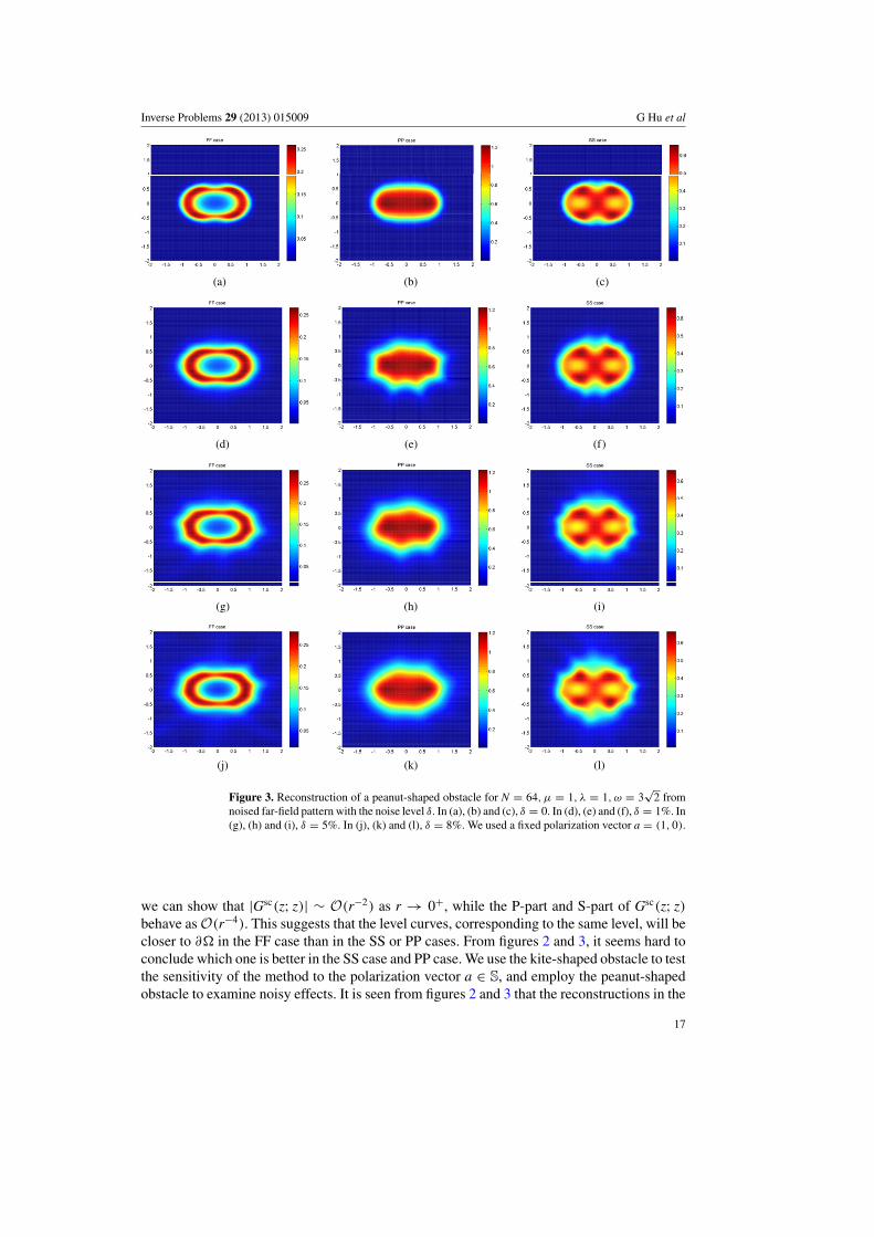
2 fromnoised far-field pattern with the noise level δ. In (a), (b) and (c), δ = 0. In (d), (e) and (f), δ = 1%. In(g), (h) and (i), δ = 5%. In (j), (k) and (l), δ = 8%. We used a fixed polarization vector a = (1, 0).
we can show that |Gsc(z; z)| ∼ O(r−2) as r → 0+, while the P-part and S-part of Gsc(z; z)behave as O(r−4). This suggests that the level curves, corresponding to the same level, will becloser to ∂� in the FF case than in the SS or PP cases. From figures 2 and 3, it seems hard toconclude which one is better in the SS case and PP case. We use the kite-shaped obstacle to testthe sensitivity of the method to the polarization vector a ∈ S, and employ the peanut-shapedobstacle to examine noisy effects. It is seen from figures 2 and 3 that the reconstructions in the
17

Inverse Problems 29 (2013) 015009 G Hu et al
SS case and PP case are more sensitive than the FF case to the polarization vector a and to thewhite noise of level δ.
It remains an interesting question to investigate the mixed PS case (resp. SP case), i.e.to reconstruct ∂� from the S-part (resp. P-part) of the far-field pattern corresponding to allincident plane pressure (resp. shear) waves. In our experiments, the F#-method fails if weapply the same inversion procedure to the SP or PS case. This is understandable, because thefactorization of the corresponding far-field operators in the mixed case (see (3.7) in the SS caseand (3.10) in the PP case) is no longer symmetric and thus the range identity of [17, Theorem2.15] is not applicable. A further investigation of these cases will be written in a future work.
Acknowledgments
The first author is financed by the German Research Foundation (DFG) under grant noEL 584/1-2. The third author is partially supported by the Austrian Science Fund (FWF):P22341-N18. This work was initiated when G Hu attended the Special Semester on MultiscaleSimulation & Analysis in Energy and the Environment (Workshop 3) held at RICAM, Linzin December 2011, and continued when he participated in the workshop Inverse Problemsfor Partial Differential Equations at the Mathematisches Forschungsinstitut Oberwolfach(MFO) in February 2012 and visited RICAM again in March 2012. The hospitality of the twoinstitutes and invitations from the organizers are greatfully acknowledged. The authors wouldalso like to thank Professor J Cheng for pointing out a mistake in section 2.2 of the originalversion.
Appendix
In this section, we give an explicit solution of the S-part of the scattered field for a ballD = BR := {|x| � R} in terms of radiating spherical vector wave functions and prove itsanalytical extension to R3\{0}. Let jn and yn be the spherical Bessel and Neumann functionsof order n, and recall that the linear combination h(1)
n := jn + i yn are known as sphericalHankel functions of the first kind of order n. In our calculations it is more convenient toemploy spherical coordinates. For x = (x1, x2, x3) ∈ R3, let r = |x|, x1 = r sin θ cos φ,x2 = r sin θ cos φ, x3 = r cos θ , and set
−→er = x := x/r,−→eθ := (cos θ cos φ, cos θ sin φ,− sin θ ),−→eφ := (− sin φ, cos φ, 0).
Suppose that uin is a plane wave to the Navier equation (1.1) in R3. Then there holds theexpansion
uin =∞∑
n=1
n∑m=−n
{Am
n
1
kp∇x[ jn(kpr)Y m
n (x)] + Bmn
1√n(n + 1)
curl x[x jn(ksr)Ym
n (x)]
+ Cmn
1√n(n + 1)ks
curl xcurl x[x jn(ksr)Ym
n (x)]
}(A.1)
for some constants Amn , Bm
n ,Cmn ∈ C, where Y m
n denote the spherical harmonics. The first termon the right hand side of (A.1) stands for the longitudinal mode, while the second and thirdterms represent the two transverse modes. Elementary calculations show that on |x| = R thereholds1
kp∇x
[jn(kpr)Y m
n (x)]|r=R = j′n(tp)Y
mn (x)x + jn(tp)
1
tpGradY m
n (x),
curlx[x jn(ksr)Y
mn (x)
]|r=R = jn(ts)GradY mn (x) × x,
18

Inverse Problems 29 (2013) 015009 G Hu et al
1
kscurlx curlx
[x jn(ksr)Y
mn (x)
]|r=R = n(n + 1)
tsY m
n (x)x + 1
ts
[jn(ts) + ts j′n(ts)
]GradY m
n (x),
where tp = kpR, ts = ksR and GradY mn := −→eθ ∂θY m
n + (sin θ )−1−→eφ ∂φY mn denotes the surface
gradient of Y mn over the unit sphere. Note that the tangential fields GradY m
n (x), GradY mn (x)× x
are called vector spherical harmonics of order n. Inserting the previous three identities into(A.1) gives
uin|r=R =∞∑
n=1
n∑m=−n
{[ j′n(tp)A
mn + t−1
s
√n(n + 1)Cm
n ]Y mn (x)x
+ 1√n(n + 1)
Bmn jn(ts) GradY m
n (x) × x
+[
t−1p jn(tp)A
mn + 1√
n(n + 1)ts( jn(ts) + ts j′n(ts))C
mn
]GradY m
n (x)
}. (A.2)
Since the scattered field usc = uscp + usc
s satisfies the radiation condition (1.8), the P-part uscp
and the S-part uscs can be expanded into
uscp =
∞∑n=1
n∑m=−n
Amn
1
kp∇x
[h(1)
n (kpr)Y mn (x)
],
uscs =
∞∑n=1
n∑m=−n
{Bm
n
1√n(n + 1)
curl x[xh(1)n (ksr)Y
mn (x)]
+ Cmn
1√n(n + 1) ks
curl xcurl x[xh(1)n (ksr)Y
mn (x)]
}for |x| � R with some complex valued constants Am
n , Bmn , Cm
n . On the surface |x| = R thescattered field usc admits an expansion analogous to (A.2) only with jn, Am
n , Bmn ,Cm
n replacedby h(1)
n , Amn , Bm
n , Cmn , respectively. Taking into account the Dirichlet boundary condition, we
obtain
Bmn h(1)
n (ts) = −Bmn jn(ts), Mn(tp, ts)
(Am
n
Cmn
)= −Mn(tp, ts)
(Am
nCm
n
), (A.3)
where Mn(tp, ts) is the 2 × 2 complex valued matrix given by
Mn(tp, ts) =(
h(1)n
′(tp) t−1s
√n(n + 1)
t−1p h(1)
n (tp)1
ts√
n(n+1)[h(1)
n (ts) + tsh(1)n
′(ts)]
)and Mn(tp, ts) is defined analogously to Mn(tp, ts) only with h(1)
n , h(1)n
′ replaced by jn, j′n.By the uniqueness of the forward elastic scattering problem, the above system (A.3) forAm
n , Bmn , Cm
n is uniquely solvable.Suppose that uin = uin
s is an incident plane shear wave taking the form (1.5). The vectoranalogue of the Jacobi–Anger expansion yields the expression (A.1) for uin
s with (see [20])
Amn = 0, Bm
n = −4π in√n(n + 1)
(d × GradY mn (d) · q),Cm
n = −4π in+1
√n(n + 1)
GradY mn (d) · q.
Consequently, we derive from (A.3) that
Bmn = in4π jn(kpR)√
n(n + 1)h(1)n (kpR)
(d × GradY mn (d) · q), Cm
n = Dmn
in+14π√n(n + 1)
GradY mn (d) · q,
with the coefficient
Dmn = fn(kpR) − [ jn(ksR) + ksR j′n(ksR)]
fn(kpR) − [h(1)n (ksR) + ksRh(1)
n′(ksR)]
, fn(kpR) := n(n + 1)h(1)n (kpR)
kpRh(1)n
′(kpR).
19

Inverse Problems 29 (2013) 015009 G Hu et al
Therefore we arrive at an explicit representation of the S-part uscs of usc with the coefficients
Bmn and Cm
n given above. By the addition theorem (see e.g. [6, theorem 2.8]) it can be furtherconcluded that usc
s is a function of cos β, where β denotes the angle between x and the incidentdirection d.
Since uscs satisfies the Maxwell equation, to prove its analytical extension into {x : |x| <
R, x = 0} we only need to justify the convergence of the tangential component of uscs in the
mean square sense on the sphere |x| = R0 for any 0 < R0 < R; see [6, theorem 6.26]. UsingParseval’s equality,∫
|x|=R0
|ν × uscs |2ds(x) = R2
0
∞∑n=1
n∑m=−n
|Bmn |2|h(1)
n (ksR0)|2
+ R20
∞∑n=1
n∑m=−n
{|Cmn |2 ∣∣h(1)
n′(ksR0) + (ksR0)
−1h(1)n (ksR0)
∣∣2}.
By the asymptotic behavior of the spherical Bessel and Hankel functions as n → ∞ and theirdifferential formulas (see e.g. [6, chapter 2.4] or [23]), we have
jn(t) = (2t)nn!
(2n + 1)!
(1 + O
(1
n
)),
t j′n(t) = n(2t)nn!
(2n + 1)!
(1 + O
(1
n
)),
h(1)n (t) = (2n − 1)!
i2n−1(n − 1)!tn
(1 + O
(1
n
)),
th(1)n
′(t) = − n(2n − 1)!
i2n−1(n − 1)!tn
(1 + O
(1
n
)).
Then we can check that indeed ||ν × uscs ||2L2(BR0 )3 < ∞ for any 0 < R0 < R.
References
[1] Alves C J and Kress R 2002 On the far-field operator in elastic obstacle scattering IMA J. Appl. Math. 67 1–21[2] Arens T 2001 Linear sampling method for 2D inverse elastic wave scattering Inverse Problems 17 1445–64[3] Athanasiadis C E, Sevroglou V and Statis I G 2008 3D elastic scattering theorem for point-generated dyadic
fields Math. Methods Appl. Sci. 31 987–1003[4] Charalambopoulos A, Kirsch A, Anagnostopoulos K A, Gintides D and Kiriaki K 2007 The factorization method
in inverse elastic scattering from penetrable bodies Inverse Problems 23 27–51[5] Colton D and Kirsch A 1996 A simple method for solving inverse scattering problems in the resonance region
Inverse Problems 12 383–93[6] Colton D and Kress R 1998 Inverse Acoustic and Electromagnetic Scattering Theory (Berlin: Springer)[7] Dassios G, Kiriaki K and Polyzos D 1987 On the scattering amplitudes for elastic waves J. Appl. Math. Phys.
38 855–73[8] Dassios G, Kiriaki K and Polyzos D 1995 Scattering theorems for complete dyadic fields Int. J. Eng.
Sci. 33 269–77[9] Elschner J and Yamamoto M 2010 Uniqueness in inverse elastic scattering with finitely many incident waves
Inverse Problems 26 045005[10] Gintides D, Sini M and Thanh N T 2012 Detection of point-like scatterers using one type of scattered elastic
waves J. Comput. Appl. Math. 236 2137–45[11] Gintides D and Sini M 2012 Identification of obstacles using only the scattered P-waves or the scattered S-waves
Inverse Problems Imaging 6 39–55[12] Hahner P and Hsiao G 1993 Uniqueness theorems in inverse obstacle scattering of elastic waves Inverse
Problems 9 525–34[13] Hu G, Liu X and Zhang B 2009 Unique determination of a perfectly conducting ball by a finite number of
electric far field data J. Math. Anal. Appl. 352 861–71
20

Inverse Problems 29 (2013) 015009 G Hu et al
[14] Ikehata M 1998 Reconstruction of the shape of the inclusion by boundary measurements Commun. Partial Diff.Eqns. 23 1459–74
[15] Isakov V 1990 On uniqueness in the inverse transmission scattering problem Commun. Partial Diff.Eqns. 15 1565–87
[16] Kirsch A 1998 Characterization of the shape of the scattering obstacle by the spectral data of the far-fieldoperator Inverse Problems 14 1489–512
[17] Kirsch A and Grinberg N 2008 The Factorization Method for Inverse Problems (Oxford Lecture Series inMathematics and its Applications vol 36) (Oxford: Oxford University Press)
[18] Kirsch A and Kress R 1993 Uniqueness in the inverse obstacle scattering problem Inverse Problems 9 285–99[19] Kress R 2002 Uniqueness in inverse obstacle scattering for electromagnetic waves Proc. URSI General Assembly
Maastricht[20] Kress R 2001 Electromagnetic waves scattering: scattering by obstacles Scattering ed R Pike and P Sabatier
(London: Academic Press) pp 175–210[21] Kupradze V D et al 1979 Three-Dimensional Problems of the Mathematical Theory of Elasticity and
Thermoelasticity (Amsterdam: North-Holland)[22] Martin P A and Dassios G 1993 Karp’s theorem in elastodynamic inverse scattering Inverse Problems 9 97–111[23] Monk P 2003 Finite Element Method for Maxwell’s Equations (Oxford: Oxford University Press)[24] Potthast R 1998 A point source method for inverse acoustic and electromagnetic obstacle scattering problems
IMA J. Appl. Math. 61 119–40[25] Sevroglou V 2005 The far-field operator for penetrable and absorbing obstacles in 2D inverse elastic scattering
Inverse Problems 21 717–38
21


![Technical Datasheet - Veracious Inc · Inverse Characteristics Curve [Over Current IDMT]: Very Inverse Long Inverse Standard Inverse Extremely Inverse α C 0.02 1 2 1 0.14 13.5 80](https://img.pdfslide.us/doc/110x75/60dab49f5dabad678957ab65/technical-datasheet-veracious-inc-inverse-characteristics-curve-over-current.jpg)