Some Exercises in

System Identification

Karl Henrik Johansson

Revised: Rolf Johansson

Maria Karlsson

Brad Schofield

Department of Automatic Control

Lund University

January 2007

Introduction to System Identification

1. This exercise is meant as an introduction to computer-based sys-

tem identification. We run an identification demonstration in Matlab.

Data from a laboratory scale hairdryer is used to estimate a model.

The demonstration includes several steps that will be discussed thor-

oughly later on in the course, so do not expect to understand all steps

taken in the demonstration.

Start

Matlab

Run the demonstration through the command

>> iddemo

and select demonstration 2) in the menu. Follow the information on

the screen.

When the demonstration is finished you end up in the menu. Select

1) and follow the demonstration of the graphical user interface. About

the same modeling is performed, but this time most Matlab commands

are hidden by the interface.

Test Signals

0 5 10 15 20 25 30

−1

−0.5

0

0.5

1

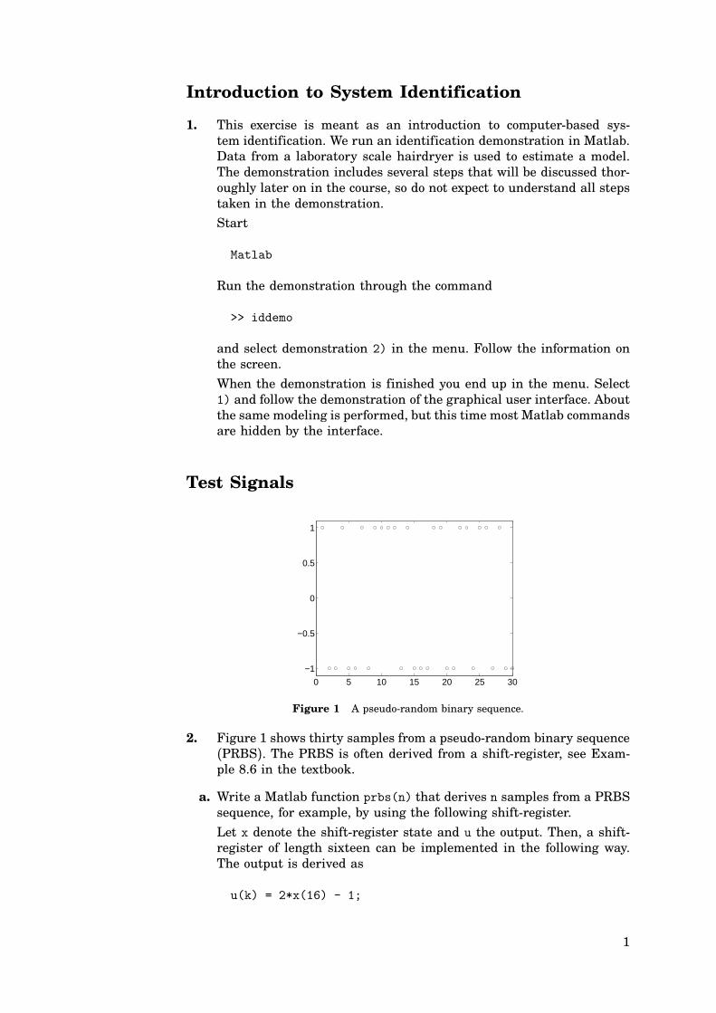
Figure 1 A pseudo-random binary sequence.

2. Figure 1 shows thirty samples from a pseudo-random binary sequence

(PRBS). The PRBS is often derived from a shift-register, see Exam-ple 8.6 in the textbook.

a. Write a Matlab function prbs(n) that derives n samples from a PRBS

sequence, for example, by using the following shift-register.

Let x denote the shift-register state and u the output. Then, a shift-

register of length sixteen can be implemented in the following way.

The output is derived as

u(k) = 2*x(16) - 1;

1

and then the states are updated as

d = x(16) + x(15) + x(13) + x(4);

x(2:16) = x(1:15);

x(1) = mod(d,2);

Draw a shift-register circuit corresponding to these equations, see

Figure 8.5 in the textbook.

b. If the period time of the shift-register is sufficiently long, its output

has approximately the same frequency content as white noise, that

is, the frequency spectrum is constant. Often in control applications

it is useful to have a test signal that has “white noise characteristics”

only up to a certain frequency, for example, the bandwidth of the

system. This can be conveniently implemented in the PRBS algorithm

by introducing the parameter period.

The PRBS in a could shift value every time the shift-register was

updated. Modify your Matlab function such that the output can only

shift value at time instances that are multiples of period. The function

should be called by the command prbs(n,period). Figure 2 shows

thirty samples from a PRBS with period = 3. Figure 1 correspondsto period = 1.

0 5 10 15 20 25 30

−1

−0.5

0

0.5

1

Figure 2 A pseudo-random binary sequence with period = 3.

c. Estimate and plot the frequency responses of the PRBS with various

values on period. There are dips in the spectra. How does the number

of dips relate to the parameter period?

Frequency Response Analysis

3. Consider a system

yk = G(q)uk + vkcontrolled by proportional feedback

uk = −Kyk

Derive a transfer function estimate G via discrete Fourier transfor-

mation of yk and uk and draw some conclusions?

2

4. Non-parametric identification results in a model given as a frequency

response, for example, a Bode plot. This type of identification it is often

useful to start with to get an idea of the process dynamics. However,

the parametric methods (for example, based on ARX or ARMAX mod-els) we discuss later on are more reliable and better suited for controldesign.

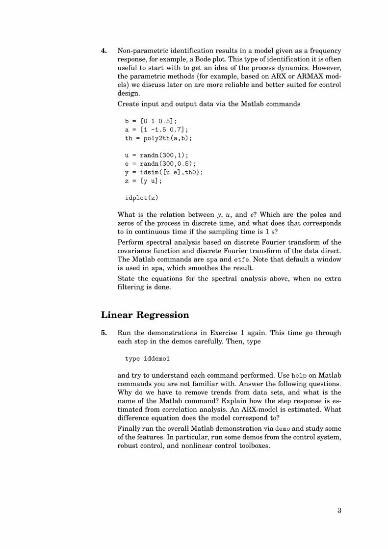
Create input and output data via the Matlab commands

b = [0 1 0.5];

a = [1 -1.5 0.7];

th = poly2th(a,b);

u = randn(300,1);

e = randn(300,0.5);

y = idsim([u e],th0);

z = [y u];

idplot(z)

What is the relation between y, u, and e? Which are the poles and

zeros of the process in discrete time, and what does that corresponds

to in continuous time if the sampling time is 1 s?

Perform spectral analysis based on discrete Fourier transform of the

covariance function and discrete Fourier transform of the data direct.

The Matlab commands are spa and etfe. Note that default a window

is used in spa, which smoothes the result.

State the equations for the spectral analysis above, when no extra

filtering is done.

Linear Regression

5. Run the demonstrations in Exercise 1 again. This time go through

each step in the demos carefully. Then, type

type iddemo1

and try to understand each command performed. Use help on Matlab

commands you are not familiar with. Answer the following questions.

Why do we have to remove trends from data sets, and what is the

name of the Matlab command? Explain how the step response is es-

timated from correlation analysis. An ARX-model is estimated. What

difference equation does the model correspond to?

Finally run the overall Matlab demonstration via demo and study some

of the features. In particular, run some demos from the control system,

robust control, and nonlinear control toolboxes.

3

Time-Series Analysis

6. Consider the system

S : yk = −ayk−1 + buk−1 + vk = ϕTk θ + vk

where v is a white noise sequence (not necessarily Gaussian). We areinterested in estimating the parameters a and b based on the data

y1, y2, . . . , yN and u1,u2, . . . ,uN .

a. Determine the loss function that is minimized for the maximum-

likelihood (ML) estimate, if vk has the density function

fv(vk) =1√2σe−√2pvkp/σ

b. Derive the least-squares (LS) estimate. What loss function is mini-mized?

c. Determine the loss function that is minimized for the ML estimate, if

vk is normal distributed and, hence,

fv(vk) =1√2πσ

e−v2k/2σ 2

Also, derive the estimate that minimizes the loss function.

d. What conclusions can be drawn?

7. Consider the system

S : yk + ayk−1 = b1uk−1 + b2uk−2 + vk

which is estimated with the instrument variable (IV) method usingdelayed inputs as instruments

zk =uk−1 uk−2 uk−3

T

Assume u is white Gaussian noise with zero mean and unit variance,

and that u and v are independent. Determine when the IV estimate

is consistent.

8. Consider the system

S : yk + a0yk−1 = uk

where u is zero mean white noise with variance λ2. We will examinetwo ways of predicting yk two steps ahead.

a. Let the model be

M1 : yk + ayk−1 = vkand estimate a. Then, the predictor is yk+2pk = a2yk. Derive the asymp-totic least-squares estimate of a and its variance.

4

b. Another way to get a two-step predictor is to consider the model

M2 : yk + β yk−2 = wk

and estimate β . The predictor is yk+2pk = −β yk. Derive the asymptoticleast-squares estimate of β . Show that w is not white noise by derivingits covariance function. (Hence, it is not possible to use the standardformula to calculate the variance of β . You do not have to derive thisvariance.)

c. Assume you have to choose one of the methods in a and b above in

order to predict yk two steps ahead. Discuss what criteria you would

consider to make your choice in a practical situation.

Model Validation and Reduction

9. Consider the system

S : yk+2 − yk+1 + 0.5yk = uk+1 − 0.5uk + ek+2

where ek ∈ N (0, 1). Let the input u be a PRBS signal with unitamplitude, and perform an identification experiment collecting 200

data points. Estimate AR(n,n)-models, that is,

M : yk+n + a1yk+n−1+ ⋅ ⋅ ⋅+ anyk = b0uk+n−1 + ⋅ ⋅ ⋅+ bn−1uk+ ek+n

where n = 1, . . . , 8. Derive and compare the loss function (the averageprediction error), Akaike’s information criterion and Akaike’s finalprediction error criterion of the models.

10. Consider the ARMA-system

S : yk = −ayk−1 + ek + cek−1

where {ek} is a white noise sequence with variance σ 2. Assume thatwe use the model

M : yk = −ayk−1 + ek + cek−1

and estimate a and c based on a prediction error method. Then it can

be shown that

θ ∈ AsN (θ , Cov(θ ))

where θ = a c

T is the prediction at time N and

Cov(θ ) = σ 2

N(c− a)2

$

(1− a2)(1− ac)2 (1− a2)(1− ac)(1− c2)(1− a2)(1− ac)(1− c2) (1− ac)2(1− c2)

5

“AsN ” denotes “asymptotically normal distributed,” so the distributionof θ will tend to be normal as N increases.

In the following subproblems we study how close a and c are. We see

from S that

yk =q+ cq+ a ek

so if a and c are sufficiently close the model reduces to yk = ek.

a. Determine the asymptotic variance of a− c.

b. Test the hypothesis

H 0 : a = con the significance level 0.05 based.

c. Do an F-test based on the two models

M1 : yk = ekM2 : yk + ayk−1 = ek + cek−1

and the hypotheses

H 0 : M1 is as good model for the system asM2

H 1 : M2 models the system better thanM1

that is,

H 0 : σ 21 = σ 22H 1 : σ 21 > σ 22

where σ 21 and σ 22 are the variances for the white noise ek in the modelM1 andM2, respectively. Can we reject H 0 on significance level 0.05?

11. We are interested in reducing the order of the model

Y(z) = z− 0.55(z− 0.5)(z− 0.8)U(z) (1)

Therefore we derive a balanced state-space model

xk+1 =0.7790 −0.0766−0.0766 0.5210

xk +

0.9884

0.1521

uk

yk =0.9884 0.1521

xk

The eigenvalues of the Gramians P and Q (see the textbook) are

σ 1

σ 2

=

2.4853

0.0517

Is it advisable to reduce the model order? If so, determine the reduced-

order model.

6

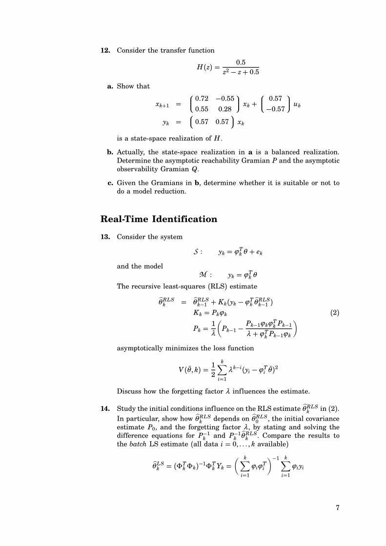
12. Consider the transfer function

H(z) = 0.5

z2 − z+ 0.5

a. Show that

xk+1 =0.72 −0.550.55 0.28

xk +

0.57

−0.57

uk

yk = 0.57 0.57

xk

is a state-space realization of H .

b. Actually, the state-space realization in a is a balanced realization.

Determine the asymptotic reachability Gramian P and the asymptotic

observability Gramian Q.

c. Given the Gramians in b, determine whether it is suitable or not to

do a model reduction.

Real-Time Identification

13. Consider the system

S : yk = ϕTkθ + ek

and the model

M : yk = ϕTk θ

The recursive least-squares (RLS) estimate

θ RLSk = θ RLSk−1 + Kk(yk −ϕTk θ RLSk−1 )Kk = Pkϕ k (2)

Pk =1

λ

(Pk−1 −

Pk−1ϕ kϕTk Pk−1λ +ϕT

kPk−1ϕ k

)

asymptotically minimizes the loss function

V (θ , k) = 12

k∑

i=1λ k−i(yi −ϕTi θ )2

Discuss how the forgetting factor λ influences the estimate.

14. Study the initial conditions influence on the RLS estimate θ RLSk in (2).In particular, show how θ RLSk depends on θ RLS0 , the initial covariance

estimate P0, and the forgetting factor λ , by stating and solving thedifference equations for P−1k and P−1k θ RLSk . Compare the results to

the batch LS estimate (all data i = 0, . . . , k available)

θ LSk = (ΦTkΦk)−1ΦTk Yk =( k∑

i=1ϕ iϕ

Ti

)−1 k∑

i=1ϕ iyi

7

Closed-Loop Identification

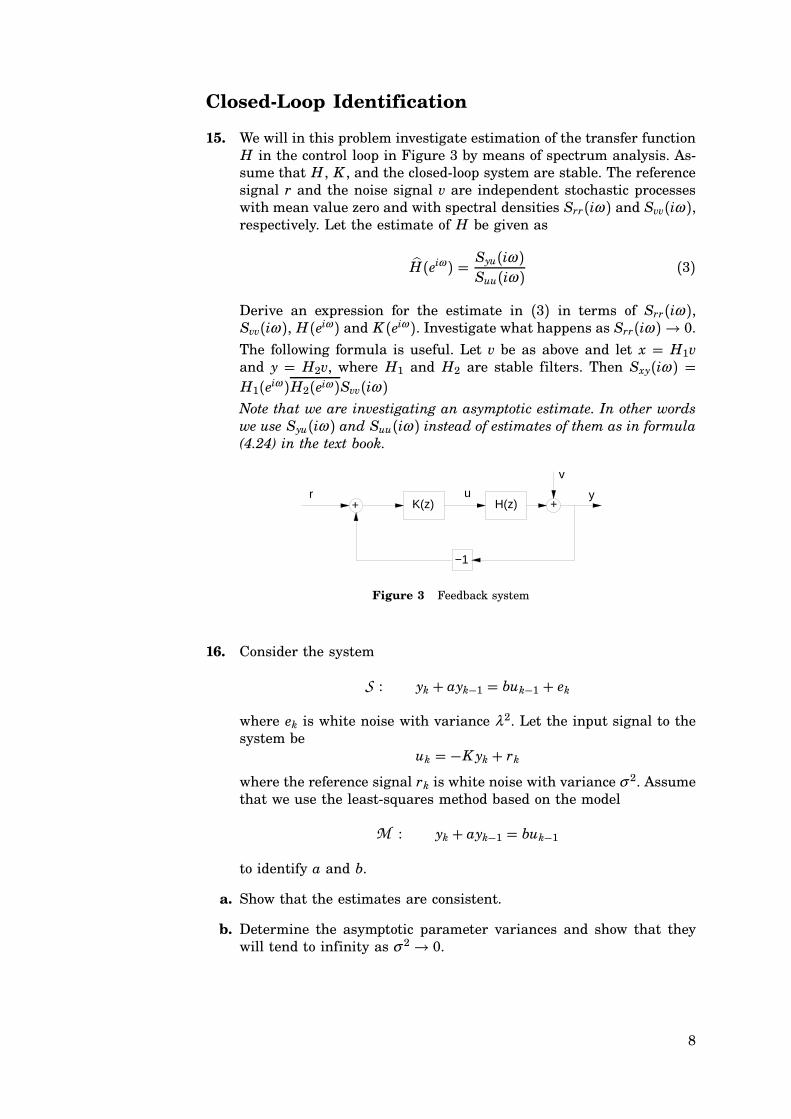
15. We will in this problem investigate estimation of the transfer function

H in the control loop in Figure 3 by means of spectrum analysis. As-

sume that H , K , and the closed-loop system are stable. The reference

signal r and the noise signal v are independent stochastic processes

with mean value zero and with spectral densities Srr(iω ) and Svv(iω ),respectively. Let the estimate of H be given as

H(eiω ) = Syu(iω )Suu(iω )

(3)

Derive an expression for the estimate in (3) in terms of Srr(iω ),Svv(iω ), H(eiω ) and K (eiω ). Investigate what happens as Srr(iω ) → 0.The following formula is useful. Let v be as above and let x = H1vand y = H2v, where H1 and H2 are stable filters. Then Sxy(iω ) =H1(eiω )H2(eiω )Svv(iω )Note that we are investigating an asymptotic estimate. In other words

we use Syu(iω ) and Suu(iω ) instead of estimates of them as in formula(4.24) in the text book.

−1

H(z)K(z)+u yr

+

v

Figure 3 Feedback system

16. Consider the system

S : yk + ayk−1 = buk−1 + ek

where ek is white noise with variance λ2. Let the input signal to thesystem be

uk = −Kyk + rkwhere the reference signal rk is white noise with variance σ 2. Assumethat we use the least-squares method based on the model

M : yk + ayk−1 = buk−1

to identify a and b.

a. Show that the estimates are consistent.

b. Determine the asymptotic parameter variances and show that they

will tend to infinity as σ 2 → 0.

8

17. Consider the unstable first-order process

S : yk + ayk−1 = buk−1 + ek, Ee2k = λ2

Our model is

M : yk + ayk−1 = buk−1The process is controlled by a proportional controller chosen such that

the closed-loop system is stable. To the control signal an external

signal is added to excite the system, hence,

uk = − f yk + vk, Ev2k = σ 2

The stochastic processes e and v are independent white noises with

means equal to zero. Which one of the following two methods gives

best accuracy?

1. Measure u and y. Derive least-squares estimates of a and b.

2. Measure v and y. Derive a least-squares estimate of the closed-

loop system. Out of this estimate, calculate the estimates of a

and b.

Hint: Recall from the Computer-Controlled Systems course that for a

first-order system

yk =b0q+ b1a0q+ a1

uk

the variance of yk is

Ey2k =(b20 + b21)a0 − 2b0b1a1

a0(a20 − a21)Eu2k

Subspace Identification

18. In this exercise, we will investigate the use of state-space model iden-

tification.

In particular, subspace-based methods will be introduced. As prepa-

ration, read Chapter 13 and Appendix E in System Modeling and

Identification Exercises We will use Matlab software throughout the

exercise. Begin by installing the SMI-1.0 toolbox, available at:

• http://www.control.lth.se/~FRT041/local/smi1_0d.tgz

Download the SMI Toolbox Manual:

• http://www.control.lth.se/~FRT041/local/smimanual-1.0.pdf

The SMI-1.0 toolbox implements the Multivariable Output-Error State

Space (MOESP) class of state space algorithms. Read through themanual, and run through the examples in Chapter 5. Try to identify

some parametric models using the data from the examples. Compare

their performance with that of the state space models given by the

9

MOESP algorithms using some common measure. The Matlab com-

mand n4sid uses subspace methods to identify state space models.

Acquaint yourself with the use of the command, and try to identify

some models using the data from the SMI toolbox manual examples.

Compare the performance with the SMI toolbox algorithms and with

other parametric models. Subspace algorithms may be directly applied

to multivariable systems. Investigate this by using the rss command

in Matlab to generate random state space systems of a given order

and input/output dimensions, and trying to identify the system. Whatcan be said about the use of parametric identification for multivari-

able systems?

Finally, download the identification data:

• http://www.control.lth.se/~FRT041/data.zip

and use state-space identification methods to obtain a model.

10

Solutions

Introduction to System Identification

1.

Test Signals

2.

a. See the solution in b.

b. function u = prbs(n,period);

% PRBS Pseudo random binary sequence

%

% u = prbs(n,period) gives a PRBS row vector of

% length n. The sequence periodiod has length

% 2^16-1. period is the same variable as in the

% computer program logger (default 1).

u = zeros(n,1);

x = [zeros(1,15) 1]; % Initial state

if nargin==1,

period = 1;

end

p = period;

for k = 1:n,

if p == period,

p = 1;

u(k) = 2*x(16) - 1;

d = x(16) + x(15) + x(13) + x(4);

x(2:16) = x(1:15);

x(1) = mod(d,2);

else

u(k) = u(k-1);

p = p + 1;

end

end;

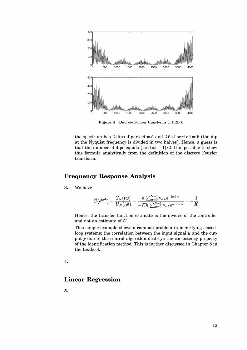
c. The Matlab function fft derives the discrete Fourier transform of a

vector. The following commands gives the plots in Figure 4:

n=2^12;

p1=5;

p2=6;

plot(abs(fft(prbs(n,p1))));

plot(abs(fft(prbs(n,p2))));

Notice that the point 2048 on the x-axis corresponds to the Nyquist

frequency (corresponding to the end of the spectrum). We see that

11

0 500 1000 1500 2000 2500 3000 3500 40000

100

200

300

400

0 500 1000 1500 2000 2500 3000 3500 40000

100

200

300

400

Figure 4 Discrete Fourier transforms of PRBS.

the spectrum has 2 dips if period = 5 and 2.5 if period = 6 (the dipat the Nyquist frequency is divided in two halves). Hence, a guess isthat the number of dips equals (period− 1)/2. It is possible to showthis formula analytically from the definition of the discrete Fourier

transform.

Frequency Response Analysis

3. We have

G(eiωh) = YN(iω )UN(iω )

= h∑N−1m=0 ymhe

−iωhm

−Kh∑N−1m=0 ymhe

−iωhm= − 1

K

Hence, the transfer function estimate is the inverse of the controller

and not an estimate of G.

This simple example shows a common problem in identifying closed-

loop systems; the correlation between the input signal u and the out-

put y due to the control algorithm destroys the consistency property

of the identification method. This is further discussed in Chapter 8 in

the textbook.

4.

Linear Regression

5.

12

Time-Series Analysis

6.

a. The likelihood function to be maximized is

L(θ ) = P(ε pθ ) = fε (ε 2, . . . , ε N pθ ) = fv(ε 2, . . . , ε N) =N∏

k=2fv(ε k)

where fε is the density function of the residuals ε k = yk − ϕTk θ , andθ is assumed to be the true estimate. Notice that we have used thatsince v is white noise,

fv(v2, . . . ,vN) =N∏

k=2fv(vk)

Further,

log L(θ ) = −(N − 1) log(√2σ ) −

√2

σ

N∑

k=2pε kp

Hence, the loss function to be minimized is

J(a, b) =N∑

k=2pyk − (−ayk−1 + buk−1)p

b. The LS estimate is

θ = (ΦTΦ)−1ΦTY

=

∑Nk=2 y

2k−1 −∑N

k=2 yk−1uk−1

−∑Nk=2 yk−1uk−1

∑Nk=2 u

2k−1

−1

−∑N

k=2 ykyk−1∑Nk=2 ykuk−1

(4)

It minimizes the loss function

J(a, b) =N∑

k=2(yk − (−ayk−1 + buk−1))2 (5)

c. In the case of normal distributed noise v, we redo the calculations in

Section 6.3 in the textbook. Then, the loss function becomes identical

to (5). Hence, the estimate is the same as in (4).

d. In the case of white Gaussian (normal distributed) noise, we concludethat the LS estimate is the optimal estimate. If the noise is not Gaus-

sian, the LS estimate is usually not optimal. Further, if the white

noise assumption is violated, then the ML estimate is different from

the LS estimate even if the noise is normal distributed.

13

7. We have the system

S : Y = Φθ + Vand the model

M : Y = Φθ (6)where

Φ =

ϕT4...

ϕTN

=

−y3 u3 u2...

...

−yN−1 uN−1 uN−2

and

θ = a b1 b2

T V =

v4 . . . vN

T

By multiplying left- and right-hand side of (6) with

Z =

zT4...

zTN

we get the IV estimate

θ = (ZTΦ)−1ZTY = θ + (ZTΦ)−1ZTV

Hence, the estimate is consistent if E{zkϕTk } is non-singular and z isuncorrelated with v. We have

ZTΦ =

u3 . . . uN−1u2 . . . uN−2u1 . . . uN−3

T

−y3 u3 u2...

...

−yN−1 uN−1 uN−2

=

−∑N−13 ukyk

∑N−13 u2k

∑N−13 ukuk−1

−∑N−13 uk−1yk

∑N−13 uk−1uk

∑N−13 u2k−1

−∑N−13 uk−2yk

∑N−13 uk−2yk

∑N−13 uk−2uk−1

Thus,

E{zkϕTk } = limN→∞

1

N − 3ZTΦ =

0 1 0

−E{ukyk+1} 0 1

−E{ukyk+2} 0 0

where

E{ukyk+1} = E{uk(−ayk + b1uk + b2uk−1 + vk+1) = b1E{ukyk+2} = E{uk(−a(yk + b1uk + b2uk−1 + vk+1) + b1uk+1 + b2uk + vk+2)

= −ab1 + b2

so that E{ZTΦ} is non-singular if

det E{zkϕTk } = b2 − ab1 ,= 0

14

Notice that the transfer function from u to y given by S is

b1q+ b2q(q+ a)

The equality b2−ab1 = 0 is equal to a pole-zero cancellation in S , andis thus a degenerated case. Finally, since z and v are uncorrelated, we

conclude that the IV estimate is consistent.

8.

a. We have

a =(

ΦTNΦN

)−1ΦTNY N →

(Ey2k−1

)−1(−Eykyk−1)

=(

λ2

1− a20

)−1a0λ

2

1− a20= a0

and

Var a = λ2(

ΦTNΦN

)−1→ λ2

N

(Ey2k−1

)−1= 1− a

20

N

b. It holds that

β =(

ΦTNΦN

)−1ΦTNY N →

(Ey2k−2

)−1(−Eykyk−2)

=(

λ2

1− a20

)−1 −a20λ21− a20

= −a20

From S , we haveyk − a2oyk−2 = uk + a0uk−1

and since β is an unbiased estimate, asymptotically

wk = uk + a0uk−1

Hence, the covariance function

Cww(τ ) =

(1+ a20)λ2, τ = 0−a0λ2, pτ p = 10, pτ p ≥ 2

c. It is reasonable to choose the predictor yk+2pk minimizing qyk+2 −yk+2pkq. Depending on the choice of norm q ⋅ q, this problem can behard to solve analytically.

In our case, both estimates a2 and β are asymptotically unbiased.However, in a practical situation the data sequences have a limit

length. Therefore, it is interesting to study how fast these estimates

and their variances converge.

15

Model Validation and Reduction

9. Let p = 2n denote the number of parameters in the modelsM and N

the number of data points. The loss function

V (θ) = 1N

N∑

k=1

1

2ε 2k(θ ), ε k(θ ) = yk −ϕTk θ

the Akaike information criterion

AIC(p) = log V (θ ) + 2pN

and the final prediction error criterion

FPE(p) = N + pN − pV (θ )

are derived in Matlab by the following commands.1

% System ----------------------------------

a_true=poly([0.5+0.5i,0.5-0.5i]);

b_true=[0 1 -0.5];

% a_true =

% 1.0000 -1.0000 0.5000

% b_true =

% 0 1.0000 -0.5000

th_true=poly2th(a_true,b_true);

% Identification experiment ---------------

N=200;

u=prbs(N);

randn(’seed’,2)

e=randn(N,1);

y=idsim([u e],th_true);

% Model estimation ------------------------

NN=[ 1 1 1; % Model structure [na nb nk]

2 2 1;

3 3 1;

4 4 1;

5 5 1;

6 6 1;

7 7 1;

8 8 1;];

M=arxstruc([y(1:N) u(1:N)],[y(1:N) u(1:N)],NN);

% Criteria calculation --------------------

1The commands prbs and akaike are not included in standard Matlab packages.

16

0 2 4 6 8 10 12 14 16 180.8

11.21.41.6

Loss function

0 2 4 6 8 10 12 14 16 180

0.2

0.4

Akaike’s information criterion

0 2 4 6 8 10 12 14 16 181

1.2

1.4

1.6

# parameters

Akaike’s final prediction error criterion

Figure 5 Loss function, AIC, and FPE in Exercise 4.

V=M(1,1:size(M,2)-1); % The loss function

[aic,fpe]=akaike(V,NN,N); % AIC and FPE

Figure 5 shows V , AIC, and FPE as functions of the number of esti-

mated parameters p. We note that the loss function is a monotonously

decreasing function, whereas both AIC and FPE has a minimum for

p = 4 (the latter one is however hard to see). Hence, in this example,minimizing AIC or FPE gives a model with a number of parameters

equal to the number in the system.

10.

a. The variance is

Var(a− c) = Var( 1 −1

θ ) =

1 −1

Cov(θ )

1

−1

= 1− a2c2

N

b. From a we know that under H 0 it holds that

a− c ∈ AsN (0,µ2), µ2 = 1− a2c2

N

Introduce the normalized stochastic variable

X = a− cµ

= a− b√1−a2c2N

∈ AsN (0, 1)

From the statistic course, we know that

P(pX p > λα /2) = α

17

where α is the probability that the null hypothesis is rejected if it istrue, and λα /2 can be found in statistic tables.

λ

α/2

α/2

Hence, reject H 0 (on significance level α ) if

pa− cp > λα /2

√1− a2c2N

For α = 0.05 we have λα /2 = 1.96.

c. F-tests are discussed in Section 9.3, B.3, and B.5 in the textbook.

Notice that these tests are performed under the assumption that a

correct model (under a certain hypothesis) gives optimal predictionerrors ε k, that is, ε k = ek.Let V1 and V2 denote the sum of the squared residuals for the two

models, and p1 = 0 and p2 = 2 the number of estimated parameters.Then, under the hypothesis H 0,

Vi

σ 2=

N∑

k=pi+1

ε ikσ 2

∈ χ 2(N − pi), i = 1, 2

where N − pi is called the degree of freedom. Taking the differencebetween V1 and V2 (under the assumption that the prediction errorsare optimal), it follows that the degree of freedom reduces to p1 − p2,so that

(V1 − V2)/σ 2 ∈ χ 2(p2 − p1)The quotient of two χ 2-distributed variables is F-distributed. We haveunder H 0 that

V1 − V2V2

⋅N − p2p2 − p1

∈ F(p2 − p1,N − p2)

Let Fα denote the α -percentile. Then, we reject H 0 if

V1 − V2V2

⋅N − 22

> Fα (2,N − 2)

α

F (f ,f )α 1 2

There is a probability α that H 0 is rejected even if it is true. Fα (2,N−2) is given in tables. For instance, for α = 0.05 we have

limN→∞

Fα (2,N − 2) = 2.60

18

11. A balanced realization has similar properties of reachability and ob-

servability. The magnitude of the elements of the Gramian expresses

the relative importance of each state. Since σ 1 ≫ σ 2, the second statehas low influence on the input-output behavior. Therefore, it seems

advisable to reduce the model to a first order model. We eliminate the

second state, so that x(2)k+1 = x

(2)k. This gives the following equation for

x(2)

x(2)k = −0.0766x(1)k + 0.5210x(2)k + 0.1521uk

Solving for x(2) and substituting in the state space model gives thereduced order state-space model

xk+1 = 0.7912xk + 0.9641ukyk = 0.9641xk + 0.0483uk

The transfer function for this model is

Hred(z) =0.0483z+ 0.8912z− 0.7912

Since

Hred(z) (0.9

z− 0.8the reduction is almost a pole-zero cancellation. However, we have

to be careful; not all “almost pole-zero cancellation” should be done

(compare exercise 10.2 in the textbook).

12.

a. For the given state-space realization {Φ,Γ,C}, direct calculations give

C(zI − Φ)−1Γ = H(z)

b. For a balanced realization, the asymptotic reachability Gramian P is

equal to the asymptotic observability Gramian Q. The diagonal matrix

Σ = P = Q fulfills the discrete-time Lyapunov equations

ΦΣΦT − Σ + ΓΓT = 0

ΦTΣΦ − Σ + CTC = 0

Solving the first equation gives

Σ = P = Q =1.12 0

0 0.72

A check gives that also the second Lyapunov equation is fulfilled.

c. Since the elements in the Gramians do not vary with a factor of mag-

nitude, it is not suitable to perform a state reduction. (Notice that Hhas complex poles.)

19

Real-Time Identification

13. The forgetting factor λ ∈ (0, 1] is typically chosen between 0.97 and0.995. Its value should reflect the time-variation in the process. A

forgetting factor λ = 1 gives that all data points are weighted equally,and is, hence, the theoretical choice for a time-invariant process. From

the Taylor expansion around λ = 1

ln(1+ (λ − 1)) = (λ − 1) + . . .

we get

λ k−i = e(k−i) ln λ ( e−(k−i)(1−λ) = e−(k−i)/T

where T = 1/(1 − λ) is the time constant defining the approxi-mate number of samples included in V . The suggested choice λ ∈[0.97, 0.995] corresponds to T ∈ [33, 200]. Roughly, there is no influ-ences from data older than 2T .

14. In the batch LS problem we consider the matrix

Pk = (ΦTkΦk)−1 =( k∑

i=1ϕ iϕ

Ti

)−1

It satisfies the recursive equation

P−1k = P−1k−1 +ϕ kϕTk

We get the corresponding RLS covariance matrix by including the

forgetting factor:

P−1k = λP−1k−1 +ϕ kϕTk

with initial value P0. The solution is

P−1k = λ kP−10 +k∑

i=1λ k−iϕ iϕ

Ti (7)

Further, P−1k θ RLSk satisfies

P−1k θ RLSk = P−1k θ RLSk−1 + P−1k Kk(yk −ϕTk θ RLSk−1 )= λP−1k−1θ

RLSk−1 +ϕ kϕ

Tk θ RLSk−1 +ϕ kyk −ϕ kϕ

Tk θ RLSk−1

= λP−1k−1θRLSk−1 +ϕ kyk

so that

P−1k θ RLSk = λ kP−10 θ RLS0 +k∑

i=1λ k−iϕ iyi (8)

From (7) and (8), we have

θ RLSk =(

λ kP−10 +k∑

i=1λ k−iϕ iϕ

Ti

)−1(λ kP−10 θ RLS0 +

k∑

i=1λ k−iϕ iyi

)

Hence,

20

• If λ < 1, the influences of initial conditions tend to zero as k→∞.

• If λ = 1 and P0 = ρ I, then the influences of initial conditionstend to zero as ρ →∞.

• If λ = 1, then

θ RLSk − θ LSk = Pk(λ kP−10 θ RLS0 +k∑

i=1λ k−iϕ iyi) − PkP−1k θ LSk

= Pk

(P−10 θ RLS0 +

k∑

i=1ϕ iyi − (P−10 +

k∑

i=1ϕ iϕ

Ti )θ LSk

)

= Pk(P−10 θ RLS0 − P−10 θ LSk ) = PkP−10 (θ RLS0 − θ LSk )

Thus,

limPk→0

θ RLSk − θ LSk = 0

Further, by differentiating the loss function

V (θ) = (θ − θ0)TP−10 (θ − θ0) + ε Tε (9)

where ε = Y − Φθ , we get

dV

dθ= −Y TΦ + θTΦTΦ + (θ − θ0)TP−10 = 0

for θ = θ RLS. Hence, minimizing the loss function (9) gives a batchestimate equal to the RLS estimate with λ = 1.

Closed-Loop Identification

15. We have

u = K

1+ KH (r − v)

y = 1

1+ HK v+HK

1+ HK r

and since r and v are independent, we get

Suu(iω ) =pK (eiω )p2

p1+ H(eiω )K (eiω )p2 (Srr(iω ) + Svv(iω ))

Syu(iω ) =H(eiω )pK (eiω )p2

p1+ H(eiω )K (eiω )p2 Srr(iω ) −K (eiω )

p1+ H(eiω )K (eiω )p2 Svv(iω )

The estimate is

H(eiω ) = H(eiω ) − H(eiω )K (eiω ) + 1K (eiω )

Svv(iω )Svv(iω ) + Srr(iω )

and as Srr(iω ) → 0, we get

H(eiω ) → − 1

K (eiω )

21

16. The model is given by

M : yk =−yk−1 uk−1

a

b

= φTkθ

so that we obtain the estimates as

θ = (ΦTΦ)−1ΦTY

where

Φ =

−y1 u1...

...

−yN−1 uN−1

Y =

y2...

yN

a. We have that Y = Φθ +E. This gives

θ = θ + ( 1N

ΦTΦ)−1( 1N

ΦTE) → θ , N →∞

since interacting elements of Φ and E are uncorrelated.

b. Using the central limit theorem (eq. 6.89), we have that

√N(θ − θ ) ∈ AsN (0,Σ), Σ = λ2E( 1

NΦTΦ)−1

which gives

Cov(θ ) = 1N

Σ = λ2

NlimN→∞

(1

N

∑y2k −∑

ykuk

−∑ykuk

∑u2k

)−1

Deriving the asymptotic diagonal elements gives

Var(a) = λ2

N

ru(0)ry(0)ru(0) − r2yu(0)

Var(b) = λ2

N

ry(0)ry(0)ru(0) − r2yu(0)

Introduce α = a+Kb to simplify further calculations. Using the closedloop system

S : yk = −(a+ Kb)yk−1 + brk−1 + ek

and some calculations we obtain

ry(0) =b2σ 2 + λ2

1−α 2ru(0) = σ 2 + K 2ry(0) ryu(0) = −Kry(0)

so that

Var(a) = λ2

N

(K 2

σ 2+ 1−α 2

b2σ 2 + λ2

)Var(b) = λ2

N⋅1

σ 2

From these expressions we observe that the asymptotic parameter

variances will tend to infinity if σ → 0.

22

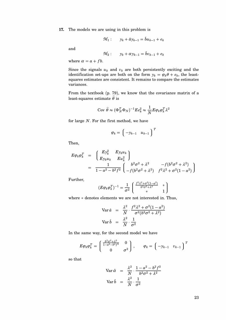
17. The models we are using in this problem is

M1 : yk + ayk−1 = buk−1 + ek

and

M2 : yk +α yk−1 = bvk−1 + ekwhere α = a+ f b.

Since the signals uk and vk are both persistently exciting and the

identification set-ups are both on the form yk = ϕ kθ + ek, the least-squares estimates are consistent. It remains to compare the estimates

variances.

From the textbook (p. 79), we know that the covariance matrix of aleast-squares estimate θ is

Cov θ ( (ΦTNΦN)−1Ee2k (1

NEϕ kϕ

Tk λ2

for large N . For the first method, we have

ϕ k =−yk−1 uk−1

T

Then,

Eϕ kϕTk =

Ey2k Eykuk

Eykuk Eu2k

= 1

1− a2 − b2 f 2

b2σ 2 + λ2 − f (b2σ 2 + λ2)− f (b2σ 2 + λ2) f 2λ2 +σ 2(1− a2)

Further,

(Eϕ kϕTk )−1 =

1

σ 2

f 2λ2+σ 2(1−a2)b2σ 2+λ2 ∗

∗ 1

where ∗ denotes elements we are not interested in. Thus,

Var a = λ2

N⋅f 2λ2 +σ 2(1− a2)

σ 2(b2σ 2 + λ2)

Var b = λ2

N⋅1

σ 2

In the same way, for the second model we have

Eϕ kϕTk =

b2σ 2+λ2

1−a2−b2 f 2 0

0 σ 2

, ϕ k =

−yk−1 vk−1

T

so that

Var α = λ2

N⋅1− a2 − b2 f 2b2σ 2 + λ2

Var b = λ2

N⋅1

σ 2

23

Hence, the estimate of b is as good in the first method as in the second.

In the second method, a is derived from α . Then,

Var a = Var α + f 2 Var b− 2 fCov (α , b) = λ2

N

(1− a2 − b2 f 2b2σ 2 + λ2

+ f2

σ 2

)

= f 2λ2 +σ 2(1− a2)σ 2(b2σ 2 + λ2)

which is identical to the variance in the first method. To conclude,

in this case it does not matter if the identification is done in open or

closed loop.

24