Matlab Exercises - University of New South WalesMatlab Exercises 2 1 Matlab Exercises for Chapter 1 % Matlab exercises for Chapter 1 % The following codes provide some exercises or

Matlab Exercises 1

Matlab

Exercises

1 Matlab Exercises for Chapter 1 ............................................... 2

2 Matlab Exercises for Chapter 2 ............................................... 7

3 Matlab Exercises for Chapter 3 ............................................. 10







Matlab Exercises 2

1 Matlab Exercises for Chapter 1

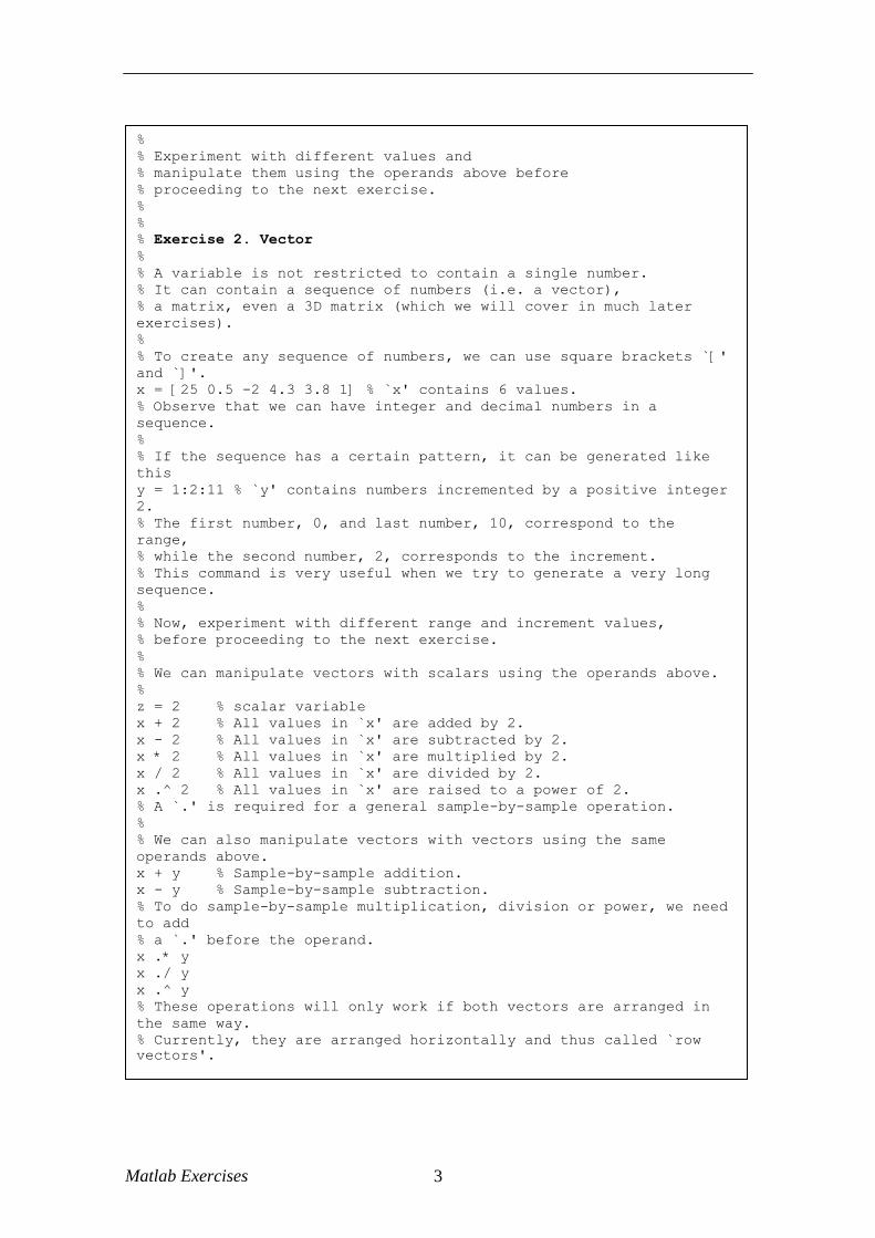
% Matlab exercises for Chapter 1

%

% The following codes provide some exercises or demonstrations

% which students may run in Matlab.

% The purpose of these exercises is to learn using Matlab for

% signal processing simulation.

%

% The best way to run this exercise is to copy and paste each

% Matlab command to the Matlab command window and then observe

% the results.

% However, it is also possible to run the entire exercise.

% To do so from the Matlab command windos, go to `File' and choose

`Run script'.

% Type the filename (which has .m extension) or use the browse

% button to find the file.

% To run the m-file from Matlab editor, go to `Tools' and choose

`Run'.

%

% By the end of the exercises, students should be able to

% - generate scalars and vectors in Matlab

% - manipulate scalars and vectors

% - plot vectors

% - generate unit step and impulse functions

% - generate cosine and sine functions

%

% Note:

% Matlab works with discrete-time signals (i.e. sequences of

numbers),

% not continuous-time signals.

% However, as we shall see shortly, we can generate an

% approximately continous-time signals.

%

%

%

% Exercise 1. Scalar (single value)

%

% We first create a variable called `x' which contains a number.

% The command to do this is

x = 10 % `x' now contains a value 10.

% We can also generate a decimal number.

y = 0.5 % `y' contains a value 0.5.

% We can manipulate these variables using the following operands.

x + y % adding the two variables.

%The outcome is stored in a temporary variable àns'.

x - y % subtracting `y' from `x'.

x * y % multiplying `x' and `y'.

x / y % dividing `x' and `y'.

x ^ y % raising `x' to the power of `y'.

%

% We can also change the value inside these variables,

% simply by replacing them with new values.

x = 5.5 % `x' now contains a value 5.5.

y = 2 % `y' now contains a value 2.

Matlab Exercises 3

%

% Experiment with different values and

% manipulate them using the operands above before

% proceeding to the next exercise.

%

%

% Exercise 2. Vector

%

% A variable is not restricted to contain a single number.

% It can contain a sequence of numbers (i.e. a vector),

% a matrix, even a 3D matrix (which we will cover in much later

exercises).

%

% To create any sequence of numbers, we can use square brackets `['

and `]'.

x = [25 0.5 -2 4.3 3.8 1] % `x' contains 6 values.

% Observe that we can have integer and decimal numbers in a

sequence.

%

% If the sequence has a certain pattern, it can be generated like

this

y = 1:2:11 % `y' contains numbers incremented by a positive integer

2.

% The first number, 0, and last number, 10, correspond to the

range,

% while the second number, 2, corresponds to the increment.

% This command is very useful when we try to generate a very long

sequence.

%

% Now, experiment with different range and increment values,

% before proceeding to the next exercise.

%

% We can manipulate vectors with scalars using the operands above.

%

z = 2 % scalar variable

x + 2 % All values in `x' are added by 2.

x - 2 % All values in `x' are subtracted by 2.

x * 2 % All values in `x' are multiplied by 2.

x / 2 % All values in `x' are divided by 2.

x .^ 2 % All values in `x' are raised to a power of 2.

% A `.' is required for a general sample-by-sample operation.

%

% We can also manipulate vectors with vectors using the same

operands above.

x + y % Sample-by-sample addition.

x - y % Sample-by-sample subtraction.

% To do sample-by-sample multiplication, division or power, we need

to add

% a `.' before the operand.

x .* y

x ./ y

x .^ y

% These operations will only work if both vectors are arranged in

the same way.

% Currently, they are arranged horizontally and thus called `row

vectors'.

Matlab Exercises 4

% We can arrange them vertically, i.e. `column vectors', by

transposing them.

x = x' % `x' is now transposed and become a column vector.

%

% Now, try applying the operations above between `x' and `y'.

% We will see that an error message will appear.

%

% To display a particular sample in a vector, use brackets `(' and

`)'.

x(3) % displays the third sample of vector `x'.

y(5) % displays the fifth sample of vector `y'.

%

% Specifiying a zero or negative value inside the bracket will

produce an

% error message. Try this.

%

% Furthermore, we can also display a subset of the vectors.

x(2:4) % displays the second to fourth samples.

y(3:2:5) % displays the third and fifth samples.

%

%

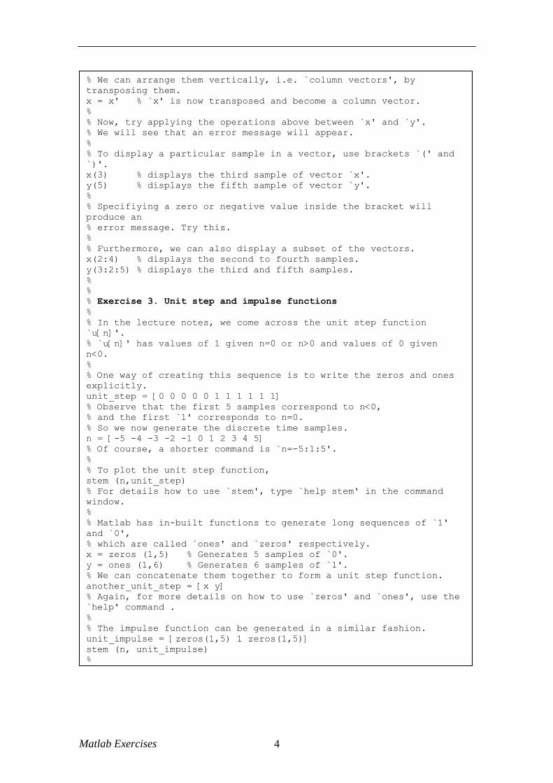
% Exercise 3. Unit step and impulse functions

%

% In the lecture notes, we come across the unit step function

ù[n]'.

% ù[n]' has values of 1 given n=0 or n>0 and values of 0 given

n<0.

%

% One way of creating this sequence is to write the zeros and ones

explicitly.

unit_step = [0 0 0 0 0 1 1 1 1 1 1]

% Observe that the first 5 samples correspond to n<0,

% and the first `1' corresponds to n=0.

% So we now generate the discrete time samples.

n = [-5 -4 -3 -2 -1 0 1 2 3 4 5]

% Of course, a shorter command is `n=-5:1:5'.

%

% To plot the unit step function,

stem (n,unit_step)

% For details how to use `stem', type `help stem' in the command

window.

%

% Matlab has in-built functions to generate long sequences of `1'

and `0',

% which are called ònes' and `zeros' respectively.

x = zeros (1,5) % Generates 5 samples of `0'.

y = ones (1,6) % Generates 6 samples of `1'.

% We can concatenate them together to form a unit step function.

another_unit_step = [x y]

% Again, for more details on how to use `zeros' and ònes', use the

`help' command .

%

% The impulse function can be generated in a similar fashion.

unit_impulse = [zeros(1,5) 1 zeros(1,5)]

stem (n, unit_impulse)

%

Matlab Exercises 5

-5 0 5 10 150

0.5

1unit step

-5 0 5 10 150

0.5

1unit step shifted left

-5 0 5 10 150

0.5

1unit step shifted right

-5 0 5 10 150

0.5

1y

0 2 4 6 8 10 12 14 16 18 200

0.1

0.2

0.3

0.4

0.5

0.6

0.7

0.8

0.9

1alphan

%

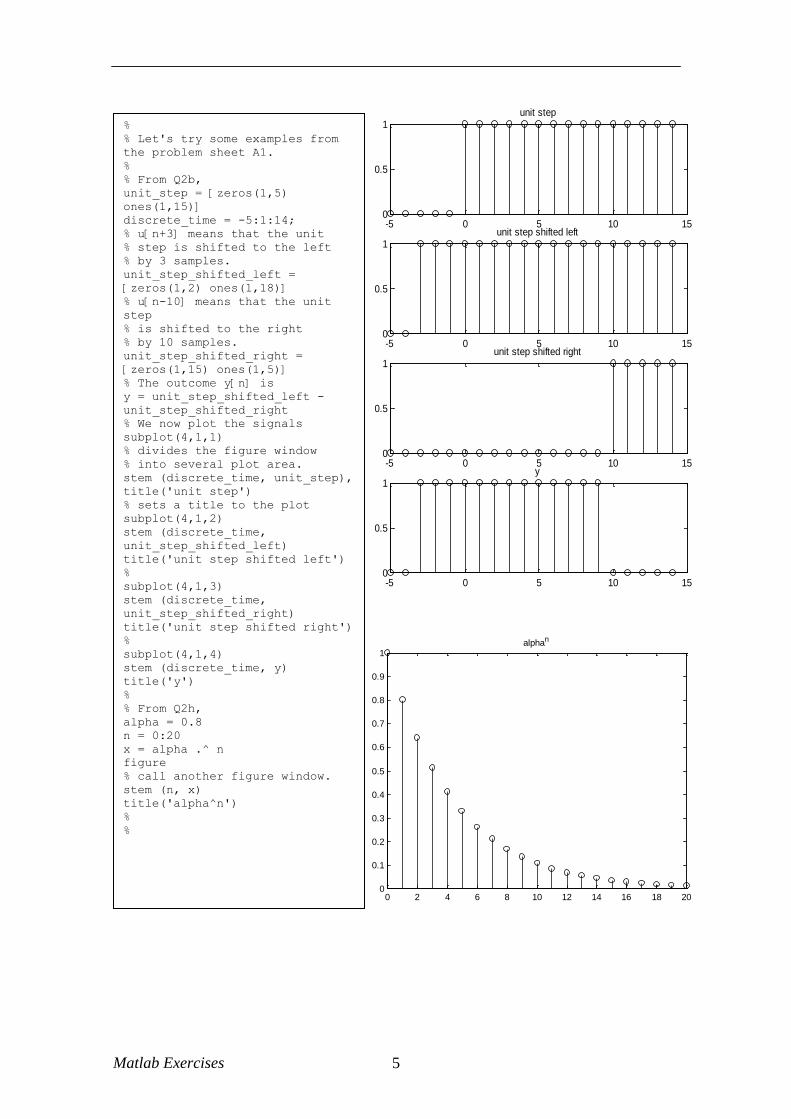
% Let's try some examples from

the problem sheet A1.

%

% From Q2b,

unit_step = [zeros(1,5)

ones(1,15)]

discrete_time = -5:1:14;

% u[n+3] means that the unit

% step is shifted to the left

% by 3 samples.

unit_step_shifted_left =

[zeros(1,2) ones(1,18)]

% u[n-10] means that the unit

step

% is shifted to the right

% by 10 samples.

unit_step_shifted_right =

[zeros(1,15) ones(1,5)]

% The outcome y[n] is

y = unit_step_shifted_left -

unit_step_shifted_right

% We now plot the signals

subplot(4,1,1)

% divides the figure window

% into several plot area.

stem (discrete_time, unit_step),

title('unit step')

% sets a title to the plot

subplot(4,1,2)

stem (discrete_time,

unit_step_shifted_left)

title('unit step shifted left')

%

subplot(4,1,3)

stem (discrete_time,

unit_step_shifted_right)

title('unit step shifted right')

%

subplot(4,1,4)

stem (discrete_time, y)

title('y')

%

% From Q2h,

alpha = 0.8

n = 0:20

x = alpha .^ n

figure

% call another figure window.

stem (n, x)

title('alpha^n')

%

%

Matlab Exercises 6

0 0.1 0.2 0.3 0.4 0.5 0.6 0.7 0.8 0.9 1-1

-0.8

-0.6

-0.4

-0.2

0

0.2

0.4

0.6

0.8

1continuous sinusoid

0 10 20 30 40 50 60 70 80 90 100-1

-0.5

0

0.5

1x=cos(n*pi/8)

0 10 20 30 40 50 60 70 80 90 100-1

-0.5

0

0.5

1y=cos(n*pi/16

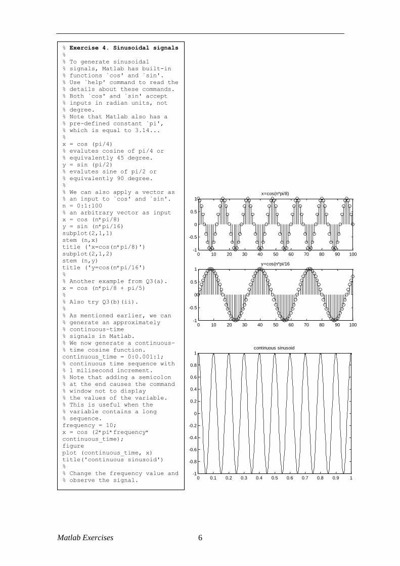
% Exercise 4. Sinusoidal signals

%

% To generate sinusoidal

% signals, Matlab has built-in

% functions `cos' and `sin'.

% Use `help' command to read the

% details about these commands.

% Both `cos' and `sin' accept

% inputs in radian units, not

% degree.

% Note that Matlab also has a

% pre-defined constant `pi',

% which is equal to 3.14...

%

x = cos (pi/4)

% evalutes cosine of pi/4 or

% equivalently 45 degree.

y = sin (pi/2)

% evalutes sine of pi/2 or

% equivalently 90 degree.

%

% We can also apply a vector as

% an input to `cos' and `sin'.

n = 0:1:100

% an arbitrary vector as input

x = cos (n*pi/8)

y = sin (n*pi/16)

subplot(2,1,1)

stem (n,x)

title ('x=cos(n*pi/8)')

subplot(2,1,2)

stem (n,y)

title ('y=cos(n*pi/16')

%

% Another example from Q3(a).

x = cos (n*pi/8 + pi/5)

%

% Also try Q3(b)(ii).

%

% As mentioned earlier, we can

% generate an approximately

% continuous-time

% signals in Matlab.

% We now generate a continuous-

% time cosine function.

continuous_time = 0:0.001:1;

% continuous time sequence with

% 1 milisecond increment.

% Note that adding a semicolon

% at the end causes the command

% window not to display

% the values of the variable.

% This is useful when the

% variable contains a long

% sequence.

frequency = 10;

x = cos (2*pi*frequency*

continuous_time);

figure

plot (continuous_time, x)

title('continuous sinusoid')

%

% Change the frequency value and

% observe the signal.

Matlab Exercises 7


-20 -15 -10 -5 0 5 10 15 200

0.5

1unit step

-20 -15 -10 -5 0 5 10 15 200

0.5

1unit step shifted left

-20 -15 -10 -5 0 5 10 15 200

0.5

1unit step shifted right

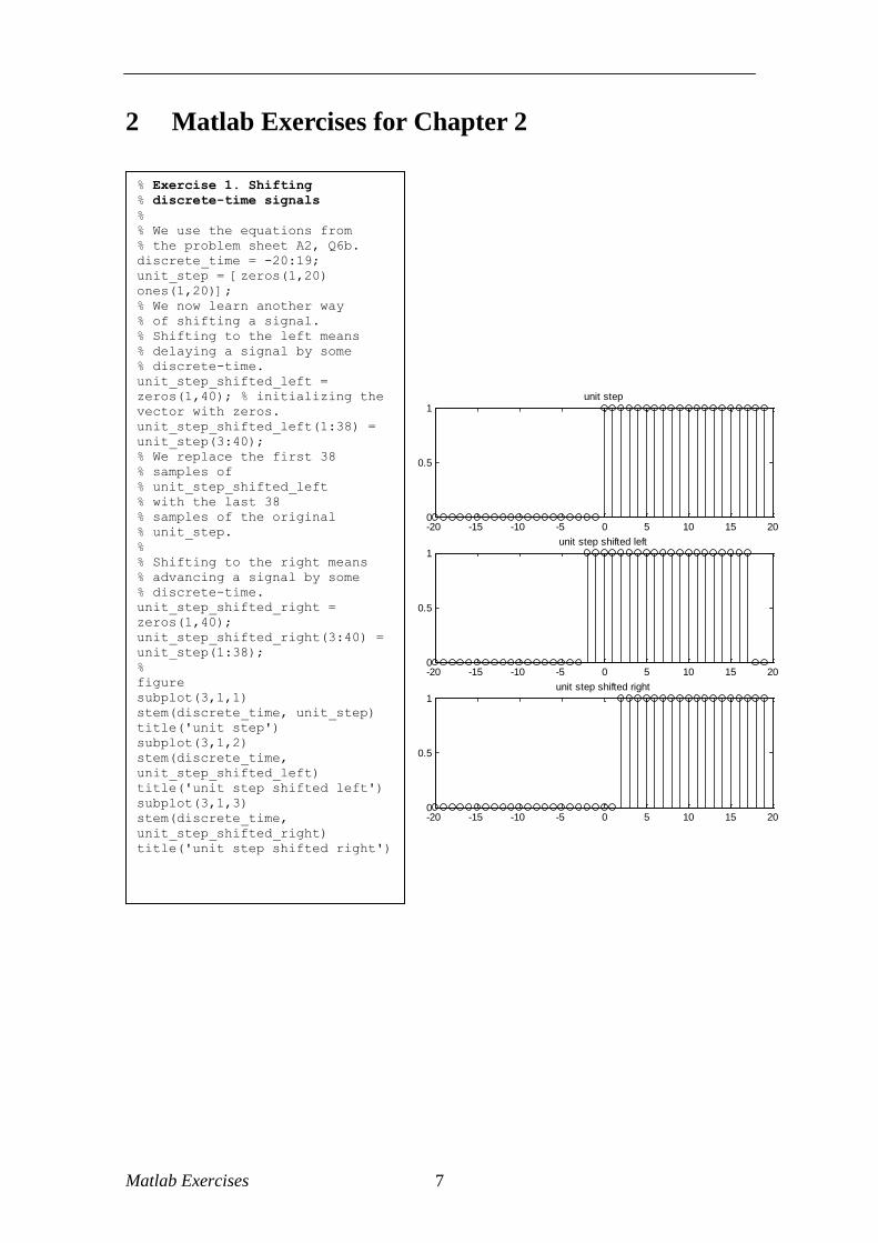
% Exercise 1. Shifting

% discrete-time signals

%

% We use the equations from

% the problem sheet A2, Q6b.

discrete_time = -20:19;

unit_step = [zeros(1,20)

ones(1,20)];

% We now learn another way

% of shifting a signal.

% Shifting to the left means

% delaying a signal by some

% discrete-time.

unit_step_shifted_left =

zeros(1,40); % initializing the

vector with zeros.

unit_step_shifted_left(1:38) =

unit_step(3:40);

% We replace the first 38

% samples of

% unit_step_shifted_left

% with the last 38

% samples of the original

% unit_step.

%

% Shifting to the right means

% advancing a signal by some

% discrete-time.

unit_step_shifted_right =

zeros(1,40);

unit_step_shifted_right(3:40) =

unit_step(1:38);

%

figure

subplot(3,1,1)

stem(discrete_time, unit_step)

title('unit step')

subplot(3,1,2)

stem(discrete_time,

unit_step_shifted_left)

title('unit step shifted left')

subplot(3,1,3)

stem(discrete_time,

unit_step_shifted_right)

title('unit step shifted right')

Matlab Exercises 8

0 2 4 6 8 10 12 14 16 18 200

0.005

0.01

0.015

0.02

0.025

0.03

0.035

0.04

0.045

0.05impulse response

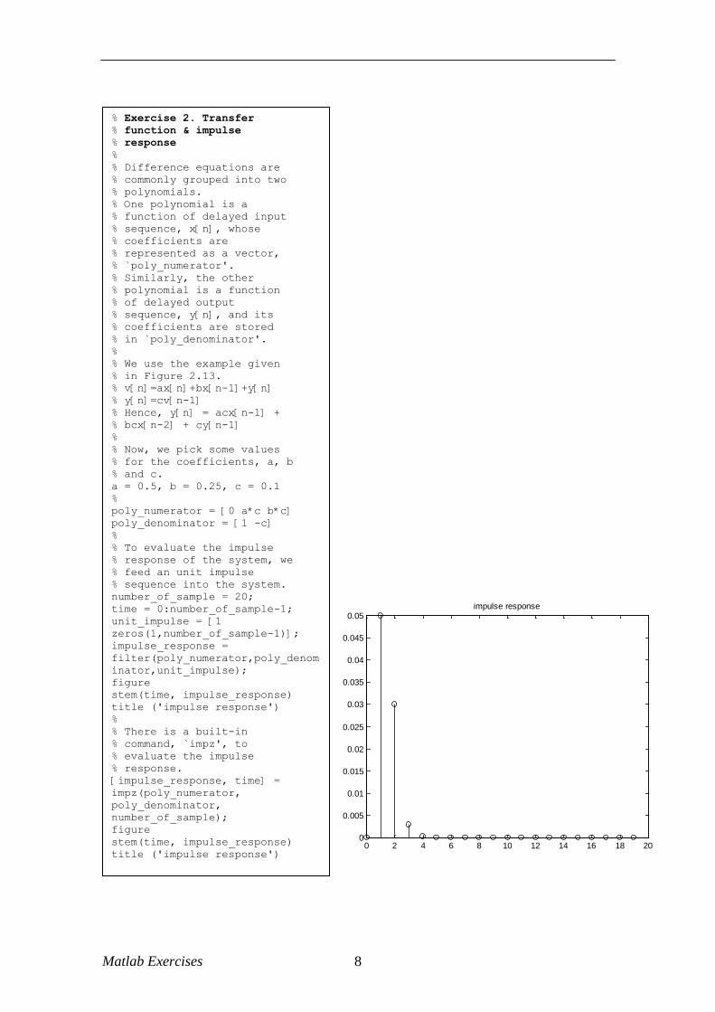
% Exercise 2. Transfer

% function & impulse

% response

%

% Difference equations are

% commonly grouped into two

% polynomials.

% One polynomial is a

% function of delayed input

% sequence, x[n], whose

% coefficients are

% represented as a vector,

% `poly_numerator'.

% Similarly, the other

% polynomial is a function

% of delayed output

% sequence, y[n], and its

% coefficients are stored

% in `poly_denominator'.

%

% We use the example given

% in Figure 2.13.

% v[n]=ax[n]+bx[n-1]+y[n]

% y[n]=cv[n-1]

% Hence, y[n] = acx[n-1] +

% bcx[n-2] + cy[n-1]

%

% Now, we pick some values

% for the coefficients, a, b

% and c.

a = 0.5, b = 0.25, c = 0.1

%

poly_numerator = [0 a*c b*c]

poly_denominator = [1 -c]

%

% To evaluate the impulse

% response of the system, we

% feed an unit impulse

% sequence into the system.

number_of_sample = 20;

time = 0:number_of_sample-1;

unit_impulse = [1

zeros(1,number_of_sample-1)];

impulse_response =

filter(poly_numerator,poly_denom

inator,unit_impulse);

figure

stem(time, impulse_response)

title ('impulse response')

%

% There is a built-in

% command, ìmpz', to

% evaluate the impulse

% response.

[impulse_response, time] =

impz(poly_numerator,

poly_denominator,

number_of_sample);

figure

stem(time, impulse_response)

title ('impulse response')

Matlab Exercises 9

-5 -4 -3 -2 -1 0 1 2 3 4 50

0.2

0.4

0.6

0.8

1x[n]

-5 -4 -3 -2 -1 0 1 2 3 4 50

1

2

3h[n]

-5 -4 -3 -2 -1 0 1 2 3 4 50

1

2

3y[n]

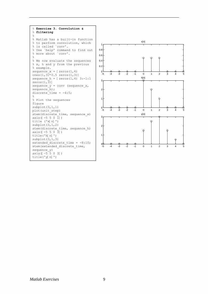
% Exercise 3. Convolution &

% filtering

%

% Matlab has a built-in function

% to perform convolution, which

% is called `conv'.

% Use `help' command to find out

% more about `conv'.

%

% We now evaluate the sequences

% x, h and y from the previous

% example.

sequence_x = [zeros(1,4)

ones(1,3)*0.5 zeros(1,3)]

sequence_h = [zeros(1,4) 3:-1:1

zeros(1,3)]

sequence_y = conv (sequence_x,

sequence_h);

discrete_time = -4:5;

%

% Plot the sequences

figure

subplot(3,1,1)

plot(unit_step)

stem(discrete_time, sequence_x)

axis([-5 5 0 1])

title ('x[n]')

subplot(3,1,2)

stem(discrete_time, sequence_h)

axis([-5 5 0 3])

title('h[n]')

subplot(3,1,3)

extended_discrete_time = -8:10;

stem(extended_discrete_time,

sequence_y)

axis([-5 5 0 3])

title('y[n]')

Matlab Exercises 10


0 0.1 0.2 0.3 0.4 0.5 0.6 0.7 0.8 0.9 1-5

0

5

10

Normalized Angular Frequency ( rads/sample)

Magnitude (

dB

)

0 0.1 0.2 0.3 0.4 0.5 0.6 0.7 0.8 0.9 1-30

-20

-10

0


Phase (

degre

es)

-1 -0.5 0 0.5 1

-1

-0.8

-0.6

-0.4

-0.2

0

0.2

0.4

0.6

0.8

1

Real Part

Imagin

ary

Part

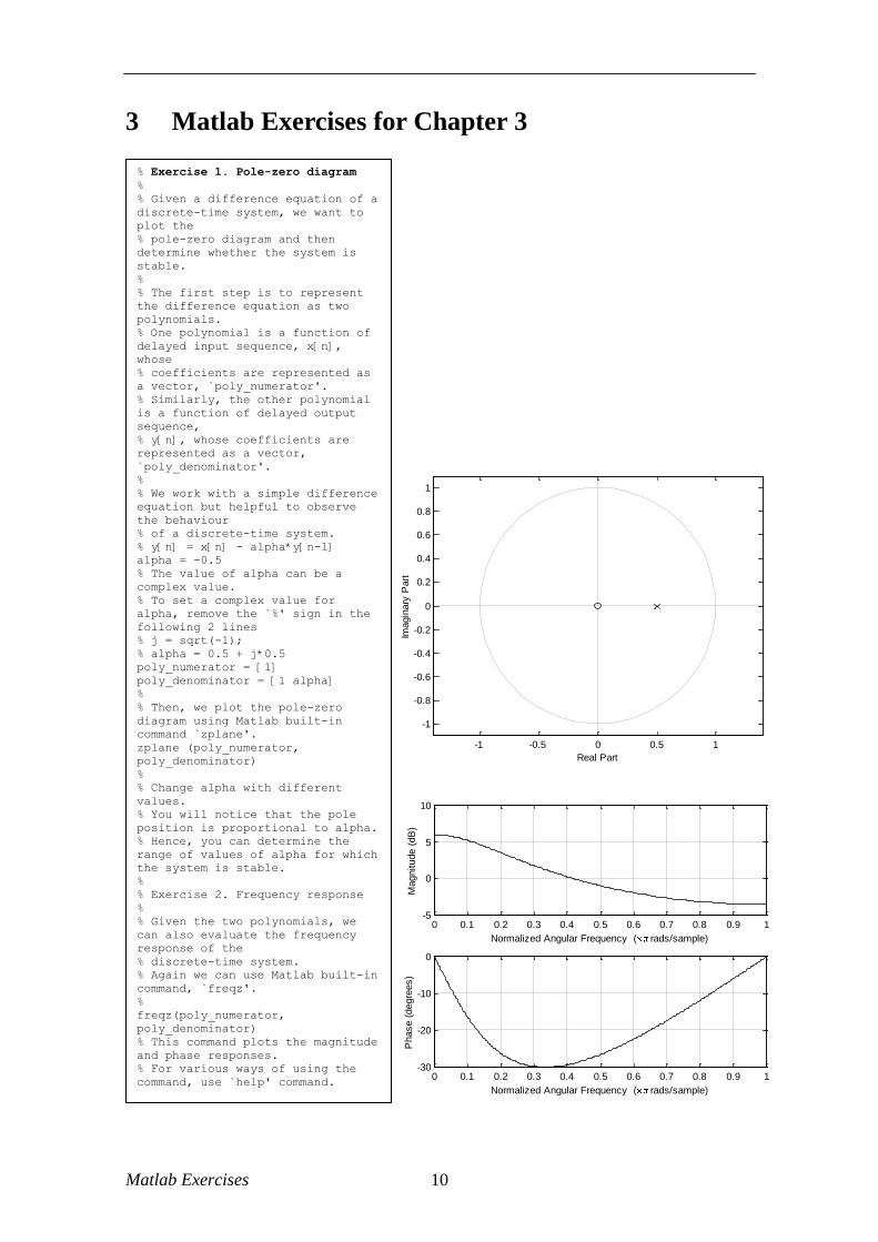
% Exercise 1. Pole-zero diagram

%

% Given a difference equation of a

discrete-time system, we want to

plot the

% pole-zero diagram and then

determine whether the system is

stable.

%

% The first step is to represent

the difference equation as two

polynomials.

% One polynomial is a function of

delayed input sequence, x[n],

whose

% coefficients are represented as

a vector, `poly_numerator'.

% Similarly, the other polynomial

is a function of delayed output

sequence,

% y[n], whose coefficients are

represented as a vector,

`poly_denominator'.

%

% We work with a simple difference

equation but helpful to observe

the behaviour

% of a discrete-time system.

% y[n] = x[n] - alpha*y[n-1]

alpha = -0.5

% The value of alpha can be a

complex value.

% To set a complex value for

alpha, remove the `%' sign in the

following 2 lines

% j = sqrt(-1);

% alpha = 0.5 + j*0.5

poly_numerator = [1]

poly_denominator = [1 alpha]

%

% Then, we plot the pole-zero

diagram using Matlab built-in

command `zplane'.

zplane (poly_numerator,

poly_denominator)

%

% Change alpha with different

values.

% You will notice that the pole

position is proportional to alpha.

% Hence, you can determine the

range of values of alpha for which

the system is stable.

%

% Exercise 2. Frequency response

%

% Given the two polynomials, we

can also evaluate the frequency

response of the

% discrete-time system.

% Again we can use Matlab built-in

command, `freqz'.

%

freqz(poly_numerator,

poly_denominator)

% This command plots the magnitude

and phase responses.

% For various ways of using the

command, use `help' command.

% Change alpha with different

values and observe the impact on

the magnitude response.

Matlab Exercises 11

0 500 1000 1500 2000 2500 3000 3500 4000-40

-20

0

20

40

Frequency (Hz)

Magnitude (

dB

)

0 500 1000 1500 2000 2500 3000 3500 4000-150

-100

-50

0

50

Frequency (Hz)

Phase (

degre

es)

-1 -0.5 0 0.5 1

-1

-0.8

-0.6

-0.4

-0.2

0

0.2

0.4

0.6

0.8

1

Real Part

Imagin

ary

Part

0 5 10 15 20 250

0.1

0.2

0.3

0.4

0.5

0.6

0.7

0.8

0.9

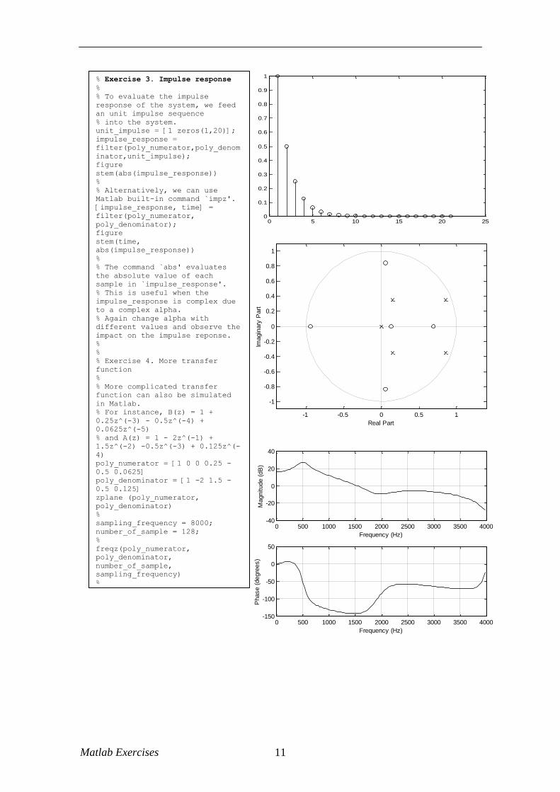
1% Exercise 3. Impulse response

%

% To evaluate the impulse

response of the system, we feed

an unit impulse sequence

% into the system.

unit_impulse = [1 zeros(1,20)];

impulse_response =

filter(poly_numerator,poly_denom

inator,unit_impulse);

figure

stem(abs(impulse_response))

%

% Alternatively, we can use

Matlab built-in command ìmpz'.

[impulse_response, time] =

filter(poly_numerator,

poly_denominator);

figure

stem(time,

abs(impulse_response))

%

% The command àbs' evaluates

the absolute value of each

sample in ìmpulse_response'.

% This is useful when the

impulse_response is complex due

to a complex alpha.

% Again change alpha with

different values and observe the

impact on the impulse reponse.

%

%

% Exercise 4. More transfer

function

%

% More complicated transfer

function can also be simulated

in Matlab.

% For instance, B(z) = 1 +

0.25z^(-3) - 0.5z^(-4) +

0.0625z^(-5)

% and A(z) = 1 - 2z^(-1) +

1.5z^(-2) -0.5z^(-3) + 0.125z^(-

4)

poly_numerator = [1 0 0 0.25 -

0.5 0.0625]

poly_denominator = [1 -2 1.5 -

0.5 0.125]

zplane (poly_numerator,

poly_denominator)

%

sampling_frequency = 8000;

number_of_sample = 128;

%

freqz(poly_numerator,

poly_denominator,

number_of_sample,

sampling_frequency)

%

Matlab Exercises 12

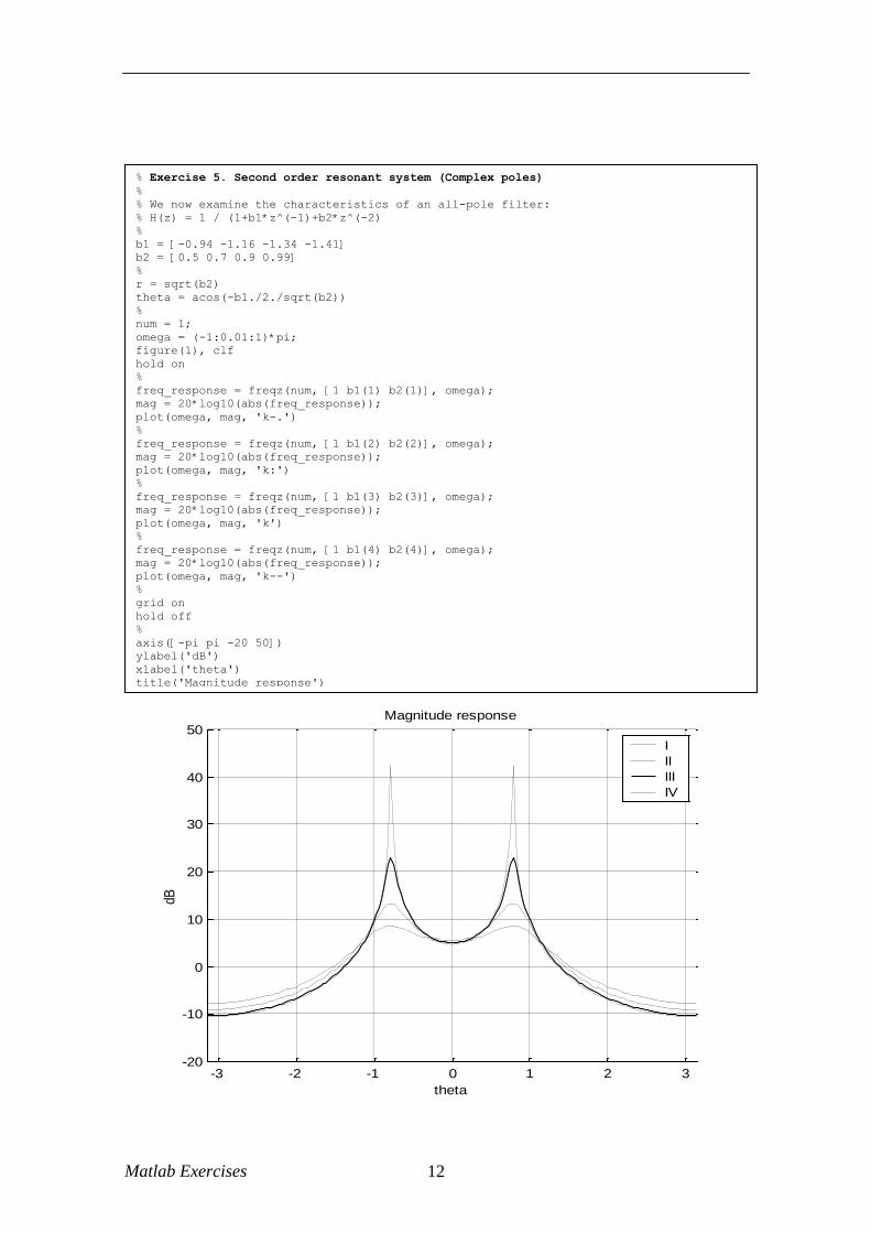
% Exercise 5. Second order resonant system (Complex poles)

%

% We now examine the characteristics of an all-pole filter:

% H(z) = 1 / (1+b1*z^(-1)+b2*z^(-2)

%

b1 = [-0.94 -1.16 -1.34 -1.41]

b2 = [0.5 0.7 0.9 0.99]

%

r = sqrt(b2)

theta = acos(-b1./2./sqrt(b2))

%

num = 1;

omega = (-1:0.01:1)*pi;

figure(1), clf

hold on

%

freq_response = freqz(num, [1 b1(1) b2(1)], omega);

mag = 20*log10(abs(freq_response));

plot(omega, mag, 'k-.')

%



plot(omega, mag, 'k:')

%



plot(omega, mag, 'k')

%



plot(omega, mag, 'k--')

%

grid on

hold off

%

axis([-pi pi -20 50])

ylabel('dB')

xlabel('theta')

title('Magnitude response')

-3 -2 -1 0 1 2 3-20

-10

0

10

20

30

40

50

dB

theta

Magnitude response

I

II

III

IV

Matlab Exercises 13


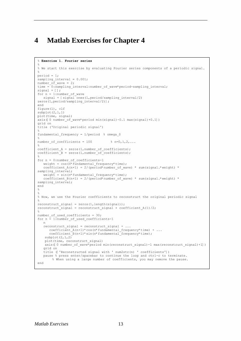
% Exercise 1. Fourier series

%

% We start this exercise by evaluating Fourier series components of a periodic signal.

%

period = 1;

sampling_interval = 0.001;

number_of_wave = 2;

time = 0:sampling_interval:number_of_wave*period-sampling_interval;

signal = [];

for n = 1:number_of_wave

signal = [signal ones(1,period/sampling_interval/2)

zeros(1,period/sampling_interval/2)];

end

figure(1), clf

subplot(2,1,1)

plot(time, signal)

axis([0 number_of_wave*period min(signal)-0.1 max(signal)+0.1])

grid on

title ('Original periodic signal')

%

fundamental_frequency = 1/period % omega_0

%

number_of_coefficients = 100 % n=0,1,2,...

%

coefficient_A = zeros(1,number_of_coefficients);

coefficient_B = zeros(1,number_of_coefficients);

%

for n = 0:number_of_coefficients-1

weight = cos(n*fundamental_frequency*time);

coefficient_A(n+1) = 2/(period*number_of_wave) * sum(signal.*weight) *

sampling_interval;

weight = sin(n*fundamental_frequency*time);

coefficient_B(n+1) = 2/(period*number_of_wave) * sum(signal.*weight) *

sampling_interval;

end

%

%

% Now, we use the Fourier coefficients to reconstruct the original periodic signal

%

reconstruct_signal = zeros(1,length(signal));

reconstruct_signal = reconstruct_signal + coefficient_A(1)/2;

%

number_of_used_coefficients = 30;

for n = 1:number_of_used_coefficients-1

n

reconstruct_signal = reconstruct_signal + ...

coefficient_A(n+1)*cos(n*fundamental_frequency*time) + ...

coefficient_B(n+1)*sin(n*fundamental_frequency*time);

subplot(2,1,2)

plot(time, reconstruct_signal)

axis([0 number_of_wave*period min(reconstruct_signal)-1 max(reconstruct_signal)+1])

grid on

title (['Reconstructed signal with ' num2str(n) ' coefficients'])

pause % press enter/spacebar to continue the loop and ctrl-c to terminate.

% When using a large number of coefficients, you may remove the pause.

end

Matlab Exercises 14

0 0.5 1 1.5 2

0

0.2

0.4

0.6

0.8

1

Original periodic signal

0 0.5 1 1.5 2 -0.5

0

0.5

1

1.5 Reconstructed signal with 1 coefficient

0 0.5 1 1.5 2

-2

-1

0

1

2

3

Reconstructed signal with 10 coefficients

-2

-1

0 0.5 1 1.5 2

0

1

2

3


0 0.5 1 1.5 2 -2

-1

0

1

2

3


0 0.5 1 1.5 2 -2

-1

0

1

2

3


Matlab Exercises 15


0 0.1 0.2 0.3 0.4 0.5 0.6 0.7 0.8 0.9 10

5

10

15

20


Magnitude (

dB

)

0 0.1 0.2 0.3 0.4 0.5 0.6 0.7 0.8 0.9 1-800

-600

-400

-200

0


Phase (

degre

es)

-2.5 -2 -1.5 -1 -0.5 0 0.5 1 1.5

-1.5

-1

-0.5

0

0.5

1

1.5

Real Part

Imagin

ary

Part

3

%

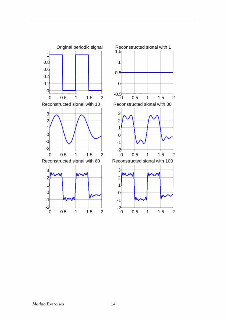
% Exercise 1. Minimum and

maximum phase filter

%

% We examine the properties of

minimum and maximum phase

filter

%

% We start with a maximum

phase filter from the example

in page 64.

%

zeros_maxphase = [3/2 -4/3 -

5/2]' % zeros position

% Note the transpose operation

since the inputs are zeros and

poles.

% If the inputs are row

vectors, they will be treated

as polynomial coefficents.

poles_maxphase = [0 0 0]' % poles are located at origin

%

% After specifying the poles

and zeros position, we now

plot their position.

figure(1) % create a new

figure (No.1)

zplane(zeros_maxphase,

poles_maxphase)

%

% We also find the numerator

and denominator coefficients

of the transfer function

% in order to plot the

magnitude and phase responses.

numerator_maxphase =

poly(zeros_maxphase)

denominator_maxphase = 1; %

since all poles are at origin


figure (No.2)

freqz(numerator_maxphase,

denominator_maxphase)

%

Matlab Exercises 16

%

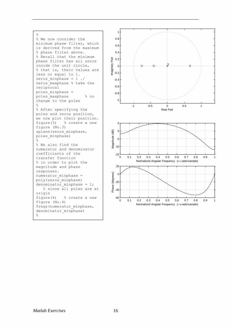
% We now consider the

minimum phase filter, which

is derived from the maximum

% phase filter above.

% Recall that the minimum

phase filter has all zeros

inside the unit circle,

% that is, their values are

less or equal to 1.

zeros_minphase = 1 ./

zeros_maxphase % take the

reciprocal

poles_minphase =

poles_maxphase % no

change to the poles

%

% After specifying the

poles and zeros position,

we now plot their position.


figure (No.3)

zplane(zeros_minphase,

poles_minphase)

%

% We also find the

numerator and denominator

coefficients of the

transfer function

% in order to plot the

magnitude and phase

responses.

numerator_minphase =

poly(zeros_minphase)

denominator_minphase = 1;

% since all poles are at

origin


figure (No.4)

freqz(numerator_minphase,

denominator_minphase)

%

0 0.1 0.2 0.3 0.4 0.5 0.6 0.7 0.8 0.9 1-15

-10

-5

0

5


Magnitude (

dB

)

0 0.1 0.2 0.3 0.4 0.5 0.6 0.7 0.8 0.9 1-60

-40

-20

0

20


Phase (

degre

es)

-1 -0.5 0 0.5 1

-1

-0.8

-0.6

-0.4

-0.2

0

0.2

0.4

0.6

0.8

1

Real PartIm

agin

ary

Part

3

Matlab Exercises 17

0 10 20 30 40 50 60 70 80 90 100-2.5

-2

-1.5

-1

-0.5

0

0.5

1

1.5

2

2.5

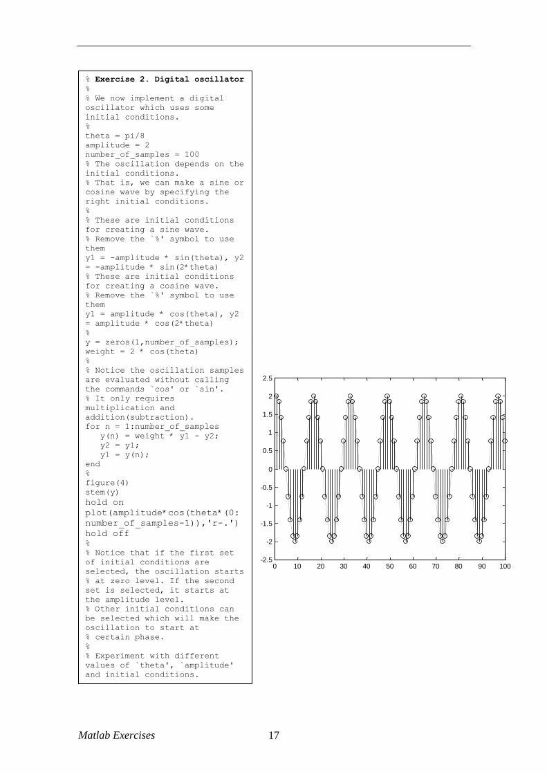
% Exercise 2. Digital oscillator

%

% We now implement a digital

oscillator which uses some

initial conditions.

%

theta = pi/8 % angular frequency of the oscillator

amplitude = 2 % amplitude of the oscillator

number_of_samples = 100

% The oscillation depends on the

initial conditions.

% That is, we can make a sine or

cosine wave by specifying the

right initial conditions.

%

% These are initial conditions

for creating a sine wave.

% Remove the `%' symbol to use

them

y1 = -amplitude * sin(theta), y2

= -amplitude * sin(2*theta)

% These are initial conditions

for creating a cosine wave.

% Remove the `%' symbol to use

them

y1 = amplitude * cos(theta), y2

= amplitude * cos(2*theta)

%

y = zeros(1,number_of_samples); % initializing oscillation samples

weight = 2 * cos(theta)

%

% Notice the oscillation samples

are evaluated without calling

the commands `cos' or `sin'.

% It only requires

multiplication and

addition(subtraction).

for n = 1:number_of_samples

y(n) = weight * y1 - y2;

y2 = y1; % updating previous samples

y1 = y(n);

end

%

figure(4)

stem(y)

hold on

plot(amplitude*cos(theta*(0:

number_of_samples-1)),'r-.')

hold off

%

% Notice that if the first set

of initial conditions are

selected, the oscillation starts

% at zero level. If the second

set is selected, it starts at

the amplitude level.

% Other initial conditions can

be selected which will make the

oscillation to start at

% certain phase.

%

% Experiment with different

values of `theta', àmplitude'

and initial conditions.

%

Matlab Exercises 18


0 10 20 30 40 50 60 70 80 90 100-1

-0.5

0

0.5

1

-1 -0.8 -0.6 -0.4 -0.2 0 0.2 0.4 0.6 0.8 10

10

20

30

40

50

60

Normalized frequency, 1 corresponds to pi

Magnitude

Discrete-time Fourier Transform

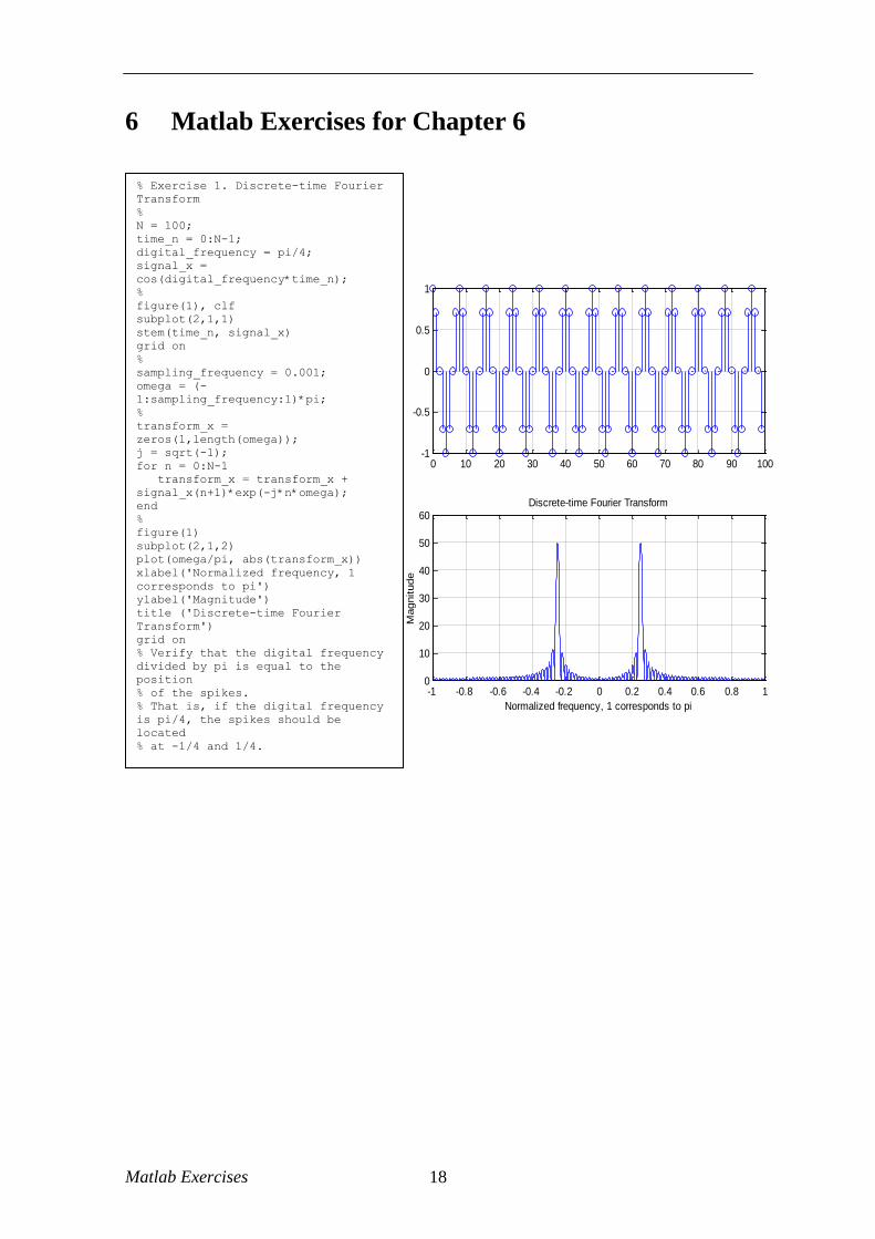
% Exercise 1. Discrete-time Fourier

Transform

%

N = 100;

time_n = 0:N-1;

digital_frequency = pi/4;

signal_x =

cos(digital_frequency*time_n);

%

figure(1), clf

subplot(2,1,1)

stem(time_n, signal_x)

grid on

%

sampling_frequency = 0.001;

omega = (-

1:sampling_frequency:1)*pi;

%

transform_x =

zeros(1,length(omega));

j = sqrt(-1);

for n = 0:N-1

transform_x = transform_x +

signal_x(n+1)*exp(-j*n*omega);

end

%

figure(1)

subplot(2,1,2)

plot(omega/pi, abs(transform_x))

xlabel('Normalized frequency, 1

corresponds to pi')

ylabel('Magnitude')

title ('Discrete-time Fourier

Transform')

grid on

% Verify that the digital frequency

divided by pi is equal to the

position

% of the spikes.

% That is, if the digital frequency

is pi/4, the spikes should be

located

% at -1/4 and 1/4.

Matlab Exercises 19

0 10 20 30 40 50 60 70 80 90 100-1

-0.5

0

0.5

1signal x

0 10 20 30 40 50 60 70 80 90 1000

10

20

30

40Fourier Transform of x

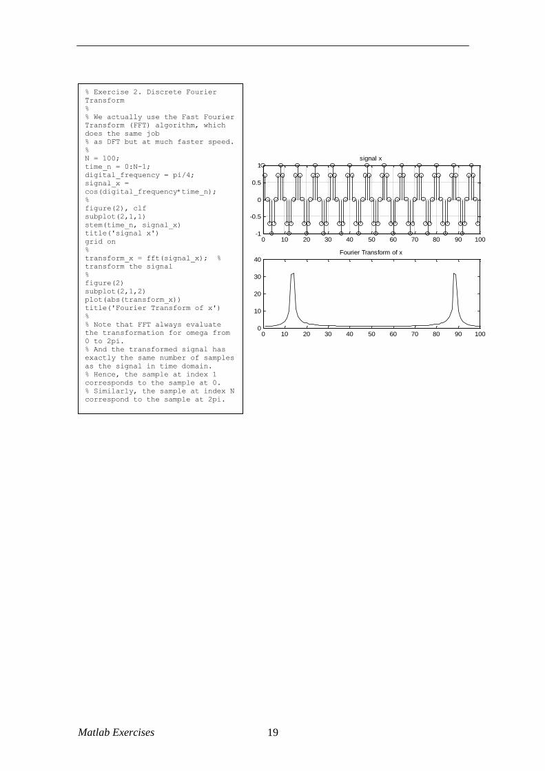
% Exercise 2. Discrete Fourier

Transform

%

% We actually use the Fast Fourier

Transform (FFT) algorithm, which

does the same job

% as DFT but at much faster speed.

%

N = 100;

time_n = 0:N-1;


signal_x =

cos(digital_frequency*time_n);

%

figure(2), clf

subplot(2,1,1)


title('signal x')

grid on

%

transform_x = fft(signal_x); %

transform the signal

%

figure(2)

subplot(2,1,2)

plot(abs(transform_x))

title('Fourier Transform of x')

%

% Note that FFT always evaluate

the transformation for omega from

0 to 2pi.

% And the transformed signal has

exactly the same number of samples

as the signal in time domain.

% Hence, the sample at index 1

corresponds to the sample at 0.

% Similarly, the sample at index N

correspond to the sample at 2pi.

Matlab Exercises 20

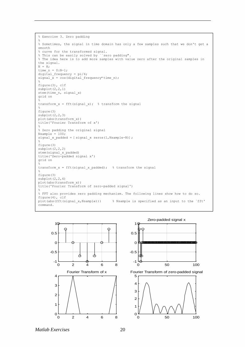
% Exercise 3. Zero padding

%

% Sometimes, the signal in time domain has only a few samples such that we don't get a

smooth

% curve for the transformed signal.

% This can be easily solved by ``zero padding".

% The idea here is to add more samples with value zero after the original samples in

the signal.

N = 8;

time_n = 0:N-1;


signal_x = cos(digital_frequency*time_n);

%

figure(3), clf

subplot(2,2,1)


grid on

%

transform_x = fft(signal_x); % transform the signal

%

figure(3)

subplot(2,2,3)


title('Fourier Transform of x')

%

% Zero padding the original signal

Nsample = 100;

signal_x_padded = [signal_x zeros(1,Nsample-N)];

%

figure(3)

subplot(2,2,2)

stem(signal_x_padded)

title('Zero-padded signal x')

grid on

%

transform_x = fft(signal_x_padded); % transform the signal

%

figure(3)

subplot(2,2,4)


title('Fourier Transform of zero-padded signal')

%

% FFT also provides zero padding mechanism. The following lines show how to do so.

figure(4), clf

plot(abs(fft(signal_x,Nsample))) % Nsample is specified as an input to the `fft'

command.

0 2 4 6 8-1

-0.5

0

0.5

1

0 2 4 6 80

1

2

3

4Fourier Transform of x

0 50 100-1

-0.5

0

0.5

1Zero-padded signal x

0 50 1000

1

2

3

4

5Fourier Transform of zero-padded signal

Matlab Exercises 21


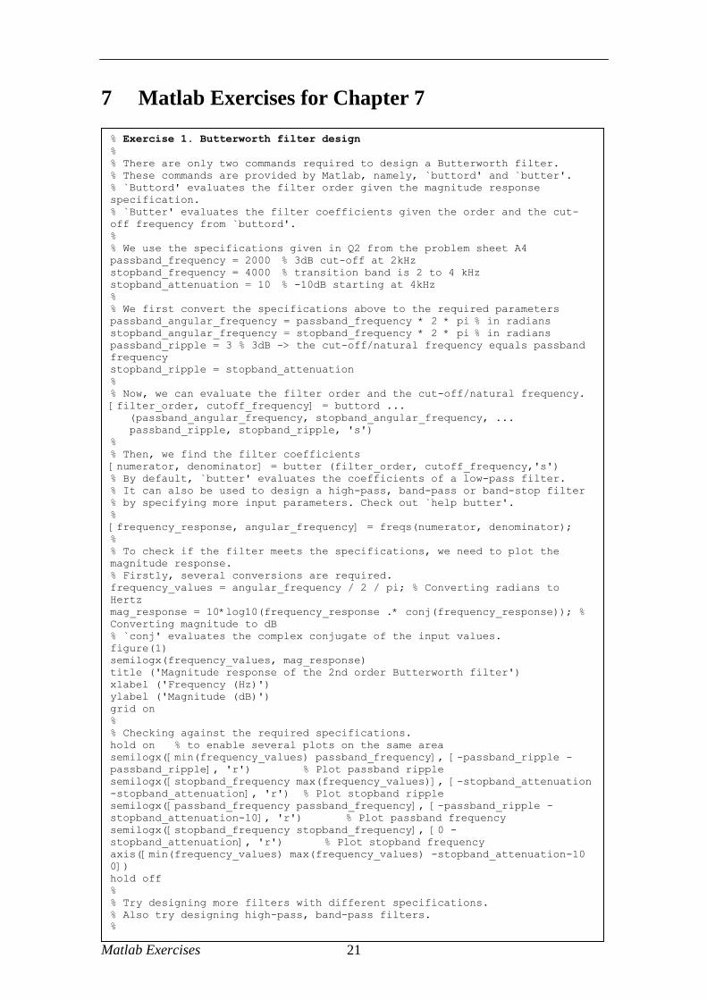
% Exercise 1. Butterworth filter design

%

% There are only two commands required to design a Butterworth filter.

% These commands are provided by Matlab, namely, `buttord' and `butter'.

% `Buttord' evaluates the filter order given the magnitude response

specification.

% `Butter' evaluates the filter coefficients given the order and the cut-

off frequency from `buttord'.

%

% We use the specifications given in Q2 from the problem sheet A4

passband_frequency = 2000 % 3dB cut-off at 2kHz

stopband_frequency = 4000 % transition band is 2 to 4 kHz

stopband_attenuation = 10 % -10dB starting at 4kHz

%

% We first convert the specifications above to the required parameters

passband_angular_frequency = passband_frequency * 2 * pi % in radians

stopband_angular_frequency = stopband_frequency * 2 * pi % in radians

passband_ripple = 3 % 3dB -> the cut-off/natural frequency equals passband

frequency

stopband_ripple = stopband_attenuation

%

% Now, we can evaluate the filter order and the cut-off/natural frequency.

[filter_order, cutoff_frequency] = buttord ...

(passband_angular_frequency, stopband_angular_frequency, ...

passband_ripple, stopband_ripple, 's')

%

% Then, we find the filter coefficients

[numerator, denominator] = butter (filter_order, cutoff_frequency,'s')

% By default, `butter' evaluates the coefficients of a low-pass filter.

% It can also be used to design a high-pass, band-pass or band-stop filter

% by specifying more input parameters. Check out `help butter'.

%

[frequency_response, angular_frequency] = freqs(numerator, denominator);

%

% To check if the filter meets the specifications, we need to plot the

magnitude response.

% Firstly, several conversions are required.

frequency_values = angular_frequency / 2 / pi; % Converting radians to

Hertz

mag_response = 10*log10(frequency_response .* conj(frequency_response)); %

Converting magnitude to dB

% `conj' evaluates the complex conjugate of the input values.

figure(1)

semilogx(frequency_values, mag_response)

title ('Magnitude response of the 2nd order Butterworth filter')

xlabel ('Frequency (Hz)')

ylabel ('Magnitude (dB)')

grid on

%

% Checking against the required specifications.

hold on % to enable several plots on the same area

semilogx([min(frequency_values) passband_frequency], [-passband_ripple -

passband_ripple], 'r') % Plot passband ripple

semilogx([stopband_frequency max(frequency_values)], [-stopband_attenuation

-stopband_attenuation], 'r') % Plot stopband ripple

semilogx([passband_frequency passband_frequency], [-passband_ripple -

stopband_attenuation-10], 'r') % Plot passband frequency

semilogx([stopband_frequency stopband_frequency], [0 -

stopband_attenuation], 'r') % Plot stopband frequency

axis([min(frequency_values) max(frequency_values) -stopband_attenuation-10

0])

hold off

%

% Try designing more filters with different specifications.

% Also try designing high-pass, band-pass filters.

%

Matlab Exercises 22

103

104

-20

-18

-16

-14

-12

-10

-8

-6

-4

-2

0Magnitude response of the 2nd order Butterworth filter

Frequency (Hz)

Magnitude (

dB

)

Matlab Exercises 23

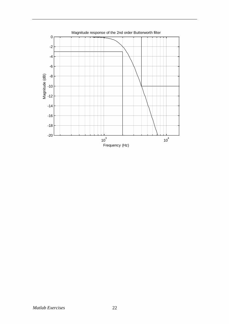
% Exercise 2. Chebyshev filter design

%

% The design process of a Chebyshev filter in Matlab is identical to that

of the

% Butterworth filter.

% Designing a Chebyshev type I filter only requires two commands, namely,

`Cheb1ord' and `Cheby1'.

% `Cheb1ord' evaluates the filter order given the magnitude response

specification.

% `Cheby1' evaluates the filter coefficients given the order and the cut-

off frequency from `Cheb1ord'.

%

% Chebyshev type II filter can be designed in the same way by using

commands

% `Cheb2ord' and `Cheby2'.

%

% We use the specifications given in Q4 from the problem sheet A4

passband_angular_frequency = 1000*pi % cut-off frequency at 1000pi rad/s

stopband_angular_frequency = 2000*pi % stopband frequency at 2000pi rad/s

passband_ripple = 1 % 1dB passband ripple

stopband_attenuation = 40 % 40dB stopband attenuation

%

% Now, we can evaluate the filter order and the cut-off/natural frequency.

[filter_order, cutoff_frequency] = cheb1ord ...

(passband_angular_frequency, stopband_angular_frequency, ...

passband_ripple, stopband_attenuation, 's')

%

% Then, we find the filter coefficients

[numerator, denominator] = cheby1 (filter_order, passband_ripple,

cutoff_frequency,'s')

[frequency_response, angular_frequency] = freqs(numerator, denominator);

%

% To check if the filter meets the specifications, we need to plot the

magnitude response.

% Firstly, several conversions are required.

frequency_values = angular_frequency / 2 / pi; % Converting radians to

Hertz

mag_response = 10*log10(frequency_response .* conj(frequency_response)); %

Converting magnitude to dB

% `conj' evaluates the complex conjugate of the input values.

figure(2)

semilogx(frequency_values, mag_response)

title ('Magnitude response of the Chebyshev filter')

xlabel ('Frequency (Hz)')

ylabel ('Magnitude (dB)')

grid on

%

% Checking against the required specifications.

hold on % to enable several plots on the same area

passband_frequency = passband_angular_frequency / 2 / pi

stopband_frequency = stopband_angular_frequency / 2 / pi

semilogx([min(frequency_values) passband_frequency], [-passband_ripple -

passband_ripple], 'r') % Plot passband ripple

semilogx([stopband_frequency max(frequency_values)], [-stopband_attenuation

-stopband_attenuation], 'r') % Plot stopband ripple

semilogx([passband_frequency passband_frequency], [-passband_ripple -

stopband_attenuation-10], 'r') % Plot passband frequency

semilogx([stopband_frequency stopband_frequency], [0 -

stopband_attenuation], 'r') % Plot stopband frequency

axis([min(frequency_values) max(frequency_values) -stopband_attenuation-10

0])

hold off

%

% Try designing more filters with different specifications.

% Also try designing high-pass, band-pass filters.

Matlab Exercises 24

101

102

103

-50

-45

-40

-35

-30

-25

-20

-15

-10

-5

0Magnitude response of the Chebyshev filter

Frequency (Hz)

Magnitude (

dB

)

Matlab Exercises 25


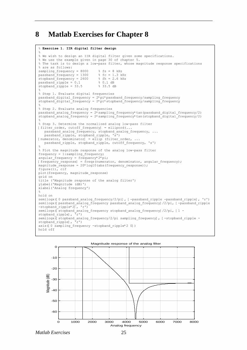
% Exercise 1. IIR digital filter design

%

% We wish to design an IIR digital filter given some specifications.

% We use the example given in page 30 of chapter 5.

% The task is to design a low-pass filter, whose magnitude response specifications

% are as follows:

sampling_frequency = 8000 % fs = 8 kHz

passband_frequency = 1300 % fc = 1.3 kHz

stopband_frequency = 2600 % fh = 2.6 kHz

passband_ripple = 0.1 % 0.1 dB

stopband_ripple = 33.5 % 33.5 dB

%

% Step 1. Evaluate digital frequencies

passband_digital_frequency = 2*pi*passband_frequency/sampling_frequency

stopband_digital_frequency = 2*pi*stopband_frequency/sampling_frequency

%

% Step 2. Evaluate analog frequencies

passband_analog_frequency = 2*sampling_frequency*tan(passband_digital_frequency/2)

stopband_analog_frequency = 2*sampling_frequency*tan(stopband_digital_frequency/2)

%

% Step 3. Determine the normalized analog low-pass filter

[filter_order, cutoff_frequency] = ellipord(...

passband_analog_frequency, stopband_analog_frequency, ...

passband_ripple, stopband_ripple, 's')

[numerator, denominator] = ellip (filter_order, ...

passband_ripple, stopband_ripple, cutoff_frequency, 's')

%

% Plot the magnitude response of the analog low-pass filter

frequency = 1:sampling_frequency;

angular_frequency = frequency*2*pi;

[frequency_response] = freqs(numerator, denominator, angular_frequency);

magnitude_response = 20*log10(abs(frequency_response));

figure(1), clf

plot(frequency, magnitude_response)

grid on

title ('Magnitude response of the analog filter')

ylabel('Magnitude (dB)')

xlabel('Analog frequency')

%

hold on

semilogx([0 passband_analog_frequency/2/pi], [-passband_ripple -passband_ripple], 'r')

semilogx([passband_analog_frequency passband_analog_frequency]/2/pi, [-passband_ripple

-stopband_ripple*2], 'r')

semilogx([stopband_analog_frequency stopband_analog_frequency]/2/pi, [1 -

stopband_ripple], 'r')

semilogx([stopband_analog_frequency/2/pi sampling_frequency], [-stopband_ripple -

stopband_ripple], 'r')

axis([0 sampling_frequency -stopband_ripple*2 0])

hold off

0 1000 2000 3000 4000 5000 6000 7000 8000

-60

-50

-40

-30

-20

-10

0Magnitude response of the analog filter

Mag

nitu

de (d

B)

Analog frequency

Matlab Exercises 26

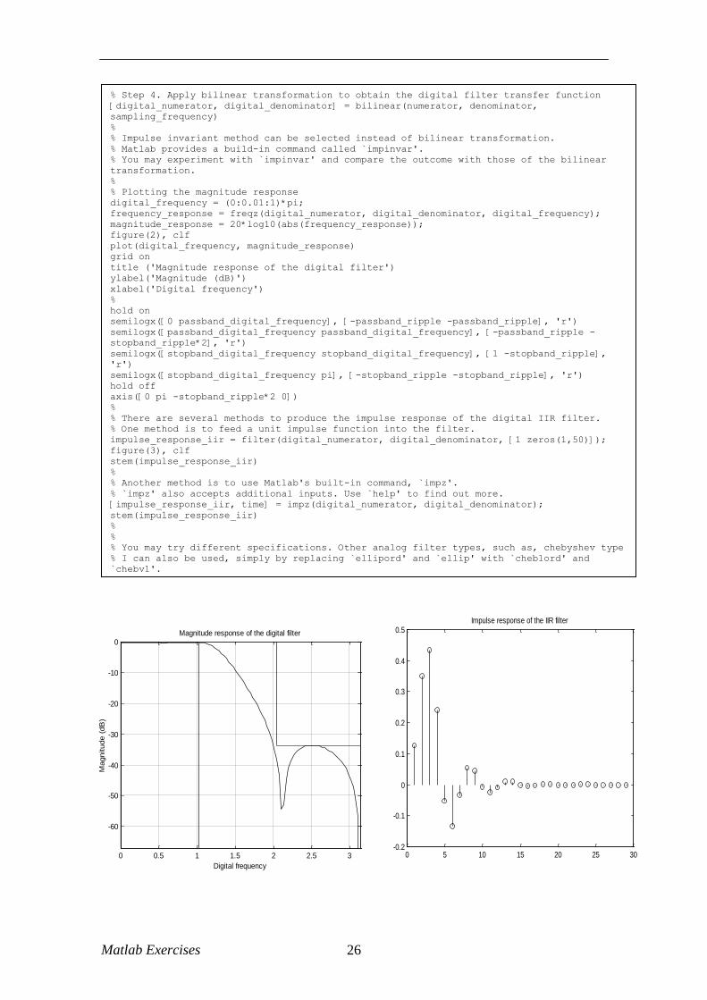
% Step 4. Apply bilinear transformation to obtain the digital filter transfer function

[digital_numerator, digital_denominator] = bilinear(numerator, denominator,

sampling_frequency)

%

% Impulse invariant method can be selected instead of bilinear transformation.

% Matlab provides a build-in command called ìmpinvar'.

% You may experiment with ìmpinvar' and compare the outcome with those of the bilinear

transformation.

%

% Plotting the magnitude response

digital_frequency = (0:0.01:1)*pi;

frequency_response = freqz(digital_numerator, digital_denominator, digital_frequency);


figure(2), clf

plot(digital_frequency, magnitude_response)

grid on

title ('Magnitude response of the digital filter')


xlabel('Digital frequency')

%

hold on

semilogx([0 passband_digital_frequency], [-passband_ripple -passband_ripple], 'r')

semilogx([passband_digital_frequency passband_digital_frequency], [-passband_ripple -

stopband_ripple*2], 'r')

semilogx([stopband_digital_frequency stopband_digital_frequency], [1 -stopband_ripple],

'r')

semilogx([stopband_digital_frequency pi], [-stopband_ripple -stopband_ripple], 'r')

hold off

axis([0 pi -stopband_ripple*2 0])

%

% There are several methods to produce the impulse response of the digital IIR filter.

% One method is to feed a unit impulse function into the filter.

impulse_response_iir = filter(digital_numerator, digital_denominator, [1 zeros(1,50)]);

figure(3), clf

stem(impulse_response_iir)

%

% Another method is to use Matlab's built-in command, ìmpz'.

% ìmpz' also accepts additional inputs. Use `help' to find out more.

[impulse_response_iir, time] = impz(digital_numerator, digital_denominator);

stem(impulse_response_iir)

%

%

% You may try different specifications. Other analog filter types, such as, chebyshev type

% I can also be used, simply by replacing èllipord' and èllip' with `cheb1ord' and

`cheby1'.

0 0.5 1 1.5 2 2.5 3

-60

-50

-40

-30

-20

-10

0Magnitude response of the digital filter

Magnitude (

dB

)

Digital frequency

0 5 10 15 20 25 30-0.2

-0.1

0

0.1

0.2

0.3

0.4

0.5Impulse response of the IIR filter

Matlab Exercises 27

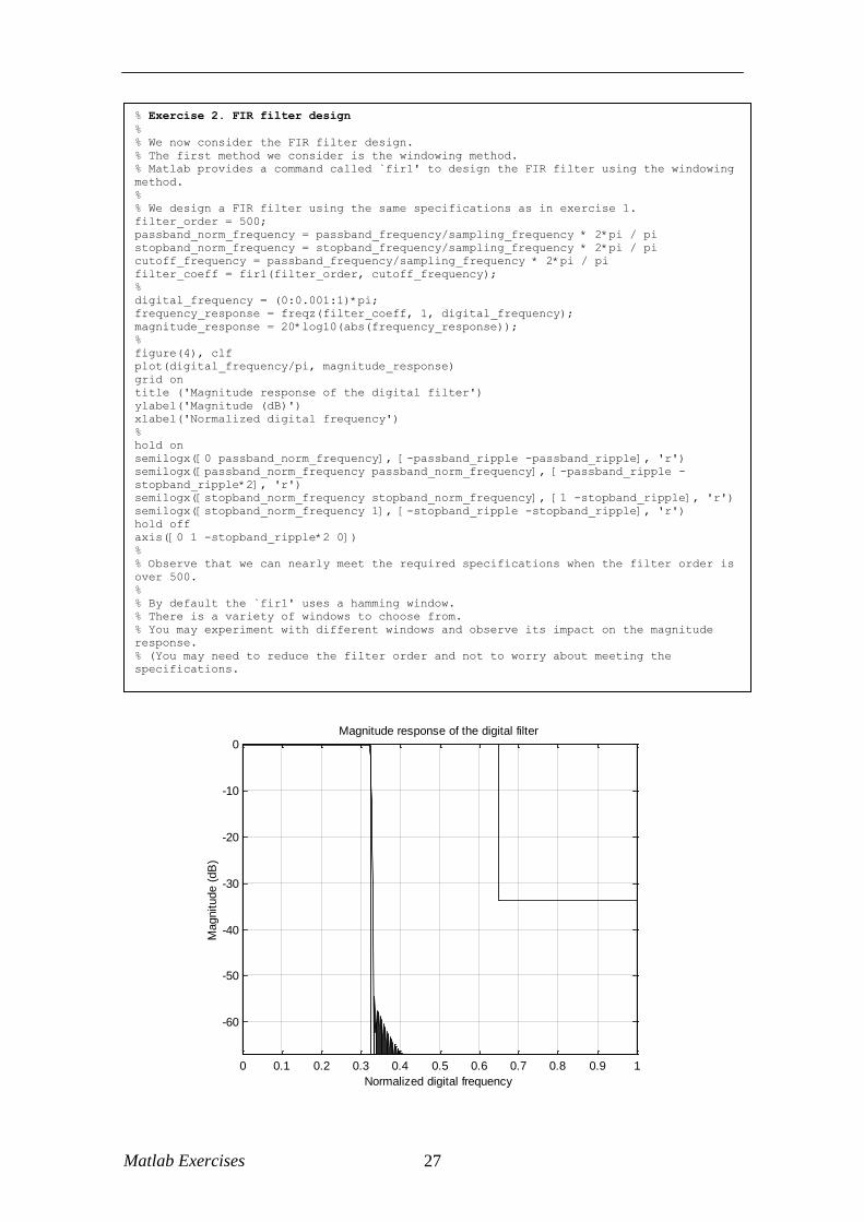
% Exercise 2. FIR filter design

%

% We now consider the FIR filter design.

% The first method we consider is the windowing method.

% Matlab provides a command called `fir1' to design the FIR filter using the windowing

method.

%

% We design a FIR filter using the same specifications as in exercise 1.

filter_order = 500;

passband_norm_frequency = passband_frequency/sampling_frequency * 2*pi / pi

stopband_norm_frequency = stopband_frequency/sampling_frequency * 2*pi / pi

cutoff_frequency = passband_frequency/sampling_frequency * 2*pi / pi

filter_coeff = fir1(filter_order, cutoff_frequency);

%


frequency_response = freqz(filter_coeff, 1, digital_frequency);


%

figure(4), clf

plot(digital_frequency/pi, magnitude_response)

grid on



xlabel('Normalized digital frequency')

%

hold on

semilogx([0 passband_norm_frequency], [-passband_ripple -passband_ripple], 'r')

semilogx([passband_norm_frequency passband_norm_frequency], [-passband_ripple -


semilogx([stopband_norm_frequency stopband_norm_frequency], [1 -stopband_ripple], 'r')

semilogx([stopband_norm_frequency 1], [-stopband_ripple -stopband_ripple], 'r')

hold off

axis([0 1 -stopband_ripple*2 0])

%

% Observe that we can nearly meet the required specifications when the filter order is

over 500.

%

% By default the `fir1' uses a hamming window.

% There is a variety of windows to choose from.

% You may experiment with different windows and observe its impact on the magnitude

response.

% (You may need to reduce the filter order and not to worry about meeting the

specifications.

0 0.1 0.2 0.3 0.4 0.5 0.6 0.7 0.8 0.9 1

-60

-50

-40

-30

-20

-10


Magnitude (

dB

)

Normalized digital frequency

Matlab Exercises 28

0 0.1 0.2 0.3 0.4 0.5 0.6 0.7 0.8 0.9 1

-60

-50

-40

-30

-20

-10


Magnitude (

dB

)

Normalized digital frequency

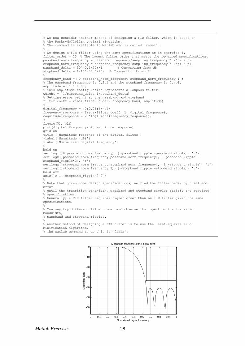
% We now consider another method of designing a FIR filter, which is based on

% the Parks-McClellan optimal algorithm.

% The command is available in Matlab and is called `remez'.

%

% We design a FIR filter using the same specifications as in exercise 1.

filter_order = 13 % The lowest filter order that meets the required specifications.

passband_norm_frequency = passband_frequency/sampling_frequency * 2*pi / pi

stopband_norm_frequency = stopband_frequency/sampling_frequency * 2*pi / pi

passband_delta = 10^(0.1/20)-1 % Converting from dB

stopband_delta = 1/10^(33.5/20) % Converting from dB

%

frequency_band = [0 passband_norm_frequency stopband_norm_frequency 1];

% The passband frequency is 0.2pi and the stopband frequency is 0.4pi.

amplitude = [1 1 0 0];

% This amplitude configuration represents a lowpass filter.

weight = [1/passband_delta 1/stopband_delta]

% Setting error weight at the passband and stopband

filter_coeff = remez(filter_order, frequency_band, amplitude)

%


frequency_response = freqz(filter_coeff, 1, digital_frequency);


%

figure(5), clf

plot(digital_frequency/pi, magnitude_response)

grid on



xlabel('Normalized digital frequency')

%

hold on

semilogx([0 passband_norm_frequency], [-passband_ripple -passband_ripple], 'r')

semilogx([passband_norm_frequency passband_norm_frequency], [-passband_ripple -


semilogx([stopband_norm_frequency stopband_norm_frequency], [1 -stopband_ripple], 'r')

semilogx([stopband_norm_frequency 1], [-stopband_ripple -stopband_ripple], 'r')

hold off

axis([0 1 -stopband_ripple*2 0])

%

% Note that given some design specifications, we find the filter order by trial-and-

error

% until the transition bandwidth, passband and stopband ripples satisfy the required

% specifications.

% Generally, a FIR filter requires higher order than an IIR filter given the same

specifications.

%

% You may try different filter order and observe its impact on the transition

bandwidth,

% passband and stopband ripples.

%

% Another method of designing a FIR filter is to use the least-squares error

minimization algorithm.

% The Matlab command to do this is `firls'.

Matlab Exercises 29


0 2 4 6 8 10 12 14 16 18 200

5

10

15

20

1 2 3 4 5 6 7 8 9 100

5

10

15

20Downsampled signal

0 2 4 6 8 10 12 14 16 18 200

5

10

15

20Upsampled signal

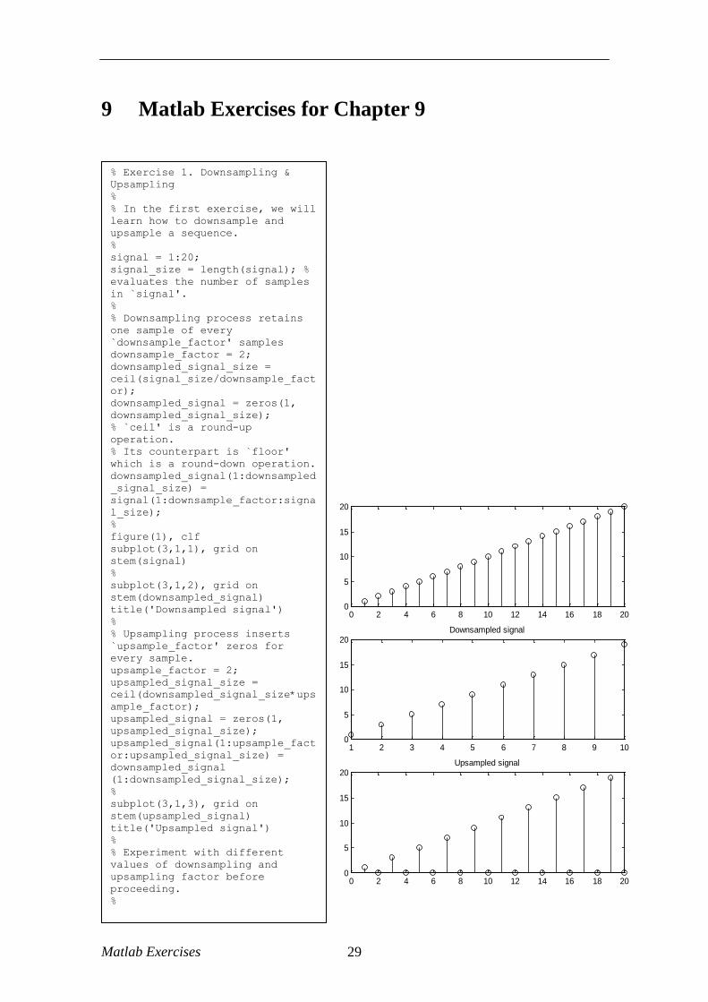
% Exercise 1. Downsampling &

Upsampling

%

% In the first exercise, we will

learn how to downsample and

upsample a sequence.

%

signal = 1:20; % an arbitrary test signal

signal_size = length(signal); %

evaluates the number of samples

in `signal'.

%

% Downsampling process retains

one sample of every

`downsample_factor' samples

downsample_factor = 2;

downsampled_signal_size =

ceil(signal_size/downsample_fact

or);

downsampled_signal = zeros(1,

downsampled_signal_size);

% `ceil' is a round-up

operation.

% Its counterpart is `floor'

which is a round-down operation.

downsampled_signal(1:downsampled

_signal_size) =

signal(1:downsample_factor:signa

l_size);

%

figure(1), clf

subplot(3,1,1), grid on

stem(signal)

%


stem(downsampled_signal)

title('Downsampled signal')

%

% Upsampling process inserts

ùpsample_factor' zeros for

every sample.

upsample_factor = 2;

upsampled_signal_size =

ceil(downsampled_signal_size*ups

ample_factor);

upsampled_signal = zeros(1,

upsampled_signal_size);

upsampled_signal(1:upsample_fact

or:upsampled_signal_size) =

downsampled_signal

(1:downsampled_signal_size);

%


stem(upsampled_signal)

title('Upsampled signal')

%

% Experiment with different

values of downsampling and

upsampling factor before

proceeding.

%

Matlab Exercises 30

0 5 10 15 20 25 30 35 400

5

10

0 20 40 60 80 100 1200

5

10Upsampled signal

0 20 40 60 80 100 1200

5

10Filtered signal

0 2 4 6 8 10 12 14 16 180

5

10Downsampled signal

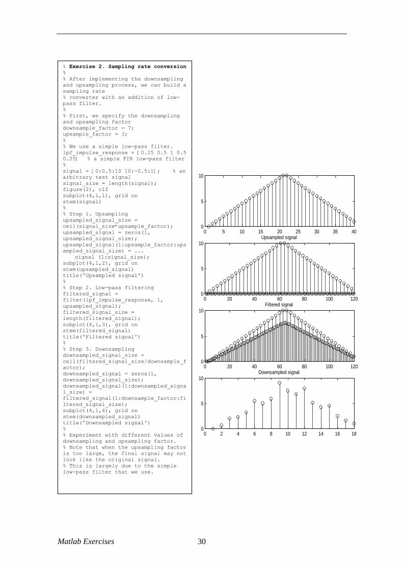
% Exercise 2. Sampling rate conversion

%

% After implementing the downsampling

and upsampling process, we can build a

sampling rate

% converter with an addition of low-

pass filter.

%

% First, we specify the downsampling

and upsampling factor

downsample_factor = 7;

upsample_factor = 3;

%

% We use a simple low-pass filter.

lpf_impulse_response = [0.25 0.5 1 0.5

0.25] % a simple FIR low-pass filter

%

signal = [0:0.5:10 10:-0.5:1]; % an

arbitrary test signal

signal_size = length(signal);

figure(2), clf


stem(signal)

%

% Step 1. Upsampling

upsampled_signal_size =

ceil(signal_size*upsample_factor);

upsampled_signal = zeros(1,

upsampled_signal_size);

upsampled_signal(1:upsample_factor:ups

ampled_signal_size) = ...

signal (1:signal_size);


stem(upsampled_signal)

title('Upsampled signal')

%

% Step 2. Low-pass filtering

filtered_signal =

filter(lpf_impulse_response, 1,

upsampled_signal);

filtered_signal_size =

length(filtered_signal);


stem(filtered_signal)

title('Filtered signal')

%

% Step 3. Downsampling

downsampled_signal_size =

ceil(filtered_signal_size/downsample_f

actor);

downsampled_signal = zeros(1,

downsampled_signal_size);

downsampled_signal(1:downsampled_signa

l_size) =

filtered_signal(1:downsample_factor:fi

ltered_signal_size);


stem(downsampled_signal)

title('Downsampled signal')

%

% Experiment with different values of

downsampling and upsampling factor.

% Note that when the upsampling factor

is too large, the final signal may not

look like the original signal.

% This is largely due to the simple

low-pass filter that we use.

Documents

Matlab Exercises - University of New South WalesMatlab Exercises 2 1 Matlab Exercises for Chapter 1 % Matlab exercises for Chapter 1 % The following codes provide some exercises or