Embed Size (px)
Citation preview

Some Exact Results for the Schršdinger Wave Equation with a
Time Dependent Potential
Joel Campbell
NASA Langley Research Center, MS 488
Hampton, VA 23681
Abstract
The time dependent Schršdinger equation with a time dependent delta function
potential is solved exactly for many special cases. In all other cases the problem can be
reduced to an integral equation of the Volterra type. It is shown that by knowing the wave
function at the origin, one may derive the wave function everywhere. Thus, the problem
is reduced from a PDE in two variables to an integral equation in one. These results are
used to compare adiabatic versus sudden changes in the potential. It is shown that
adiabatic changes in the p otential lead to conservation of the normalization of the
probability density.
02.30Em, 02.60-x, 03.65-w, 61.50-f
https://ntrs.nasa.gov/search.jsp?R=20090034083 2018-09-07T06:14:23+00:00Z

Introduction
Very few cases of the time dependent Schršdinger wave equation with a time
dependent potential can be solved exactly. The cases that are known include the time
dependent harmonic oscillator,[ 1-3] an example of an infinite potential well with a
moving boundary,[4-6] and various other special cases. There remain, however, a large
number of time dependent problems that, at least in principal, can be solved exactly.
One case that has been looked at over the years is the delta function potential. The
author first investigated this problem in the mid 1980s [7] as an unpublished work. This
was later included as part of a PhD thesis dissertation [8] but not published in a journal.
In that work the Schršdinger wave equation with a strength that varies as a function of
time was investigated. That work was more extensive than what we present here in that it
also included the periodic time dependence and a delta function array with time
dependence. In the time that has transpired since then, much (published) work has been
done in relation to time evolution delta function potential problems. Most of that has
focused on the time evolution/propagator derivation of the case of one or more delta
functions with constant amplitude in time. In contrast, this work deals mainly with a
potential with a strength that varies in time.
There are two types of time dependent problems that are commonly investigated. The
problem that has received the most attention over the years is the simple scattering
problem where one seeks what amounts to a steady state solution where the potential has
a periodic dependence on time. In the case of the delta function potential, this problem
was investigated where the strength varied sinusoidally in time[9] . Using Floquet
formalism, they were able to derive a transmission coefficient as a function of driving
frequency and amplitude. Other examples of scattering problems involving delta function
2

potentials also exist in the literature [10]. The actual solutions, however, are simple plane
waves.
The other time dependent problem is where one starts with an initial state and allows
that to evolve in time. These are the diffusive solutions to the Schršdinger wave equation.
This and the closely related problem of finding the propagator have been investigated in
some depth in relation to the one or more delta function potential [ 11-16] . Out of those
cases cited only one of them involves a potential with true time dependence [13] and that
is the case of two delta functions that move apart from one another at constant velocity.
There are two common approaches one may use. One method is using a path integral of
the Feynma n type and the other is using Laplace transforms. We use the latter though the
two methods are closely related.
Formulation of the Problem
We would like to solve the Schršdinger equation with a time dependent potential,
xx + 2c(t)(x) = i
t
(1)0, x ±
By integrating Equation 1 over the discontinuity at x=0, we find that the problem
reduces to,
xx = i t
x (0+ , t)—yf- x(0, t) = 2c ( t)W(0, t ) (2)
0, x ±
This is just the case of zero potential with an additional time dependent boundary
condition. If we restrict ourselves to t>0, we may take the Laplace transform of Equation
2
xx = i$ i(x,0)(3)
tVx (0+ , $) — tVx (0- , $) = 2L[c(t)Vf(0, t)]

We now solve Equation 3. However, we must consider the homogeneous solution in
order to satisfy the cusp condition at the origin. The solution is
is x)+ 21 is
J dx' exp( i is x — x ' )y^(x',0)W(x , s) = a(s) exp( i
where a(s) is an arbitrary function of s, yet to be determined. By applying the cusp
condition at the origin to Equation 2.4 we find
x(0+, s) — x(0, s) = 2i isa(s) = 2L[c(t)(0, t)]
=> a(s) = L[c(t)yf(0, t)]
i is
We now set x=0 in Equation 4 and use the results of Equation 5 to find
y (0, s) = L[c(t)yi(0, t)]
+ 1 dx 'exp( i is l x ' )y1(x',0)
i is 2 is _
Using the convolution theorem for Laplace transforms [17], we invert Equation 6 to
find
1V(0, t) —. 1 t
dt' c( t ')(0' t ')
= 1
J dx 'exp i (x ')
2
x' ,0) (7)a i 0 t— t 2 -6-c _ 4 t
Equation 7 is a Volterra integral equation that determines the wave function at the
origin. Once the wave function at the origin is known, one may find the wave function
everywhere by inverting Equation 4 which has the result
2
(
) 1t ' c ( t ')yi(0, t ') x 2
1J
(x — x ') )x, t = dt exp i + J dx'ex i (x ',0 (8)
i i 0 t— t' 4( t — t ') 2 i7t _ 4 t
Equations 7 and 8 completely determine the problem. As we can see knowing the wave
function at the origin is equivalent to knowing the wave function everywhere.
(4)
(5)
(6)
4
Some Specific Cases
Derivation of the Propagator for Constant c and Jumps
In some situations it is advantageous to represent the solution in the form,
(x , t) = dx ' G(x , x' , t)(x',0) (9)
where G is the propagator. To find the propagator, we use Equations 5 and 6 to find,
a(s) = cyf (0, s) = — c 1 1 r dx 'exp( i is I x ' I )(x',0 ) (10)
i is 2 ss + ic _
By Equations 4 and 10, we find,
_ c exp( i is(x l + I x ' I)) exp( i is l x — x ' )G(x , x' , s) = + (11)
2 s(s + ic) 2 is
By making the substitution k= is we see this is the same propagator found using the
Feynman approach [ 11 ] . We may now invert Equation 11 to obtain,
G(x , x' , t) = — 2 exp[c ( x l + x ' ) + ic 2t] erfc c it +
2
+
it +
(12)1 ( — x ')
2
ex ix2 it 4 t
Non-adiabatic Jumps
Although this example is for c=constant, we may use this to generate a solution for a
sudden, non-adiabatic jump in the potential. This is quite simple to do. If we choose c=-
c0 , where c0 is a positive real number and take (x, 0 ) = c0 exp( c0 x) as the initial
state, the system evolves with a probability density that doesn't change in time except for
phase. That is because we have chosen the bound state for the attractive potential case.
One way to model a sudden jump is to chose an initial state of
5

(x, 0 ) = c0 exp( c0 x) , but let it evolve thereafter with c=-c', where c'>0. It can be
shown that in this case [8],
2c c o
yf(x,t)^ exp(-c x)exp(ic 2 t),t (13)c
0+c
The total probability of it radiating away is,
2
1-( Vf(x,t) 2
/=
c 0 - c , t (14)c 0 +c
We see that sudden changes in potential lead to irreversible changes in the normalization
of the probability density as we would expect.
Adiabatic Limit
Interestingly enough, we may also generate the adiabatic case as well using similar
reasoning. The probability of it remaining in the bound state after one jump is
(x,t) \2=
4c0c
2 , t °O (15)
(c 0+c ' )
Lets suppose now we break it up into two steps. We first take a small half step, let it
evolve for a long time, then take a second step and let it evolve again. The result is
(x,t) 2
= 4c 0c
1 2 4c
1c
2 2
, t (16)(c 0 +c 1 ) (c 1 +c
2 )
Here, cn = c0 + n (c '— c0 ) /2. After N such steps we have,
'I` 7^7 \N- 1
( Y' (x, t, ) I 2 / = 4Nri
4cncn+ 1
2 ,t, (17)°On=0 (c n +cn+ 1 )
where cn = c0 + n (c ' — c0 ) / N. The result is
6

(x,t,N) 2 =
4 c° (c '+ c
° (- 1 + N))N I'(a1 - 1 + N ) 11'( a2 — 1 + N ) 11'( a3 )
2 (18)
( c '+ c°(-1 + 2N ))
2 ][- (a1) I (a2)
IF (a 3 — 1 + N) ,t
)
where
a1 = 2 + c0 N,
c I c0
a2 = 1 + I
c0 N, (19)
c— c0
3 c0 N.a3 = — + ^2 c '— c0
By taking the limit as N approaches infinity we find
Nim (Yf
(x,tN)^ 2
) =1, t . (20)
This implies the probability of the particle radiating away is 0. Thus, for adiabatic
changes in the potential, the normalization of the probability density is conserved, as we
would infer from the Born-Fock theorem [18] on the conservation of quantum numbers.
Solution for c Linear in Time
We now consider a potential that has the following form,
c(t) = c 0 , t < 0
c(t) = c0 — t , t > 0
Here, a is a real number. We take the bound state for c=-c 0 as the initial condition,
which in this case is ( x ,°) = c° exp( c° x) , where and c0 are real constants and
c0>0. By Equation 6 and using L[ t f(t)]=-d (L [f(t))]/ds, we find,
yfs (°, s) — 1 (i is + c ° )yi(°, s) = i c ° (22)
a a c° — i is
(21)
7
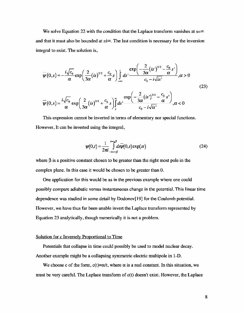
We solve Equation 22 with the condition that the Laplace transform vanishes at s= oo
and that it must also be bounded at ±i oo . The last condition is necessary for the inversion
integral to exist. The solution is,
2'
3/2 Co'
s exp —(is) — C s
yf (0, s ) = — i c
0 exp 23a a
( is )3/2 + °̂ s f ds'
3a a, a > 0
a ( ) _ i co —
i is^
(23)
r l 2 3/2exp( is s'
icJ
uf (0, s ) =
0 exp l 23a a(is ) 3 /z + a
sJ
f ds,, < 0
a 3 a J Js c0 — i is'
This expression cannot be inverted in terms of elementary nor special functions.
However, It can be inverted using the integral,
i1
+ p
(0, t) =
ds (0, s)exp(st ) (24)2 i
i +
where P is a positive constant chosen to be greater than the right most pole in the
complex plane. In this case it would be chosen to be greater than 0.
One application for this would be as in the previous example where one could
possibly compare adiabatic versus instantaneous change in the potential. This linear time
dependence was studied in some detail by Dodonov[19] for the Coulomb potential.
However, we have thus far been unable invert the Laplace transform represented by
Equation 23 analytically, though numerically it is not a problem.
Solution for c Inversely Proportional to Time
Potentials that collapse in time could possibly be used to model nuclear decay.
Another example might be a collapsing symmetric electric multipole in 1-D.
We choose c of the form, c(t)=/t, where a is a real constant. In this situation, we
must be very careful. The Laplace transform of c(t) doesn't exist. However, the Laplace
8

transform of c(t) (0,t) does exist if we choose an initial condition that vanishes at the
origin. With this restriction in mind, we proceed with the problem. We first use the
identity,
L [1 t f (t) , s] = ds ' L[ f (t) , s'] (25)
s
By Equations 25 and 6 we find
t (0, s) = a
ds ' y (0, s ') + 1
dx 'exp( i is x ')V(x ',0) (26)i is s i4is —
Let,
u(s) = f ds ' Yf (0, s ') (27)s
Then by Equations 26 and 27 we find
us + a u = — 1 j dx 'exp( i is x' )(x ',0) (28)i is 2 is
After solving Equation 28 we find
uexp( i is x ')
Y/(x ' ,0)—dx x ' + 2 i
By Equation 29 we find,
1 ^ x' exp( i is x ')yi(0, s) = ^ dx yi(x ',0) (30)2 is _ I x' + 2i
We may now invert Equation 30 to find,
t/i(0, t) = 1i dx'
x ' exp i (
x ')2
(x ',0) (31)2 it x' + 2 i 4 t
We now seek (x,t). To find this quantity, we first write,
(29)
(x , t) = dx ' G(x , x' , t)(x',0) (32)
9

To find G, we use the results of Equations 30, 27, 5, and 4 to find,
G(x , x' , s) = 1 — 2 ia
exp( i is(x + x' )) + exp( i is(x — x' )) (33)2 is x' + 2 i
We may now invert this expression to find,
2 2
(34)1 2 ia (x + x ' ) (x — x ')
G(x , x' , t) = — exp i + exp i2 it x' + 2 i 4 t 4 t
Solution for c with an Exponential Dependence on Time
In this case we choose c(t)=-c0 for t<0 and c(t)=-c0 + exp(-t) for t>0, where c0 is
real such that c0>0, P is real, and >0. We choose the bound state for c(t)=-c 0 as the
initial condition where (x, 0 ) = c0 exp( c0 x) . This represents a type of impulse. One
can imagine the constant attractive bound state case, where at t=0, the potential jumps to -
c0+b, then quickly falls back to -c0. This could represent a model for stimulated
emission.
We use the shift formula for Laplace transforms, which is given by,
L[exp(at) f (t) ,s] = L [f (t) ,s — a]
By Equations 35 and 6 we find,
Y/(0, s) = c 0
2 —
ir̂. VI(0, s + a)
s—ic 0 s—vlc 0
To obtain a solution, we could iterate this expression repeatedly to obtain the series
solution,
y (0, s) = nan(s) (37)n=0
(35)
(36)
10

But since we already know the form of the series, we may substitute Equation 37
directly into Equation 36. After doing this and solving for the a's by equating terms with
like powers of , we find an(s) is given by
c0
an (s ) = 2 , n = 0
s — ic0
.^i)
n (38)c 0
n _1 1an s
( ) = , n > 0s + nic 02 j=0 s + jic0
Discussion
It was shown that the time dependent Schršdinger equation with a time dependent
delta function potential can be solved exactly in many special cases. We were able to
show that, in contrast to the case of sudden change, the adiabatic change in the potential
leads to a conservation in the normalization of the probability density of the bound state.
This is a rather significant result because it proves the system is reversible to within a
phase factor if the change is slow enough.
The periodic case and multi-delta function case was excluded for the sake of brevity
and because they deserve a separate treatment due to the complexity of the solutions. The
case of the sinusoidal time dependent potential can be treated in a similar manner as the
exponential time dependent potential by representing the sine function as a sum of
complex exponentials. Those two cases have also been treated elsewhere in a different
context. As stated earlier the scattering problem was solved for the delta function with a
strength that varied periodically in time [9] in as much as they were able to derive a
transmission coefficient. We treated that same case as an initial value problem a decade
before [8]. In the case of the multi-delta-function potential, this has also been recently
treated in the literature [14,15] in the case of constant in time delta function potentials
11

and also in the case of delta function potentials moving with constant speed [ 13] . We also
treated that case more than a decade before [8] for the case where the strength varies in
time.
12
References
[1] P. G. L. Leach 1977, Journal of Mathematical Physics 18, 1608.
[2] P. G. L. Leach 1977, Journal of Mathematical Physics 18, 1902.
[3] P. G. L. Leach 1978, Journal of Mathematical Physics 19, 446.
[4] A. Munier, J. R. Burgan, M. Feix, E. Fijalkow 1981, Journal of MathematicalPhysics, 22, 1219.
[5] V.V. Dodonov et al 1993, Quantum particle in a box with moving walls, Journal ofMathematical Physics, 34, 3391
[6] Alberto Devotot and Bojan Pomorisac 1992, Diffusion-like solutions of theSchrodinger equation for a time-dependent potential well, J. Phys. A, 25, 241
[7] Joel Campbell and Bill Sutherland 1985, Quantum mechanical treatment of a timedependent potential (unpublished).
[8] Joel Campbell, Topics in Mathematical Physics, PhD Thesis dissertation, Universityof Utah, 12/91
[9] D. F. Martinez and L. E. Reichl 2001, Transmission properties of the oscillating delta-function potential, Phys. Rev. B, 64, 245315
[10] K.J. LaGattuta 1994, Laser assisted scattering from a one-dimensional delta-functionpotential: An exact solution, Phys. Rev. A. 49 ,1745
[11] S.M. Blinder 1988, Greens function and propagator for the one-dimensional deltafunction potential, Phys. Rev. A, 37, 973
[12] D.K. Park 1996, Proper incorporation of the self-adjoint extension methodto the Green function formalism: one-dimensional delta-function potential case, J. PhysA, 29, 6407
[13] G. Scheitler and M. Kleber 1990, Propagator for two dispersing delta-functionpotentials, Phys. Rev. A, 42, 55
[ 14] Ilaria Cacciari and Paolo Moretti 2006, Propagator for finite range potentials,Journal of Mathematical Physics, 47, 12210912210
[15] Ilaria Cacciari and Paolo Moretti 2006, Propagator for the double delta potential,Physics Letters A, 359, 396
13

[16] V.V. Dodonov, V.I. Man'ko, D.E. Nikonov, Exact propagators fortime-dependent Coulomb, delta and other potentials.Phys. Lett. A 162 (1992), 5, 359-364.
[17] M. Abramowitz and I. Stegun 1970, Handbook of Mathematical Functions. Eq.29.2.8, Dover Publications
[18] M. Born and V. Fock 1928, Beweis des Adiabatensatzes,Zeitschrift fŸr Physik 51 S.165-180
[19] V.V. Dodonov, V.I. Man'ko and D.L. Ossipov, in: Proc. Lebedev Phys. Inst. Aead.Sci. USSR, Vol. 176 (Nova Science Publishers, Commack, NY, 1988) p. 61.
14