Embed Size (px)
Citation preview
The stochastic wave equation
by
Robert C. Dalang1
Abstract. These notes give an overview of recent results concerning the non-linearstochastic wave equation in spatial dimensions d ≥ 1, in the case where the drivingnoise is Gaussian, spatially homogeneous and white in time. We mainly address issuesof existence, uniqueness and Holder-Sobolev regularity. We also present an extensionof Walsh’s theory of stochastic integration with respect to martingale measures thatis useful for spatial dimensions d ≥ 3.
Key words and phrases. Stochastic partial differential equations, sample pathregularity, spatially homogeneous random noise, wave equation.
MSC 2000 Subject Classifications. Primary 60H15; Secondary 60J45, 35R60,35L05.
1Partially supported by the Swiss National Foundation for Scientific Research.

1 Introduction
The stochastic wave equation is one of the fundamental stochastic partial differentialequations (s.p.d.e.’s), of hyperbolic type. The behavior of its solutions is signifi-cantly different from those of solutions to other s.p.d.e.’s, such as the stochastic heatequation. In this introductory section, we present two real-world examples that canmotivate the study of this equation, even though in neither case is the mathematicaltechnology sufficiently developed to answer the main questions of interest. It is how-ever pleasant to have such examples in order to motivate the development of rigorousmathematics.
Example 1: The motion of a strand of DNA
A DNA molecule can be view as a long elastic string, whose length is essentiallyinfinitely long compared to its diameter. We can describe the position of the stringby using a parameterization defined on R+ × [0, 1] with values in R3:
~u(t, x) =
u1(t, x)u2(t, x)u3(t, x)
.Here, ~u(t, x) is the position at time t of the point labelled x on the string, wherex ∈ [0, 1] represents the distance from this point to one extremity of the string if thestring were straightened out. The unit of length is chosen so that the entire stringhas length 1.
A DNA molecule typically “floats” in a fluid, so it is constantly in motion, justas a particle of pollen floating in a fluid moves according to Brownian motion. Themotion of the particle can be described by Newton’s law of motion, which equates thesum of forces acting on the string with the product of the mass and the acceleration.Let µ = 1 be the mass of the string per unit length. The acceleration at position xalong the string, at time t, is
∂2~u
∂t2(t, x),
and the forces acting on the string are mainly of three kinds: elastic forces ~F1, whichinclude torsion forces, friction due to viscosity of the fluid ~F2, and random impulses~F3 due the the impacts on the string of the fluid’s molecules. Newton’s equation ofmotion can therefore be written
1 · ∂2~u
∂t2= ~F1 − ~F2 + ~F3.
This is a rather complicated system of three stochastic partial differential equa-tions, and it is not even clear how to write down the torsion forces or the friction term.
1
Elastic forces are generally related to the second derivative in the spatial variable,and the molecular forces are reasonably modelled by a stochastic noise term.
The simplest 1-dimensional equation related to this problem, in which one onlyconsiders vertical displacement and forgets about torsion, is the following one, inwhich u(t, x) is now scalar valued:
∂2u
∂t2(t, x) =
∂2u
∂x2(t, x)−
∫ 1
0k(x, y)u(t, y) dy + F (t, x), (1.1)
where the first term on the right hand side represents the elastic forces, the secondterm is a (non-local) friction term, and the third term F (t, y) is a Gaussian noise,with spatial correlation k(·, ·), that is,
E(F (t, x) F (s, y)) = δ0(t− s) k(x, y),
where δ0 denotes the Dirac delta function. The function k(·, ·) is the same in thefriction term and in the correlation.
Why is the motion of a DNA strand of biological interest? When a DNA strandmoves around and two normally distant parts of the string get close enough together,it can happen that a biological event occurs: for instance, an enzyme may be released.Therefore, some biological events are related to the motion of the DNA string. Somemathematical results for equation (1.1) can be found in [18]. Some of the biologicalmotivation can be found in [7].
Example 2: The internal structure of the sun
The study of the internal structure of the sun is an active area of research. Oneimportant international project is known as Project SOHO [8]. Its objective was touse measurements of the motion of the sun’s surface to obtain information about theinternal structure of the sun. Indeed, the sun’s surface moves in a rather complexmanner: at any given time, any point on the surface is typically moving towards oraway from the center. There are also waves going around the surface, as well as shockwaves propagating through the sun itself, which cause the surface to pulsate.
A question of interest to solar geophysicists is to determine the origin of theseshock waves. One school of thought is that they are due to turbulence, but thelocation and intensities of the shocks are unknown, so a probabilistic model can beconsidered.
A model that was proposed by P. Stark of U.C. Berkeley is that the main sourceof shocks is located in a spherical zone inside the sun, which is assumed to be a ballof radius R. Assuming that the shocks are randomly located on this sphere, theequation for the pressure variations throughout the sun would be
∂2u
∂t2(t, x) = c2(x) ρ0(x)
(~∇ ·
(1
ρ0(x)~∇u)− ~∇ · ~F (t, x)
), (1.2)
2

where x ∈ B(0, R), the ball centered at the origin with radius R, c2(x) is the speed of
wave propagation at position x, ρ0(x) is the density at position x and ~F (t, x) modelsthe shock that originates at time t and position x.
A model for ~F that corresponds to the description of the situation would be 3-dimensional Gaussian noise concentrated on the sphere ∂B(0, r), where 0 < r < R.
A possible choice of the spatial correlation for the components of ~F would be
δ(t− s) f(x · y),
where x · y denotes the Euclidean inner product. A problem of interest is to estimater from the available observations of the sun’s surface. Some mathematical resultsrelevant to this problem are developed in [3].
2 The stochastic wave equation
Equation (1.2) is a wave equation in vector form. The (simpler) real-valued stochasticwave equation, that we will be studying in these notes, reads as follows:
(∂2u∂t2
−∆u)
(t, x) = σ(t, x, u(t, x)) F (t, x) + b(t, x, u(t, x), (t, x) ∈ [0, t]× Rd
u(0, x) = v0(x),∂u
∂t(0, x) = v0(x),
(2.1)where F (t, x) is a Gaussian noise, which we take to be space-time white noise for themoment, and σ, b : R+ × Rd × R → R are functions that satisfy standard properties,such as being Lipschitz in the third variable. The term ∆u denotes the Laplacian ofu in the x-variables.
Mild solutions of the stochastic wave equation
It is necessary to specify the notion of solution to (2.1) that we are considering.We will mainly be interested in the notion of mild solution, which is the followingintegral form of (2.1):
u(t, x) =∫[0,t]×Rd
G(t− s, x− y) [σ(s, y, u(s, y)) F (s, y) + b(s, y, u(s, y))] ds dy
+
(d
dtG(t) ∗ v0
)(x) + (G(t) ∗ v0)(x). (2.2)
In this equation, G(t − s, x − y) is the Green’s function of (2.1), which we discussnext, and ∗ denotes convolution in the x-variables. For the term involving F (s, y), anotion of stochastic integral is needed, that we will discuss later on.
Green’s function of a p.d.e.
3
We consider first the case of an equation with constant coefficients. Let L be apartial differential operator with constant coefficients. A basic example is the waveoperator
Lf =∂2f
∂t2−∆f.
Then there is a (Schwartz) distribution G ∈ S ′(R+ × Rd) such that the solution ofthe p.d.e.
Lu = ϕ, ϕ ∈ S(Rd),
isu = G ∗
(t,x) ϕ
where ∗(t,x) denotes convolution in the (t, x)-variables. We recall that S(Rd) denotes
the space of smooth test functions with rapid decrease, and S ′(R+ ×Rd) denotes thespace of tempered distributions [13].
When G is a function, this convolution can be written
u(t, x) =∫
R+×RdG(t− s, x− y)ϕ(s, y) ds dy.
We note that this is the solution with vanishing initial conditions.In the case of an operator with non-constant coefficients, such as
Lf =∂2f
∂t2+ 2c(t, x)
∂f
∂t+∂2f
∂x2(d = 1),
the Green’s function has the form G(t, x ; s, y) and the solution of
Lu = ϕ
is given by the expression
u(t, x) =∫
R+×RdG(t, x ; s, y)ϕ(s, y) ds dy.
Example 2.1 The heat equation. The partial differential operator is
Lu =∂u
∂t−∆u, d ≥ 1,
and the Green’s function is
G(t, x) = (2πt)−d/2 exp
(−|x|
2
2t
).
This function is smooth except for a singularity at (0, 0).
4
Example 2.2 The wave equation. The partial differential operator is
Lu =∂2u
∂t2−∆u.
The form of the Green’s function depends on the dimension d. We refer to [16] ford ∈ 1, 2, 3 and to [6] for d > 3. For d = 1, it is
G(t, x) =1
21|x|<t,
which is a bounded but discontinuous function. For d = 2, it is
G(t, x) =1√2π
1√t2 − |x|2
1|x|<t.
This function is unbounded and discontinuous. For d = 3, the “Green’s function” is
G(t, dx) =1
4π
σt(dx)
t,
where σt is uniform measure on ∂B(0, t), with total mass 4πt2. In particular, G(t,R3) =t. This Green’s function is in fact not a function, but a measure. Its convolution witha test function ϕ is given by
(G ∗ ϕ)(t, x) =1
4π
∫ t
0ds∫
∂B(0,s)ϕ(t− s, x− y)
σs(dy)
s
=1
4π
∫ t
0ds s
∫∂B(0,1)
ϕ(t− s, x− sy)σ1(dy).
Of course, the meaning of an expression such as∫[0,t]×Rd
G(t− s, x− y)F (ds, dy)
where G is a measure and F is a Gaussian noise, is now unclear: it is certainly outsideof Walsh’s theory of stochastic integration [9].
In dimensions greater than 3, the Green’s function of the wave equation becomeseven more irregular. For d ≥ 4, set
N(d) =
d−32
if d is odd,
d−22
if d is even.
For d even, set
σdt (dx) =
1√t2 − |x|2
1|x|<t dx,
5
and for d odd, let σdt (dx) be the uniform surface measure on ∂B(0, t) with total mass
td−1. Then for d odd, G(t, x) can formally be written
G(t, x) = cd
(1
s
∂
∂s
)N(d) (σd
s
s
)ds,
that is, for d odd,
(G ∗ ϕ)(t, x) = cd
∫ t
0ds
(1
r
∂
∂r
)N(d) (∫Rdϕ(t− s, x− y)
σdr (dy)
r
) ∣∣∣∣∣r=s
while for d even,
(G ∗ ϕ)(t, x) = cd
∫ t
0ds
(1
r
∂
∂r
)N(d)∫
B(0,r)ϕ(t− s, x− y)
dy√r2 − |y|2
∣∣∣∣∣r=s
.
The meaning of∫[0,t] G(t− s, x− y) F (ds, dy) is even less clear in these cases!
The case of spatial dimension one
Existence and uniqueness of the solution to the stochastic wave equation in spatialdimension 1 is covered in [17, Exercise 3.7 p.323]. It is a good exercise that we leaveto the reader.
Problem 1. Establish existence and uniqueness of the solution to the non-linear waveequation on [0, t]× R, driven by space-time white noise :
∂2u
∂t2− ∂2u
∂x2= σ(u(t, x)) W (t, x)
with initial conditions
u(0, ·) =∂u
∂x(0, ·) ≡ 0.
The solution uses the following standard steps, which also appear in the study of thesemilinear stochastic heat equation (see [17] and [9]):
- define the Picard iteration scheme;- establish L2-convergence using Gronwall’s lemma;- show existence of higher moments of the solution, using Burkholder’s inequality
E(|Mt|p) ≤ cpE(〈M〉p/2t ); (2.3)
- establish Holder continuity of the solution.
It is also a good exercise to do the following calculation.
6
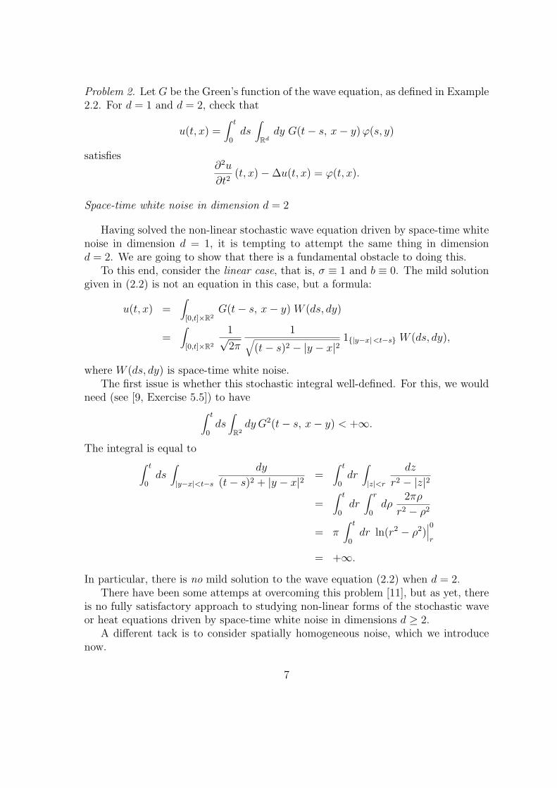
Problem 2. Let G be the Green’s function of the wave equation, as defined in Example2.2. For d = 1 and d = 2, check that
u(t, x) =∫ t
0ds∫
Rddy G(t− s, x− y)ϕ(s, y)
satisfies∂2u
∂t2(t, x)−∆u(t, x) = ϕ(t, x).
Space-time white noise in dimension d = 2
Having solved the non-linear stochastic wave equation driven by space-time whitenoise in dimension d = 1, it is tempting to attempt the same thing in dimensiond = 2. We are going to show that there is a fundamental obstacle to doing this.
To this end, consider the linear case, that is, σ ≡ 1 and b ≡ 0. The mild solutiongiven in (2.2) is not an equation in this case, but a formula:
u(t, x) =∫[0,t]×R2
G(t− s, x− y) W (ds, dy)
=∫[0,t]×R2
1√2π
1√(t− s)2 − |y − x|2
1|y−x|<t−s W (ds, dy),
where W (ds, dy) is space-time white noise.The first issue is whether this stochastic integral well-defined. For this, we would
need (see [9, Exercise 5.5]) to have∫ t
0ds∫
R2dy G2(t− s, x− y) < +∞.
The integral is equal to∫ t
0ds∫|y−x|<t−s
dy
(t− s)2 + |y − x|2=
∫ t
0dr∫|z|<r
dz
r2 − |z|2
=∫ t
0dr∫ r
0dρ
2πρ
r2 − ρ2
= π∫ t
0dr ln(r2 − ρ2)
∣∣∣0r
= +∞.
In particular, there is no mild solution to the wave equation (2.2) when d = 2.There have been some attemps at overcoming this problem [11], but as yet, there
is no fully satisfactory approach to studying non-linear forms of the stochastic waveor heat equations driven by space-time white noise in dimensions d ≥ 2.
A different tack is to consider spatially homogeneous noise, which we introducenow.
7

3 Spatially homogeneous Gaussian noise
Let Γ be a non-negative and non-negative definite tempered measure on Rd, so thatΓ(dx) ≥ 0, ∫
RdΓ(dx) (ϕ ∗ ϕ)(x) ≥ 0, for all ϕ ∈ S(Rd),
where ϕ(x)def= ϕ(−x), and there exists r > 0 such that∫
RdΓ(dx)
1
(1 + |x|2)r<∞.
According to the Bochner-Schwartz theorem [13], there is a nonnegative measureµ on Rd whose Fourier transform is Γ: we write Γ = Fµ. By definition, this meansthat for all ϕ ∈ S(Rd), ∫
RdΓ(dx)ϕ(x) =
∫Rdµ(dη) Fϕ(η) .
We recall that the Fourier transform of ϕ ∈ S(Rd) is
Fϕ(η) =∫
Rdexp(−i η · x) ϕ(x) dx,
where η ·x denotes the Euclidean inner product. The measure µ is called the spectralmeasure.
Definition 3.1 A spatially homogeneous Gaussian noise that is white in time is anL2(Ω,F , P )−valued mean zero Gaussian process(
F (ϕ), ϕ ∈ C∞0 (R1+d)
)such that
E(F (ϕ)F (ψ)) = J(ϕ, ψ),
whereJ(ϕ, ψ)
def=∫
R+
ds∫
RdΓ(dx) (ϕ(s, ·) ∗ ψ(s, ·))(x).
In the case where the covariance measure Γ has a density, so that Γ(dx) = f(x) dx,then it is immediate to check that J(ϕ, ψ) can be written as follows:
J(ϕ, ψ) =∫
R+
ds∫
Rddx∫
Rddy ϕ(s, x) f(x− y)ψ(s, y).
Using the fact that the Fourier transform of a convolution is the product of the Fouriertransforms, this can also be written
J(ϕ, ψ) =∫
R+
ds∫
Rdµ(dη)Fϕ(s)(η)Fψ(s)(η).
Informally, one often writes
E(F (t, x)F (s, y)) = δ0(t− s) f(x− y).
8
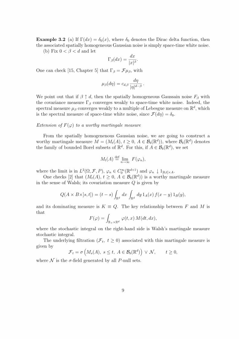
Example 3.2 (a) If Γ(dx) = δ0(x), where δ0 denotes the Dirac delta function, thenthe associated spatially homogeneous Gaussian noise is simply space-time white noise.
(b) Fix 0 < β < d and let
Γβ(dx) =dx
|x|β.
One can check [15, Chapter 5] that Γβ = Fµβ, with
µβ(dη) = cd,βdη
|η|d−β.
We point out that if β ↑ d, then the spatially homogeneous Gaussain noise Fβ withthe covariance measure Γβ converges weakly to space-time white noise. Indeed, thespectral measure µβ converges weakly to a multiple of Lebesgue measure on Rd, whichis the spectral measure of space-time white noise, since F(dη) = δ0.
Extension of F (ϕ) to a worthy martingale measure
From the spatially homogenenous Gaussian noise, we are going to construct aworthy martingale measure M = (Mt(A), t ≥ 0, A ∈ Bb(Rd)), where Bb(Rd) denotesthe family of bounded Borel subsets of Rd. For this, if A ∈ Bb(Rd), we set
Mt(A)def= lim
n→∞F (ϕn),
where the limit is in L2(Ω,F , P ), ϕn ∈ C∞0 (Rd+1) and ϕn ↓ 1[0,t]×A.
One checks [2] that (Mt(A), t ≥ 0, A ∈ Bb(Rd)) is a worthy martingale measurein the sense of Walsh; its covariation measure Q is given by
Q(A×B×]s, t]) = (t− s)∫
Rddx
∫Rddy 1A(x) f(x− y) 1B(y),
and its dominating measure is K ≡ Q. The key relationship between F and M isthat
F (ϕ) =∫
R+×Rdϕ(t, x)M(dt, dx),
where the stochastic integral on the right-hand side is Walsh’s martingale measurestochastic integral.
The underlying filtration (F t, t ≥ 0) associated with this martingale measure isgiven by
F t = σ(Ms(A), s ≤ t, A ∈ Bb(Rd)
)∨ N , t ≥ 0,
where N is the σ-field generated by all P -null sets.
9
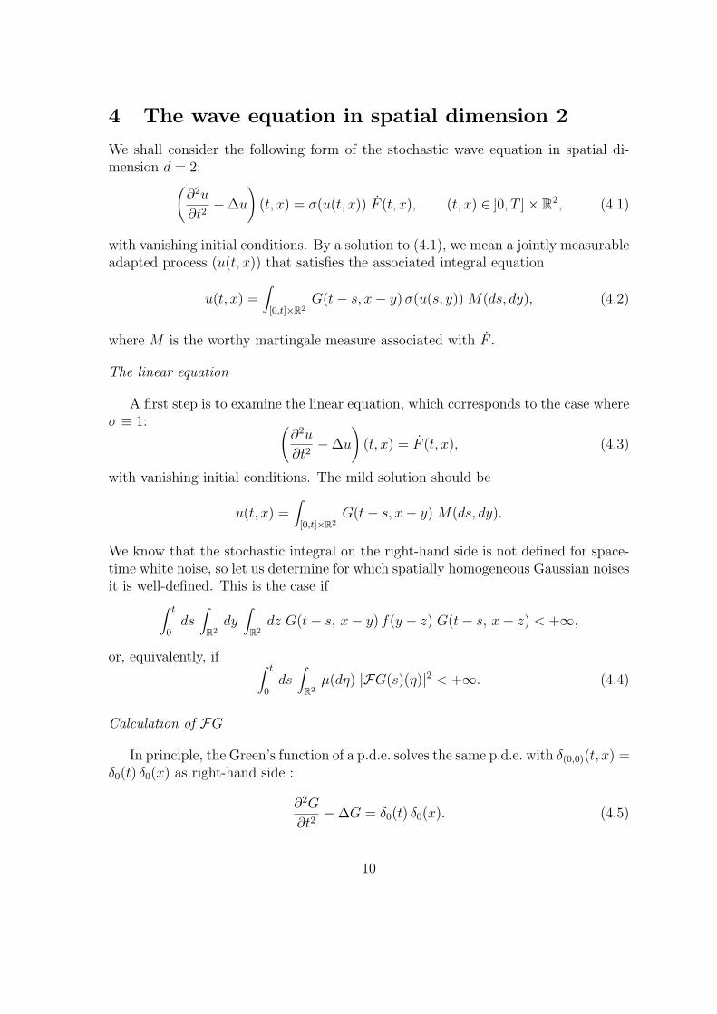
4 The wave equation in spatial dimension 2
We shall consider the following form of the stochastic wave equation in spatial di-mension d = 2:(
∂2u
∂t2−∆u
)(t, x) = σ(u(t, x)) F (t, x), (t, x) ∈ ]0, T ]× R2, (4.1)
with vanishing initial conditions. By a solution to (4.1), we mean a jointly measurableadapted process (u(t, x)) that satisfies the associated integral equation
u(t, x) =∫[0,t]×R2
G(t− s, x− y)σ(u(s, y)) M(ds, dy), (4.2)
where M is the worthy martingale measure associated with F .
The linear equation
A first step is to examine the linear equation, which corresponds to the case whereσ ≡ 1: (
∂2u
∂t2−∆u
)(t, x) = F (t, x), (4.3)
with vanishing initial conditions. The mild solution should be
u(t, x) =∫[0,t]×R2
G(t− s, x− y) M(ds, dy).
We know that the stochastic integral on the right-hand side is not defined for space-time white noise, so let us determine for which spatially homogeneous Gaussian noisesit is well-defined. This is the case if∫ t
0ds∫
R2dy
∫R2dz G(t− s, x− y) f(y − z) G(t− s, x− z) < +∞,
or, equivalently, if ∫ t
0ds∫
R2µ(dη) |FG(s)(η)|2 < +∞. (4.4)
Calculation of FG
In principle, the Green’s function of a p.d.e. solves the same p.d.e. with δ(0,0)(t, x) =δ0(t) δ0(x) as right-hand side :
∂2G
∂t2−∆G = δ0(t) δ0(x). (4.5)
10
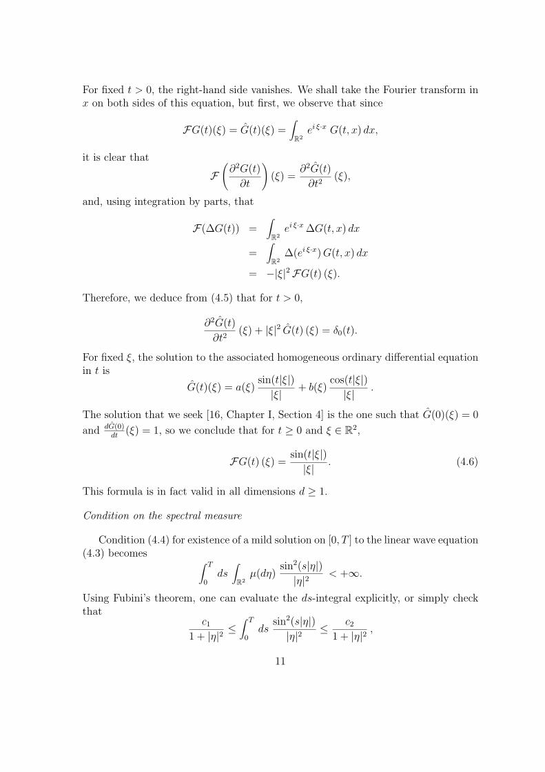
For fixed t > 0, the right-hand side vanishes. We shall take the Fourier transform inx on both sides of this equation, but first, we observe that since
FG(t)(ξ) = G(t)(ξ) =∫
R2ei ξ·x G(t, x) dx,
it is clear that
F(∂2G(t)
∂t
)(ξ) =
∂2G(t)
∂t2(ξ),
and, using integration by parts, that
F(∆G(t)) =∫
R2ei ξ·x ∆G(t, x) dx
=∫
R2∆(ei ξ·x)G(t, x) dx
= −|ξ|2FG(t) (ξ).
Therefore, we deduce from (4.5) that for t > 0,
∂2G(t)
∂t2(ξ) + |ξ|2 G(t) (ξ) = δ0(t).
For fixed ξ, the solution to the associated homogeneous ordinary differential equationin t is
G(t)(ξ) = a(ξ)sin(t|ξ|)|ξ|
+ b(ξ)cos(t|ξ|)|ξ|
.
The solution that we seek [16, Chapter I, Section 4] is the one such that G(0)(ξ) = 0
and dG(0)dt
(ξ) = 1, so we conclude that for t ≥ 0 and ξ ∈ R2,
FG(t) (ξ) =sin(t|ξ|)|ξ|
. (4.6)
This formula is in fact valid in all dimensions d ≥ 1.
Condition on the spectral measure
Condition (4.4) for existence of a mild solution on [0, T ] to the linear wave equation(4.3) becomes ∫ T
0ds∫
R2µ(dη)
sin2(s|η|)|η|2
< +∞.
Using Fubini’s theorem, one can evaluate the ds-integral explicitly, or simply checkthat
c11 + |η|2
≤∫ T
0ds
sin2(s|η|)|η|2
≤ c21 + |η|2
,
11
so condition (4.4) on the spectral measure becomes∫R2µ(dη)
1
1 + |η|2< +∞. (4.7)
Example 4.1 Consider the case where f(u) = |x|−β, 0 < β < d. In this case,µ(dη) = cd,β|η|β−d dy, so one checks immediately that condition (4.7) holds if andonly if β < 2. Therefore, the spatially homogeneous Gaussian noise is defined for0 < β < d, but a mild solution of the linear stochastic wave equation (4.3) exists ifand only if 0 < β < 2.
Reformulating (4.7) in terms of the covariance measure
Condition (4.7) on the spectral measure can be reformulated as a condition on thecovariance measure Γ. It is shown in [10] that in dimension d = 2, (4.7) is equivalentto ∫
|x|≤1Γ(dx) ln
(1
|x|
)< +∞,
while in dimensions d ≥ 3, (4.7) is equivalent to∫|x| ≤1
Γ(dx)1
|x|d−2< +∞.
In dimension d = 1, condition (4.7) is satisfied for any non-negative measure µ suchthat Γ = Fµ is also a non-negative measure.
The non-linear wave equation in dimension d = 2
We consider equation (4.1). The following theorem is the main result on existenceand uniqueness.
Theorem 4.2 Assume d = 2. Suppose that σ is a Lipschitz continuous function andthat condition (4.7) holds. Then there exists a unique solution (u(t, x), t ≥ 0, x ∈ R2)of (4.1) and for all p ≥ 1, this solution satisfies
sup0≤t≤T
supx∈Rd
E (|u(t, x)|p) <∞.
Proof. This proof follows a classical Picard iteration scheme. We set u0(t, x) = 0,and, by induction, for n ≥ 0,
un+1(t, x) =∫[0,t]×R2
G(t− s, x− y) σ(un(s, y)) M(ds, dy).
12

Before establishing convergence of this scheme, we first check that for p ≥ 2,
supn≥0
sup0≤s≤T
supx∈R2
E (|un(s, x)|p) < +∞.
We apply Burkholder’s inequality (2.3) and use the explicit form of the quadraticvariation of the stochastic integral [9, Theorem 5.26] to see that
E (|un+1(t, x)|p) ≤ cE(( ∫ t
0ds∫
R2dy
∫R2dz G(t− s, x− y) σ(un(s, y))
×f(y − z) G(t− s, x− z) σ(un(s, z))) p
2
).
Since G ≥ 0 and f ≥ 0, we apply Holder’s inequality in the form∣∣∣∣ ∫ f dµ
∣∣∣∣p ≤ (∫1 dµ
)p/q (∫|f |p dµ
), where
p
q= p− 1 (4.8)
and µ is a non-negative measure, to see that E (|un+1(t, x)|p) is bounded above by
c(∫ t
0ds∫
R2dy
∫R2dz G(t− s, x− y) f(y − z) G(t− s, x− z)
) p2−1
×∫ t
0ds∫
R2dy
∫R2dz G(t− s, x− y) f(y − z)G(t− s, x− z)
×E(|σ(un(s, y))σ(un(s, z))|
p2
).
We apply the Cauchy-Schwartz inequality to the expectation and use the Lipschitzproperty of σ to bound this by
C(∫ t
0ds∫
R2µ(dη) |FG(t− s)(η)|2
) p2−1
×∫ t
0ds∫
R2dy
∫R2dz G(t− s, x− y) f(y − z)G(t− s, x− z)
× (E (1 + |un(s, y)|p))1/2 (E (1 + |un(s, z)|p))1/2 .
Let
J(t) =∫ t
0ds∫
R2µ(dη) |FG(t− s)(η)|2 ≤ C
∫R2µ(dη)
1
1 + |η|2.
Then
E (|un+1(t, x)|p) ≤ C (J(t))p2−1∫ t
0ds
(1 + sup
y∈R2
E (|un(s, y)|p))
×∫
R2µ(dη) |FG(t− s)(η)|2
≤ C∫ t
0ds
(1 + sup
y∈R2
E(|un(s, y)|p)).
13
Therefore, if we setMn(t) = sup
x∈R2
E (|un(t, x)|p) ,
then
Mn+1(t) ≤ C∫ t
0ds (1 +Mn(s)) .
Using Gronwall’s lemma, we conclude that
supn∈N
sup0≤t≤T
Mn(t) < +∞.
We now check L2-convergence of the Picard iteration scheme. By the same rea-soning as above, we show that
supx∈R2
E (|un+1(t, x)− un(t, x)|p) ≤ C∫ t
0ds sup
y∈R2
E (|un(s, y)− un−1(s, y)|p) .
Gronwall’s lemma shows that (un(t, x), n ≥ 1) converges in L2(Ω, F , P ), uniformlyin x ∈ R2.
Uniqueness of the solution follows in a standard way: see [9, Proof of Theorem6.4]. 2
Holder-continuity (d = 2)
In order to establish Holder continuity of the solution to the stochastic waveequation in spatial dimension 2, we first recall the Kolmogorov continuity theorem. Itis a good idea to compare this statement with the equivalent one in [9, Theorem 4.3].
Theorem 4.3 (The Kolmogorov Continuity Theorem). Suppose that there is q > 0,ρ ∈ ]d
q, 1[ and C > 0 such that for all x, y ∈ Rd,
E (|u(t, x)− u(t, y)|q) ≤ C |x− y|ρq. (4.9)
Then x 7→ u(t, x) has a ρ-Holder continuous version, for any ρ ∈ ]0, ρ− dq[.
In order to use the statement of this theorem to establish (ρ−ε)-Holder continuity,for any ε > 0, it is necessary to obtain estimates on arbitrarily high moments ofincrements, that is, to establish (4.9) for arbitrarily large q.
Lq-moments of increments
From the integral equation (4.2), we see that
u(t, x)− u(s, y) =∫∫
(G(t− r, x− z)−G(s− r, y − z)) σ(u(r, z))M(dr, dz),
14
and so, by Burkholder’s inequality (2.3),
E (|u(t, x)− u(s, y)|p)
≤ C E
(∣∣∣∣∣∫ t
0dr∫
R2dz
∫R2dv (G(t− r, x− z)−G(s− r, y − z)) f(z − v)
× (G(t− r, x− v)−G(s− r, y − v))σ(u(r, z))σ(u(r, v))
∣∣∣∣∣p/2)
≤ C(∫
dr∫dz∫dv |G()−G()| f( ) |G()−G()|
) p2−1
×∫dr∫dz∫dv |G()−G()| f( ) |G()−G()|
×E(|σ(u(r, z))|p/2 |σ(u(r, v))|p/2
),
where the omitted variables are easily filled in. The Lipschitz property of σ implies abound of the type “linear growth”, and so, using also the Cauchy-Schwartz inequality,we see that the expectation is bounded by
C supr≤T, z∈R2
(1 + E(|u(r, z)|p)) .
Define
J(t, x ; s, y) =∫ t
0dr∫
R2dz∫
R2dv |G(t− r, x− z)−G(s− r, y − z)| f(z − v)
×|G(t− r, x− v)−G(s− r, y − v)|.
We have shown that
E (|u(t, x)− u(s, y)|p) ≤ (J(t, x ; s, y))p/2 .
Therefore, we will get Holder-continuity provided, for some γ > 0 and ρ > 0, we canestablish an estimate of the type
J(t, x ; s, y) ≤ c(|t− s|γ + |x− y|ρ).
Indeed, this will establish γ1
2-Holder continuity in time, and ρ1
2-Holder continuity in
in space, for all γ1 ∈ ]0, γ[ and ρ1 ∈ ]0, ρ[.
Analysis of J(t, x ; s, y)
If there were no absolute values around the increments of G, then we could use theFourier transform to rewrite J(t, x ; s, y), in the case x = y and s > t, for instance,as
J(t, x ; s, x) =∫ s
0dr∫
R2µ(dη) |FG(t− r)(η)−FG(s− r)(η)|2
+∫ t
sdr∫
R2µ(dη) |FG(t− r)(η)|2.
15
We could then analyse this using the specific form of FG in (4.6). However, thepresence of the absolute values makes this approach inoperable. By a direct analysisof J(t, x ; s, x), Sanz-Sole and Sarra [12] have established to following results. If∫
R2µ(dη)
1
(1 + |η|2)a<∞, for some a ∈ ]0, 1[,
then t 7→ u(t, x) is γ1-Holder continuous, for
γ1 ∈]0,
1
2∧ (1− a)
[,
and x 7→ u(t, x) is γ2-Holder continuous, for γ2 ∈ ]0, 1− a[.When µ(dη) = |η|−β dη, these intervals become
γ1 ∈]0,
1
2∧ 2− β
2
[and γ2 ∈
]0,
2− β
2
[.
We note that the best possible interval for γ1 is in fact ]0, 2−β2
[ (see [5, Chapter 5]).
5 A function-valued stochastic integral
Because the Green’s function in spatial dimension 3 is a measure and not a function,the study of the wave equation in this dimension requires different methods than thoseused in dimensions 1 and 2. In particular, we will use a function-valued stochasticintegral, developed in [4].
Our first objective is to define a stochastic integral of the form∫[0,t]×Rd
G(s, x− y) Z(s, y) M(ds, dy),
where G(s, ·) is the Green’s function of the wave equation (see Example 2.2) andZ(s, y) is a random field that plays the role of σ(u(s, y)).
We shall assume for the moment that d ≥ 1 and that the following conditions aresatisfied.
Hypotheses
(H1) For 0 ≤ s ≤ T, Z(s, ·) ∈ L2(Rd) a.s., Z(s, ·) is F s−measurable, and s 7→ Z(s, ·)from R+ → L2(Rd) is continuous.
(H2) For all s ≥ 0, ∫ T
0ds sup
ξ∈Rd
∫Rdµ(dη) |FG(s)(ξ − η)|2 < +∞.
16
We note that FG(s)(ξ − η) is given in (4.6), so that (H2) is a condition on thespectral measure µ, while (H1) is a condition on Z.
Fix ψ ∈ C∞0 (Rd) such that ψ ≥ 0, supp ψ ⊂ B(0, 1) and∫
Rdψ(x) dx = 1.
For n ≥ 1, setψn(x) = nd ψ(nx).
In particular, ψn → δ0 in S ′(Rd), and F ψn(ξ) = F ψ(ξ/n), so that |F ψn(ξ)| ≤ 1.Define
Gn(s, ·) = G(s) ∗ ψn,
so that Gn is a C∞0 -function. Then
vGn,Z(t, x)def=∫[0,t]×Rd
Gn(s, x− y) Z(s, y) M(ds, dy)
is well-defined as a Walsh-stochastic integral, and
E(‖vGn,Z(t, ·)‖2
L2(Rd)
)= IGn, Z , (5.1)
where
IGn,Z =∫
RddxE
((vGn,Z(t, x))2
)=
∫Rddx∫ t
0ds∫
Rddy∫
Rddz Gn(s, x− y)Z(s, y) f(y − z)
× Gn(s, x− z) Z(s, z).
Using the fact that the Fourier transform of a convolution (respectively product) isthe product (resp. convolution) of the Fourier transforms, one easily checks that
IGn,Z =∫ t
0ds∫
Rddξ E
(|FZ(s, ·)(ξ)|2
) ∫Rdµ(dη) |FGn(s, ·) (ξ − η)|2.
We note that:(a) the following inequality holds:
IGn,Z ≤ IGn,Z , (5.2)
where
IGn,Zdef=∫ t
0ds E
(‖Z(s, ·)‖2
L2(Rd)
)supξ∈Rd
∫Rdµ(dη) |FGn(s, ·)(ξ − η)|2; (5.3)
(b) the equality (5.1) plays the role of an isometry property;
17
(c) by elementary properties of convolution and Fourier transform,
IGn,Z ≤ IG,Z < +∞,
by (H2) and (H1).In addition, one checks that the stochastic integral
vG,Z(t)def= lim
n→∞vGn,Z
exists, in the sense that
E(‖vG,Z (t)− vGn,Z(t, ·)‖2
L2(Rd)
)−→ 0,
andE(‖vG,Z(t)‖2
L2(Rd)
)= IG,Z ≤ IG,Z .
We use the following notation for the stochastic integral that we have just defined:
vG,Z(t) =∫[0,t]×Rd
G(s, · − y) Z(s, y) M(ds, dy).
For t fixed, vG,Z(t) ∈ L2(Rd) is a square-integrable function that is defined almost-everywhere.
The definition of the stochastic integral requires in particular that hypothesis (H2)be satisfied. In the case where
Γ(dx) = kβ(x) dx, with kβ(x) = |x|−β, β > 0, (5.4)
this condition becomes∫ T
0ds sup
ξ∈Rd
∫Rddη |η|β−d sin2(s|ξ − η|)
|ξ − η|2< +∞.
One checks [4] that this is the case if and only if 0 < β < 2.
6 The wave equation in spatial dimension d ≥ 1
We consider the following stochastic wave equation in spatial dimension d ≥ 1, drivenby spatially homogeneous Gaussian noise F (t, x) as defined in Section 3:
(∂2u∂t2
−∆u)
(t, x) = σ(x, u(t, x)) F (t, x), t ∈ ]0, T ], x ∈ Rd,
u(0, x) = v0(x),∂u∂t
(0, x) = v0(x),
(6.1)
18
where v0 ∈ L2(Rd) and v0 ∈ H−1(Rd). By definition, H−1(Rd) is the set of square-integrable functions v0 such that
‖v0‖2H−1(Rd)
def=∫
Rddξ
1
1 + |ξ|2|F v0(ξ)|2 < +∞.
We shall restrict ourselves, though this is not really necessary (see [4]) to the casewhere Γ(dx) is as in (5.4), and 0 < β < 2.
The past-light cone property
Consider a bounded domain D ⊂ Rd. A fundamental property of the wave equa-tion is that u(T, x), x ∈ D, only depends on v0|KD and v0|KD , where
KD = y ∈ Rd : d(y,D) ≤ T
and d(y,D) denotes the distance from y to the set D, and on the noise F (s, y) fory ∈ KD(s), 0 ≤ s ≤ T , where
KD(s) =y ∈ Rd : d(y,D) ≤ T − s
.
Therefore, the solution u(t, x) in D is unchanged if we take the s.p.d.e.(∂2u
∂t2−∆u
)(t, x) = 1Kd(t)(x) σ(x, u(t, x)) F (t, x).
We shall make the following linear growth and Lipschitz continuity assumptionson the function σ.
Assumptions
(a) |σ(x, u)| ≤ c(1 + |u|) 1KD(x), for all x ∈ Rd and u ∈ R;
(b) |σ(x, u)− σ(x, v)| ≤ c |u− v|, for all x ∈ Rd and u, v ∈ R.
Definition 6.1 An adapted and mean-square continuous L2(Rd)-valued process (u(t), 0 ≤t ≤ T ) is a solution of (6.1) in D if for all t ∈ ]0, T ],
u(t) 1KD(t) = 1KD(t)
(d
dtG(t) ∗ v0 +G(t) ∗ v0
+∫[0,t]×Rd
G(t− s, · − y) σ(y, u(s, y)) M(ds, dy)
).
Theorem 6.2 Let d ≥ 1. Suppose 0 < β < 2 ∧ d and that the assumptions above onσ are satisfied. Then (6.1) has a unique solution (u(t), 0 ≤ t ≤ T ) in D.
19
Proof. We use a Picard iteration scheme. Set
u0(t, x) =d
dtG(t) ∗ v0 +G(t) ∗ v0.
We first check that u0(t) ∈ L2(Rd). Indeed,∥∥∥∥∥ ddt G(t) ∗ v0
∥∥∥∥∥L2(Rd)
=
∥∥∥∥∥F(d
dtG(t)
)· Fv0
∥∥∥∥∥L2(Rd)
=∫
Rddξ∣∣∣|ξ| cos(t|ξ|)
|ξ|· Fv0(ξ)
∣∣∣2≤ ‖v0‖L2(Rd) ,
and, similarly,‖G(t) ∗ v0‖L2(Rd) ≤ ‖v0‖H−1(Rd) .
One checks in a similar way that t 7→ u0(t) from [0, T ] into L2(Rd) is continuous.We now define the Picard iteration scheme. For n ≥ 0, assume that (un(t), 0 ≤
t ≤ T ) has been defined, and satisfies (H1). Set
un+1(t) = 1KD(t) (u0(t) + vn+1(t)) , (6.2)
wherevn+1(t) =
∫[0,t]×Rd
G(t− s, · − y) σ(y, un(s, y)) M(ds, dy). (6.3)
By induction, Zn(s, y) = σ(y, un(s, y)) satisfies (H1). Indeed, this process isadapted, and since
‖σ(·, un(s, ·))− σ(·, un(t, ·))‖L2(Rd) ≤ C‖un(s, ·)− un(t, ·)‖L2(Rd),
it follows that s 7→ un(s, ·) is mean-square continuous. One checks that un+1 alsosatisfies (H1): this uses assumption (a).
Therefore, the stochastic integral (6.3) is well-defined. Let
Mn(r) = sup0≤t≤r
E(‖un+1(t)− un(t)‖2
L2(KD(t))
)= sup
0≤t≤rE(‖vn+1(t)− vn(t)‖2
L2(KD(t))
)
= sup0≤t≤r
E
(∥∥∥∥ ∫[0,t]×Rd
G(t− s, · − y)
× (σ(y, un(s, y))− σ(y, un−1(s, y))) M(ds, dy)∥∥∥∥2
L2(KD(t))
)
≤ sup0≤t≤r
∫ t
0dsE
(‖σ(·, un(s, ·))− σ(·, un−1(s, ·))‖2
L2(KD(t))
)J(t− s),
20
where
J(s) = supξ∈Rd
∫Rddη |η|β−d sin2(s|ξ − η|)
|ξ − η|2.
A direct calculation shows that
sup0≤s≤T
J(s) < +∞,
since 0 < β < 2, so
Mn(r) ≤ C sup0≤t≤r
∫ t
0dsE
(‖un(s, ·)− un−1(s, ·)‖2
L2(KD(t))
),
that is,
Mn(r) ≤ C∫ r
0Mn−1(s) ds.
Because M0(T ) < +∞, Gronwall’s lemma implies that
+∞∑n=0
(Mn(r))1/2 < +∞.
Therefore, (un(t, ·), n ∈ N) converges in L2(Ω×Rd, dP × dx), uniformly in t ∈ [0, T ],to a limit u(t, ·). Since un satisfies (H1) and un converges uniformly in t to u(t, ·),it follows that u(t, ·) is a solution to (6.1): indeed, it suffices to pass to the limit in(6.2) and (6.3).
Uniqueness of the solution follows by a standard argument. 2
7 Spatial regularity of the stochastic integral (d =
3)
We aim now to analyze spatial regularity of the solution to the 3-dimensional stochas-tic wave equation (6.1) driven by spatially homogeneous Gaussian noise, with covari-ance given by a Riesz kernel f(x) = |x|−β, where 0 < β < 2. For this, we shall firstexamine the regularity in the x-variable of the function-valued stochastic integraldefined in Section 5 when d = 3.
We recall that studying regularity properties requires information on higher mo-ments. With these, one can use the Kolmogorov continuity theorem (Theorem 4.3)or the Sobolev embedding theorem, which we now recall.
Theorem 7.1 (The Sobolev Embedding Theorem). Suppose that g ∈ W p,q(O).Then x 7→ g(x) is ρ-Holder continuous, for all ρ ∈ ]0, ρ− d
q[ .
21
We recall [14] that the norm in the space W p,q(O) is defined by
‖g‖qW p,q(O) = ‖g‖q
Lq(O) + ‖g‖qp,q,O , (7.1)
where
‖g‖qLq(O) =
∫O|g(x)|q dx
‖g‖qp,q,O =
∫Odx
∫Ody
|g(x)− g(y)|q
|x− y|d+ρq.
Our first objective is to determine conditions that ensure that
E(‖vG,Z‖q
Lq(O)
)< +∞.
For ε > 0, we let
Oε =x ∈ R3 : ∃ z ∈ O with |x− z| < ε
denote the ε-enlargement of O, and use the notation
vtG,Z =
∫[0,t]×R3
G(t− s, · − y) Z(s, y) M(ds, dy).
An estimate in Lp-norm
Theorem 7.2 Suppose 0 < β < 2. Fix T > 0, q ∈ [2,+∞[ and let O ⊂ R3 be abounded domain. Suppose that∫ t
0ds E
(‖Z(s)‖q
Lq(Ot−s)
)< +∞.
Then
E(‖vt
G,Z‖qLq(O)
)≤ C
∫ t
0dsE
(‖Z(s)‖q
Lq(Ot−s)
).
Proof. We present the main ideas, omitting some technical issues that are handledin [5, Proposition 3.4]. First, we check inequality with G replaced by Gn :
E(‖vt
Gn,Z‖qLq(O)
)=∫OdxE
(∣∣∣ ∫[0,t]×R3
Gn(t− s, x− y) Z(s, y) M(ds, dy)∣∣∣q)
≤∫OdxE
(∣∣∣ ∫ t
0ds∫
R3dy∫
R3dz Gn (t− s, x− y) Z(s, y) f(y − z)
×Gn(t− s, x− z)Z(s, z)∣∣∣q/2
).
22
Let
µn(t, x) =∫ t
0ds∫
R3dy∫
R3dz Gn(t− s, x− y) f(y − z) Gn(t− s, x− z).
Assume thatsup
n, x, t≤Tµn(t, x) < +∞. (7.2)
By Holder’s inequality, written in the form (4.8), we see, since Gn ≥ 0, that
E(‖vt
Gn,Z‖qLq(O)
)≤
∫Odx (µn(t, x))
q2−1E
(∫ t
0ds∫
R3dy∫
R3dz Gn(t− s, x− y)
×f(y − z) Gn(t− s, x− z) |Z(s, y)|q/2 |Z(s, z)|q/2
)= I
Gn , |Z 1Ot−s+1/n|q/2 .
We apply (5.2), then (5.3), to bound this by
IGn , |Z 1Ot−s+1/n|q/2 =
∫ t
0dsE
(‖ |Z(s)|q/2 1Ot−s+1/n‖2
L2(R3)
)× sup
ξ∈R3
∫R3µ(dη) |FGn(s, ·)(ξ − η)|2.
Since 0 < β < 2, the supremum over ξ is finite, therefore
E(‖vt
Gn,Z‖qLq(O)
)≤ C
∫ t
0dsE
(‖Z(s)‖q
Lq(Ot−s+1/n)
).
By Fatou’s lemma,
E(‖vt
G,Z‖qLq(O)
)≤ lim inf
k→∞E(‖vt
Gnk,Z‖q
Lq(O)
)≤ lim inf
k→∞
∫ t
0dsE
(‖Z(s)‖q
Lq(Ot−s+1/nk )
)=
∫ t
0dsE
(‖Z(s)‖q
Lq(Ot−s)
).
It remains to check that (7.2) holds. Since
|FGn(t− s)(η)|2 ≤ |FG(t− s)(η)|2 =sin2((t− s)|η|)
|η|2,
it follows that for t ∈ [0, T ] and x ∈ R3,
µn(t, x) ≤∫ t
0ds∫
R3dη |η|β−3 sin2((t− s)|η|)
|η|2≤ C(T ),
23

since 0 < β < 2. This completes the proof. 2
An estimate in Sobolev norm
We consider here a spatially homogeneous Gaussian noise F (t, x), with covariancegiven by f(x) = |x|−β, where 0 < β < 2. We seek an estimate of the Sobolev normof the stochastic integral vt
G,Z . We recall that the Sobolev norm is defined in (7.1).
Theorem 7.3 Suppose 0 < β < 2. Fix T > 0, q ∈ ]3,+∞[, and let O ⊂ R3 be abounded domain. Fix γ ∈ ]0, 1[, and suppose that∫ t
0dsE
(‖Z(s)‖q
W γ,q(Ot−s)
)< +∞.
Consider
ρ ∈]0, γ ∧
(2− β
2− 3
q
) [.
Then there exists C < +∞ (depending on ρ but not on Z) such that
E(‖vt
G,Z‖qρ,q,O
)≤ C
∫ t
0dsE
(‖Z(s)‖q
W ρ,q(Ot−s)
).
Remark 7.4 In the case of the heat equation, spatial regularity of the stochasticintegral process, that is, of x 7→ vt
G,Z(x), occurs because of regularity of the heatkernel G, even if Z is merely integrable. Here, the spatial regularity of vt
G,Z is due tothe regularity of Z.
Proof of Theorem 7.3. The key quantity that we need to estimate is
E
(∫Odx
∫Ody|vt
G,Z(x)− vtG,Z(y)|q
|x− y|3+ρq
).
Let ρ = ρ+ 3q, so that 3+ρ q = ρ q. If we replace G by Gn, then the numerator above
is equal to∣∣∣∣ ∫ t
0ds∫
R3(Gn(t− s, x− u)−Gn(t− s, y − u)) Z(s, u) M(ds, du)
∣∣∣∣q,so by Burkholder’s inequality (2.3),
E(|vt
Gn,Z(x)− vtGn,Z(y)|q
)≤ C E
(∣∣∣∣ ∫ t
0ds∫
R3du∫
R3dv Z(s, u) f(u− v) Z(s, v) (7.3)
× (Gn(t− s, x− u)−Gn(t− s, y − u))
×(Gn(t− s, x− v)−Gn(t− s, y − v))∣∣∣∣q/2)
.
24
If we had G instead of Gn, and if G were smooth, then we would get a bound involvingan exponent of |x− y|, even if Z were merely integrable.
Here we use a different idea: we shall pass the increments on the Gn over to thefactors Z f Z by changing variables. For instance, if there were only one factor involv-ing increments of Gn, we could use the following calculation, where Gn is genericallydenoted g and Z f Z is denoted ψ:∫
R3du (g(x− u)− g(y − u))ψ(u)
=∫
R3du g(x− u)ψ(u)−
∫R3du g(y − u)ψ(u)
=∫
R3du g(u)ψ(x− u)−
∫R3du g(u)ψ(y − u)
)
=∫
R3du g(u) (ψ(x− u)− ψ(y − u)).
Using this idea, it turns out that the integral on the right-hand side of (7.3) is equalto
4∑i=1
J ti,n (x, y),
where
J ti,n(x, y) =
∫ t
0ds∫
R3du∫
R3dv Gn(s, u) Gn(s, v) hi(t, s, x, y, u, v),
and
h1(t, s, x, y, u, v) = f(y − x+ v − u) (Z(t− s, x− u)− Z(t− s, y − u))×(Z(t− s, x− v)− Z(t− s, y − v),
h2(t, s, x, y, u, v) = Df(v − u, x− y)Z(t− s, x− u)×(Z(t− s, x− v)− Z(t− s, y − v)),
h3(t, s, x, y, u, v) = Df(v − u, y − x)Z(t− s, y − v)×(Z(t− s, x− u)− Z(t− s, y − u)),
h4(t, s, x, y, u, v) = −D2f (v − u, x− y) Z(t− s, x− u) Z(t− s, x− u),
and we use the notation
Df(u, x) = f(u+ x)− f(u),
D2f(u, x) = f(u− x)− 2 f(u) + f(u+ x).
We can now estimate separately each of the four terms
T in(t,O) =
∫Odx∫Ody
E(|J ti,n(x, y)|q/2)
|x− y|ρ q, i = 1, . . . , 4.
25
The term T 1n(t,O). Set
µn(x, y) = sups∈[0,T ]
∫R3du∫
R3dv Gn(s, u) Gn(s, v) f(y − x+ v − u)
= sups∈[0,T ]
∫R3µ(dη) ei η·(x−y)|FGn(s)(η)|2,
so thatsupn,x,y
µn(x, y) < +∞
since β < 2. Therefore, since Gn(s, u) ≥ 0, by Holder’s inequality,
E(|J t
1,n(x, y)|q/2)
≤ (T µn(x, y))q2−1
×E(∫ t
0ds∫
R3du∫
R3dv Gn(s, u) Gn(s, v) f(y − x+ v − u)
×|Z(t− s, x− u)− Z(t− s, y − u)|q/2
×|Z(t− s, x− v)− Z(t− s, y − v)|q/2
).
Apply the Cauchy-Schwarz inequality with respect to the measure
dP dx dy ds du dv Gn(s, u)Gn(s, v) f(y − x+ v − u)
to see that
T 1n(t,O) ≤
(T 1,1
n (t,O) T 1,2n (t,O)
)1/2,
where
T 1,1n (t,O) =
∫ t
0ds∫Odx∫Ody∫
R3du∫
R3dv Gn(s, u) Gn(s, v) f(y − x+ v − u)
×E (|Z(t− s, x− u)− Z(t− s, y − u)|q)|x− y|ρq
,
and there is an analogous expression for T 1,2n (t,O). We note that for x ∈ O, when
Gn(s, u) > 0 (resp. for y ∈ O, when Gn(s, v) > 0), x − u ∈ Os(1+1/n) (resp. y − u ∈Os(1+1/n)), so
T 1,1n (t,O) ≤
∫ t
0dsE
(‖Z(t− s)‖q
ρ,q,Os(1+1/n)
)supn,x,y
µn(x, y).
The same bound arises for the term T 1,2n (t,O), so this gives the desired estimate for
this term.We shall not discuss the terms T 2
n(t,O) and T 3n(t,O) here: the interested reader
may consult [5, Chapter 3], but we consider the term T 4n(t,O).
26
The term T 4n(t,O). In order to bound T 4
n(t,O), we aim to bring the exponent q/2inside the ds du dv integral, in such a way that it only affects the Z factors but not f .
Set
µn(x, y) = sups∈[0,T ]
∫R3du∫
R3dv Gn(s, u) Gn(s, v)
|D2f(v − u, x− y)||x− y|2ρ
. (7.4)
We will show below that
supn≥1, x,y∈O
µn(x, y) ≤ C < +∞, (7.5)
which will turn out to require quite an interesting calculation. Assuming this for themoment, let p = q/2. Then, by Holder’s inequality,
E(|J t
4,n(x, y)|p)
|x− y|2pρ
≤ supn,x,y
(µn(x, y))p−1∫ t
0ds∫
R3du∫
R3dv Gn(s, u) Gn(s, v)
× |D2f(v − u, x− y)||x− y|2ρ
E (|Z(t− s, x− u)|p |Z(t− s, x− v)|p) .
This quantity must be integrated over O×O. We apply the Cauchy-Schwarz inequal-ity to the measure ds du dv(· · · )dP , and this leads to
T 4n(t,O) ≤ sup
n,x,y(µn(x, y))p
∫ t
0dsE
(‖Z(s)‖q
Lq(O(t−s)(1+1/n))
).
This is the desired bound for this term.It remains to check (7.5). The main difficulty is to bound the second order differ-
ence |D2f(v − u, x− y)|. We explain the main issues below.
Bounding symmetric differences
Let g : R → R. Suppose that we seek a bound on
D2g(x, h) = g(x− h)− 2g(x) + g(x+ h).
Notice that if g is differentiable only once (g ∈ C1), then the best that we can do isessentially to write
|D2g(x, h)| ≤ |g(x− h)− g(x)|+ |g(x+ h)− g(x)|≤ c h.
On the other hand, if g is twice differentiable (g ∈ C2), then we can do better:
|D2g(x, h)| ≤ c h2.
27
In the case of a Riesz kernel f(x) = |x|−β, x ∈ R3, we can write
|D2f(u, x)| =∣∣∣ |u− x|−β − 2|u|−β + |u+ x|−β
∣∣∣≤ C |f ′′(u)| |x|2
= C |u|−β−2 |x|2 .
Taking into account the definition of µn(x, y) in (7.4), this inequality leads to thebound
µn(x, y) ≤ sups∈[0,T ]
(∫R3du∫
R3dv Gn(s, u) Gn(s, v) |u− v|−(β+2)
) |x− y|2
|x− y|2ρ.
However, the double integral converges to +∞ as n→∞, since β + 2 > 2.Since differentiating once does not necessarily give the best bound possible and
differentiating twice gives a better exponent but with an infinite constant, it is naturalto want to differentiate a fractional number of times, namely just under 2− β times.If we “differentiate α times” and all goes well, then this should give a bound of theform µn(x, y) ≤ C|x− y|α, for α ∈ ]0, 2− β[. We shall make this precise below.
Riesz potentials, their fractional integrals and Laplacians
Let αdef= 2ρ. We recall that
ρ <2− β
2− 3
qand ρ = ρ+
3
q, so α < 2− β.
The Riesz potential of a function ϕ : Rd → R is defined by
(Ia ϕ)(x) =1
γ(a)
∫Rd
ϕ(y)
|x− y|d−ady, a ∈ ]0, d[,
where γ(a) = πd/22aΓ(a/2)/Γ(d−a2
). Riesz potentials have many interesting properties(see [15]), of which we mention the following.
(1) Ia+b(ϕ) = Ia(Ib ϕ) if a + b ∈ ]0, d[. Further, Ia can be seen as a “fractionalintegral of order a”, in the sense that
F(Ia ϕ)(ξ) = Fϕ(ξ)F(
1
| · |d−a
)(ξ) =
Fϕ(ξ)
|ξ|a.
(2) Our covariance function kβ(x) = |x|−β is a Riesz kernel. These kernels havethe following property:
|x|−d+a+b =∫
Rddz kd−b(x− z) |z|−d+a (7.6)
= Ib(| · |−d+a
). (7.7)
28
This equality can be viewed as saying that |z|−d+a is “bth derivative (or Laplacian)”of |z|−d+a+b, in the sense that
(−∆)b/2(|z|−d+a+b
)= |z|−d+a .
Indeed, taking Fourier transforms, this equality becomes simply
|ξ|b |ξ|−a−b = |ξ|−a .
Recall the notationDf(u, y) = f(u+ y)− f(u).
From (7.6), one can easily deduce (see [5, Lemma 2.6]) that
Dkd−a−b(u, cx) = |c|b∫
Rddw kd−a(u− cw) Dkd−b(w, x)
and
|D2kd−a−b(u, x)| ≤ |x|b∫
Rddw kd−a(u− |x|w) D2kd−b
(w,
x
‖x‖
).
Set b = α = 2ρ and a = 3 − α − β, where α + β ∈ ]0, 2[ . Looking back to (7.4),these two relations lead to the following estimate:
µn(x, y) ≤ sups∈ [0,T ]
1
|x− y|α∫
R3du∫
R3dv Gn(s, u) Gn(s, v) |x− y|α
×∫
R3dw kα+β(v − u− |y − x|w)×
∣∣∣D2k3−α
(w,
x
|x|
) ∣∣∣≤ sup
s∈ [0,T ]
(supx,y,w
∫R3du∫
R3dv Gn(s, u) Gn(s, v) kα+β(v − u− |y − x|w)
)
× supx
∫dw
∣∣∣D2k3−α
(w,
x
‖x‖
) ∣∣∣ .The double integral above is finite since α+β < 2. Indeed, taking Fourier transforms,the shift −|y − x|w introduces a factor eiη·|y−x|w, which is of no consequence. Thesecond integral is finite (and does not depend on x). For this calculation, see [5,Lemma 2.6]. 2
8 Holder-continuity in the 3-d wave equation
We consider the stochastic wave equation (6.1) for d = 3, driven by spatially homo-geneous Gaussian noise with covariance f(x) = |x|−β, where 0 < β < 2.
The main idea for checking Holder continuity of the solution is to go back tothe Picard iteration scheme that was used to construct the solution, starting with
29
a smooth function u0(t, x) (whose smoothness depends only on the regularity of theinitial conditions), and then check that regularity is preserved at each iteration stepand passes to the limit. The details are carried out in [5, Chapter 4]. The main resultis the following.
Theorem 8.1 Assume the following three properties:
(a) the initial value v0 is such that v0 ∈ C2(R3) and ∆v0 is Holder continuous withexponent γ1;
(b) the initial velocity v0 is Holder continuous with exponent γ2;
(c) the nonlinearities σ, b : R → R are Lipschitz continuous.
Then, for any q ∈ [2,∞[ and
α ∈ ]0, γ1 ∧ γ2 ∧2− β
2[ , (8.1)
there is C > 0 such that for all (t, x), (s, y) ∈ [0, T ]×D,
E (|u(t, x)− u(s, y)|q) ≤ C (|t− s|+ |x− y|)αq .
In particular, (t, x) 7→ u(t, x) has a Holder continuous version with exponent α.
We observe that the presence of γ1 ∧ γ2 in (8.1) can be interpreted by saying thatthe (ir)regularity of the initial conditions limits the possible regularity of the solution:there is no smoothing effect in the wave equation, contrary to the heat equation.
We note that this result is sharp. Indeed, if we consider the linear wave equation,in which we take σ ≡ 1 and b ≡ 0 in (6.1), with vanishing initial condition v0 ≡ v0 ≡ 0,then it is possible to show (see [5, Chapter 5] that
E(|u(t, x)− u(t, y)|2
)≥ c1 |x− y|2−β
andE(|u(t, x)− u(s, x)|2
)≥ c2 |t− s|2−β.
This implies in particular that t 7→ u(t, x) and x 7→ u(t, x) are not γ-Holder continu-ous, for γ > 2−β
2.
References
[1] R.C. Dalang: Extending the martingale measure stochastic integral with applica-tions to spatially homogeneous spde’s. Electronic J. of Probability, Vol 4, 1999.
30
[2] R.C. Dalang, N.E. Frangos: The stochastic wave equation in two spatial dimen-sions. Annals of Probab. 26, 1, 187-212, 1998.
[3] R.C. Dalang, O. Leveque: Second-order linear hyperbolic SPDEs driven byisotropic Gaussian noise on a sphere. Annals of Probab. 32, 1068–1099, 2004.
[4] R.C. Dalang, C. Mueller: Some non-linear SPDE’s that are second order in time.Electronic J. of Probability, Vol 8, 1, 1-21, 2003.
[5] R.C. Dalang, M. Sanz-Sole: Holder-Sobolev regularity of the solution to thestochastic wave equation in dimension 3. Memoirs of the AMS (2007, to appear).
[6] G.B. Folland: Introduction to Partial Differential Equations. Princeton Univ.Press, 1976.
[7] O. Gonzalez, J.H. Maddocks: Extracting parameters for base-pair level modelsof DNA from molecular dynamics simulations. Theoretical Chemistry Accounts,106, 76-82, 2001.
[8] A. Hellemans: SOHO Probes Sun’s Interior by Tuning In to Its Vibrations. Sci-ence May 31 1996: 1264-1265.
[9] D. Khoshnevisan: A Primer on Stochastic Partial Differential Equations. In:this volume, 2007.
[10] A. Karkzewska, J. Zabczyk: Stochastic PDE’s with function-valued solutions.In: Infinite-dimensional stochastic analysis (Clement Ph., den Hollander F., vanNeerven J. & de Pagter B., eds), pp. 197-216, Proceedings of the Colloquium ofthe Royal Netherlands Academy of Arts and Sciences, 1999, Amsterdam.
[11] M. Oberguggenberger & F. Russo: Nonlinear stochastic wave equations. In:Generalized functions—linear and nonlinear problems (Novi Sad, 1996). Inte-gral Transform. Spec. Funct. 6, no. 1-4, 71–83, 1998.
[12] M. Sanz-Sole, M. Sarra: Holder continuity for the stochastic heat equation withspatially correlated noise. In: Stochastic analysis, random fields and applications(R.C. Dalang, M. Dozzi & F. Russo, eds), pp. 259-268, Progress in Probability52, Birkhauser, Basel, 2002.
[13] L. Schwartz: Theorie des distributions. Hermann, Paris, 1966.
[14] N. Shimakura: Partial differential operators of elliptic type. Translations ofMathematical Monographs, 99. American Mathematical Society, 1992.
[15] E. M. Stein: Singular Integrals and Differentiability Properties of Functions.Princeton University Press, Princeton, 1970.
31
[16] F. Treves: Basic Linear Partial Differential Equations. Academic Press, 1975.
[17] J.B. Walsh: An introduction to stochastic partial differential equations, Ecoled’ete de Probabilites de Saint Flour XIV, Lecture Notes in Mathematics, Vol.1180, Springer Verlag, 1986.
[18] J. Zabczyk: A mini course on stochastic partial differential equations. In:Stochastic climate models (P. Imkeller & J.-S. von Storch, eds), pp. 257–284,Progr. Probab., 49, Birkhuser, 2001.
32