Embed Size (px)
Citation preview

Some aspects of seismic design methods for flexible earth retaining structures
Quelques aspects des méthodes du projet séismiques pour les structures de retenue de la terre flexible
Ciro Visone
DIG, University of Naples Federico II, Naples, Italy [email protected]
Filippo Santucci de Magistris SAVA, Engineering & Environmental Div., University of Molise, Campobasso, Italy [email protected]
ABSTRACT
On the basis of Performance-based design philosophy and hierarchical resistances, in this paper some consid-erations are done for flexible earth retaining structures. Structural damage and serviceability criteria adopted in existing codes and guidelines are illustrated. A series of results of numerical analyses conducted with a FE code and the influence of some parameters on the results of dynamic analysis are discussed. A new pseu-dostatic approach and its application procedure are proposed.
RÉSUMÉ
Sur la base de la philosophie de conception Performance-basée et des résistances hiérarchiques, en cet article quelques considérations sont faites pour les structures de retenue de la terre flexible. Des critères structuraux de dommages et d'utilité adoptés dans des codes existants et des directives sont analysés. Une série de résultats des analyses numériques conduites avec un code de Fe et l'influence de quelques paramètres sur les résultats de l'analyse dynamique est discutée. On propose une nouvelle approche pseudostatic et son procédé d'application.
Keywords: flexible retaining walls, hierarchical resistance, push-over analyses
1 INTRODUCTION.
The seismic design of flexible retaining walls is often conducted using limit equilibrium methods and calculating the dynamic earth pressures with the Mononobe & Okabe M-O theory. This type of analysis does not permit the evaluation of system re-sponse in terms of displacements. An alternative method is the use of subgrade reaction analyses, in which the soil is idealized as a series of elasto-plastic springs characterized by means of coeffi-cients of subgrade reaction, and the structural ele-ment is modelled as an elastic or elasto-plastic beam. This approach allows the calculation of the elastic and plastic deformations induced in the soil but the values of displacements are realistic only if the stress and strain relationships of the springs are cho-sen with a great accuracy.
For the response of flexible earth retaining struc-ture under seismic loadings, both methods cannot take into account of some aspects that might influ-ence the overall behaviour of the system i.e., the damping, the natural frequencies of the system, the phase differences and the amplification effects within the backfill. Using a simple pseudodynamic analysis of seismic earth pressures, Steedman &
Zeng (1990) have shown that the earth pressure dis-tribution and the point of application of the dynamic thrust are ruled by the frequency motions, as well as the properties of backfill.
Therefore, it seems that new calculation ap-proaches are needed in order to consider the influ-ence of these aspects even in a simplified manner. Also, it would be helpful that the calculation meth-ods eventually indicate the parameters for specifying damage criteria, in terms of displacements and stresses. All these aspects are neglected also in mod-ern seismic codes, including Eurocode 8 and the de-rived Italian code OPCM3274, 2003.
For most relevant structures, some codes and guidelines suggest the use of dynamic analyses. Numerous parameters might affect the results of the latter. Also, their proper use is often confined in re-search environment, since they required a skill level that is often not common among practitioners.
To shade some light on the points listed above, in this paper some aspects related to the calibration of a numerical model that should be conducted before performing a dynamic analysis are discussed. For an ideal RC diaphragm embedded in a uniform granular soil layer, some complete dynamic analyses were carried out.

Also, in order to simplify the seismic design of flexible retaining walls, a new approach is presented that allow knowing the behaviour of soil-structure system till the collapse. The application of the method to the given case is illustrated.
2 EARTHQUAKE PROVISIONS DESCRIBED IN SOME EXISTING CODES AND GUIDELINES.
Eurocode 8 part 5 (EN 1998-5, 2003) states that earth retaining structures must design to fulfil their function during and after an earthquake, without suf-fering significant structural damages. Permanent displacements, in the form of combined sliding and tilting, the latter due to irreversible deformations of the foundation soil, may be acceptable if it is shown that they are compatible with functional and/or aes-thetic requirements. In the same document is indi-cated that any established method based on the pro-cedures of structural and soil dynamics, and supported by experience and observations, is in principle acceptable for assessing the safety of an earth-retaining structure. The aspects needed con-sider are:
a) the generally non-linear behaviour of the soil in the course of its dynamic interaction with the retaining structure;
b) the inertial effects associated with the masses of the soil, of the structure, and of all other gravity loads which might participate in the interaction process;
c) the hydrodynamic effects generated by the presence of water in the soil behind the wall and/or by the water on the outer face of the wall;
d) the compatibility between the deformations of the soil, the wall, and the tiebacks, when present.
It should be underlined that no indications on rep-resentative parameters for specifying damage criteria and no limitations on values of the displacements are given.
The basic components that should be included in a pseudo-static analysis consist in the retaining structure and its foundation, in a soil wedge behind the structure supposed to be in a state of active limit equilibrium (if the structure is flexible enough), in any surcharge loading acting on the soil wedge, and, possibly, in a soil mass at the foot of the wall, sup-posed to be in a state of passive equilibrium.
In EC8 part 5, the possible movements of the sys-tem are accounted only with the r factor that is in-cluded into determination of seismic coefficients. Dynamic earth pressures are calculated with M-O theory and the wall friction angle must to be taken not higher than δ=2/3φ, for active state, in which φ
is the angle of shear resistance of soil, and δ=0, for passive state.
As previously underlined, this approach suffers of some limitations. Deformability of structure, soil stiffness and damping, natural frequencies of system are neglected. The displacements of the wall and the backfill cannot provide.
Also Callisto (2006) highlighted some of the lim-its in the pseudostatic approach as indicated in EC8-5 and specified some preliminary correction to the code statements.
In PIANC (2001) the parameters for identifying damage criteria, in terms of displacements and stresses, for sheet pile quay wall (Figure 1) and pre-ferred sequence of yield of the system (Figure 2) can be found.
a)
Settelement of Apron
Differential Settlement of ApronTilting
Differential Settlement at Anchor
Ground Surface Cracking at Anchor
Pull-out Displacement of Battered Pile Anchor
Horizontal DisplacementSettlement
Differential Displacement
b)
Stress in Tie-rod
(including joints)
Stress in Anchor PileStress in Sheet Pile
(above and below mudline)
Figure 1. Parameters for specifying damage criteria: a) respect to displacements; b) respect to stresses (PIANC, 2001).
1) Displacement of Anchor
4) Yield at Anchor5) Yield at Tie-rod2) Yield at Sheet Pile Wall
(above mudline)
3) Yield at Sheet Pile Wall
(below mudline)
Figure 2. Preferred sequence of damages for sheet pile quay wall (PIANC, 2001).
It could be noted that the yield of soil for passive
state is not considered in the sequence and maybe might be included in the list. However, different and unclear opinions on this point exist in scientific community.
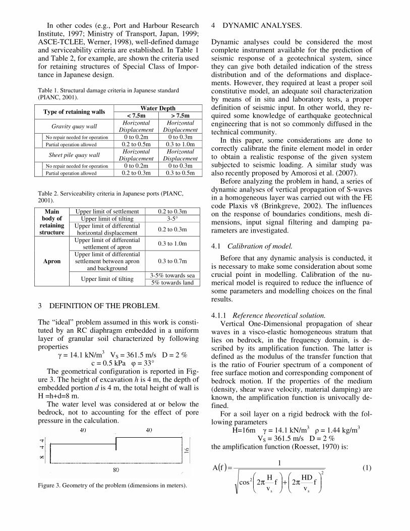
In other codes (e.g., Port and Harbour Research Institute, 1997; Ministry of Transport, Japan, 1999; ASCE-TCLEE, Werner, 1998), well-defined damage and serviceability criteria are established. In Table 1 and Table 2, for example, are shown the criteria used for retaining structures of Special Class of Impor-tance in Japanese design.
Table 1. Structural damage criteria in Japanese standard (PIANC, 2001).
Water Depth Type of retaining walls
< 7.5m > 7.5m
Gravity quay wall Horizontal
Displacement Horizontal
Displacement
No repair needed for operation 0 to 0.2m 0 to 0.3m Partial operation allowed 0.2 to 0.5m 0.3 to 1.0m
Sheet pile quay wall Horizontal
Displacement
Horizontal
Displacement
No repair needed for operation 0 to 0.2m 0 to 0.3m Partial operation allowed 0.2 to 0.3m 0.3 to 0.5m
Table 2. Serviceability criteria in Japanese ports (PIANC, 2001).
Upper limit of settlement 0.2 to 0.3m Upper limit of tilting 3-5°
Main body of
retaining structure
Upper limit of differential horizontal displacement 0.2 to 0.3m
Upper limit of differential settlement of apron 0.3 to 1.0m
Upper limit of differential settlement between apron
and background 0.3 to 0.7m
3-5% towards sea
Apron
Upper limit of tilting 5% towards land
3 DEFINITION OF THE PROBLEM.
The “ideal” problem assumed in this work is consti-tuted by an RC diaphragm embedded in a uniform layer of granular soil characterized by following properties
γ = 14.1 kN/m3 VS = 361.5 m/s D = 2 % c = 0.5 kPa φ = 33°
The geometrical configuration is reported in Fig-ure 3. The height of excavation h is 4 m, the depth of embedded portion d is 4 m, the total height of wall is H =h+d=8 m.
The water level was considered at or below the bedrock, not to accounting for the effect of pore pressure in the calculation.
Figure 3. Geometry of the problem (dimensions in meters).
4 DYNAMIC ANALYSES.
Dynamic analyses could be considered the most complete instrument available for the prediction of seismic response of a geotechnical system, since they can give both detailed indication of the stress distribution and of the deformations and displace-ments. However, they required at least a proper soil constitutive model, an adequate soil characterization by means of in situ and laboratory tests, a proper definition of seismic input. In other world, they re-quired some knowledge of earthquake geotechnical engineering that is not so commonly diffused in the technical community.
In this paper, some considerations are done to correctly calibrate the finite element model in order to obtain a realistic response of the given system subjected to seismic loading. A similar study was also recently proposed by Amorosi et al. (2007).
Before analyzing the problem in hand, a series of dynamic analyses of vertical propagation of S-waves in a homogeneous layer was carried out with the FE code Plaxis v8 (Brinkgreve, 2002). The influences on the response of boundaries conditions, mesh di-mensions, input signal filtering and damping pa-rameters are investigated.
4.1 Calibration of model.
Before that any dynamic analysis is conducted, it is necessary to make some consideration about some crucial point in modelling. Calibration of the nu-merical model is required to reduce the influence of some parameters and modelling choices on the final results.
4.1.1 Reference theoretical solution. Vertical One-Dimensional propagation of shear
waves in a visco-elastic homogeneous stratum that lies on bedrock, in the frequency domain, is de-scribed by its amplification function. The latter is defined as the modulus of the transfer function that is the ratio of Fourier spectrum of a component of free surface motion and corresponding component of bedrock motion. If the properties of the medium (density, shear wave velocity, material damping) are known, the amplification function is univocally de-fined.
For a soil layer on a rigid bedrock with the fol-lowing parameters
H=16m γ = 14.1 kN/m3 ρ = 1.44 kg/m3 VS = 361.5 m/s D = 2 %
the amplification function (Roesset, 1970) is:
( )2
ss
2 fv
HD2f
v
H2cos
1fA
π+
π
= (1)

Figure 4 shows its graphical representation. Here, and in the following similar figures, two vertical red lines indicate the first and the second natural fre-quency of the system.
0
5
10
15
20
25
30
0 5 10 15 20 25
Frequency Hz
Am
pli
fic
ati
on
rati
o
1st natural frequency
f1=5.65 Hz
2nd
natural frequency
f2=16.95 Hz
Figure 4. Amplification function of an elastic medium over rigid bedrock.
4.1.2 Input signal and finite element model. Input signal chosen for numerical analyses is the
accelerometer registration of Tolmezzo Station (Friuli Earthquake, Italy, May 6th, 1976). The sam-pling frequency is 200 Hz, the duration is 36.39 sec and the peak acceleration is 0.315 g. Three other dif-ferent inputs are used in analysis, scaling this signal down to a PGA=1 cm/sec2, a PGA= 0.05 g and a PGA=0.1 g.
Accelerations time-history and Fourier Spectrum of the signal are reported in Figure 5.
a)
-0.4
-0.3
-0.2
-0.1
0
0.1
0.2
0.3
0.4
0 5 10 15 20 25 30 35
Time (sec)
Ac
cele
rati
on
(g
)
b)
0
0.05
0.1
0.15
0.2
0.25
0 5 10 15 20 25
Frequency Hz
Fo
uri
er
Am
plitu
de
Figure 5. Seismic input: a) accelerations time-history; b) Fou-rier Spectrum.
In numerical computation, the earthquake loading was imposed as an acceleration time-history at the base of the model.
The finite element model is plotted in Figure 5. It is constituted by a rectangular domain 80 m wide and 16 m high and two similar lateral domains in or-der to place far enough the lateral boundaries (total width 240 m). This model was calibrated to mini-mize the influence of the boundaries on the obtained results. The soil is schematized with a Mohr-Coulomb M-C model that is implemented in the code Plaxis. Its parameters are indicated in Table 3.
Figure 5. Finite element model utilized in the dynamic analy-ses. Table 3. General information and material properties of the M-C model.
GENERAL INFORMATIONS
Material model Water Level
Mohr-Coulomb Absent PHYSICAL PROPERTIES
RAYLEIGH DAMPING γ [kN/m
3] e0 α β
14.1 0.844 - - STIFFNESS PARAMETERS
E [kN/m2] 4.889x10⁵ Eoed [kN/m
2] 6.581x10⁵
υ 0.3 vs [m/s] 361.5 G [kN/m
2] 1.88x10⁵ vp [m/s] 676.3
STRENGTH PARAMETERS
c [kPa] φ [°] ψ [°] Rinter
0.5 33 0 0.622
The initial stress generation was executed by the k0-procedure in which the value of k0 was chosen by means of the well-known Jaky’s formula.
455.0sin1k 0 =ϕ−= (2)
The diaphragm is idealized using an elastic plate element with the properties summarized in Table 4.
Table 4. Elastic properties of RC Diaphragm.
ELASTIC PLATE
EA [kN/m] EI [kNm2/m] w [kN/m
3/m] ν
32000000 2666667 10.9 0.3
Soil-structure friction is simulated with an inter-face element characterized by Rinter parameter im-posed equal to
622.0tan
tanR erint =
ϕ
δ= (3)
that corresponds to assume a soil-wall friction angle δ=2/3φ=22°.
The mesh generation in Plaxis is fully automatic and based on a robust triangulation procedure, which
80m 80m 80m
results in an “unstructured” mesh. In the meshes used in the present analyses, the basic type of ele-ment is the 15-node triangular element. The size of any element can be controlled by local element size. Subdividing the homogeneous layer in sub-layers with a fixed thickness and using the local element size, it is possible to decide the maximum dimension of cathetus of triangles in which is discretized the domain.
An average dimension that is representative for refinement degree of the mesh is the “Average Ele-ment Size” (AES) that represents an average length of the side of the elements employed.
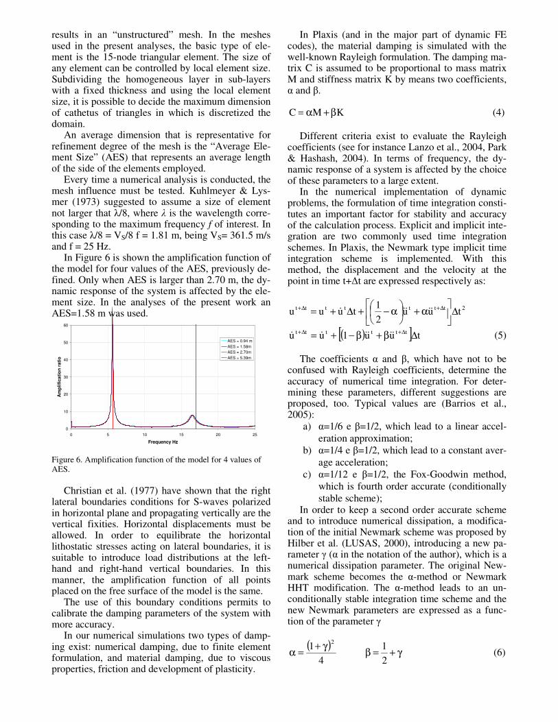
Every time a numerical analysis is conducted, the mesh influence must be tested. Kuhlmeyer & Lys-mer (1973) suggested to assume a size of element not larger that λ/8, where λ is the wavelength corre-sponding to the maximum frequency f of interest. In this case λ/8 = VS/8 f = 1.81 m, being VS= 361.5 m/s and f = 25 Hz.
In Figure 6 is shown the amplification function of the model for four values of the AES, previously de-fined. Only when AES is larger than 2.70 m, the dy-namic response of the system is affected by the ele-ment size. In the analyses of the present work an AES=1.58 m was used.
0
10
20
30
40
50
60
0 5 10 15 20 25
Frequency Hz
Am
pli
fica
tio
n r
ati
o
AES = 0.94 m
AES = 1.58m
AES = 2.70m
AES = 5.39m
Figure 6. Amplification function of the model for 4 values of AES.
Christian et al. (1977) have shown that the right
lateral boundaries conditions for S-waves polarized in horizontal plane and propagating vertically are the vertical fixities. Horizontal displacements must be allowed. In order to equilibrate the horizontal lithostatic stresses acting on lateral boundaries, it is suitable to introduce load distributions at the left-hand and right-hand vertical boundaries. In this manner, the amplification function of all points placed on the free surface of the model is the same.
The use of this boundary conditions permits to calibrate the damping parameters of the system with more accuracy.
In our numerical simulations two types of damp-ing exist: numerical damping, due to finite element formulation, and material damping, due to viscous properties, friction and development of plasticity.
In Plaxis (and in the major part of dynamic FE codes), the material damping is simulated with the well-known Rayleigh formulation. The damping ma-trix C is assumed to be proportional to mass matrix M and stiffness matrix K by means two coefficients, α and β.
KMC β+α= (4)
Different criteria exist to evaluate the Rayleigh coefficients (see for instance Lanzo et al., 2004, Park & Hashash, 2004). In terms of frequency, the dy-namic response of a system is affected by the choice of these parameters to a large extent.
In the numerical implementation of dynamic problems, the formulation of time integration consti-tutes an important factor for stability and accuracy of the calculation process. Explicit and implicit inte-gration are two commonly used time integration schemes. In Plaxis, the Newmark type implicit time integration scheme is implemented. With this method, the displacement and the velocity at the point in time t+∆t are expressed respectively as:
2ttttttt tuu2
1tuuu ∆
α+
α−+∆+= ∆+∆+
&&&&&
( )[ ] tuu1uu tttttt ∆β+β−+= ∆+∆+&&&&&& (5)
The coefficients α and β, which have not to be confused with Rayleigh coefficients, determine the accuracy of numerical time integration. For deter-mining these parameters, different suggestions are proposed, too. Typical values are (Barrios et al., 2005):
a) α=1/6 e β=1/2, which lead to a linear accel-eration approximation;
b) α=1/4 e β=1/2, which lead to a constant aver-age acceleration;
c) α=1/12 e β=1/2, the Fox-Goodwin method, which is fourth order accurate (conditionally stable scheme);
In order to keep a second order accurate scheme and to introduce numerical dissipation, a modifica-tion of the initial Newmark scheme was proposed by Hilber et al. (LUSAS, 2000), introducing a new pa-rameter γ (α in the notation of the author), which is a numerical dissipation parameter. The original New-mark scheme becomes the α-method or Newmark HHT modification. The α-method leads to an un-conditionally stable integration time scheme and the new Newmark parameters are expressed as a func-tion of the parameter γ
( )4
1 2γ+
=α γ+=β2
1 (6)

where the value of γ belongs to the interval [0, 1/3].
In order to obtain a stable solution, the following condition must apply for the Plaxis code:
2
2
1
4
1
β+≥α (7)
Figure 7 explains the results of numerical analy-ses for three different values of γ. When γ increases, the peaks amplification at the natural frequencies of the layer decrease. However, the shape of amplifica-tion function is not essentially modified.
Note that the second natural frequency of the stra-tum is underestimated by the time domain analyses. This is due to the finite element formulation with lumped masses instead of consistent mass matrices (Roesset, 1977). The natural frequencies with a lumped masses formulation, which is implemented in Plaxis, are always smaller than the true frequen-cies. Consistent mass matrices overestimate them. The accuracy of the results decreases with the num-ber of vibration modes.
0
10
20
30
40
50
60
0 5 10 15 20 25
Frequency Hz
Am
pli
fic
ati
on
ra
tio
γ=1/10
γ=1/5
γ=1/3
Figure 7. Influence of Newmark numerical damping coeffi-cients on amplification function of the model.
Numerical damping has a great influence on dy-
namic response of system. The use of filtered signal at the frequency of interest needs an adequate cali-bration of Newmark coefficients, in such a manner to avoid the loss of important frequency contents of the signal. A comparison of the system response to a complete signal and a 25 Hz filtered signal is repre-sented in Figure 8.
Figure 9 shows the different amplification func-tions for three values of Rayleigh damping coeffi-cient α. The coefficient β is given equal to zero for avoiding the excessive damping of motion at high frequencies.
In Figure 10 the amplification function that can be obtained by numerical analyses and the reference theoretical solution was plotted.
The solution with free horizontal displacements (FHD) on lateral boundaries is only reasonable for non-plastic material and when local site response is the objective of the study.
0
10
20
30
40
50
60
0 5 10 15 20 25
Frequency Hz
Am
pli
fic
ati
on
ra
tio
Complete Signal
Filtered Signal - Cut to 25Hz
Figure 8. Influence of input signal filtering on amplification function of the model.
0
10
20
30
40
50
60
0 5 10 15 20 25
Frequency Hz
Am
plifi
cati
on
ra
tio
α=1
α=5
α=10
Figure 9. Influence of Rayleigh material damping coefficients on amplification function of the model.
0
5
10
15
20
25
30
35
0 5 10 15 20 25
Frequency Hz
Am
pli
fic
ati
on
ra
tio
Numerical solution
Theoretical solution
Figure 10. Comparison between numerical and theoretical solu-tion.
Different methods exist to apply a silent boundary
for an infinite media (Ross, 2004). In Plaxis, viscous adsorbent boundaries can be introduced, which are based on the method described by Lysmer & Kuhl-meyer (1969).
By default, relaxation coefficients c1 and c2 are set to 1.0 and 0.25, respectively.
Placing the lateral boundaries sufficiently far from the central zone, the effects due to the reflec-tion of waves on boundaries can be neglected.
A comparison of results with standard earthquake boundaries (SEB) and FHD on lateral boundaries is presented in Figure 11.

0
5
10
15
20
25
30
0 5 10 15 20 25
Frequency Hz
Am
pli
fic
ati
on
Rati
o
FHD on LB
SEB
Figure 11. Comparison between SEB and FHD on lateral boundaries solutions.
4.2 Results of dynamic analyses on diaphragm.
After calibrating the computer code for the seis-mic response in free-field conditions, here the results of the dynamic analyses of the embedded retaining wall are presented. Analysis of problem was per-formed conducting 15 calculation phases (7 plastic analyses and 8 dynamic analyses). In the first 2 phases the plate and the interface elements were ac-tivated. From phase 3 to phase 6 the excavation was executed de-activating the clusters behind the wall. Stage 7 was devoted to activate dynamic prescribed acceleration at the base of the model. In the other phases the earthquake was simulated. The input sig-nal was divided into 8 parts, each one composed by 1000 registration points. The different parts of the analysis are discussed in the following.
4.2.1 Excavation. Normal stresses, relative shear stresses (at right
side in red colour, here and in the following similar figures) and net pressures distributions on the wall at the end of excavation are presented in Figure 12. The theoretical values of Rankine and Coulomb limit pressures and horizontal stresses at rest are also plotted. Dotted lines indicate the limit shear resis-tance of the interface.
Observing the figure, some considerations can de-rive. Behind the wall, in all points up to excavation level the limit active condition is reached. The shear resistance at the interface is completely mobilized. The magnitude of normal stresses has a good agree-ment with Coulomb expected value. Below this level a portion of soil achieves the active state, too. It can be also seen that there exists a point below which the normal stresses increase with respect to active pres-sure (in the specific case, near the depth of 5 m). Here, the soil-wall friction angle mobilized is near to zero. In front of the wall, the limit passive condition is reached by the shallower layers only (in this case for a thickness of 0.8 m). Moreover, the magnitude of normal stresses is in accordance with the Cou-lomb expected value.
a)
0
1
2
3
4
5
6
7
8
-100 -80 -60 -40 -20 0 20 40 60 80 100
Interface normal stresses (kPa)
Dep
th (
m)
Numerical
Rankine
Coulomb
At rest
b)
0
1
2
3
4
5
6
7
8
-100 -80 -60 -40 -20 0 20 40 60 80 100
Interface net normal stresses (kPa)
Dep
th (
m)
Numerical
Coulomb
At rest
Figure 12. Interface stresses at the end of excavation: a) normal stresses; b) net normal stresses.
At larger depth, the normal stresses reduce. At the base of the wall, the horizontal stresses increase up to achieve a net pressure almost equal to zero.
From the numerical analysis, it appears that the kinematical mechanism developing during excava-tion is quite different from that assumed in limit equilibrium method. The mechanism seems com-posed by a rigid motion, a horizontal translation and a rotation around a point close to the zero net pres-sure point, and an elastic deformation field that de-pends upon the stiffness of the soil and the flexural stiffness of the structure. A line passing trough two points can represent the rigid variation of configura-tion: the first one is placed below zero net pressure point, and the second situated above the excavation level. Integrating two times the elastic line of the plate, from the bending moments distribution, hori-zontal displacement of the plate due to elastic mechanism would be deduced.
Figure 13 shows the reconstituted mechanisms of the plate during the excavation. It can be seen the good agreement between the deformed configura-tions of the structure made out from the numerical analysis and the supposed kinematical mechanism.
Bending moments and shear forces at the end of the excavation are reported in Figure 14. It is inter-esting to note that the maximum bending moment was registered at the same depth in which passive state in the soil is achieved (about 5 m depth). In this section, the shear force is zero.
From the same figure, it can be appreciated the

difference between the results of calculations with or without updating of the mesh configuration. Updated mesh analysis gives a value of largest principal strain ε1 induced in the soil from the excavation of 2.34·10-1 %.
0
1
2
3
4
5
6
7
8
-1.2 -1 -0.8 -0.6 -0.4 -0.2 0
Horizontal Displacement (mm)
De
pth
(m
)
Numerical results
Reconstituted Mechanism
Rigid Mechanism
Elastic Mechanism
Figure 13. Comparison between numerical and theoretical solu-tion for the horizontal displacement of the flexible wall.
a)
0
1
2
3
4
5
6
7
8
0 20 40 60 80 100 120
Bending Moment (kNm/m)
De
pth
(m
)
UPDATED MESH
NO UPDATED MESH
b)
0
1
2
3
4
5
6
7
8
-60 -40 -20 0 20 40 60
Shear Force (kN/m)
De
pth
(m
)
UPDATED MESH
NO UPDATED MESH
Figure 14. Plate forces at the end of excavation: a) bending moments; b) shear forces.
4.2.2 Seismic loading. After the excavation, earthquake on the system
was simulated prescribing accelerations time-histories at the base of the model. Four dynamic analyses were conducted with four different values of PGA at bedrock: 1 cm/s2 (0.001 g), in order to ob-serve the response to the vibrations of a pre-plasticized system under gravity loads; 0.05 g and 0.1 g to evaluate the changes in pressure distribu-tions of the soil on the wall and the increment of the forces; and 0.315 g to show the behavior of the structure under a severe seismic actions.
Computing the accelerations time-history at the top of the wall and getting its Fourier spectrum al-low defining the amplification function of the sys-tem, after making the ratio of surface and bedrock Fourier spectra.
In Figure 15 are represented the amplification functions and the maximum accelerations profiles before and after the excavation.
a)
0
5
10
15
20
25
30
0 1 2 3 4 5 6 7 8 9 10
Frequency Hz
Am
plifi
cati
on
Rati
o
Before the excavation
After the excavation
1st natural frequency of soil deposit
behind the wall (H=16m)
f1=5.65 Hz
1st natural frequency of
soil deposit in front of the
wall (H=12m)
f1=7.53 Hz
b)
0
2
4
6
8
10
12
14
16
0 0.001 0.002 0.003 0.004 0.005 0.006
Maximum acceleration (g)
Dep
th (
m)
Before the excavation
After the excavation
Figure 15. Dynamic response of the model before and after the excavation: a) amplification functions; b) maximum accelera-tion profiles.
For frequencies larger than 7 Hz the seismic re-
sponse of the numerical model appears not much re-liable. A certain numerical instability, probably due to the plasticity induced by the excavation, can be observed.
From the figure, it can be seen a reduction of maximum amplification ratio and a little shift right-wards of first natural frequency of the system when the excavation is executed. The former is maybe due to the presence of plasticity in the analysis that could represent a font of dissipation of seismic energy. The natural frequency of the model increases with re-spect to the 1-D propagation problem and moves towards the natural frequency of the soil deposit placed in front of the wall. The shape of the maxi-mum accelerations profile changes and the value at the top of the wall is higher than the corresponding-one before that the excavation is realized.
When the seismic loading induces a state of stress in the soil that violates the failure criteria, develop-ment of plastic deformation makes inconvenient an interpretation of results in the frequency domain, since no closed-form reference solutions are known.

Under the seismic signal scaled at a PGA= 0.1 g, calculated interface stresses distributions, bending moments and plate horizontal displacements were plotted in Figure 16.
a)
0
1
2
3
4
5
6
7
8
-200 -150 -100 -50 0 50 100 150 200
Interface normal stresses (kPa)
Dep
th (
m)
t=5.535sec (Max. acc. at top)
t=8.275sec (Max. disp. at top)
End of Earthquake
M-O
EC8-5
b)
0
1
2
3
4
5
6
7
8
-50 0 50 100 150 200 250
Bending Moment (kNm/m)
Dep
th (
m)
t=5.535 (Max. acc. at top)
t=8.275 (Max. disp. at top)
End of Earthquake
Envelope
c)
0
1
2
3
4
5
6
7
8
-0.035 -0.03 -0.025 -0.02 -0.015 -0.01 -0.005 0 0.005 0.01
Horizontal Displacement (m)
Dep
th (
m)
t=5.535s (Max. acc. at top)
t=8.275s (Max. disp. at top)
End of Earthquake
Figure 16. Response of the diaphragm for a PGA=0.1g signal at different instants: a) interface normal stresses; b) bending moments; c) plate horizontal displacements.
The results referred at the instant time when the
maximum horizontal displacement at the top of the wall are more similar than those at the end of the earthquake.
The same type of data obtained for the seismic input having a PGA=0.315 g were plotted in Figure 17. Overall, a similar trend of behaviour could be observed from Figure 16 and 17.
The elastic displacements of the points of the plate are one or two orders of magnitude smaller than the displacements due to rigid motion of the diaphragm. Therefore, it appears that larger defor-mations into the backfill develop when the rigid mo-tion of the structure starts.
a)
0
1
2
3
4
5
6
7
8
-200 -150 -100 -50 0 50 100 150 200
Interface normal stresses (kPa)
Dep
th (
m)
t=4.47s (Max. acc. at top)
t=8.26s (Max. disp. at top)
End of Earthquake
M-O
EC8-5
b)
0
1
2
3
4
5
6
7
8
-50 0 50 100 150 200 250 300
Bending Moment (kNm/m)
De
pth
(m
)
t=4.74s (Max. acc. at top)
t=8.26s (Max. disp. at top)
End of Earthquake
Envelope
c)
0
1
2
3
4
5
6
7
8
-0.25 -0.2 -0.15 -0.1 -0.05 0 0.05
Horizontal Displacement (m)D
ep
th (
m)
t=4.74s (Max. acc. at top)
t=8.26s (Max. disp. at top)
End of Earthquake
Figure 17. Response of the diaphragm for a PGA=0.31512g signal at different instants: a) interface normal stresses; b) bending moments; c) plate horizontal displacements.
The evaluation of residual displacements induced
by an earthquake for a RC retaining structure can leave elastic motion out of consideration. The results can be summarized in the planes of horizontal elastic and plastic displacements at the top of the wall, normalized with respect to the height H, and hori-zontal seismic coefficient kh, given by the product of soil factor S (in Italian Code OPCM3274, 2003 S=1.25 for a soil type B) and PGA at bedrock. Some of the outcomes of dynamic analyses were plotted in Figure 18 and 19.
A large value of x/H can be observed for the earthquake with PGA = 0.315 g at bedrock, due to the rigid motion of the plate during the shaking.
Figure 20 shows the earth pressures on the wall for the earthquake with PGA=0.315 g when the maximum bending moment is reached. While active limit values are well predicted by M-O theory, the
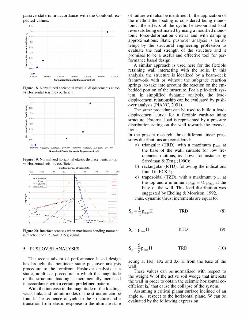
passive state is in accordance with the Coulomb ex-pected values.
0
0.05
0.1
0.15
0.2
0.25
0.3
0.35
0.4
0.45
0.0000% 0.5000% 1.0000% 1.5000% 2.0000% 2.5000% 3.0000%
Normalized Horizontal Displacement x/H
Seis
mic
Ho
rizo
nta
l C
oeff
icie
nt
kh
Figure 18. Normalized horizontal residual displacements at top vs Horizontal seismic coefficient.
0
0.05
0.1
0.15
0.2
0.25
0.3
0.35
0.4
0.45
0.00000% 0.00200% 0.00400% 0.00600% 0.00800% 0.01000% 0.01200% 0.01400%
Normalized Elastic Horizontal Displacement xel/H
Ho
rizo
nta
l S
eis
mic
Co
eff
icie
nt
kh
Figure 19. Normalized horizontal elastic displacements at top vs Horizontal seismic coefficient.
0
1
2
3
4
5
6
7
8
-200 -150 -100 -50 0 50 100 150 200
Interface normal stresses (kPa)
Dep
th (
m)
Numerical
At rest
Coulomb
EC8-5
Figure 20. Interface stresses when maximum bending moment is reached for a PGA=0.315 g signal.
5 PUSHOVER ANALYSES.
The recent advent of performance based design has brought the nonlinear static pushover analysis procedure to the forefront. Pushover analysis is a static, nonlinear procedure in which the magnitude of the structural loading is incrementally increased in accordance with a certain predefined pattern.
With the increase in the magnitude of the loading, weak links and failure modes of the structure can be found. The sequence of yield in the structure and a transition from elastic response to the ultimate state
of failure will also be identified. In the application of the method the loading is considered being mono-tonic: the effects of the cyclic behaviour and load reversals being estimated by using a modified mono-tonic force-deformation criteria and with damping approximations. Static pushover analysis is an at-tempt by the structural engineering profession to evaluate the real strength of the structure and it promises to be a useful and effective tool for per-formance based design.
A similar approach is used here for the flexible retaining wall interacting with the soils. In this analysis, the structure is idealized by a beam-deck framework with or without the subgrade reaction springs, to take into account the reaction on the em-bedded portion of the structure. For a pile-deck sys-tem, in simplified dynamic analysis, the load-displacement relationship can be evaluated by push-over analysis (PIANC, 2001).
The same procedure can be used to build a load-displacement curve for a flexible earth-retaining structure. External load is represented by a pressure distribution acting on the wall towards the excava-tion. In the present research, three different linear pres-sures distributions are considered:
a) triangular (TRD), with a maximum pmax at the base of the wall, suitable for low fre-quencies motions, as shown for instance by Steedman & Zeng (1990);
b) rectangular (RTD), following the indications found in EC8-5;
c) trapezoidal (TZD), with a maximum pmax at the top and a minimum pmin = ¼ pmax at the base of the wall. This load distribution was suggested by Ebeling & Morrison, 1992.
Thus, dynamic thrust increments are equal to:
Hp2
1S maxe = TRD (8)
HpS maxe = RTD (9)
Hp8
5S maxe = TRD (10)
acting at H/3, H/2 and 0.6 H from the base of the wall.
These values can be normalized with respect to the weight W of the active soil wedge that interests the wall in order to obtain the seismic horizontal co-efficient kh
* that cause the collapse of the system. Assuming a critical planar surface inclined of an
angle αcrit respect to the horizontal plane, W can be evaluated by the following expression
( )crit2 90tanH
2
1W α−°γ= (11)
Hence, the expressions of kh* are
( )crit
max*h 90tanH
pk
α−°γ= TRD (12)
( )crit
max*h 90tanH
p2k
α−°γ= RTD (13)
( )crit
max*h 90tanH4
p5k
α−°γ= TZD (14)
For a given geometry of a retaining wall, the value of kh
* can be obtained by static numerical analysis in which, starting from the system configu-ration after the excavation, an incremental load is applied on the structure until the failure is reached.
The aspects that should be considered in this type of analyses are:
a) geometrical nonlinearity: when the system reach the collapse the small deformations hypothesis is violated, hence, the calculation need continuous updating of the configura-tion;
b) material nonlinearity: the stress-strain behav-iour of the soil, the structural element, the soil-structure interface and the other ele-ments (anchors, props, etc.) must be repre-sented with suitable constitutive models that implement plasticity;
c) load advancement to the ultimate level: the external load must be applied incrementally in order to obtain a load-displacement rela-tionship that permits to detect the displace-ments of the system when is subjected to de-sign actions (seismic demand).
An example of application of this methodology is presented for the same RC cantilever diaphragm embedded in the homogeneous elasto-plastic layer, illustrated before. The analyses were conducted again with the FE code Plaxis.
5.1 Finite element model.
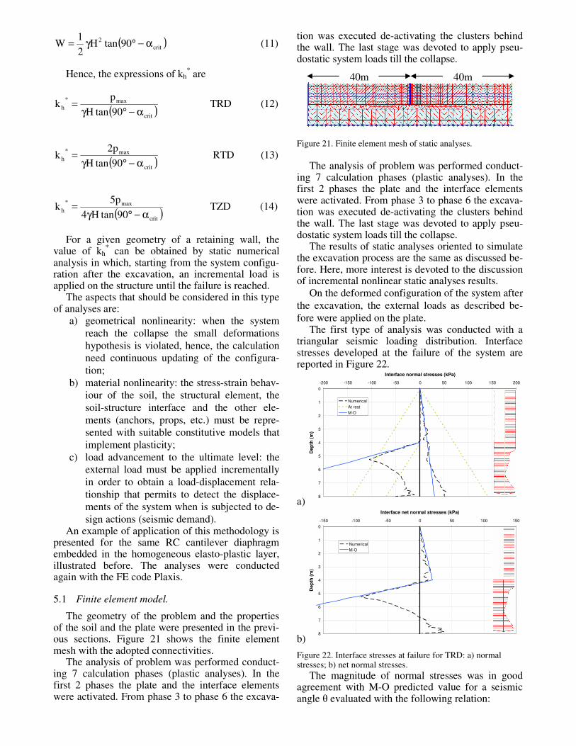
The geometry of the problem and the properties of the soil and the plate were presented in the previ-ous sections. Figure 21 shows the finite element mesh with the adopted connectivities.
The analysis of problem was performed conduct-ing 7 calculation phases (plastic analyses). In the first 2 phases the plate and the interface elements were activated. From phase 3 to phase 6 the excava-
tion was executed de-activating the clusters behind the wall. The last stage was devoted to apply pseu-dostatic system loads till the collapse.
Figure 21. Finite element mesh of static analyses.
The analysis of problem was performed conduct-
ing 7 calculation phases (plastic analyses). In the first 2 phases the plate and the interface elements were activated. From phase 3 to phase 6 the excava-tion was executed de-activating the clusters behind the wall. The last stage was devoted to apply pseu-dostatic system loads till the collapse.
The results of static analyses oriented to simulate the excavation process are the same as discussed be-fore. Here, more interest is devoted to the discussion of incremental nonlinear static analyses results.
On the deformed configuration of the system after the excavation, the external loads as described be-fore were applied on the plate.
The first type of analysis was conducted with a triangular seismic loading distribution. Interface stresses developed at the failure of the system are reported in Figure 22.
a)
0
1
2
3
4
5
6
7
8
-200 -150 -100 -50 0 50 100 150 200
Interface normal stresses (kPa)
Dep
th (
m)
Numerical
At rest
M-O
b)
0
1
2
3
4
5
6
7
8
-150 -100 -50 0 50 100 150
Interface net normal stresses (kPa)
Dep
th (
m)
Numerical
M-O
Figure 22. Interface stresses at failure for TRD: a) normal stresses; b) net normal stresses.
The magnitude of normal stresses was in good agreement with M-O predicted value for a seismic angle θ evaluated with the following relation:
40m 40m
( )hkarctan=θ (14)
kh is the ultimate value of seismic horizontal coeffi-cient reached in the analysis.
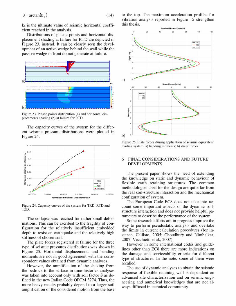
Distributions of plastic points and horizontal dis-placement shading at failure for RTD are depicted in Figure 23, instead. It can be clearly seen the devel-opment of an active wedge behind the wall while the passive wedge in front do not generate at failure.
a)
b)
Figure 23. Plastic points distribution (a) and horizontal dis-placements shading (b) at failure for RTD.
The capacity curves of the system for the differ-
ent seismic pressure distributions were plotted in Figure 24.
0
0.02
0.04
0.06
0.08
0.1
0.12
0.14
0.0000% 0.0050% 0.0100% 0.0150% 0.0200% 0.0250%
Normalized Horizontal Displacement x/H
Ho
rizo
nta
l S
eis
mic
Co
eff
icie
nt
kh
*
TRD
RTD
TZD
Collapse
Figure 24. Capacity curves of the system for TRD, RTD and TZD.
The collapse was reached for rather small defor-
mations. This can be ascribed to the fragility of con-figuration for the relatively insufficient embedded depth to resist an earthquake and the relatively high stiffness of chosen soil.
The plate forces registered at failure for the three type of seismic pressures distributions was shown in Figure 25. Horizontal displacements and bending moments are not in good agreement with the corre-spondent values obtained from dynamic analyses.
However, the amplification of the shaking from the bedrock to the surface in time-histories analyses was taken into account only with soil factor S as de-fined in the new Italian Code OPCM 3274. Thus, the more heavy results probably depend to a larger soil amplification of the considered motion from the base
to the top. The maximum acceleration profiles for vibration analysis reported in Figure 15 strengthen this thesis.
a)
0
1
2
3
4
5
6
7
8
0 20 40 60 80 100 120
Bending Moment (kNm/m)
De
pth
(m
)
TRD
RTD
TZD
b)
0
1
2
3
4
5
6
7
8
-60 -40 -20 0 20 40 60
Shear Forces (kN/m)
Dep
th (
m)
TRD
RTD
TZD
Figure 25. Plate forces during application of seismic equivalent loading system: a) bending moments; b) shear forces.
6 FINAL CONSIDERATIONS AND FUTURE DEVELOPMENTS.
The present paper shows the need of extending the knowledge on static and dynamic behaviour of flexible earth retaining structures. The common methodologies used for the design are quite far from the real soil-structure interaction and the mechanical configuration of system.
The European Code EC8 does not take into ac-count some important aspects of the dynamic soil-structure interaction and does not provide helpful pa-rameters to describe the performance of the system.
Some research efforts are in progress improve the way to perform pseudostatic analysis and overtake the limits in current calculation procedures (for in-stance, Callisto, 2005; Choudhury and Nimbalkar, 2007; Vecchietti et al., 2007).
However in some international codes and guide-lines other than EC8 there are more indications on the damage and serviceability criteria for different type of structures. In the note, some of them were recalled.
The use of dynamic analyses to obtain the seismic response of flexible retaining wall is dependent on advanced site characterization and on seismic engi-neering and numerical knowledges that are not al-ways diffused in technical community.

It is also necessary a good calibration of the model before conducting a dynamic analysis for any type of 2-D or 3-D geotechnical problem. Some pa-rameters (equivalent stiffness, numerical and mate-rial damping, etc.) can be chosen by comparing 1-D dynamic response of model to the theoretical or nu-merical solutions.
In the present work, an example of procedure to calibrate the finite element model parameters was presented.
Then, vibrations analysis has revealed that the first resonance frequency of the examined scheme is included between the natural frequencies of soil de-posits behind and in front of wall. Particularly, it is slightly larger than the first of these. The occurrence of plastic zones near to the structure involves a re-duction of maximum amplification ratio at the natu-ral frequency of the system. In presence of the exca-vation, maximum acceleration at surface is higher than the correspondent of free-field conditions.
The data obtained from the analyses with strong earthquakes have highlighted that the stability of system and plate forces reach the heavy conditions when the maximum displacement at top of wall is achieved. This displacement is a parameter more representative than the maximum acceleration to de-scribing the seismic behaviour of an embedded dia-phragm. Static and dynamic deformed configura-tions are composed by an elastic distortion of structural element and a rigid roto-translational mo-tion. For retaining structure with a flexural stiffness not very low, evaluation of earthquake induced dis-placements in the backfill can leave the elastic de-formations out of consideration.
On the other hand, a pseudostatic approach that permits to take into account nonlinearity of problem and soil-structure interaction was proposed. The procedure and a suggestion for the seismic load sys-tems to apply on the structure were illustrated. The results obtained are not well in agreement with the correspondents of dynamic analyses. This is proba-bly due to larger soil amplification from the base to the top of the model. In new Italian Code OPCM 3274 this aspect is considered with a soil factor S that represents the ratio of maximum accelerations at surface and at bedrock. It is referred to free field conditions and considers some relevant aspects of soil behaviour (stiffness degradation, damping evo-lution, etc.) not included in dynamic analyses of the present study. However, the application of pushover analyses to a flexible retaining structure seems to be an interesting procedure to describe behaviour of the system till to failure.
The example here presented is simple but it allow understanding some basic aspects on stress-strain re-
sponse of flexible retaining walls. However, the methodology will require the vali-
dation by means of more sophisticated dynamic analyses, centrifuge tests on scale model and case histories observations.
ACKNOWLEDGEMENTS.
The work presented in this paper is part of ReLUIS research project, founded by the Italian Department of Civil Protection.
REFERENCES
(pr)EN 1998-5 (2003). Eurocode 8: Design of structures for
earthquake resistance – Part 5: Foundations, retaining struc-tures and geotechnical aspects, CEN European Committee for Standardization, Bruxelles, Belgium.
Amorosi A.,Elia G., Boldini D., Sasso M., Lollino P. (2007). Sull’analisi della risposta sismica locale mediante codici di calcolo numerici. Proc. of IARG 2007 Salerno, Italy (in Italian).
Barrios D.B., Angelo E., Gonçalves E., (2005). Finite Element Shot Peening Simulation. Analysis and comparison with experimental results, MECOM 2005, VIII Congreso Argen-tino de Mecànica Computacional, Ed. A. Larreteguy, vol. XXIV, Buenos Aires, Argentina, Noviembre 2005
Brinkgreve R.B.J., Plaxis 2D version8. A.A. Balkema Pub-lisher, Lisse, 2002.
Callisto L. (2006). Pseudo-static seismic design of embedded retaining structures, Workshop of ETC12 Evaluation Committee for the Application of EC8, Athens, January 20-21.
Christian J.T., Roesset J.M., Desai C.S., (1977). Two- or Three-Dimensional Dynamic Analyses, Numerical Methods in Geotechnical Engineering, Chapter 20, pp. 683-718, Ed. Desai C.S., Christian J.T. - McGraw-Hill
Ebeling R.M., Morrison E.E.Jr. (1992). The seismic design of waterfront retaining structures, Technical Report ITL-92-11, US Army Engineers Waterways Experiment Station, Vicksburg, MS
Fourie A.B., Potts, D.M. (1989). Comparison of finite element and limiting equilibrium analyses for an embedded cantile-ver retaining wall, Geotechnique, vol.39, n.2, pp. 175-188
Kuhlmeyer R.L, Lysmer J. (1973). Finite Element Method Ac-curacy for Wave Propagation Problems, Journal of the Soil Mechanics and Foundation Division, vol.99 n.5, pp. 421-427
Lanzo G., Pagliaroli A., D’Elia B. (2004). L’influenza della modellazione di Rayleigh dello smorzamento viscoso nelle analisi di risposta sismica locale, ANIDIS, XI Congresso Nazionale “L’Ingegneria Sismica in Italia”, Genova 25-29 Gennaio 2004 (in Italian)
LUSAS (2000). Theory Manual, FEA Ltd., United Kingdom Lysmer J., Kuhlmeyer R.L. (1969). Finite Dynamic Model for
Infinite Media, ASCE, Journal of Engineering and Me-chanical Division, pp. 859-877
Ministry of Transport, Japan, 1999. Design Standard for Port and Harbour Facilities and Commentaries, Japan Port and Harbour Association, 1181 pp. (in Japanese)
OPCM n.3274 (2003). Primi elementi in material di criteri ge-nerali per la classificazione sismica del territorio nazionale e di normative tecniche per le costruzioni in zona sismica, Gazzetta Ufficiale della Repubblica Italiana, Vol.105, May 8th 2003 (in Italian)

Park D., Hashash Y.M.A. (2004). Soil Damping Formulation in Nonlinear Time Domain Site Response Analysis, Journal of Earthquake Engineering, vol.8 n.2, pp.249-274
PIANC (2001). Seismic Design Guidelines for Port Structures, Working Group n.34 of the Maritime Navigation Commis-sion, International Navigation Association, Balkema, Lisse, 474 pp.
Port and Harbour Research Institute, Japan (1997). Handbook on Liquefaction Remediation of Reclaimed Land, Transla-tion by US Army Corps of Engineers, Waterways Experi-ment Station), Balkema, 312 pp.
Roesset, J.M. (1970). Fundamentals of Soil Amplification, in: Seismic Design for. Nuclear Power Plants (R.J. Hansen, ed.), The MIT Press, Cambridge, MA, pp. 183-244.
Roesset J.M., (1977). Soil Amplification of Earthquakes, Nu-merical Methods in Geotechnical Engineering, Chapter 19, pp. 639-682, Ed. Desai C.S., Christian J.T. - McGraw-Hill
Ross M., (2004). Modeling Methods for Silent Boundaries in Infinite Media, ASEN 5519-006: Fluid-Structure Interac-tion, University of Colorado at Boulder
Steedman R.S., Zeng X. (1990)- The seismic response of wa-terfront retaining walls, Proc. ASCE Specialty Conference on Design and Performance of Earth Retaining Structures, Special Technical Publication 25, Cornell University, Ithaca, New York, pp.872-886
Werner S.D. (1998). Seismic Guidelines for Ports, Technical Council on Lifeline Earthquake Engineering, Monograph n.12, ASCE