Solving the One-Dimensional Wave Equation Part 2ramanujan.math.trinity.edu/rdaileda/teach/s14/m3357/lectures/... · BoundaryValueProblems D’Alembert’sSolution Examples Example

Boundary Value Problems D’Alembert’s Solution Examples

Solving the One-Dimensional Wave Equation

Part 2

Ryan C. Daileda

Trinity University

Partial Differential EquationsJanuary 28, 2014

Daileda The 1-D Wave Equation


The 1-D wave equation revisited

Recall: The one-dimensional wave equation

∂2u

∂t2= c2

∂2u

∂x2(1)

models the motion of an (ideal) string under tension.

Last time we saw that:

Theorem

The general solution to the wave equation (1) is

u(x , t) = F (x + ct) + G (x − ct),

where F and G are arbitrary (differentiable) functions of onevariable.



Remarks:

The solution is uniquely determined by the initial conditions

u(x , 0) = f (x), (2)

ut(x , 0) = g(x). (3)

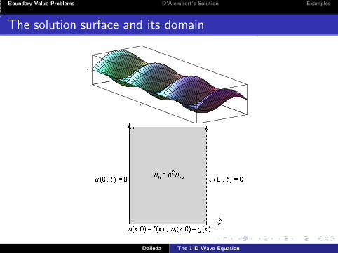
The domain of u(x , t) is

R = R× [0,∞).

The function u(x , t) satisfies:

∗ utt = c2uxx on the interior of R ;

∗ conditions (2) and (3) on the boundary of R .

This is an example of a boundary value problem.



The solution surface and its domain

uu

tt

xx



An additional boundary condition

We now assume that the vibrating string has finite length L, and isfixed at both ends.

The boundary value problem we now need to consider is

∂2u

∂t2= c2

∂2u

∂x2,

u(0, t) = u(L, t) = 0,

u(x , 0) = f (x),

ut(x , 0) = g(x),

on the domainR = [0, L] × [0,∞).



The solution surface and its domain

uu

tt

xx



D’Alembert’s solution of the vibrating string problem

We now turn to the solution of the (finite) vibrating string problem.

We would like to apply the general solution

u(x , t) = F (x + ct) + G (x − ct).

Problem: The initial conditions u(x , 0) = f (x) andut(x , 0) = g(x) only apply for

0 ≤ x ≤ L,

i.e. along the length of the string. But determining F and Grequires initial data for all x ∈ R.

Idea: Extend f and g (in some particular way) to all of R.



Periodic extensions

Given a function h(x) with domain [0, L] we first extend it to anodd function h1(x) on [−L, L] by reflecting its graph through theorigin:

Symbolically:

h1(x) =

h(x) if 0 < x ≤ L,

0 if x = 0,

−h(−x) if − L ≤ x < 0.



We then extend h1(x) to a function h∗(x) on all of R byrepeatedly “cutting and pasting” its graph:

This is called the 2L-periodic odd extension of h(x). Symbolically:

h∗(x) = h1

(

x − 2L

[x + L

2L

])

,

where [·] is the floor function.



Back to the vibrating string

Goal: Solve the wave equation∂2u

∂t2= c2

∂2u

∂x2on the domain

[0, L] × [0,∞), subject to the boundary conditions

u(0, t) = u(L, t) = 0,

u(x , 0) = f (x), ut(x , 0) = g(x).

Solution: We first use the 2L-periodic extensions of f and g andsolve the boundary value problem

∂2u

∂t2= c2

∂2u

∂x2,

u(x , 0) = f ∗(x), ut(x , 0) = g∗(x),

on R× [0,∞). Then we show that for 0 ≤ x ≤ L, this u(x , t)solves the vibrating string problem.



For 0 ≤ x ≤ L, we immediately have

u(x , 0) = f ∗(x) = f (x),

ut(x , 0) = g∗(x) = g(x).

To verify the other boundary conditions, we write

u(x , t) = F (x + ct) + G (x − ct)

and solve for F and G . We find that

f ∗(x) = u(x , 0) = F (x) + G (x),

(f ∗)′(x) = F ′(x) + G ′(x),

g∗(x) = ut(x , 0) = cF ′(x)− cG ′(x).



The last two equations are equivalent to

(1 1c −c

)(F ′

G ′

)

=

((f ∗)′

g∗

)

.

Matrix inversion gives

(F ′

G ′

)

=−1

2c

(−c −1−c 1

)((f ∗)′

g∗

)

=

(f ∗)′

2+

g∗

2c

(f ∗)′

2−

g∗

2c

Therefore, by FTOC,

F (x + ct)− F (0) =

∫x+ct

0

F ′(s) ds =

∫x+ct

0

(f ∗)′(s)

2+

g∗(s)

2cds

=1

2(f ∗(x + ct)− f ∗(0)) +

1

2c

∫x+ct

0

g∗(s) ds.



Likewise, one can show

G (x − ct)− G (0) =1

2(f ∗(x − ct)− f ∗(0)) −

1

2c

∫x−ct

0

g∗(s) ds

=1

2(f ∗(x − ct)− f ∗(0)) +

1

2c

∫ 0

x−ct

g∗(s) ds.

Since f ∗(0) = 0 and f ∗(x) = F (x) + G (x), it now follows that

u(x , t) = F (x + ct) + G (x − ct)

= F (0) + G (0) +f ∗(x + ct) + f ∗(x − ct)

2+

1

2c

∫x+ct

x−ct

g∗(s) ds

=f ∗(x + ct) + f ∗(x − ct)

2+

1

2c

∫x+ct

x−ct

g∗(s) ds.



It remains to show that u(0, t) = u(L, t) = 0 for all t > 0.

Setting x = 0 in the expression above yields

u(0, t) =f ∗(ct) + f ∗(−ct)

2+

1

2c

∫ct

−ct

g∗(s) ds = 0

since f ∗ and g∗ are both odd functions.

Setting x = L we get

u(L, t) =f ∗(L+ ct) + f ∗(L− ct)

2︸︷︷︸

A

+1

2c

∫L+ct

L−ct

g∗(s) ds

︸︷︷︸

B

.

Because f ∗ and g∗ are both 2L-periodic and odd, one can showthat A = B = 0 (HW), which finishes our work.



Summary

Theorem (D’Alembert)

The solution of the vibrating string problem

∂2u

∂t2= c2

∂2u

∂x2,

u(0, t) = u(L, t) = 0,

u(x , 0) = f (x), ut(x , 0) = g(x).

on the domain [0, L] × [0,∞) is given by

u(x , t) =f ∗(x + ct) + f ∗(x − ct)

2+

1

2c

∫x+ct

x−ct

g∗(s) ds,

where f ∗ and g∗ are the 2L-periodic odd extensions of f and g.

Remark: One can show that, in fact, this solution is unique.Daileda The 1-D Wave Equation


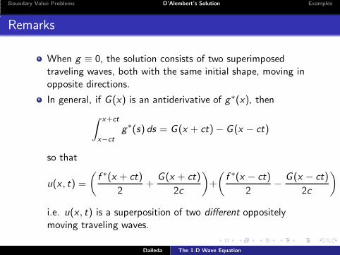
Remarks

When g ≡ 0, the solution consists of two superimposedtraveling waves, both with the same initial shape, moving inopposite directions.

In general, if G (x) is an antiderivative of g∗(x), then

∫x+ct

x−ct

g∗(s) ds = G (x + ct)− G (x − ct)

so that

u(x , t) =

(f ∗(x + ct)

2+

G (x + ct)

2c

)

+

(f ∗(x − ct)

2−

G (x − ct)

2c

)

,

i.e. u(x , t) is a superposition of two different oppositelymoving traveling waves.



Example

Show that the solution to the vibrating string problem is periodicin time, with period 2L/c. That is, show that if u(x , t) is asolution, then

u(x , t + 2L/c) = u(x , t).

First, if a function h has period 2L, we have

h(x ± c(t + 2L/c)) = h(x ± ct ± 2L) = h(x ± ct),

which shows that h(x ± ct) has period 2L/c in t.

The solution u(x , t) is built of functions of the form h(x ± ct),with h = f ∗,G .

So, it suffices to show that f ∗ and G have period 2L.



By definition, f ∗ has period 2L.

According to the FTOC

G (x + 2L) − G (x) =

∫x+2L

x

g∗(s) ds =

∫L

−L

g∗(s) ds = 0,

since g∗ is 2L-periodic and odd. This shows

G (x + 2L) = G (x),

which is what we wanted to show.

Remark: The fact that G (x) is 2L-periodic is independently useful.



Example

Solve the vibrating string problem with L = c = 1, f (x) = x(1− x)and g(x) = 1− x.

We first find f ∗(x). The odd extension of f to [−1, 1] is

f1(x) =

x(x + 1) if − 1 ≤ x < 0,

0 if x = 0,

x(x − 1) if 0 < x ≤ 1.

Hence

f ∗(x) = f1

(

x − 2

[x + 1

2

])

.



The odd extension of g to [−1, 1] is

g1(x) =

−1− x if − 1 ≤ x < 0,

0 if x = 0,

1− x if 0 < x ≤ 1.

.

Now we need an antiderivative of g1. For x ∈ [−1, 0] we have

G1(x) =

∫x

−1

g1(s) ds =

∫x

−1

−1− s ds = −x2

2− x −

1

2,

and for x ∈ [0, 1] we have

G1(x) =

∫x

−1

g1(s) ds =

∫ 0

−1

g1(s) ds+

∫x

0

1− s ds = −x2

2+x−

1

2.



The function G is then the 2-periodic extension of G1:

G (x) = G1

(

x − 2

[x + 1

2

])

.

Here are the graphs of g∗ (in blue) and G (in red):

Since c = 1, the solution is then

u(x , t) =f ∗(x + t) + G (x + t)

2+

f ∗(x − t)− G (x − t)

2.



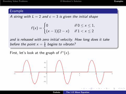
Example

A string with L = 2 and c = 3 is given the initial shape

f (x) =

{

0 if 0 ≤ x ≤ 1,

(x − 1)(2− x) if 1 < x ≤ 2

and is released with zero initial velocity. How long does it takebefore the point x = 1

5begins to vibrate?

First, let’s look at the graph of f ∗(x).



Since g ≡ 0, the solution u(x , t) is a superposition two copies off ∗, one moving left, the other right, with speed c = 3.

The graph shows that the left-moving copy reaches x = 15first.

The vibration must move 1− 15= 4

5of a unit to reach x = 1

5.

Thus, the amount of time it takes for this to happen is

t =4/5

3=

4

15.


Documents

Solving the One-Dimensional Wave Equation Part 2ramanujan.math.trinity.edu/rdaileda/teach/s14/m3357/lectures/... · BoundaryValueProblems D’Alembert’sSolution Examples Example