Solving Stochastic Dynamic Programming Problems:

a Mixed Complementarity Approach

Wonjun Chang, Thomas F. Rutherford∗

Department of Agricultural and Applied Economics

Optimization Group, Wisconsin Institute for Discovery

University of Wisconsin-Madison

Abstract

We present a mixed complementarity problem (MCP) formulation of infinite horizon dy-

namic programming (DP) problems with continuous state space. The MCP approach

replaces conventional value function iteration by the solution of a one-shot square sys-

tem of equations and inequalities. Three numerical examples illustrate our approach and

demonstrate that the DP-MCP algorithm can compute equilibria much faster than tradi-

tional value iteration. In addition, the MCP approach accommodates corner solutions in

the optimal policy.

Keywords: Dynamic Programming; Stochastic Dynamic Programming, Computable Gen-

eral Equilibrium, Complementarity, Computational Methods, Natural Resource Manage-

ment; Integrated Assessment Models

This research was partially supported by the Electric Power Research Institute (EPRI). We would like toacknowledge the input of Richard Howitt, Youngdae Kim and the Optimization Group at UW-Madison forhelpful comments and discussion. We also thank Wouter den Haan for his lectures and homework assignmentsin the Macroeconomics Summer School at the London School of Economics (2014).

∗Corresponding Author: Tel. +1 (608) 890-4576E-mail: rutherford@aae.wisc.edu

1

1. Introduction

Dynamic programming (DP) is a standard tool in solving dynamic optimization problems due

to the simple yet flexible recursive feature embodied in Bellman’s equation [Bellman, 1957].

In the conventional method, a DP problem is decomposed into simpler subproblems char-

acterized by a small set of state variables for which an optimal decision rule —a predefined

function of the state variables —can be found at every stage. For stochastic dynamic prob-

lems in particular, DP is a powerful optimization principle, and for some stochastic problem

types, DP serves as the only tractable solution method [Lontzek et al., 2012]. Methodolog-

ical advances in approximation theory and numerical integration to overcome the so-called

curse of dimensionality and to extend DP to problems that cannot be solved analytically,

has encouraged the use of numerical DP methods, especially in economics [Judd, 1998, Rust,

1996, Maliar and Maliar, 2015, Manuelli and Sargent, 2009, Wright and Nocedal, 1999, Powell,

2011]. Complementarity programming also had a long history in economics with a formula-

tion appearing in Scarf et al. [1967] and numerical tools introduced by rut [1995] and Ferris

and Munson [2000].

Unlike the optimization algorithms in mathematical programming, there is no standard

formulation of a DP problem, nor is there an off-the-shelf solver package designated specifi-

cally for DP (as the simplex method is for linear programming problems) [Brandimarte, 2014].

DP is a principle, and there exist multiple formulations and customizations that focus on solu-

tion accuracy and computational efficiency when it comes to implementation [Tauchen, 1986,

Cai and Judd, 2015, Judd et al., 2014].

Among various settings of dynamic programming problems, we focus on solving infinite

horizon DP problems with continuous state and control variables. Value function iteration

and policy function iteration are the two common computational approaches taken in such

settings, mainly due to the algorithms’ monotonic convergence properties and straightfor-

ward implementation. Despite their stability, the iterative aspect of these nonlinear pro-

gramming (NLP) based algorithms make DP implementation time consuming, as processing

time increases quickly in grid size for large multi-state applications, often rendering them

intractable by the curse of dimensionality.

The mixed complementarity approach (MCP) introduced in this paper omits the iterative

aspect of conventional NLP based DP implementations, to significantly reduce the run-time

required to solve the DP problem and extend the application of dynamic programming to

problems that are computationally burdensome. The MCP that corresponds to the value

function iteration procedure is a square system of equilibrium constraints that consist of:

2

a. Bellman’s optimality conditions with respect to the vector of control variables, x;

b. optimality conditions for least squares fitting of value function parameters, α;

for which the solution is a pair (x, α) that characterizes a Nash equilibrium with respect

to the two objectives. For the latter objective, this means that in the case that the value

function, V(x ; α), is estimated using polynomials, optimal parameterization of α would cor-

respond to determining the polynomial coefficients that would obtain once the polynomial

approximation converges by the contraction mapping theorem in the iterative scheme. More

importantly, computational advantages set aside, the MCP approach allows for the proper

treatment of corner solutions while solving for the optimal policy [Balistreri, 1999].

Our interest in the use of complementarity methods for solving dynamic programming

problems was inspired by the work of Dubé et al. [2012], Su and Judd [2012]. Their papers fo-

cus on structural estimation of discrete choice problems. Our objective is to demonstrate how

their equilibrium programming approach can be extended to a continous choice problems

featuring explicit complementary slackness conditions. We lay out three sample applications

and argue that a mixed complementarity formulation is intuitive, robust and efficient for

finding optimal policies. We stop short of showing how this approach could be applied for

stuctural estimation methods, although it seems likely that Su and Judd [2012]’s ideas could

be directly employed.

Following Richard Howitt’s “Betty Crocker” approach to Dynamic Programming [Howitt

et al., 2002a]—a pedagogic paper which makes DP more accessible to empirical economists

through straightforward numerical examples—we solve various versions of the standard neo-

classical growth model in GAMS to show that the one-shot MCP approach completes the

value approximation procedure in a fraction of the run time required by all iterative NLP

methods. We furthermore demonstrate the helpfulness of using orthogonal polynomials to

improve the accuracy of the deterministic DP solution, and the use of numerical integration

techniques to extend the one-shot formulation to stochastic DP problems.

The paper is organized as follows. Section 2 introduces the traditional value iteration

approach in solving an infinite-horizon DP problem. Section 3 presents the corresponding

DP-MCP formulation. In sections 4 and 5, we provide simple numerical examples of deter-

ministic and stochastic optimal growth models, including a single region, 3-sector stochastic

growth model based on Global Trade Analysis Project (GTAP) data to demonstrate the com-

putational advantages of DP-MCP. In the last section, we solve a stochastic natural resource

management problem in Hydropower planning to derive optimal policies consistent with

corner solutions; a key objective of the complementarity approach.

3

2. The Value Iteration Approach

The value function iteration procedure is the workhorse of many expository papers aimed to

make numerical DP more accessible [Howitt et al., 2002a, Aruoba and Fernández-Villaverde,

2014, Manuelli and Sargent, 2009, Sargent and Stachurski, 2015]. Given an estimate of the

value function, Vn(x), as a function of state variable x, the value iteration approach computes

an updated estimate of the value function using the Bellman equation, i.e.:

Vn+1(x) = maxa∈A

[C(x, a) + βVn(x

′)

]

where A is the action space and C, the immediate contribution function. The solution to

this iterative scheme converges monotonically to the true solution of the fixed point problem,

provided concavity of C and sufficient iterations of the procedure.

Traditionally based on standard nonlinear programming, the value iteration method is

stable, yet due to the iterative aspect of the algorithm, is slow and time consuming. Finding

all equilibria quickly becomes a daunting computational task as we increase the number state

variables and grid points. In fact, computing time increases exponentially in grid size, render-

ing large multi-state DP applications intractable by the curse of dimensionality. As a result,

complicated models that have difficulty employing recursive optimization have resorted to

either simulation or math programming based stochastic frameworks [Chang, 2016].

The Bellman equation for the general deterministic infinite horizon DP problem with

continuous state variables is stated as follows:

Vt(x) = maxa∈A(x)

Ct(x, a) + βVt+1(x′)

s.t. x′= h(x, a)

where x is the continuous state, a, the control variable and x′, the next-stage continuous state

with transition function h.

Algorithm. Value Function Iteration for Infinite Horizon Problems

1. Set m grid points and a functional form for V(x ; α);

for ∀i ≤ m, choose approximation nodes xi ∈ X;

fix a tolerance parameter ε;

denote Vn(x) to be value estimate output for iteration count n.

2. Initialize estimate of value function V0(x).

4

3. For n ≥ 1: obtain parameters αn−1 s.t. V(xi ; αn−1) = Vn−1(xi)

→ solve minαn−1

[∑i

(Vn−1(xi)−V(xi ; αn−1)2

]4. For ∀i, compute:

Vn(xi) = maxa∈A

[C(xi, a) + βV(x

′i ; αn−1)

]5. If ‖Vn −Vn−1‖ < ε(1− β)/2β, stop;

else set n = n + 1 and go to step 3.

The algorithm seeks an approximation to the value function, such that the sum of the

maximized contribution and the discounted next period value based on the approximated

function, maximizes the total value function [Howitt et al., 2002a]. The value iteration procedure

solves for two objectives. The optimization objective in step 3 is to minimize the square

deviation between estimated total value at grid points and the approximating value function.

The other objective displayed in step 4, is to optimize the control variable such that the

Bellman relationship holds. Convergence of the iterative approximation sequence generated

by the relationship, Vn+1 = TVn, where T is the Bellman operator, is guaranteed by the

contraction mapping theorem [Stokey and Lucas Jr, 1989].

3. DP-MCP: Dynamic Programming as a Mixed Complementarity Problem

We convert the value iteration process, a nonlinear optimization problem, into a nonlinear

complementarity problem, a square system of equations and inequalities for which a well-

established complementarity problem solver such as PATH can be applied [Ferris and Mun-

son, 2000, Dirkse and Ferris, 1995]. The main advantage of employing a complementarity

format is that it provides a simple method for incorporating inequality constraints and com-

plementary slackness conditions. The optimization objective in our case is to find an ap-

proximation to the value function, such that the value function is maximized when Bellman’s

principle of optimality holds. The idea then is to solve the approximation problem simulta-

neously with the optimality conditions, to construct a one-shot solution to the DP problem as

a complementarity problem, without resorting to value function iteration.

We note however that the complementarity formulation encompasses both primal and

dual variables, doubling the number of equations. The objective of this paper is thus largely

pedagogic despite the simplicity of the idea the problem reformulation is based on. The

5

Extended Mathematical Programming (EMP) framework in GAMS functions as a useful re-

source for such non-standard models that require reformulation into more accessible models

of established math programming classes [Ferris et al., 2009, Ferris and Sinapiromsaran, 2000].

Notice that we can write the maximization stage (step 4) of the value iteration procedure

in terms of the first order conditions (FOC) of the control variable as follows:

maxa∈A

[C(xi, a) + βV(x

′i ; αn−1)

]−→ ∂C(xi, a)

∂a+ β

∂V(x′i ; αn−1)

∂a≤ 0, ∀i ∈ 1, · · · , m

Similarly, the step for function fitting by means of least-squares estimation can also be written

in terms of its corresponding FOCs for ∀n, for which we define α = [α0, · · · , αk] to be a vector

of k coefficients used to parameterize the value function estimation.

minαn−1

[∑

i

(Vn−1(xi)−V(xi ; αn−1)

)2]−→ ∇αn−1

[∑

i

(Vn−1(xi)−V(xi ; αn−1)

)2]= 0

We now cast the value iteration problem as a complementarity problem by solving the maxi-

mization problem simultaneously with the least-squares function estimation problem in com-

plementarity form. The system of inequalities and equations that make up the MCP becomes:

MCP Formulation for Deterministic Infinite Horizon DP

∂C(xi, a)∂a

+ β∂V(x

′i ; α)

∂a≤ pi ⊥ a ≥ 0, ∀i

Ui = C(xi, a) + βV(x′i ; α) ⊥ Ui is free, ∀i

∂ ∑i

(Ui −V(xi ; α)

)2

∂αl= 0 ⊥ αl is free, ∀l ∈ 0, · · · , k

x′i = h(xi, a) ⊥ pi is free, ∀i

For the stochastic case, we can write the Bellman equation for the DP problem as follows:

Vt(x) = maxa∈A(x)

Ct(x, ω, a) + βE

Vt+1(x′, ω

′)|x, ω, a

s.t. x

′= h(x, ω, a)

where the transition function h now includes a stochastic element ω ∈ Ω. The corresponding

value function iteration procedure becomes:

6

Algorithm. Value Function Iteration for Stochastic Infinite Horizon Problems

1. Set m grid points and functional form for V(x, ω ; α);

for all grid points (i, j) choose approximation nodes xi ∈ X, ωj ∈ Ω;

fix a tolerance parameter ε;

denote Vn(x, ω) to be value estimate output for iteration count n.

2. Initialize estimate of value function V0(x, ω).

3. For n ≥ 1: obtain parameters αn−1 s.t. V(xi, ωj ; αn−1) = Vn−1(xi, ωj)

→ solve minαn−1

[∑i

(Vn−1(xi, ωj)−V(xi, ωj ; αn−1)2

]4. For ∀(i, j), compute:

Vn(xi, ωj) = maxa∈A

[C(xiωj, a) + βE

V(x

′ij, ω

′; αn−1)|xj, ωj, a

]5. If ‖Vn −Vn−1‖ < ε(1− β)/2β, stop;

else set n = n + 1 and go to step 3.

for which the corresponding MCP system of equations and inequalities is as follows:

MCP Formulation for Stochastic Infinite Horizon DP

∂C(xi, ωj, a)∂a

+ β∂E

V(x′ij, ω

′; α)|xi, ωj, a

∂a

≤ pij ⊥ a ≥ 0, ∀(i, j)

Uij = C(xi, ωj, a) + βE

V(x′ij, ω

′; α)|xi, ωj, a

⊥ Uij is free, ∀(i, j)

∂ ∑i,j

(Uij −V(xi, ωj ; α)

)2

∂αl= 0 ⊥ αl is free, ∀l ∈ 0, · · · , k

x′ij = h(xi, ωj, a) ⊥ pij is free, ∀(i, j)

7

4. The Brock-Mirman Stochastic Growth Model

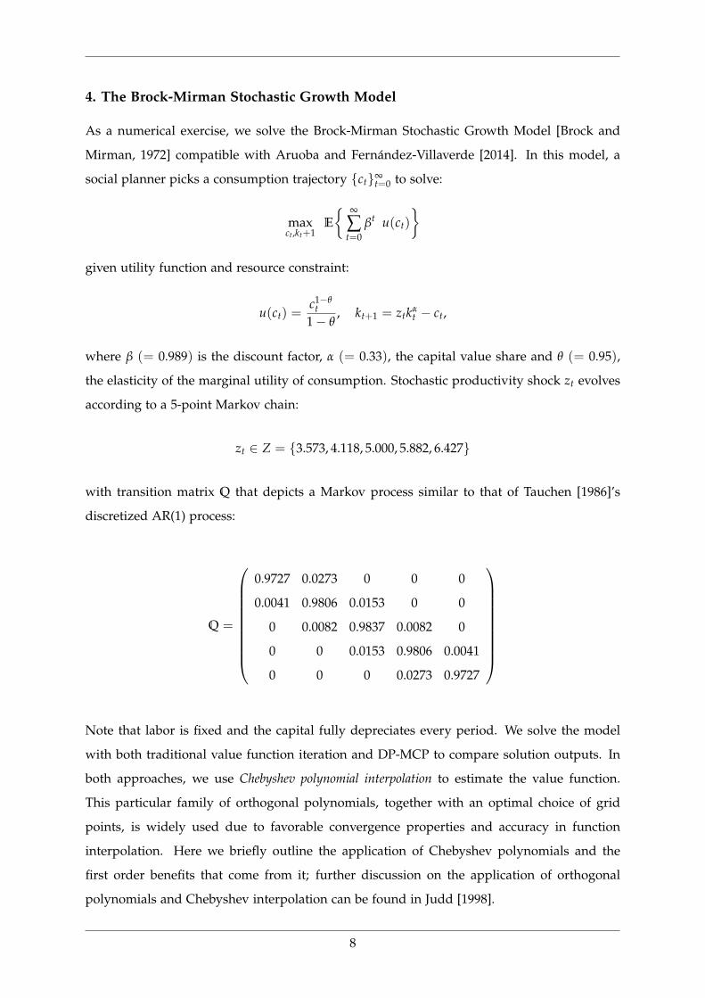
As a numerical exercise, we solve the Brock-Mirman Stochastic Growth Model [Brock and

Mirman, 1972] compatible with Aruoba and Fernández-Villaverde [2014]. In this model, a

social planner picks a consumption trajectory ct∞t=0 to solve:

maxct,kt+1

E

∞

∑t=0

βt u(ct)

given utility function and resource constraint:

u(ct) =c1−θ

t1− θ

, kt+1 = ztkαt − ct,

where β (= 0.989) is the discount factor, α (= 0.33), the capital value share and θ (= 0.95),

the elasticity of the marginal utility of consumption. Stochastic productivity shock zt evolves

according to a 5-point Markov chain:

zt ∈ Z = 3.573, 4.118, 5.000, 5.882, 6.427

with transition matrix Q that depicts a Markov process similar to that of Tauchen [1986]’s

discretized AR(1) process:

Q =

0.9727 0.0273 0 0 0

0.0041 0.9806 0.0153 0 0

0 0.0082 0.9837 0.0082 0

0 0 0.0153 0.9806 0.0041

0 0 0 0.0273 0.9727

Note that labor is fixed and the capital fully depreciates every period. We solve the model

with both traditional value function iteration and DP-MCP to compare solution outputs. In

both approaches, we use Chebyshev polynomial interpolation to estimate the value function.

This particular family of orthogonal polynomials, together with an optimal choice of grid

points, is widely used due to favorable convergence properties and accuracy in function

interpolation. Here we briefly outline the application of Chebyshev polynomials and the

first order benefits that come from it; further discussion on the application of orthogonal

polynomials and Chebyshev interpolation can be found in Judd [1998].

8

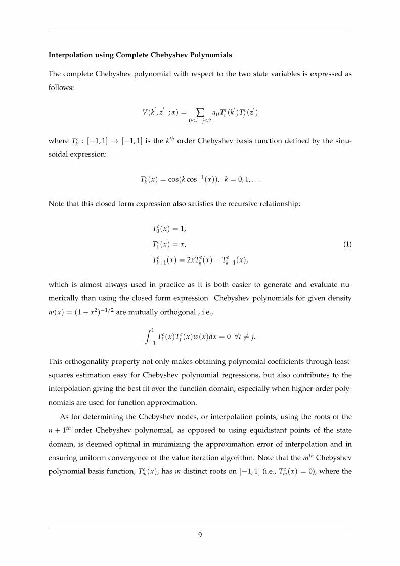
Interpolation using Complete Chebyshev Polynomials

The complete Chebyshev polynomial with respect to the two state variables is expressed as

follows:

V(k′, z′

; α) = ∑0≤i+j≤2

aijTci (k

′)Tc

j (z′)

where Tck : [−1, 1] → [−1, 1] is the kth order Chebyshev basis function defined by the sinu-

soidal expression:

Tck (x) = cos(k cos−1(x)), k = 0, 1, . . .

Note that this closed form expression also satisfies the recursive relationship:

Tc0(x) = 1,

Tc1(x) = x, (1)

Tck+1(x) = 2xTc

k (x)− Tck−1(x),

which is almost always used in practice as it is both easier to generate and evaluate nu-

merically than using the closed form expression. Chebyshev polynomials for given density

w(x) = (1− x2)−1/2 are mutually orthogonal , i.e.,

∫ 1

−1Tc

i (x)Tcj (x)w(x)dx = 0 ∀i 6= j.

This orthogonality property not only makes obtaining polynomial coefficients through least-

squares estimation easy for Chebyshev polynomial regressions, but also contributes to the

interpolation giving the best fit over the function domain, especially when higher-order poly-

nomials are used for function approximation.

As for determining the Chebyshev nodes, or interpolation points; using the roots of the

n + 1th order Chebyshev polynomial, as opposed to using equidistant points of the state

domain, is deemed optimal in minimizing the approximation error of interpolation and in

ensuring uniform convergence of the value iteration algorithm. Note that the mth Chebyshev

polynomial basis function, Tcm(x), has m distinct roots on [−1, 1] (i.e., Tc

m(x) = 0), where the

9

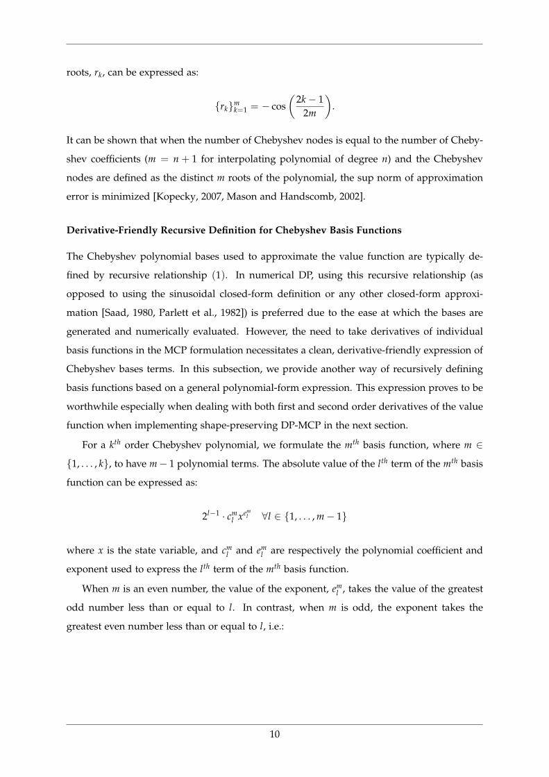
roots, rk, can be expressed as:

rkmk=1 = − cos

(2k− 1

2m

).

It can be shown that when the number of Chebyshev nodes is equal to the number of Cheby-

shev coefficients (m = n + 1 for interpolating polynomial of degree n) and the Chebyshev

nodes are defined as the distinct m roots of the polynomial, the sup norm of approximation

error is minimized [Kopecky, 2007, Mason and Handscomb, 2002].

Derivative-Friendly Recursive Definition for Chebyshev Basis Functions

The Chebyshev polynomial bases used to approximate the value function are typically de-

fined by recursive relationship (1). In numerical DP, using this recursive relationship (as

opposed to using the sinusoidal closed-form definition or any other closed-form approxi-

mation [Saad, 1980, Parlett et al., 1982]) is preferred due to the ease at which the bases are

generated and numerically evaluated. However, the need to take derivatives of individual

basis functions in the MCP formulation necessitates a clean, derivative-friendly expression of

Chebyshev bases terms. In this subsection, we provide another way of recursively defining

basis functions based on a general polynomial-form expression. This expression proves to be

worthwhile especially when dealing with both first and second order derivatives of the value

function when implementing shape-preserving DP-MCP in the next section.

For a kth order Chebyshev polynomial, we formulate the mth basis function, where m ∈

1, . . . , k, to have m− 1 polynomial terms. The absolute value of the lth term of the mth basis

function can be expressed as:

2l−1 · cml xem

l ∀l ∈ 1, . . . , m− 1

where x is the state variable, and cml and em

l are respectively the polynomial coefficient and

exponent used to express the lth term of the mth basis function.

When m is an even number, the value of the exponent, eml , takes the value of the greatest

odd number less than or equal to l. In contrast, when m is odd, the exponent takes the

greatest even number less than or equal to l, i.e.:

10

m is even m is odd

em1

em2

= 1 em1 = 0

em3

em4

= 3em

2

em3

= 2

......

We can define the coefficients cml recursively using the following recursive relation:

cmm−1 = 1

cmm−r =

cm−1

m−r+1 if r ∈ 2, . . . , m− 1 is even

cm−1m−r−1 + cm−2

m−r if r ∈ 2, . . . , m− 1 is odd

And lastly, in writing the mth basis function as a function of m− 1 polynomial terms, the sign

of each polynomial term alternates as a function of the state variable exponent, eml . Starting

with the polynomial term with the highest power, which takes a positive sign, the sign of

each polynomial term alternates as we decrement the exponent by two each time.

To demonstrate the construction of basis functions using the specified recursive relation-

ship, we write out the 6th-order Chebyshev polynomial basis functions in general polynomial

form:

m l = 5 l = 4 l = 3 l = 2 l = 1

1 1

2 x

3 2 · x2 −1

4 22 · x3 −2 · x −1 · x

5 23 · x4 −22 · x2 −2 · 2x2 +1

6 24 · x5 −23 · x3 −22 · 3x3 +2 · 2x +1 · x

Table 1. Derivative-Friendly Basis Functions

for 6th order Chebyshev Polynomial

11

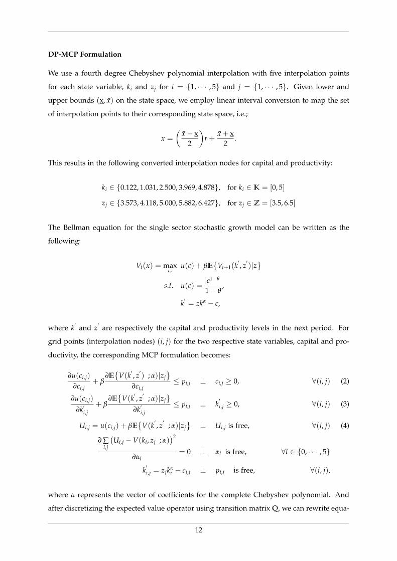
DP-MCP Formulation

We use a fourth degree Chebyshev polynomial interpolation with five interpolation points

for each state variable, ki and zj for i = 1, · · · , 5 and j = 1, · · · , 5. Given lower and

upper bounds (x, x) on the state space, we employ linear interval conversion to map the set

of interpolation points to their corresponding state space, i.e.;

x =

(x− x

2

)r +

x + x2

.

This results in the following converted interpolation nodes for capital and productivity:

ki ∈ 0.122, 1.031, 2.500, 3.969, 4.878, for ki ∈ K = [0, 5]

zj ∈ 3.573, 4.118, 5.000, 5.882, 6.427, for zj ∈ Z = [3.5, 6.5]

The Bellman equation for the single sector stochastic growth model can be written as the

following:

Vt(x) = maxct

u(c) + βE

Vt+1(k′, z′)|z

s.t. u(c) =c1−θ

1− θ,

k′= zkα − c,

where k′

and z′

are respectively the capital and productivity levels in the next period. For

grid points (interpolation nodes) (i, j) for the two respective state variables, capital and pro-

ductivity, the corresponding MCP formulation becomes:

∂u(ci,j)

∂ci,j+ β

∂E

V(k′, z′) ; α)|zj

∂ci,j

≤ pi,j ⊥ ci,j ≥ 0, ∀(i, j) (2)

∂u(ci,j)

∂k′i,j+ β

∂E

V(k′, z′

; α)|zj

∂k′i,j≤ pi,j ⊥ k

′i,j ≥ 0, ∀(i, j) (3)

Ui,j = u(ci,j) + βE

V(k′, z′

; α)|zj⊥ Ui,j is free, ∀(i, j) (4)

∂ ∑i,j

(Ui,j −V(ki, zj ; α)

)2

∂αl= 0 ⊥ αl is free, ∀l ∈ 0, · · · , 5

k′i,j = zjkα

i − ci,j ⊥ pi,j is free, ∀(i, j),

where α represents the vector of coefficients for the complete Chebyshev polynomial. And

after discretizing the expected value operator using transition matrix Q, we can rewrite equa-

12

tions (2)− (4) as:

∂u(ci,j)

∂ci,j+ β

∂ ∑j′ q(j, j′) ·V(k

′, z′

; α)

∂ci,j≤ pi,j ⊥ ci,j ≥ 0, ∀(i, j)

∂u(ci,j)

∂k′i,j+ β

∂ ∑j′ q(j, j′) ·V(k

′, z′

; α)

∂k′i,j≤ pi,j ⊥ k

′i,j ≥ 0, ∀(i, j)

Ui,j = u(ci,j) + β ∑j′

q(j, j′) ·V(k

′, z′

; α) ⊥ Ui,j is free, ∀(i, j)

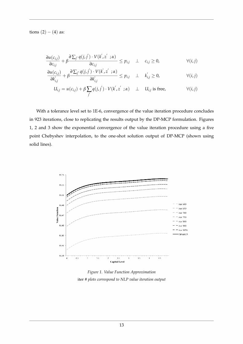
With a tolerance level set to 1E-6, convergence of the value iteration procedure concludes

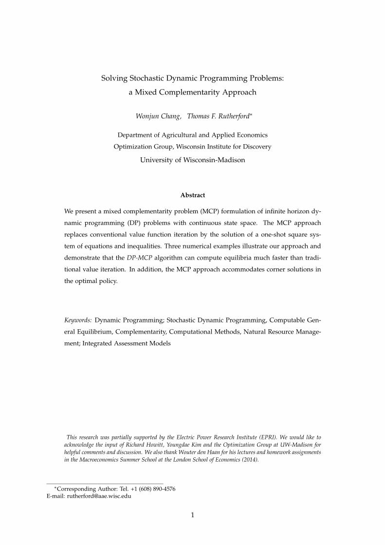
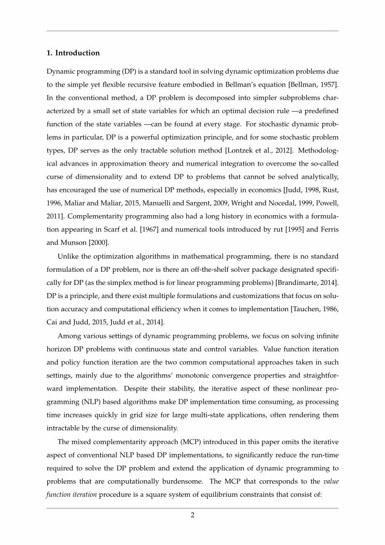
in 923 iterations, close to replicating the results output by the DP-MCP formulation. Figures

1, 2 and 3 show the exponential convergence of the value iteration procedure using a five

point Chebyshev interpolation, to the one-shot solution output of DP-MCP (shown using

solid lines).

Figure 1. Value Function Approximation

iter # plots correspond to NLP value iteration output

13

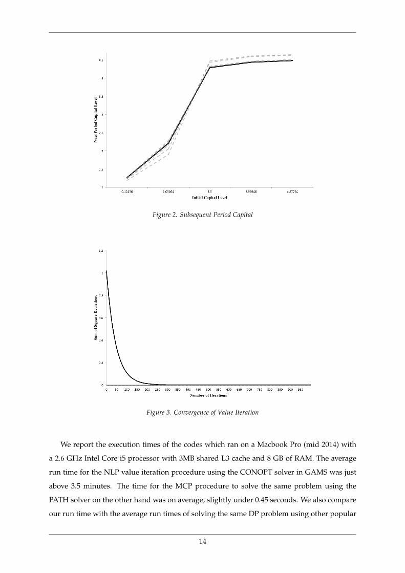
Figure 2. Subsequent Period Capital

Figure 3. Convergence of Value Iteration

We report the execution times of the codes which ran on a Macbook Pro (mid 2014) with

a 2.6 GHz Intel Core i5 processor with 3MB shared L3 cache and 8 GB of RAM. The average

run time for the NLP value iteration procedure using the CONOPT solver in GAMS was just

above 3.5 minutes. The time for the MCP procedure to solve the same problem using the

PATH solver on the other hand was on average, slightly under 0.45 seconds. We also compare

our run time with the average run times of solving the same DP problem using other popular

14

programming languages such as C++ and Fortran, as presented in Aruoba and Fernández-

Villaverde [2014]. We find that solving DP-MCP with PATH on GAMS is notably faster than

solving DP-NLP using any of the programs listed in the paper.

5. N-Sector Stochastic Growth Model

In this section we incorporate multiple sectors to the stochastic growth model, with perfectly

correlated productivity shocks across sectors that follow a first-order autoregressive (AR1)

process. A social planner chooses the consumption trajectory, cst∞

t=0, investment trajectory,

Ist ∞

t=0, and labor supply trajectory, Lst∞

t=0, to solve the following optimization problem:

maxcs

t ,Ist ,Ys

t E

[ ∞

∑t=0

βt u(c1t , · · · , cn

t )

]

such that the following contraint equations are satisfied:

• Cobb-Douglas utility function with sectoral reference consumption levels, cs, and ex-

penditure share, ηs:

u(c1t , · · · , cn

t ) =n

∏s=1

(cs

tcs

)ηs

, ∑s

ηs = 1;

• the law of motion for capital accumulation with capital depreciation rate, δ (= 0.07):

Kst+1 = (1− δ)Ks

t + Ist ∀s;

• market clearing conditions for labor with labor supply fixed to the sum of all sectoral

reference labor supply values:

L = ∑s

Lst ∀t;

• Cobb-Douglas production function with factor share of capital, αs, productivity shock,

zt, and sectoral reference levels for output (Ys), capital (Ks), and labor supply (Ls). ψs

denotes the magnitude of impact of the productivity shock to each sector:

Yst = (1 + ψs(zt − 1)) · Ys

(Ks

tKs

)αs(Lst

Ls

)1−αs

∀s;

• stochastic productivity shock, zt which follows an AR1 process such that the projected

next period shock, zt+1 is a function of the mean productivity level, z (= 1), the persis-

tence coefficient, ρ (= 0.9), current period productivity, zt, and a normally distributed

15

disturbance term, ε ∼ N(0, σ) (σ = 0.2), that represents stochastic departures from the

model:

zt+1 = z[

1 + ρ

(zt

z− 1)+ εt+1

](5)

• and lastly, the equation describing the market for current output, where a(s, ss) is the

unit demand for intermediate good s in sector ss.

Yst = cs

t + Ist + ∑

ss∈Sa(s, ss)Yss

t ∀s.

The Bellman equation for the n−sector stochastic growth model then can be written as the

following:

Vt(x) = maxcsn

s=1,Isns=1,Lsn

s=1

u(c1, · · · , cn) + βE

Vt+1(K1′, K2

′, . . . , Kn

′, z′)|z

s.t. u(c1, · · · , cn) =n

∏s=1

(cs

cs

)ηs

, ∑s

ηs = 1;

Ks′= (1− δ)Ks + Is ∀s;

L = ∑s

Ls

Ys = (1 + ψs(z− 1)) · Ys

(Ks

Ks

)αs(Ls

Ls

)1−αs

∀s;

Yst = cs

t + Ist + ∑

ss∈Sa(s, ss)Yss

t ∀s.

Again we use a fourth degree complete Chebyshev polynomial interpolation with five in-

terpolation points for each state variable, ki ∈ K = [0, 5000] and zj ∈ Z = [0.4, 1.6] for

i = 1, · · · , 5 and j = 1, · · · , 5.

Discretizing the AR1 Process: Gauss-Hermite Quadrature

To evaluate the conditional expectation of the carry-over using numerical integration, we

discretize the AR1 process using a Gauss-Hermite quadrature procedure. This step amounts

to modeling the disturbance term as a random variable with Gauss-Hermite nodes as the

discrete support and Gauss-Hermite weights as the corresponding probabilities. For random

variable y ∼ N(µ, σ), a Gauss-Hermite approximation of the expected value E[h(y)] of some

function h(·) can be evaluated as:

16

E[h(y)] =m

∑i=1

1√π

ωGHi h

(µ + σ

√2ζi)=

m

∑i=1

ωih(µ + ζ i), (6)

where ζi and ωi represent the original Gauss-Hermite nodes and weights. As a result, given

grid points i ∈ 1, · · · , m, and disturbance term ε ∼ N(0, σ), where σ is the standard de-

viation of the stochastic disturbance, ζ i then represents the normalized disturbance associated

with Gauss-Hermite term i. The far right-hand side expression of equation (6) is ultimately

used to discretize the AR1 process. In the context of the stochastic optimal growth problem,

we discretize next period stochastic shock, zt+1, defined in equation (5) using normalized

weights, ωi, as follows:

zt+1,i = z(

1 + ρ( zt

z− 1) + ζ i

)

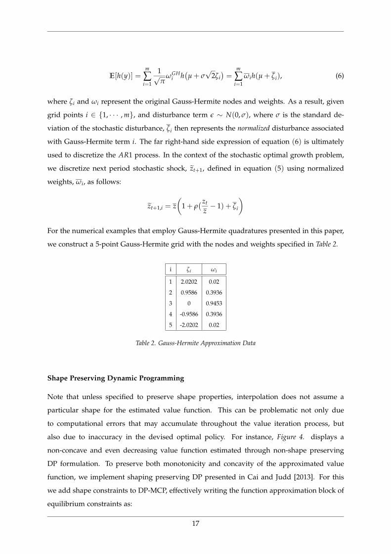
For the numerical examples that employ Gauss-Hermite quadratures presented in this paper,

we construct a 5-point Gauss-Hermite grid with the nodes and weights specified in Table 2.

i ζi ωi

1 2.0202 0.02

2 0.9586 0.3936

3 0 0.9453

4 -0.9586 0.3936

5 -2.0202 0.02

Table 2. Gauss-Hermite Approximation Data

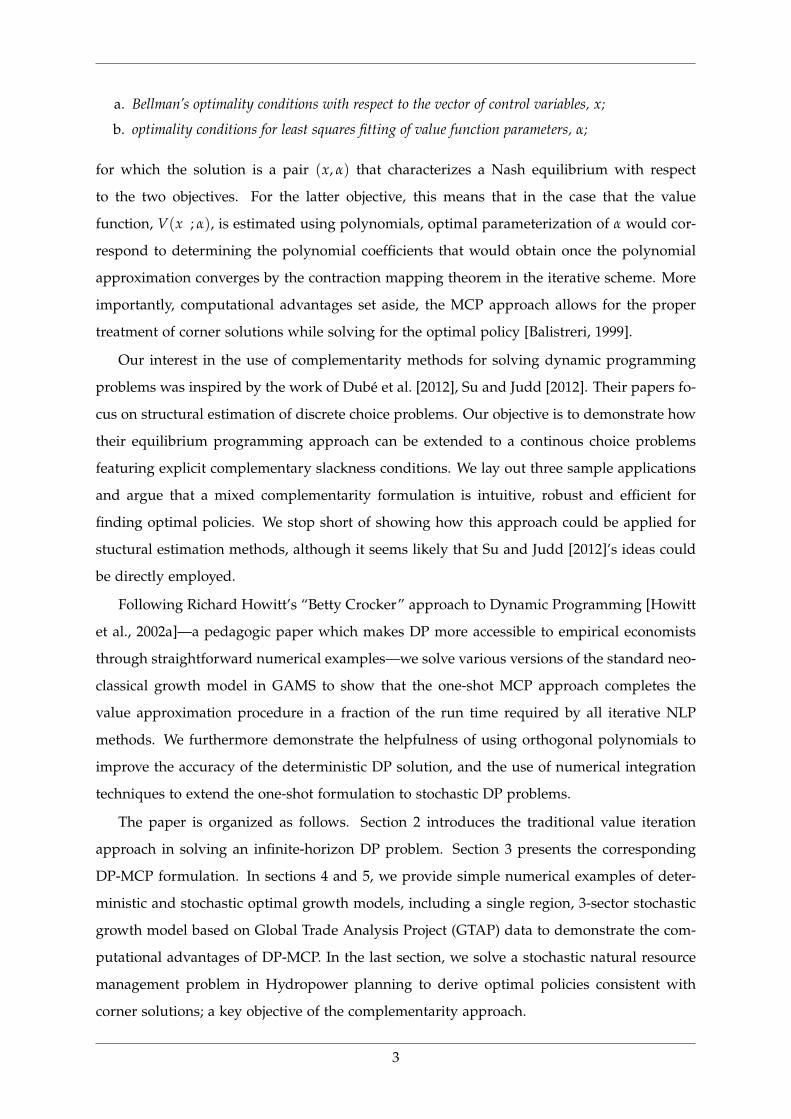
Shape Preserving Dynamic Programming

Note that unless specified to preserve shape properties, interpolation does not assume a

particular shape for the estimated value function. This can be problematic not only due

to computational errors that may accumulate throughout the value iteration process, but

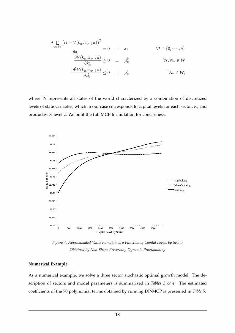
also due to inaccuracy in the devised optimal policy. For instance, Figure 4. displays a

non-concave and even decreasing value function estimated through non-shape preserving

DP formulation. To preserve both monotonicity and concavity of the approximated value

function, we implement shaping preserving DP presented in Cai and Judd [2013]. For this

we add shape constraints to DP-MCP, effectively writing the function approximation block of

equilibrium constraints as:

17

∂ ∑w∈W

(U −V(kw, zw ; α)

)2

∂αl= 0 ⊥ αl ∀l ∈ 0, · · · , 5

∂V(kw, zw ; α)

∂ksw

≥ 0 ⊥ µks

w ∀s, ∀w ∈W

∂2V(kw, zw ; α)

∂z2w

≤ 0 ⊥ µzw ∀w ∈W,

where W represents all states of the world characterized by a combination of discretized

levels of state variables, which in our case corresponds to capital levels for each sector, Ks and

productivity level z. We omit the full MCP formulation for conciseness.

Figure 4. Approximated Value Function as a Function of Capital Levels by Sector

Obtained by Non-Shape Preserving Dynamic Programming

Numerical Example

As a numerical example, we solve a three sector stochastic optimal growth model. The de-

scription of sectors and model parameters is summarized in Tables 3 & 4. The estimated

coefficients of the 70 polynomial terms obtained by running DP-MCP is presented in Table 5.

18

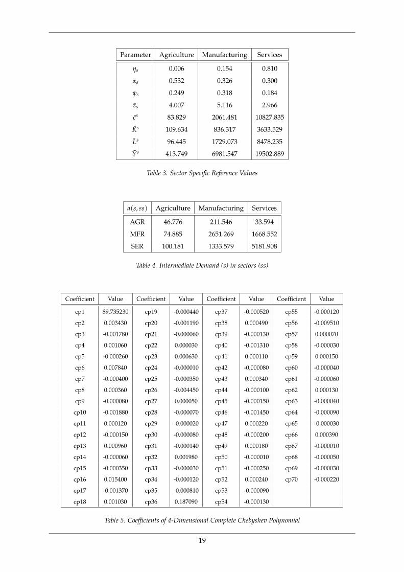
Parameter Agriculture Manufacturing Services

ηs 0.006 0.154 0.810

αs 0.532 0.326 0.300

ψs 0.249 0.318 0.184

zs 4.007 5.116 2.966

cs 83.829 2061.481 10827.835

Ks 109.634 836.317 3633.529

Ls 96.445 1729.073 8478.235

Ys 413.749 6981.547 19502.889

Table 3. Sector Specific Reference Values

a(s, ss) Agriculture Manufacturing Services

AGR 46.776 211.546 33.594

MFR 74.885 2651.269 1668.552

SER 100.181 1333.579 5181.908

Table 4. Intermediate Demand (s) in sectors (ss)

Coefficient Value Coefficient Value Coefficient Value Coefficient Value

cp1 89.735230 cp19 -0.000440 cp37 -0.000520 cp55 -0.000120

cp2 0.003430 cp20 -0.001190 cp38 0.000490 cp56 -0.009510

cp3 -0.001780 cp21 -0.000060 cp39 -0.000130 cp57 0.000070

cp4 0.001060 cp22 0.000030 cp40 -0.001310 cp58 -0.000030

cp5 -0.000260 cp23 0.000630 cp41 0.000110 cp59 0.000150

cp6 0.007840 cp24 -0.000010 cp42 -0.000080 cp60 -0.000040

cp7 -0.000400 cp25 -0.000350 cp43 0.000340 cp61 -0.000060

cp8 0.000360 cp26 -0.004450 cp44 -0.000100 cp62 0.000130

cp9 -0.000080 cp27 0.000050 cp45 -0.000150 cp63 -0.000040

cp10 -0.001880 cp28 -0.000070 cp46 -0.001450 cp64 -0.000090

cp11 0.000120 cp29 -0.000020 cp47 0.000220 cp65 -0.000030

cp12 -0.000150 cp30 -0.000080 cp48 -0.000200 cp66 0.000390

cp13 0.000960 cp31 -0.000140 cp49 0.000180 cp67 -0.000010

cp14 -0.000060 cp32 0.001980 cp50 -0.000010 cp68 -0.000050

cp15 -0.000350 cp33 -0.000030 cp51 -0.000250 cp69 -0.000030

cp16 0.015400 cp34 -0.000120 cp52 0.000240 cp70 -0.000220

cp17 -0.001370 cp35 -0.000810 cp53 -0.000090

cp18 0.001030 cp36 0.187090 cp54 -0.000130

Table 5. Coefficients of 4-Dimensional Complete Chebyshev Polynomial

19

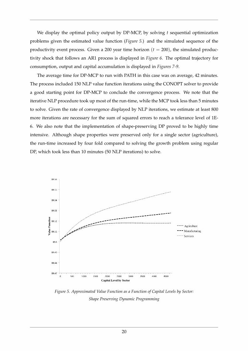
We display the optimal policy output by DP-MCP, by solving t sequential optimization

problems given the estimated value function (Figure 5.) and the simulated sequence of the

productivity event process. Given a 200 year time horizon (t = 200), the simulated produc-

tivity shock that follows an AR1 process is displayed in Figure 6. The optimal trajectory for

consumption, output and capital accumulation is displayed in Figures 7-9.

The average time for DP-MCP to run with PATH in this case was on average, 42 minutes.

The process included 150 NLP value function iterations using the CONOPT solver to provide

a good starting point for DP-MCP to conclude the convergence process. We note that the

iterative NLP procedure took up most of the run-time, while the MCP took less than 5 minutes

to solve. Given the rate of convergence displayed by NLP iterations, we estimate at least 800

more iterations are necessary for the sum of squared errors to reach a tolerance level of 1E-

6. We also note that the implementation of shape-preserving DP proved to be highly time

intensive. Although shape properties were preserved only for a single sector (agriculture),

the run-time increased by four fold compared to solving the growth problem using regular

DP, which took less than 10 minutes (50 NLP iterations) to solve.

Figure 5. Approximated Value Function as a Function of Capital Levels by Sector:

Shape Preserving Dynamic Programming

20

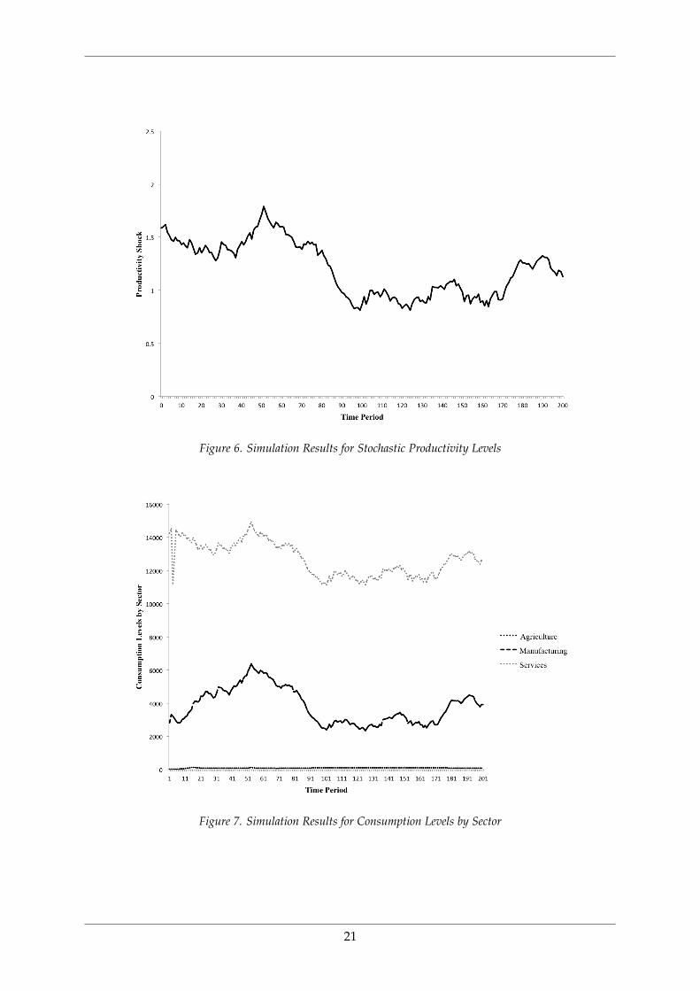
Figure 6. Simulation Results for Stochastic Productivity Levels

Figure 7. Simulation Results for Consumption Levels by Sector

21

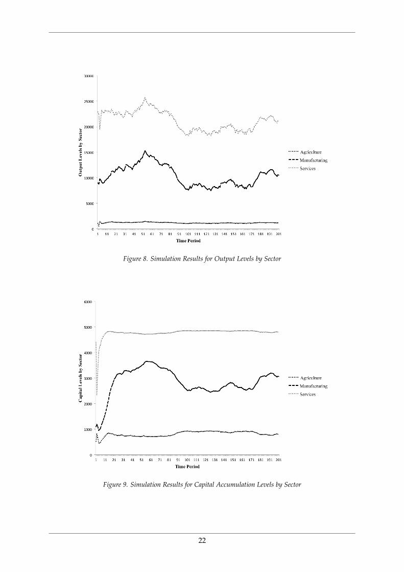
Figure 8. Simulation Results for Output Levels by Sector

Figure 9. Simulation Results for Capital Accumulation Levels by Sector

22

6. Stochastic Hydropower Planning

In this section we solve a mixed complementarity problem and illustrate DP-MCP’s accom-

modation of corner solutions. We also present quadrature methods that can be utilized in

the MCP formulation to solve stochastic dynamic programming models. The hydropower

planning problem is an annual model of a single aggregated reservoir with a monthly re-

lease schedule for hydropower generation. The present model is similar in dynamics to the

model of water management on the North Platte River in Nebraska presented in Howitt et al.

[2002a,b]. We begin with a brief overview of the model before describing algorithmic issues.

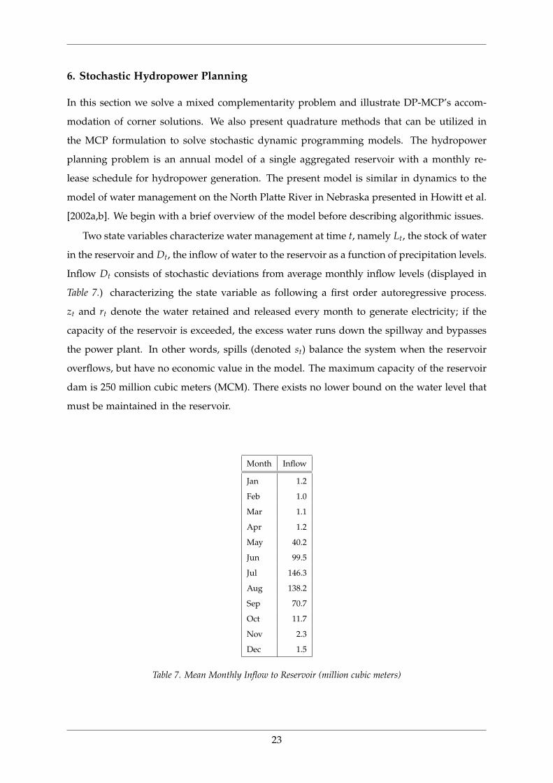
Two state variables characterize water management at time t, namely Lt, the stock of water

in the reservoir and Dt, the inflow of water to the reservoir as a function of precipitation levels.

Inflow Dt consists of stochastic deviations from average monthly inflow levels (displayed in

Table 7.) characterizing the state variable as following a first order autoregressive process.

zt and rt denote the water retained and released every month to generate electricity; if the

capacity of the reservoir is exceeded, the excess water runs down the spillway and bypasses

the power plant. In other words, spills (denoted st) balance the system when the reservoir

overflows, but have no economic value in the model. The maximum capacity of the reservoir

dam is 250 million cubic meters (MCM). There exists no lower bound on the water level that

must be maintained in the reservoir.

Month Inflow

Jan 1.2

Feb 1.0

Mar 1.1

Apr 1.2

May 40.2

Jun 99.5

Jul 146.3

Aug 138.2

Sep 70.7

Oct 11.7

Nov 2.3

Dec 1.5

Table 7. Mean Monthly Inflow to Reservoir (million cubic meters)

23

Lastly, monthly electricity generation must meet a fixed monthly demand of 140 megawatt

hours (MWH). In case electricity generated by hydropower does not meet demand, non-hydro

electricity generation is employed, incurring marginal cost equal to the market price of elec-

tricity. We begin by writing down the primal model.

Primal Equations

Water at the start of the month is either retained or released to generate electricity:

Lt ≥ zt + rt

Total generation of electricity through hydro (rt) and non-hydro (xt) sources must equal the

demand for electricity. Demand (denoted gt) is fixed in each month:

rt + xt = gt

The projected level of water at the start of the subsequent month (Lt+1) depends on how much

water is currently stored (zt), how much inflow is projected to occur (Dt+1) and how much

water will be spilled (st+1). Projected variable levels are represented using a tilde:

Lt+1 = zt + Dt+1 − st+1

The price of water in the subsequent month (pt+1) is imputed on the basis of the imputed

water price (value of water as a function of the state):

pt+1 = V(

Lt+1, Dt+1 ; α)

(7)

Lastly, inflow Dt follows an AR1 process such that the projected inflow Dt+1 is a function

of the mean monthly inflow Dt, the coefficient for rainfall persistence, ρ, the realized inflow

levels, Dt, and a normally distributed disturbance term ε ∼ N(0, σ) that represents stochastic

departures from the model.

Dt+1 = Dt+1

[1 + ρ

(Dt

Dt− 1)+ εt+1

](8)

The objective is to minimize non-hydro electricity generation while meeting the fixed demand

for electricity. This is presented in the following objective function:

24

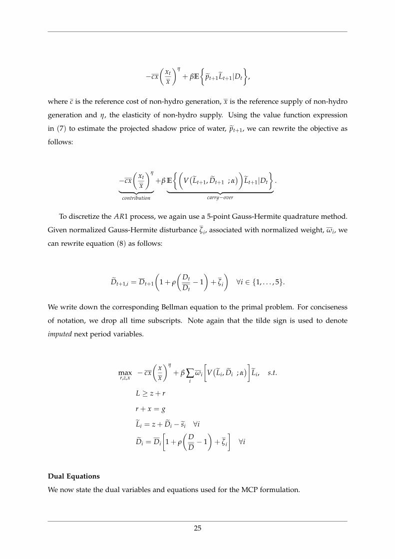
−cx(

xt

x

)η

+ βE

pt+1 Lt+1|Dt

,

where c is the reference cost of non-hydro generation, x is the reference supply of non-hydro

generation and η, the elasticity of non-hydro supply. Using the value function expression

in (7) to estimate the projected shadow price of water, pt+1, we can rewrite the objective as

follows:

−cx(

xt

x

)η

︸ ︷︷ ︸contribution

+β E

(V(

Lt+1, Dt+1 ; α))

Lt+1|Dt

︸ ︷︷ ︸

carry−over

.

To discretize the AR1 process, we again use a 5-point Gauss-Hermite quadrature method.

Given normalized Gauss-Hermite disturbance ζ i, associated with normalized weight, ωi, we

can rewrite equation (8) as follows:

Dt+1,i = Dt+1

(1 + ρ

(Dt

Dt− 1)+ ζ i

)∀i ∈ 1, . . . , 5.

We write down the corresponding Bellman equation to the primal problem. For conciseness

of notation, we drop all time subscripts. Note again that the tilde sign is used to denote

imputed next period variables.

maxr,z,x

− cx(

xx

)η

+ β ∑i

ωi

[V(

Li, Di ; α)]

Li, s.t.

L ≥ z + r

r + x = g

Li = z + Di − si ∀i

Di = Di

[1 + ρ

(DD− 1)+ ζ i

]∀i

Dual Equations

We now state the dual variables and equations used for the MCP formulation.

25

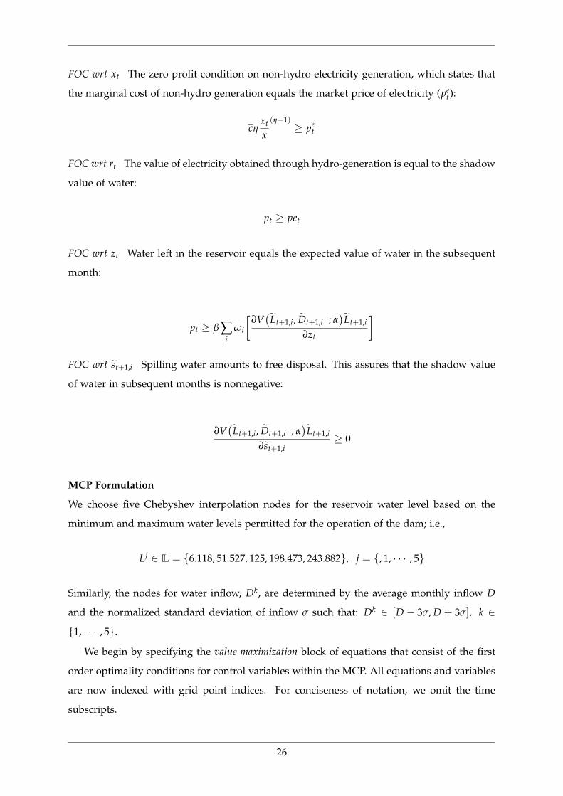
FOC wrt xt The zero profit condition on non-hydro electricity generation, which states that

the marginal cost of non-hydro generation equals the market price of electricity (pet):

cηxt

x

(η−1)≥ pe

t

FOC wrt rt The value of electricity obtained through hydro-generation is equal to the shadow

value of water:

pt ≥ pet

FOC wrt zt Water left in the reservoir equals the expected value of water in the subsequent

month:

pt ≥ β ∑i

ωi

[∂V(

Lt+1,i, Dt+1,i ; α)

Lt+1,i

∂zt

]

FOC wrt st+1,i Spilling water amounts to free disposal. This assures that the shadow value

of water in subsequent months is nonnegative:

∂V(

Lt+1,i, Dt+1,i ; α)

Lt+1,i

∂st+1,i≥ 0

MCP Formulation

We choose five Chebyshev interpolation nodes for the reservoir water level based on the

minimum and maximum water levels permitted for the operation of the dam; i.e.,

Lj ∈ L = 6.118, 51.527, 125, 198.473, 243.882, j = , 1, · · · , 5

Similarly, the nodes for water inflow, Dk, are determined by the average monthly inflow D

and the normalized standard deviation of inflow σ such that: Dk ∈ [D − 3σ, D + 3σ], k ∈

1, · · · , 5.

We begin by specifying the value maximization block of equations that consist of the first

order optimality conditions for control variables within the MCP. All equations and variables

are now indexed with grid point indices. For conciseness of notation, we omit the time

subscripts.

26

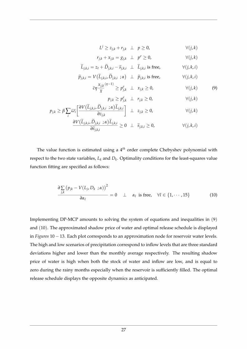
Lj ≥ zj,k + rj,k ⊥ p ≥ 0, ∀(j, k)

rj,k + xj,k = gj,k ⊥ pe ≥ 0, ∀(j, k)

Lj,k,i = zt + Dj,k,i − sj,k,i ⊥ Lj,k,i is free, ∀(j, k, i)

pj,k,i = V(

Lj,k,i, Dj,k,i ; α)⊥ pj,k,i is free, ∀(j, k, i)

cηxj,k

x

(η−1)≥ pe

j,k ⊥ xj,k ≥ 0, ∀(j, k) (9)

pj,k ≥ pej,k ⊥ rj,k ≥ 0, ∀(j, k)

pj,k ≥ β ∑i

ωi

[∂V(

Lj,k,i, Dj,k,i ; α)

Lj,k,i

∂zj,k

]⊥ zj,k ≥ 0, ∀(j, k)

∂V(

Lj,k,i, Dj,k,i ; α)

Lj,k,i

∂sj,k,i≥ 0 ⊥ sj,k,i ≥ 0, ∀(j, k, i)

The value function is estimated using a 4th order complete Chebyshev polynomial with

respect to the two state variables, Lk and Dk. Optimality conditions for the least-squares value

function fitting are specified as follows:

∂ ∑j,k

(pjk −V(Lj, Dk ; α)

)2

∂αl= 0 ⊥ αl is free, ∀l ∈ 1, · · · , 15 (10)

Implementing DP-MCP amounts to solving the system of equations and inequalities in (9)

and (10). The approximated shadow price of water and optimal release schedule is displayed

in Figures 10− 13. Each plot corresponds to an approximation node for reservoir water levels.

The high and low scenarios of precipitation correspond to inflow levels that are three standard

deviations higher and lower than the monthly average respectively. The resulting shadow

price of water is high when both the stock of water and inflow are low, and is equal to

zero during the rainy months especially when the reservoir is sufficiently filled. The optimal

release schedule displays the opposite dynamics as anticipated.

27

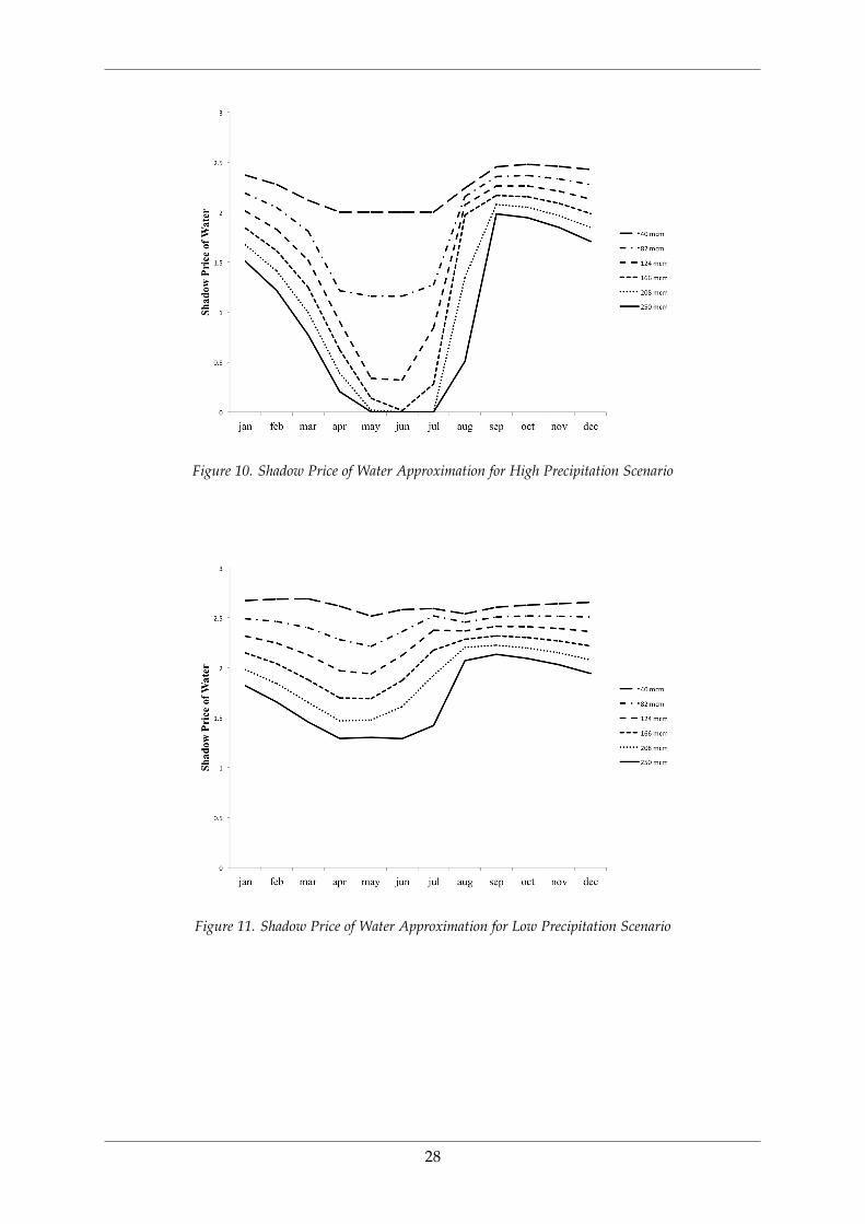
Figure 10. Shadow Price of Water Approximation for High Precipitation Scenario

Figure 11. Shadow Price of Water Approximation for Low Precipitation Scenario

28

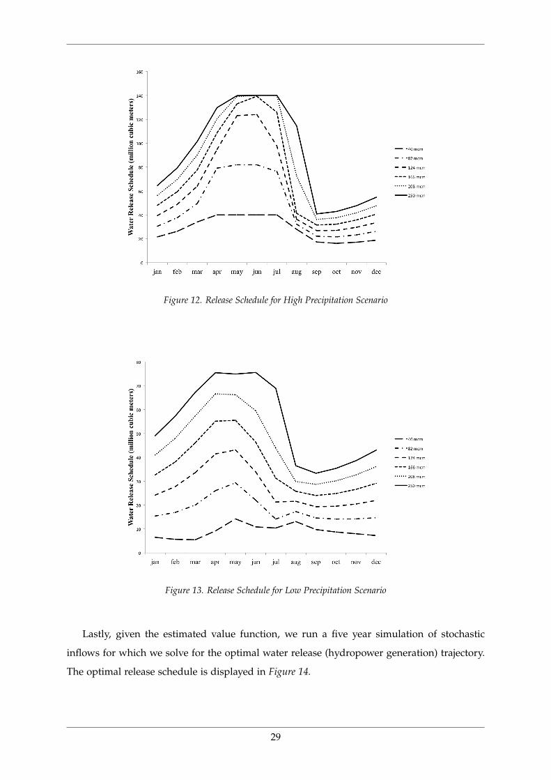
Figure 12. Release Schedule for High Precipitation Scenario

Figure 13. Release Schedule for Low Precipitation Scenario

Lastly, given the estimated value function, we run a five year simulation of stochastic

inflows for which we solve for the optimal water release (hydropower generation) trajectory.

The optimal release schedule is displayed in Figure 14.

29

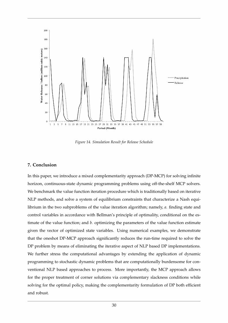
Figure 14. Simulation Result for Release Schedule

7. Conclusion

In this paper, we introduce a mixed complementarity approach (DP-MCP) for solving infinite

horizon, continuous-state dynamic programming problems using off-the-shelf MCP solvers.

We benchmark the value function iteration procedure which is traditionally based on iterative

NLP methods, and solve a system of equilibrium constraints that characterize a Nash equi-

librium in the two subproblems of the value iteration algorithm; namely, a. finding state and

control variables in accordance with Bellman’s principle of optimality, conditional on the es-

timate of the value function; and b. optimizing the parameters of the value function estimate

given the vector of optimized state variables. Using numerical examples, we demonstrate

that the oneshot DP-MCP approach significantly reduces the run-time required to solve the

DP problem by means of eliminating the iterative aspect of NLP based DP implementations.

We further stress the computational advantages by extending the application of dynamic

programming to stochastic dynamic problems that are computationally burdensome for con-

ventional NLP based approaches to process. More importantly, the MCP approach allows

for the proper treatment of corner solutions via complementary slackness conditions while

solving for the optimal policy, making the complementarity formulation of DP both efficient

and robust.

30

REFERENCES REFERENCES

References

Extensions of GAMS for complementarity problems arising in applied economics. Journal ofEconomic Dynamics and Control, 19(8):1299–1324, 1995.

S Boragan Aruoba and Jesús Fernández-Villaverde. A comparison of programming languagesin economics. Technical report, National Bureau of Economic Research, 2014.

Edward J Balistreri. Playing the bertrand game in the corner: A mixed complementarityformulation with endogenous entry. 1999.

William J Baumol. Activity analysis in one lesson. The American Economic Review, 48(5):837–873, 1958.

R Bellman. Dynamic programming. rand corporation research study. Princeton UniversityPress, 1957b. ISBN, 1050546524:3, 1957.

Paolo Brandimarte. Handbook in Monte Carlo simulation: applications in financial engineering, riskmanagement, and economics. John Wiley & Sons, 2014.

William A Brock and Leonard J Mirman. Optimal economic growth and uncertainty: thediscounted case. Journal of Economic Theory, 4(3):479–513, 1972.

Yongyang Cai and Kenneth L Judd. Shape-preserving dynamic programming. MathematicalMethods of Operations Research, 77(3):407–421, 2013.

Yongyang Cai and Kenneth L Judd. Dynamic programming with hermite approximation.Mathematical Methods of Operations Research, 81(3):245–267, 2015.

Wonjun Chang. Assessing the uncertainty effects of near-term climate policy recommenda-tions: A stochastic programming approach. University of Wisconsin-Davis, 2016.

Steven P Dirkse and Michael C Ferris. The PATH solver: a nommonotone stabilization schemefor mixed complementarity problems. Optimization Methods and Software, 5(2):123–156, 1995.

Jean-Pierre Dubé, Jeremy T Fox, and Che-Lin Su. Improving the numerical performanceof static and dynamic aggregate discrete choice random coefficients demand estimation.Econometrica, 80(5):2231–2267, 2012.

Michael C Ferris and Todd S Munson. Complementarity problems in gams and the PATHsolver. Journal of Economic Dynamics and Control, 24(2):165–188, 2000.

Michael C Ferris and Krung Sinapiromsaran. Formulating and solving nonlinear programsas mixed complementarity problems. In Optimization, pages 132–148. Springer, 2000.

Michael C Ferris, Steven P Dirkse, Jan-H Jagla, and Alexander Meeraus. An extended math-ematical programming framework. Computers & Chemical Engineering, 33(12):1973–1982,2009.

Richard Howitt, Siwa Msangi, Arnaud Reynaud, and Keith Knapp. Using polynomial ap-proximations to solve stochastic dynamic programming problems: Or a ’betty crocker’approach to sdp. University of California, Davis, 2002a.

Richard E Howitt, Arnaud Reynaud, Siwa Msangi, Keith C Knapp, et al. Calibrated stochasticdynamic models for resource management. In The 2nd World Congress of Environmental andResource Economists, volume 2427, 2002b.

Kenneth L Judd. Numerical methods in economics. MIT press, 1998.

31

REFERENCES REFERENCES

Kenneth L Judd, Lilia Maliar, Serguei Maliar, and Rafael Valero. Smolyak method for solvingdynamic economic models: Lagrange interpolation, anisotropic grid and adaptive domain.Journal of Economic Dynamics and Control, 44:92–123, 2014.

Karen A Kopecky. Function approximation. University of Western Ontario Lectures Notes ECO613/614 Fall 2007, 2007.

Thomas S Lontzek, Yongyang Cai, and Kenneth L Judd. Tipping points in a dynamic stochas-tic iam. 2012.

Lilia Maliar and Serguei Maliar. Merging simulation and projection approaches to solvehigh-dimensional problems with an application to a new keynesian model. QuantitativeEconomics, 6(1):1–47, 2015.

Rodolfo E Manuelli and Thomas J Sargent. Exercises in dynamic macroeconomic theory. HarvardUniversity Press, 2009.

John C Mason and David C Handscomb. Chebyshev polynomials. CRC Press, 2002.

Beresford N Parlett, H Simon, and LM Stringer. On estimating the largest eigenvalue withthe lanczos algorithm. Mathematics of computation, 38(157):153–165, 1982.

Warren B Powell. Approximate Dynamic Programming: Solving the Curses of Dimensionality,volume 842. John Wiley & Sons, 2011.

John Rust. Numerical dynamic programming in economics. Handbook of computational eco-nomics, 1:619–729, 1996.

Yousef Saad. On the rates of convergence of the lanczos and the block-lanczos methods. SIAMJournal on Numerical Analysis, 17(5):687–706, 1980.

Thomas Sargent and John Stachurski. Quantitative economics with python. Technical report,Technical report, Lecture Notes, 2015.

Herbert Scarf et al. On the computation of equilibrium prices. Number 232. Cowles Foundationfor Research in Economics at Yale University, 1967.

Nancy L Stokey and Robert E with Edward C. Prescott Lucas Jr. Recursive methods in eco-nomic dynamics, 1989.

Che-Lin Su and Kenneth L Judd. Constrained optimization approaches to estimation of struc-tural models. Econometrica, 80(5):2213–2230, 2012.

George Tauchen. Finite state markov-chain approximations to univariate and vector autore-gressions. Economics letters, 20(2):177–181, 1986.

Stephen Wright and Jorge Nocedal. Numerical optimization. Springer Science, 35:67–68, 1999.

32

REFERENCES REFERENCES

Appendix: GAMS Code

1. Brock-Mirman Stochastic Growth Model

1 $title Stochastic Brock−Mirman Growth Model Using Chebyshev Polynomial Approximation:

3 ∗ This program includes both DP−NLP and DP−MCP formulations

5 Sets s State variables /cap,phi/,6 ik Nodes for capital at which value function is evaluated /1∗5/,7 ip Nodes for productivity /1∗5/,8 ic Dimension of Chebyshev polynomial /1∗5/,9 iter Dynamic programming iterations /1 ∗ 2000/;

11 alias (ik,jk)12 alias (ip,jp)13 alias (ic,jc)14 alias (s,ss)

16 Parameters17 eta Elasticity of the marginal utility of consumption /0.95/,18 beta Utility discount factor /0.9888/,19 alpha Capital value share /0.333/,20 pi /3.141593/;

23 ∗ Parameters to define CS Polynomial terms24 ∗ Defined for both capital (K) and productivity (p)

26 Parameters27 arg_k, arg_p Argument of cosine weighting function,28 x_k, x_p Node value for the state variable on the unit interval,29 lo_k, lo_p Lowerbound on stock variable,30 up_k, up_p Upperbound on stock variable,31 csbar(ic) Chebyshev polynomial terms,32 cap(ik) Stock level value at node for grid point calculation,33 phi(ip) Stock level value at node for grid point calculation;

35 Parameters36 sigma Normalized standard deviation of phi /0.1/,37 p_mean Mean value of productivity phi /5/,38 p_std Standard deviation of phi;

41 ∗ Set lower and upper bound on state variables

43 p_std = sigma ∗ p_mean;44 lo_p = p_mean − 3∗p_std;45 up_p = p_mean + 3∗p_std;

47 lo_k = 0;48 up_k = 5;

50 ∗ Define basis for chebyshev polynomial expansion

52 ∗ Capital

54 arg_k(ik) = ((2∗ord(ik)−1)∗pi)/(2∗card(ik));55 x_k(ik) = cos(arg_k(ik));56 cap(ik) = (lo_k+up_k+(up_k−lo_k)∗x_k(ik))/2;

58 ∗ Productivity

60 arg_p(ip) = ((2∗ord(ip)−1)∗pi)/(2∗card(ip));61 x_p(ip) = cos(arg_p(ip));62 phi(ip) = (lo_p+up_p+(up_p−lo_p)∗x_p(ip))/2;

64 ∗ Define terms included in Chebyshev polynomial basis functions in the form:65 ∗ cc(ic) ∗ X∗∗ce(ic)66 ∗ where cc(ic) is the coefficient, X is the state and ce(ic), the exponent67 ∗ for each component of Chebyshev basis functions.

33

REFERENCES REFERENCES

69 $include chebyshevp_term_define

71 ∗−−−−−−−−−−−−−−−−−−−−−−−−−−−−−−−−−−−−−−−−−−−−−−−−−−−−−−−−−−−−−−−−−−−−−−−−−−−−−−−−−−−−−−72 ∗ Present value function based on Chebyshev polynomial terms73 ∗−−−−−−−−−−−−−−−−−−−−−−−−−−−−−−−−−−−−−−−−−−−−−−−−−−−−−−−−−−−−−−−−−−−−−−−−−−−−−−−−−−−−−−

75 ∗ Least−squares estimation76 $macro PVL(kbar,phibar,ik,ip) (sum(cp, A(cp) ∗ \77 sum(ic,kbar(ik,ic)$(ic.val eq cpe("cap",cp))) ∗ \78 sum(ic,phibar(ip,ic)$(ic.val eq cpe("phi",cp)))))

80 ∗ Value function computation81 $macro PV(KCS,phitcs,ik,ip,jp) (sum(cp, A(cp) ∗ \82 sum(ic,KCS(ik,ip,ic)$(ic.val eq cpe("cap",cp))) ∗ \83 sum(ic,phitcs(jp,ic)$(ic.val eq cpe("phi",cp)))))

85 ∗ Normalized value of K used in Chebyshev Polynomials86 $macro KN(ik,ip) ((K(ik,ip)−(lo_k+up_k)/2)/((up_k−lo_k)/2))

89 ∗−−−−−−−−−−−−−−−−−−−−−−−−−−−−−−−−−−−−−−−−−−−−−−−−−−−−−−−−−−−−−−−−−−−−−−−−−−−−−−−−−−−−−−90 ∗ Transition Matrix91 ∗−−−−−−−−−−−−−−−−−−−−−−−−−−−−−−−−−−−−−−−−−−−−−−−−−−−−−−−−−−−−−−−−−−−−−−−−−−−−−−−−−−−−−−

93 Table tmatrix(ip,jp)

96 1 2 3 4 597 1 0.9727 0.0273 0 0 098 2 0.0041 0.9806 0.0153 0 099 3 0 0.0082 0.9837 0.0082 0100 4 0 0 0.0153 0.9806 0.0041101 5 0 0 0 0.0273 0.9727;

104 Parameters105 phit Grid point values of approximated phi,106 phitn Normalized grid point values of projected phi,107 phitcs CS Polynomial terms used for value approximation;

110 ∗ stochasticity

112 phit(ip) = phi(ip);113 phitn(ip) = ((phit(ip)−(lo_p+up_p)/2)/((up_p−lo_p)/2));

115 ∗−−−−−−−−−−−−−−−−−−−−−−−−−−−−−−−−−−−−−−−−−−−−−−−−−−−−−−−−−−−−−−−−−−−−−−−−−−−−−−−−−−−−−−116 ∗ Apply Chebyshev polynomial algorithm on productivity117 ∗−−−−−−−−−−−−−−−−−−−−−−−−−−−−−−−−−−−−−−−−−−−−−−−−−−−−−−−−−−−−−−−−−−−−−−−−−−−−−−−−−−−−−−

119 phitcs(ip,ic) = sum((pt,pst), cc(ic,pt,pst)$csp(ic,pt,pst)∗120 power(phitn(ip),ce(ic,pt,pst)$csp(ic,pt,pst)));

123 ∗−−−−−−−−−−−−−−−−−−−−−−−−−−−−−−−−−−−−−−−−−−−−−−−−−−−−−−−−−−−−−−−−−−−−−−−−−−−−−−−−−−−−−−124 ∗ Define Bellman Equation125 ∗−−−−−−−−−−−−−−−−−−−−−−−−−−−−−−−−−−−−−−−−−−−−−−−−−−−−−−−−−−−−−−−−−−−−−−−−−−−−−−−−−−−−−−

127 Variables128 OBJ Objective129 C(ik,ip) Consumption,130 K(ik,ip) Subsequent period capital stock,131 U(ik,ip) Nodal approximations of utility,132 A(cp) Terms in the value function approximation,133 KCS(ik,ip,ic) Chebyshev polynomial terms (ic) for capital,134 P(ik,ip) Shadow price of capital;

136 Equations137 utility Present value benefit function,138 market Market for current output,139 objdef Least squares objective,140 k_csdef Chebyshev polynomial terms for capital,141 foca First order condition for coefficient A,

34

REFERENCES REFERENCES

142 copt First order condition for consumption,143 kopt First order condition for capital,144 udef Defines nodal utility;

146 utility.. OBJ =e= sum((ik,ip), 1/(1−eta) ∗ C(ik,ip)∗∗(1−eta) +147 beta ∗ sum(jp, tmatrix(ip,jp) ∗ PV(KCS,phitcs,ik,ip,jp)));

150 market(ik,ip).. C(ik,ip) + K(ik,ip) =e= phi(ip) ∗ cap(ik)∗∗alpha;

152 objdef.. OBJ =e= sum((ik,ip), sqr(PVL(kbar,phibar,ik,ip) − U(ik,ip)));

154 k_csdef(ik,ip,ic)..155 KCS(ik,ip,ic) =e= sum((pt,pst), cc(ic,pt,pst)$csp(ic,pt,pst)∗156 power(KN(ik,ip),ce(ic,pt,pst)$csp(ic,pt,pst)));

158 foca(cpp).. sum((ik,ip), 2 ∗159 (PVL(kbar,phibar,ik,ip) − U(ik,ip)) ∗160 sum(ic,kbar(ik,ic)$(ic.val eq cpe("cap",cpp))) ∗161 sum(ic,phibar(ip,ic)$(ic.val eq cpe("phi",cpp)))162 ) =e= 0;

164 copt(ik,ip).. P(ik,ip) =g= C(ik,ip)∗∗(−eta);

166 kopt(ik,ip).. P(ik,ip) =g=167 beta/((up_k − lo_k)/2) ∗168 sum(jp, tmatrix(ip,jp) ∗169 sum(cp, A(cp) ∗ sum(ic, phitcs(jp,ic)$(ic.val eq cpe("phi",cp))) ∗170 sum(ic,171 sum((pt,pst),172 (cc(ic,pt,pst)$(csp(ic,pt,pst)) ∗173 ce(ic,pt,pst)$(csp(ic,pt,pst)) ∗174 power(KN(ik,ip),ce(ic,pt,pst)−1))$(ce(ic,pt,pst) ge 1)175 )$(ic.val eq cpe("cap",cp))176 )177 )178 );

180 udef(ik,ip).. U(ik,ip) =e=181 1/(1−eta) ∗ C(ik,ip)∗∗(1−eta) +182 beta ∗ sum(jp, tmatrix(ip,jp) ∗ PV(KCS,phitcs,ik,ip,jp));

184 model bellman /utility,market,k_csdef/;185 model lsqr /objdef/;186 model oneshot_mcp /foca.A, copt.C, kopt.K, market.P, udef.U, k_csdef.KCS/;

188 ∗−−−−−−−−−−−−−−−−−−−−−−−−−−−−−−−−−−−−−−−−−−−−−−−−−−−−−−−−−−−−−−−−−−−−−−−−−−−−−−−−−−−−−−189 ∗ Initialization190 ∗−−−−−−−−−−−−−−−−−−−−−−−−−−−−−−−−−−−−−−−−−−−−−−−−−−−−−−−−−−−−−−−−−−−−−−−−−−−−−−−−−−−−−−

192 C.LO(ik,ip) = 1e−6;193 K.LO(ik,ip) = 0;194 A.L(cp) = 1;

196 ∗−−−−−−−−−−−−−−−−−−−−−−−−−−−−−−−−−−−−−−−−−−−−−−−−−−−−−−−−−−−−−−−−−−−−−−−−−−−−−−−−−−−−−−197 ∗ Value Iteration198 ∗−−−−−−−−−−−−−−−−−−−−−−−−−−−−−−−−−−−−−−−−−−−−−−−−−−−−−−−−−−−−−−−−−−−−−−−−−−−−−−−−−−−−−−

200 ∗ Parmeters for value function iteration

202 Parameters203 dev Current deviation coef /1/,204 itlog Iteration log;

206 ∗ Initial value:

208 U.FX(ik,ip) = 1;

210 file ktitle; ktitle.lw=0;

212 bellman.solvelink = 2;213 loop(iter$round(dev,10),

35

REFERENCES REFERENCES

215 itlog(iter,cp) = A.L(cp);

217 A.LO(cp) = −INF; A.UP(cp) = +INF;

219 solve lsqr using nlp minimzing OBJ;

221 dev = sum(cp,sqr(A.L(cp)−itlog(iter,cp)));

223 itlog(iter,"dev") = dev;

225 A.FX(cp) = A.L(cp);

227 solve bellman using nlp max obj;228 abort$(bellman.solvestat<>1 and bellman.modelstat>2) "Bellman does not solve.";229 U.FX(ik,ip) = 1/(1−eta) ∗ C.L(ik,ip)∗∗(1−eta) + beta ∗230 sum(jp, tmatrix(ip,jp) ∗231 sum(cp, A.L(cp) ∗232 sum(ic, KCS.L(ik,ip,ic)$(ic.val eq cpe("cap",cp))) ∗233 sum(ic,phitcs(jp,ic)$(ic.val eq cpe("phi",cp)))234 )235 );236 put ktitle;237 put_utility ’title’ /’Iter: ’,iter.tl,’ Deviation = ’,dev;

239 );

241 A.LO(cp) = −inf;242 A.UP(cp) = +inf;243 U.UP(ik,ip) = +inf;244 U.LO(ik,ip) = −inf;245 P.L(ik,ip) = market.m(ik,ip);

247 solve oneshot_mcp using mcp;248 display K.L, U.L, A.L, KCS.L;

36

REFERENCES REFERENCES

2. Hydropower Planning Model

1 $title NLP−MCP Hybrid Formulation of Hydropower Planning Model:

3 ∗ GAMS code for 2nd order polynomial estimation

5 ∗ Number of reservior level nodes:

7 $if not set nkl $set nkl 5

9 ∗ Number of precipitation level nodes:

11 $if not set nkp $set nkp 3

13 Set m Months /jan, feb, mar, apr, may, jun,14 jul, aug, sep, oct, nov, dec /;

17 Parameters inflow(m) Mean inflow (million m3) /18 jan 1.2,19 feb 1.0,20 mar 1.1,21 apr 1.2,22 may 40.2,23 jun 99.5,24 jul 146.3,25 aug 138.2,26 sep 70.7,27 oct 11.7,28 nov 2.3,29 dec 1.5 /;

31 ∗ Set maximum capcity of reservoir

33 $if not set rmax $set rmax 140

35 Parameters36 lmax Maximum water level the dam can store (million m3) /250/,37 lmin Minimum water level that must be maintained (million m3) /0/,38 rmax Maximum amount that can be released per month (m. m3) /%rmax%/,39 g(m) Monthly demand (fixed),40 cref Reference cost /1/,41 eta Elasticity of non−hydro supply /2/,42 xref Reference non−hydro supply /100/;

44 g(m) = 140;

46 Set kl Water level grid points /0∗%nkl%/;

48 Parameters49 L(kl,m) Water levels at grid points,50 theta(∗) Parameter defining convex combinations;

52 ∗ Water level state variable uniformly distributed53 ∗ between the min and max level:

55 theta(kl) = (ord(kl)−1)/(card(kl)−1);56 L(kl,m) = lmin ∗ (1−theta(kl)) + lmax ∗ theta(kl);

58 Set kp Precipitation grid points /0∗%nkp%/;

60 Parameters61 dfac Monthly discount factor (6% per year) /0.99/62 rhod Rainfall persistence (highly persistent) /0.9/63 sigma Normalized standard deviation of inflow /0.1/,64 d_mean Mean value of d65 d_std Standard deviation of d66 d_low Low value of d on the grid,67 d_high High value of d on the grid,68 d(kp,m) Grid point values of d;

71 ∗ AR(1) mean:

37

REFERENCES REFERENCES

73 d_mean(m) = inflow(m);

75 ∗ AR(1) std. dev.:

77 d_std(m) = sigma ∗ d_mean(m) /sqrt((1−rhod∗∗2));78 d_low(m) = d_mean(m) − 3∗d_std(m);79 d_high(m) = d_mean(m) + 3∗d_std(m);

81 ∗ Set up the Gauss−Hermite grid:

83 Set i Gaussian−Hermite grid points /1∗5/

86 ∗ Implementing GH:87 ∗ 1. Get n nodes and n weights from a computer program

89 Table ghdata(i,∗) Tabulated Gaussian−Hermite approximation points

91 zeta omega92 1 2.0202 0.0293 2 0.9586 0.393694 3 0 0.945395 4 −0.9586 0.393696 5 −2.0202 0.02;

98 Parameter99 omega(i) Normalized GH weights,100 zeta(m,i) Normalized GH nodes,101 dt(kp,m,i) Grid point values of dt;

103 ∗ Take expectation of function value:104 ∗ omega(i) ∗ h(zeta)

106 omega(i) = ghdata(i,"omega")/sqrt(3.141592);107 zeta(m,i) = sigma∗sqrt(2)∗ghdata(i,"zeta");

109 ∗ discretize precipitation levels

111 theta(kp) = (ord(kp)−1)/(card(kp)−1);112 d(kp,m) = d_low(m) ∗ (1−theta(kp)) + d_high(m) ∗ theta(kp);

114 ∗ Rainfall in realization i following month m is115 ∗ defined relative to the mean rainfall in month m++1.116 ∗ zeta is normally distributed:

118 dt(kp,m++1,i) = max(0, d_mean(m++1) ∗ (1 + rhod ∗ (d(kp,m)/d_mean(m)−1) + zeta(m++1,i)));

120 Set ja /0∗2/ Set index for coefficients: L,121 jb /0∗2/ Set index for coefficients: d,122 k(kl,kp) State of the world;

124 k(kl,kp) = yes;

126 alias (ja,ja_), (jb,jb_);

128 ∗ First order taylor linear approximation of the optimal129 ∗ present value of month m with reservoir level L and precipitation d:130 ∗ searching for taylor approximation coefficients

132 $macro PV(m,L,d) (sum(ja_,A(ja_,m)∗power(L,ja_.val))+sum(jb_,B(jb_,m)∗power(d,jb_.val)))

134 Variables135 P(kl,kp,m) Current estimate of the shadow price of water,136 A(ja,m) Polynomial approximation terms for L,137 B(jb,m) Polynomial approximation terms for d,138 PE(kl,kp,m) Shadow price of electricity,139 X(kl,kp,m) Non−hydro generation,140 Z(kl,kp,m) Water retained,141 R(kl,kp,m) Water released to generate electricity,142 S(kl,kp,m,i) Water spilled without generating electricity,143 PT(kl,kp,m,i) Projected shadow price,144 MU(kl,kp,m,i) Shadow price on upper bound constraint,

38

REFERENCES REFERENCES

145 LT(kl,kp,m,i) Projected level;

147 Free Variable148 OBJ NLP Objective;

150 Nonnegative Variables Z,R,S;

152 Equations objdef, supply, demand, ptdef, supplyt, upper, lsqrdef;

154 ∗ NLP Objective Definition

156 objdef.. OBJ =e= sum((k(kl,kp),m),

158 ∗ Discounted expected value of subsequent state:

160 dfac ∗ sum(i, omega(i) ∗

162 ∗ Value of water delivered in the subsequent month:

164 PT(k,m++1,i) ∗ LT(k,m++1,i))

166 ∗ Cost of using non−hydro generation this month:

168 − cref ∗ xref ∗ (X(k,m)/xref)∗∗(eta) );

171 ∗ Water at the start of the month is either retained or released to172 ∗ generate electricity:

174 supply(k(kl,kp),m).. L(kl,m) =g= Z(k,m) + R(k,m);

176 ∗ Total generation equals that provided by hydro and non−hydro177 ∗ sources. Demand is fixed in each month:

179 demand(k(kl,kp),m).. g(m) =e= R(k,m) + X(k,m);

181 ∗ The level of water at the start of month m depends on how much water182 ∗ was stored the previous month (Z), how much inflow occurred (dt) and183 ∗ how much water was spilled (S):

185 supplyt(k(kl,kp),m,i).. LT(k,m,i) =e= Z(k,m−−1) + dt(kp,m,i) − S(k,m,i);

187 ∗ The price of water in the subsequent month is imputed on the basis of188 ∗ the imputed water price on the nodes along with the shadow prices of189 ∗ the upper and lower bounds on capacity:

191 ptdef(k(kl,kp),m,i).. PT(k,m,i) =e= PV(m, LT(k,m,i), dt(kp,m,i));

193 ∗ Least−squares estimation of shadow price of water

195 lsqrdef.. OBJ =E= sum((k(kl,kp),m), sqr(PV(m,L(kl,m),d(kp,m)) − p(k,m)));

197 Equations foc_a(ja,m) First order condition for a (MCP formlation)198 foc_b(jb,m) First order condition for b (MCP formulation);

200 foc_a(ja,m).. −sum(k(kl,kp),(P(k,m)−PV(m,L(kl,m),d(kp,m))) ∗ power(L(kl,m),ja.val)) =e= 0;

202 foc_b(jb,m).. −sum(k(kl,kp),(P(k,m)−PV(m,L(kl,m),d(kp,m))) ∗ power(d(kp,m),jb.val)) =e= 0;

204 ∗ Dual equations for MCP

206 Equations xopt, ropt, zopt, sopt;

208 ∗ Marginal cost of non−hydro generation equals market price of209 ∗ electricity:

211 xopt(k(kl,kp),m).. cref ∗ eta ∗ (X(k,m)/xref)∗∗(eta−1) =g= PE(k,m);

213 ∗ Hydro generation is equalized with the shadow value of water:

215 ropt(k(kl,kp),m).. P(k,m) =g= PE(k,m);

217 ∗ Risk neutral: water left in the reservior equals the expected

39

REFERENCES REFERENCES

218 ∗ value of water in the subsequent month:

220 zopt(k(kl,kp),m).. P(k,m) =g= dfac ∗ sum(i, omega(i) ∗221 (PT(k,m++1,i) +222 LT(k,m++1,i)∗(A("1",m++1) +223 2∗A("2",m++1)∗LT(k,m++1,i)) ));

225 ∗ Spilling water amounts to free disposal. This assures that226 ∗ the shadow value of water in subsequent months is nonnegative:

228 sopt(k(kl,kp),m,i).. dfac ∗ omega(i) ∗ (PT(k,m,i) +229 LT(k,m,i)∗(A("1",m) +230 2∗A("2",m)∗LT(k,m,i)) ) =g= 0;

233 model hydronlp /objdef,supply,demand,supplyt,ptdef/;234 model lsqr /lsqrdef/;235 model oneshotmcp /foc_a.A,foc_b.B,supply.P,demand.PE,236 supplyt.LT,ptdef.PT,sopt.S,xopt.X,237 zopt.Z,ropt.R/;

239 ∗ Initialial values for a "cold" start:

241 A.L("0",m) = cref∗eta;242 B.L(jb,m) = 0;243 P.L(kl,kp,m) = cref∗eta;244 PE.L(kl,kp,m) = cref∗eta;245 PT.L(kl,kp,m,i) = cref∗eta;246 LT.L(kl,kp,m,i) = 0.5∗(lmax−lmin);247 R.L(kl,kp,m) = rmax;248 X.L(kl,kp,m) = xref;249 Z.L(kl,kp,m) = 0.4∗(lmax−lmin);250 X.LO(kl,kp,m) = 0.001;251 LT.UP(k,m,i) = lmax;

253 ∗ Initial estimate at value of water:

255 P.FX(kl,kp,m) = cref∗eta;

258 set iter /1∗30/;

260 alias (kl,kl_), (kp,kp_), (m,m_);

262 file ktitle; ktitle.lw=0;

264 parameter pivotdata(∗,kl,kp,m), coef(∗,∗,m);

266 parameter itlog Iteration log;

268 loop(iter,269 itlog(kl,kp,m,iter) = P.L(kl,kp,m);

271 put ktitle;272 put_utility ’title’ / ’Solving for value function coefficients, iteration ’,iter.tl;273 A.LO(ja,m) = −INF; A.UP(ja,m) = +INF;274 B.LO(jb,m) = −INF; B.UP(jb,m) = +INF;

276 solve lsqr using nlp minimzing OBJ;

278 A.FX(ja,m) = A.L(ja,m); B.FX(jb,m) = B.L(jb,m);

280 put_utility ’title’ / ’Solving dynamic programming recursion.’;

282 option solprint = on;283 hydronlp.savepoint = 1;284 solve hydronlp max OBJ using nlp;285 abort$(hydronlp.modelstat>2) "Model fails to solve.";

287 P.FX(kl,kp,m) = −supply.m(kl,kp,m);

289 );

40

REFERENCES REFERENCES

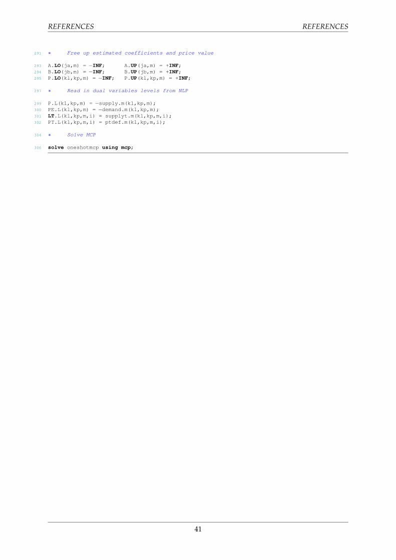
291 ∗ Free up estimated coefficients and price value

293 A.LO(ja,m) = −INF; A.UP(ja,m) = +INF;294 B.LO(jb,m) = −INF; B.UP(jb,m) = +INF;295 P.LO(kl,kp,m) = −INF; P.UP(kl,kp,m) = +INF;

297 ∗ Read in dual variables levels from NLP

299 P.L(kl,kp,m) = −supply.m(kl,kp,m);300 PE.L(kl,kp,m) = −demand.m(kl,kp,m);301 LT.L(kl,kp,m,i) = supplyt.m(kl,kp,m,i);302 PT.L(kl,kp,m,i) = ptdef.m(kl,kp,m,i);

304 ∗ Solve MCP

306 solve oneshotmcp using mcp;

41