Embed Size (px)
Citation preview
SOLVING LINEAR SYSTEMS OF EQUATIONS OVER
CYCLOTOMIC FIELDS
Liang Chen
BSc . Simon Fraser University, 2005
A THESIS SUBMITTED IN PARTIAL FULFILLMENT
O F T H E REQUIREMENTS FOR THE DEGREE O F
MASTER OF SCIENCE
in the School
of
Computing Science
@ Liang Chen 2007
SIMON FRASER UNIVERSITY
2007
All rights reserved. This work may not be
reproduced in whole or in part, by photocopy
or other means, without the permission of the author.
APPROVAL
Name:
Degree:
T i t l e of thesis:
Liang Chen
Master of Science
Solving Linear Systems of Equations over Cyclotomic Fields
Examining C o m m i t tee:
Chair
Date Approved:
Dr. Michael Monagan, Senior Supervisor
Associate Professor, Mathematics
Simon Fraser University
Dr. Petra Berenbrink, Supervisor
Assistant Professor, Computing Science
Simon Fraser University
Dr. Nils Bruin, SFU Examiner
Assistant Professor, Mathematics
Simon Fraser University

S I M O N F R A S E R U N I V E R S I T Y L I B R A R Y
Declaration of Partial Co~yright Licence The author, whose copyright is declared on the title page of this work, has granted to Simon Fraser University the right to lend this thesis, project or extended essay to users of the Simon Fraser University Library, and to make partial or single copies only for such users or in response to a request from the library of any other university, or other educational institution, on its own behalf or for one of its users.
The author has further granted permission to Simon Fraser University to keep or make a digital copy for use in its circulating collection (currently available to the public at the "Institutional Repository" link of the SFU Library website <www.lib.sfu.ca> at: <http://ir.lib.sfu.ca/handle/1892/112>) and, without changing the content, to translate the thesis/project or extended essays, if technically possible, to any medium or format for the purpose of preservation of the digital work.
The author has further agreed that permission for multiple copying of this work for scholarly purposes may be granted by either the author or the Dean of Graduate Studies.
It is understood that copying or publication of this work for financial gain shall not be allowed without the author's written permission.
Permission for public performance, or limited permission for private scholarly use, of any multimedia materials forming part of this work, may have been granted by the author. This information may be found on the separately catalogued multimedia material and in the signed Partial Copyright Licence.
While licensing SFU to permit the above uses, the author retains copyright in the thesis, project or extended essays, including the right to change the work for subsequent purposes, including editing and publishing the work in whole or in part, and licensing other parties, as the author may desire.
The original Partial Copyright Licence attesting to these terms, and signed by this author, may be found in the original bound copy of this work, retained in the Simon Fraser University Archive.
Simon Fraser University Library Burnaby, BC, Canada
Abstract
Let A E Q[zInxn be a matrix of polynomials and b E Q[zIn be a vector of polynomials.
Let m(z ) = Qk[z] be the kth cyclotomic polynomial. Wa want t o find thc solution vcctor
x E Q[zIn such that the equation Ax - b mod m(z ) holds. One may obtain x using Gaussian
elimination, howevcr, it is inefficierit bec:ausc of the large ratioiial rilirribcrs that appcar in thc
c:ocfficicrits of the polynomials in the matrix during thc elimination. In this thesis, wc prcsmt
two modular algorithms namely, Chinese remaindering and linear pad ic lifting. We have
implemented both algorithms in Maple and have determined the time complexity of both
algorithms. We preserit tirning cornparison tables on two sets of data, firstly, syster~is with
random generated coefficients and secondly real systems given to us by Vahid Dabbaghian
which arise from computational group theory. The results show that both of our algorithms
are much faster than Gaussian elimination.
Keywords: modular algorithm; cyclotomic fiald; Chinesa ramaindaring; pad ic lifting;
rational reconstruction

To my parents.
"Behind every argument is someone's ignorance."
- LOUIS D. BRANDEIS (1856 - 1941)
Acknowledgments
I would like to thank my parents who have always supported me in my studies, and especially
their support in the last 6 years of my studies in Canada. I cannot think of any other ways
to show my appreciation to them except trying my best in my studies.
I would also like to thank Dr. Michael Monagan, my senior supervisor, who brought me
into this research area. I met Dr. Monagan in September 2004 in the cryptography course
he was teaching. I was interested in this course because Dr. Xiaoyun Wang demonstrated
collision attacks against MD5, SHA-0 and some other related hash functions in August
2004 which was considered a big achievement in cryptography. By coincidence, Michael
was offering a course in cryptography in September 2004. Therefore, I joined his class and
explored the world of cryptography. In the following semester, I took the computer algebra
course with Michael as one of his graduate students, and then started to do research in
computer algebra with him. Michael made a grcat effort helping me work through my
research. I appreciate his patience and guidance.
My co-supervisor, Dr. Petra Berenbrink, is from the School of Computing Science who
does research in probabilistic methods, randomized algorithms, and parallel computing. She
has a very strong background in theory and I appreciate her guidance.
At last, I would like to thank my friends Simon, Al, Greg, and everyone in the CECM
lab. We had a great time together, and I really enjoyed being with you guys!
Contents
Approval ii
. . . Abstract 111
Dedication iv
Quotation v
Acknowledgments vi
Contents vii
List of Tables ix
List of Figures x
1 Introduction 1
1.1 Cyclotomic Fields and Cyclotomic Polynomials . . . . . . . . . . . . . . . . . 2
1.2 Polynomial Interpolation . . . . . . . . . . . . . . . . . . . . . . . . . . . . . . 3
1.3 Chinese Remaindering . . . . . . . . . . . . . . . . . . . . . . . . . . . . . . . 4
1.4 Rational Number Reconstruction . . . . . . . . . . . . . . . . . . . . . . . . . 7
1.4.1 Maximal Quotient Rational Reconstruction . . . . . . . . . . . . . . . 7
1.4.2 Runtime Complexity of Rational Number Reconstruction . . . . . . . 9
1.5 A padic Lifting Algorithm to Solve Ax = b over Q . . . . . . . . . . . . . . . 10
1.5.1 p-adic Representation of Integers . . . . . . . . . . . . . . . . . . . . . 10
1.6 Other Definitions, Results and Notations Used . . . . . . . . . . . . . . . . . 12
1.6.1 Definitions and Notations . . . . . . . . . . . . . . . . . . . . . . . . . 12
2 Algorithms 13
. . . . . . . . . . . . . . . . . . . . . . . . . . 2.1 Gaussian Elimination Approach 13
. . . . . . . . . . . . . . . . . . . . . . . . . . . . . . . . . 2.1.1 Description 13
. . . . . . . . . . . . . . . . . . . . . . . . . . . . . . 2.1.2 Runtime Analysis 14
. . . . . . . . . . . . . . . . . . . . . . . 2.1.3 Reduction to Solving over Q 14
. . . . . . . . . . . . . . . . . . . . . . . . . 2.2 Chinese Remaindering Approach 15
. . . . . . . . . . . . . . . . . . . . . . . . . . . . . . 2.2.1 The Subroutines 15
. . . . . . . . . . . . . . . . . . . . . . . . . . . . . . . 2.2.2 The Algorithm 17
. . . . . . . . . . . . . . . . . . . . . . . . 2.2.3 Correctness of Algorithm 1 19
. . . . . . . . . . . . . . . . . . . . . 2.2.4 Runtime Analysis of Algorithm 1 20
. . . . . . . . . . . . 2.2.5 Run Out of Primes Problem on 32 bit Machines 26
. . . . . . . . . . . . . . . . . . . . . . . . . . 2.3 Linear padic Lifting Approach 26
. . . . . . . . . . . . . . . . . . . . . . . . . . . . . . . . . 2.3.1 Description 26
. . . . . . . . . . . . . . . . . . . . . . . . . . . . . . 2.3.2 The Subroutines 27
. . . . . . . . . . . . . . . . . . . . . . . . . . . . . . . 2.3.3 The Algorithm 29
. . . . . . . . . . . . . . . . . . . . . 2.3.4 Runtime Analysis of Algorithm 2 29
. . . . . . . . . . . . . . . . . . . . . . . . 2.3.5 Computing the Error Term 34
. . . . . . . . . . . . 2.3.6 Attempt at a Quadratic padic Lifting Approach 37
. . . . . . . . . 2.4 An Upper Bound of the Coefficients in the Solution Vector x 37
. . . . . . . . . . . . 2.4.1 The Hadamard Maximum Determinant Problem 37
2.4.2 A Hadamard-Type Bound on the Coefficients of a Determinant of a
Matrix of Polynomials . . . . . . . . . . . . . . . . . . . . . . . . . . . 37
. . . . . . . . . . . . . . . . . . . . . . . . . 2.5 Runtime Complexity Comparison 39
. . . . . . . . . . . . . . . . . . . . . . . . . . . 2.6 Implementation and Timings 40
. . . . . . . . . . . . . 2.6.1 Timing the Random Systems and Real Systems 40
3 Conclusion 45
Bibliography 46
... Vl l l
List of Tables
Examples of the first ten cyclotomic polynomials. are some of the corre-
sponding complex root(s) . . . . . . . . . . . . . . . . . . . . . . . . . . . . . 3
Runtime (in CPU seconds) of Random dense input with various dimensions
and coefficients. "-" denotes the running time is over 5,000 seconds. . . . . . 43
Runtime (in CPU seconds) on some of the systems given by Vahid Dabbaghian. 44
Runtime (in CPU seconds) on some of the huge systems given by Vahid Dab-
baghian. "-" denotes the running time is over 50,000 seconds. "*" denotes
. . . . . . . . . . . . . . . . . . . . . . . . . . . . . . . . . run out of memory. 44
List of Figures
2.1 Process flow of the Chinese remaindering approach . . . . . . . . . . . . . . . 18
2.2 Process flow of the linear padic lifting approach . . . . . . . . . . . . . . . . 28
Chapter 1
Introduction
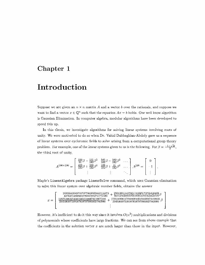
Suppose we are given an n x n matrix A and a vector b over the rationals, and suppose we
want t o find a vector x E Qn such that the equation Ax = b holds. One well know algorithm
is Gaussian Elimination. In computer algebra, modular algorithms have been developed to
speed this up.
In this thesis, we investigate algorithms for solving linear systems involving roots of
unity. We were motivated to do so when Dr. Vahid Dabbaghian-Abdoly gave us a sequence
of linear systems over cyclotomic fields to solve arising from a computational group theory
problem. For example, one of the linear systems given to us is the following. For /3 = q, the third root of unity,
Maple's LinearAlgebra package Linearsolve command, which uses Gaussian elimination
to solve this linear system over algebraic number fields, obtains the answer
However, it's inefficient to do it this way since it involves 0(n3) multiplications and divisions
of polynomials whose coefficients have large fractions. We can see from above example that
the coefficients in the solution vector x are much larger than those in the input. However,
CHAPTER 1. INTRODUCTION 2
they are a lot smaller than the maximum possible coefficient if the coefficients in input
matrix A and vector b were of the same size as in the example, i.e., < lo3, but generated
randomly. We should design the algorithms in such a way that the work they do is less
if the output is small. For such random input, we obtain the maximum coefficient in the
solution vector x to be about 9452 bits long by experiment, and it takes a "long time" (see
Tables 2.1, 2.2, 2.3) for Gaussian elimination to obtain the solution of such a system. In
Chapter 2, we develop two efficient rnodular algorithms namely Chinese remairlderirig arid
linear padic lifting. Both of the algorithms need to use rational number reconstruction to
recover the rational coefficients in the solution vector as in the above example.
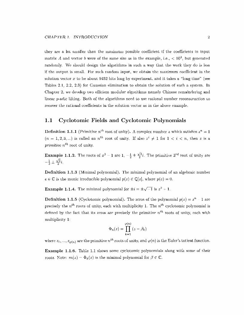
1.1 Cyclotomic Fields and Cyclotomic Polynomials
Definition 1.1.1 (Primitive nth root of unity). A complex number z which satisfies zn = 1
(n = 1 ,2 ,3 , ...) is called an nth root of unity. If also zi # 1 for 1 < i < n , then z is a
primitive nth root of unity.
Example 1.1.2. The roots of x3 - 1 are 1, -1 f $1. The primitive 3Td root of unity are -1 f g,,
2
Definition 1.1.3 (Minimal polynomial). The minimal polynomial of an algebraic number
e E @ is the monic irreducible polynomial p(z) E Q[z], where p(e) = 0.
Example 1.1.4. The minimal polynomial for f i = f a is z2 + 1.
Definition 1.1.5 (Cyclotomic polynomial). The zeros of the polynomial p(z) = zn - 1 are
precisely the nth roots of unity, each with multiplicity 1. The nth cyclotomic polynomial is
defined by the fact that its zeros are precisely the primitive nth roots of unity, each with
multiplicity 1:
where zl , ..., zV(,) are the primitive nth roots of unity, and p(n) is the Euler7s totient function.
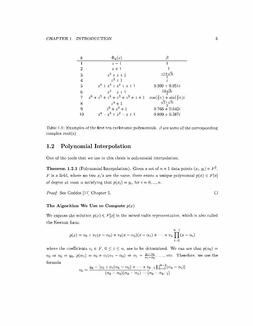
Example 1.1.6. Table 1.1 shows some cyclotomic polynomials along with some of their
roots. Note: m(z) = Qk(z) is the minimal polynomial for P E @.
CHAPTER 1. INTRODUCTION
Table 1.1: Examples of the first ten cyclotomic polynomials. f i are some of the corresponding complex root(s)
1.2 Polynomial Interpolation
One of the tools that we use in this thesis is polynomial interpolation.
Theorem 1.2.1 (Polynomial Interpolation). Given a set of n + 1 data points (xi, yi) E F ~ ,
F is a field, where no two xi's are the same, there exists a unique polynomial p(x) E F[x]
of degree at most n satisfying that p(xi) = yi, for i = 0 , ..., n.
Proof. See Geddes [ll] Chapter 5 . 0
The Algorithm We Use to Compute p(x)
We express the solution p(x) E F[x] in the mixed radix representation, which is also called
the Newton form:
n-1
p(x) = v o + v l ( x - no) +v2(x - ao)(x - 01) + . . + v , n ( x - a i ) i=o
where thc coefficients v, E F, 0 < i < n , are to be determined. We can see that p(cuo) =
vO + vO = yo, p(nl) = + vl(nl - no) + v1 = E, . . ., etc. Therefore, we use the

CHAPTER 1. INTRODUCTION 4
to calculate vk for 0 < /c < n to obtain p(z). This interpolation method takes 0 ( n 2 )
arithmetic operations in F to obtain p(x) where n is the number of pairs of evaluation
points.
Example 1.2.2. Given three points (-5,3), (0,8), (10, -2), wc want to find thc quadratic
polynomial p(x) E Q[x] such that p(-5) = 3, p(0) = 8, and p(10) = -2.
Using the Newton's interpolation we have the polynomial p(x) in the form:
P(X) = vo + v 1 ( x + 5 ) +v2(x+5) (x - O),
and we would like to solve for vo, vl, and v2. We know p(-5) = vo = 3, therefore vo = 3;
p(0) = 3 + vl (0 + 5) = 8, therefore vl = 1; p(10) = 3 + l(10 + 5) + v2(10 + 5)(10 - 0) = -2,
therefore v2 = - &. Hence we obtain
Remark: Maple uses Newton's polynomial interpolation which takes O(n2) operations in
F for n pairs of evaluation points of constant lengths. One may use Lagrange interpolation
instead which also takes O(n2) operations in F to compute.
1.3 Chinese Remaindering
We realize that computing with single-precision integers is considerably more efficient than
computing with multiprecision integers. Therefore, we may transform a computation involv-
ing large integers into a computation with integers that can be fit into one computer word,
and then recover the multiprecision integers in the solution. In this section, we discuss the
Chinese remainder theorem and Chinese remainder algorithm which recovers multiprecision
integers from a sequence of single-precision integers.
Theorem 1.3.1 (Chinese Remainder Theorem). Let mo, ml , .. . , mn E Z be integers which
are pairwise relatively prime and let ui E Z, i = 0,1, ..., n be n + 1 specified residues. For
any fixed integer a E Z there exists a unique integer u E Z which satisfies the following
conditions: n
u = u i (mod mi), 0 5 i s n . , a n d a s u< a + m , wherem= n m i . (1.1) i=O
Proof. See Geddes [ll] Chapter 5. 0
CHAPTER 1. INTRODUCTION 5
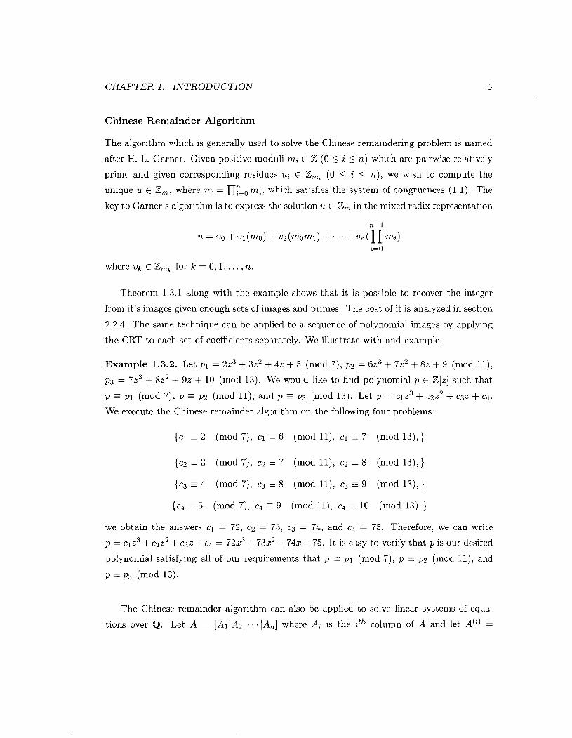
Chinese Remainder Algorithm
The algorithm which is generally used to solve the Chinese remaindering problem is named
after H. L. Garner. Given positive moduli mi E Z ( 0 5 i < n) which are pairwise relatively
prime and given corresponding residues ui E Zmt ( 0 < i < n) , we wish to compute the
unique u E Z,, where m = nLo mi, which satisfies the system of congruences (1 .1) . The
key to Garner's algorithm is to express the solution u E Z , in the mixed radix representation
n-1
u = uo + u l ( m o ) + v ~ ( m o m 1 ) + . . + u n ( n mi)
i=O
where vk E Z,, for k = 0 , 1 , . . . , n .
Theorem 1.3.1 along with the example shows that it is possible to recover the integer
from it's images given enough sets of images and primes. The cost of it is analyzed in section
2.2.4. The same technique can be applied to a sequence of polynomial images by applying
the CRT to each set of coefficients separately. We illustrate with and example.
Example 1.3.2. Let pi = 22% 3z2 + 4z + 5 (mod 7 ) , p2 = 6z3 + 7 z 2 + 8z + 9 (mod l l ) ,
p3 = 7z3 + 8z2 + 9z + 10 (mod 13). We would like to find polynomial p E Z [ z ] such that
p - pi (mod 7 ) , p -- p2 (mod l l ) , and p - p3 (mod 13). Let p = c1z3 + c2z2 + c3z + c4.
We execute the Chinese remainder algorithm on the following four problems:
{c l - 2 (mod 7 ) , cl -- 6 (mod l l ) , cl - 7 (mod 13) ,
{cz r 3 (mod 7 ) , c2 -- 7 (mod l l ) , c2 = 8 (mod 13) ,
{cg -- 4 (mod 7 ) , c3 = 8 (mod l l ) , cg -- 9 (mod 13) ,
{ c ~ -- 5 (mod 7 ) , c4 - 9 (mod l l ) , c4 - 10 (mod 13) , }
we obtain the answers cl = 72, c2 = 73, c3 = 74, and c4 = 75. Therefore, we can write
p = clz% c2z2 + c3.z + c4 = 72x3 + 732' + 742 + 75. It is easy to verify that p is our desired
polynomial satisfying all of our requirements that p E pl (mod 7 ) , p - p2 (mod l l ) , and
p =p3 (mod 13).
The Chinese remainder algorithm can also be applied to solve linear systems of equa-
tions over Q. Let A = [ A l [ A 2 1 . . . / A n ] where Ai is the ith column of A and let A(') =
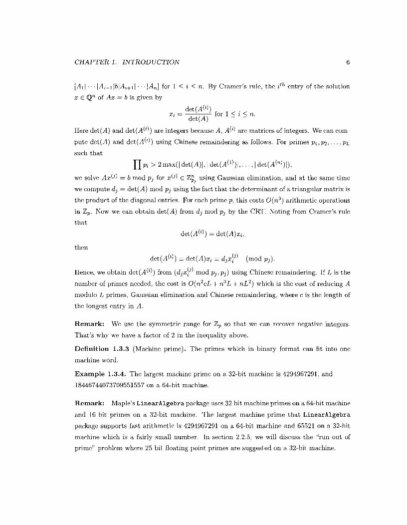
CHAPTER 1. INTRODUCTION 6
[All . . . IAi-llblAi+ll . . . IA,] for 1 < i 5 n. By Cramer's rule, the ith entry of the solution
x E Qn of Ax = b is given by
xi = det ( A ( ~ ) )
for 15 i 5 n. det (A)
Here det(A) and d e t ( ~ ( ~ ) ) are integers because A, A ( ~ ) are matrices of integers. We can corn-
pute det(A) and d e t ( ~ ( ~ ) ) using Chinese remaindering as follows. For primes pl, p2,. . . , p~
such that n Pi > 2 max(1 det(A) 1 , I det (A(')) 1 , . . . , I det (A(")) I),
we solve AX(^) = b mod p j for x(j) E ZT2 using Gaussian elimination, and at the same time
we compute dj = det(A) mod p j using the fact that the determinant of a triangular matrix is
the product of the diagonal entries. For each prime p, this costs O(n3) arithmetic operations
in Zp. Now we can obtain det(A) from d j mod pJ by the CRT. Noting from Cramer's rule
that
d e t ( ~ ( ~ ) ) = det(A)xi,
then
d e t ( ~ ( ' ) ) = det(A)xi = djx?) (mod pj).
Hence, we obtain det(A(')) from ( d j ~ / ~ ) mod pj ,pj) using Chinese remaindering. If L is the
number of primes needed, the cost is 0(n2cL + n3L + nL2) which is the cost of reducing A
modulo L primes, Gaussian elimination and Chinese remaindering, where c is the length of
the longest entry in A.
Remark: We use the symmetric range for Z p SO that we can recover negative integers.
That's why we have a factor of 2 in the inequality above.
Definition 1.3.3 (Machine prime). The primes which in binary format can fit into one
machine word.
Example 1.3.4. The largest machine prime on a 32-bit machine is 4294967291, and
18446744073709551557 on a 64-bit machine.
Remark: Maple's LinearAlgebra package uses 32 bit machine primes on a 64-bit machine
and 16 bit primes on a 32-bit machine. The largest machine prime that LinearAlgebra
package supports fast arithmetic is 4294967291 on a 64-bit machine and 65521 on a 32-bit
machine which is a fairly small number. In section 2.2.5, we will discuss the "run out of
prime" problem where 25 bit floating point primes are suggested on a 32-bit machine.
CHAPTER 1. INTRODUCTION
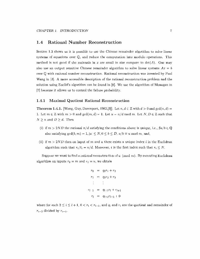
1.4 Rational Number Reconstruction
Section 1.3 shows us it is possible to use the Chinese remainder algorithm to solve linear
systems of equations over Q, and reduce the computation into modulo operations. This
method is not good if the rationals in x are small in size compare to det(A). One may
also use an output sensitive Chinese remainder algorithm to solve linear systems Ax = b
over Q with rational number reconstruction. Rational reconstruction was invented by Paul
Wang in [3]. A more accessible description of the rational reconstruction problem and the
solution using Euclid's algorithm can be found in [8]. We use the algorithm of Monagan in
[7] because it allows us to control the failure probability.
1.4.1 Maximal Quotient Rational Reconstruction
Theorem 1.4.1. [Wang, Guy, Davenport, 1982,[3]]. Let n, d E Z with d > 0 and gcd(n, d) =
1. Let m E Z with m > 0 and gcd(m, d) = 1. Let u = n l d mod m. Let N, D E Z such that
N > n and D > d. Then
(i) if m > 2ND the rational n l d satisfying the conditions above is unique, i.e., $a/b E Q
also satisfying gcd(b, m) = 1, l a < N, 0 5 b 5 D , a lb - u mod m, and,
(ii) if m > 2 N D then on input of m and u there exists a unique index i in the Euclidean
algorithm such that r i / t i = nld . Moreover, i is the first index such that ri < N.
Suppose wt: want to firid a rational rec:oristruc:tion of u (mod m). By executing Euclidean
algorithm on inputs ro = m and rl = u, we obtain
where for each 2 5 i < 1 + 1, 0 < ri < ri-1, and qi and ri are the quotient and remainder of
ri-2 divided by ri-1.

CHAPTER 1. INTRODUCTION
Also, for any 2 5 i 5 1 + 1, the equation
ri = tire + sir1
holds for some integers ti , si, and the values of ti and si can be obtained from the the
extended Euclidean algorithm. Then for si and m are relatively prime, we obtain:
u = r i / s i (modm).
Example 1.4.2. Suppose n / d = 13/10 and suppose we have computed n / d mod 997 and
n / d mod 1009. Then we apply the Chinese remainder algorithm we obtain u = 905377
wliidi satisfies u = n l d mod m where m = 997 x 1009 = 1005973. If we apply Euclidean
algorithm on u and m, we obtain
1005973 = 1 x 905377 + 100596
905377 = 9 x 100596 + 13
100596 = 7738 x 13 + 2
13 = 6 x 2 + 1
2 = 2 x 1 + 0 .
We obtain these equations and rationals u' with u' = u (mod m):
The maximal quotient rational reconstruction algorithm outputs the rational r i / s i for
which qi+l is the maximal quotient, i.e., 13/10 in our example. The idea of this algorithm
is to output the smallest rational r i / s i . Lemma 1.4.3 shows how the size of the quotient
qi+l relates to the size of the rational r i / t i and the modulus m over iterations of Euclidean
algorithm.
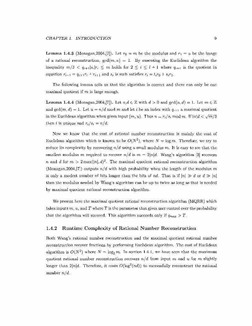
CHAPTER 1. INTRODUCTION 9
Lemma 1.4.3 (Monagan,2004,[7]). Let ro = m be the modulus and rl = u be the image
of a rational reconstruction, gcd(m,u) = 1. By executing the Euclidean algorithm the
inequality m/3 < qi+lls,lri 5 m holds for 2 5 i 5 1 + 1 where qi+l is the quotient in
equation ri-1 = qi+lri + ri+l and si is such satisfies ri = tire + s i r l .
The following lemma tells us that the algorithm is correct and there can only be one
maximal quotient if m is large enough.
Lemma 1.4.4 (Monagan,2004,[7]). Let n,d E Z with d > 0 and gcd(n, d) = 1. Let m E Z
and gcd(m, d) = 1. Let u = n/d mod m and let i be an index with qi+l a maximal quotient
in the Euclidean algorithm when given input (m , u) . Thus u - r,/si mod m. If In(d < 6 1 3
then i is unique and ri/si = n ld .
Now we know that the cost of rational number reconstruction is mainly the cost of
Euclidean algorithm which is known to be O(N2) , where N = log m. Therefore, we try to
reduce its complexity by recovering n/d using a small modulus m. It is easy to see that the
smallest modulus m required to recover n/d is m = 21nld. Wang's algorithm [3] recovers
n and d for m > 2max(lnl, d)2. The maximal quotient rational reconstruction algorithm
(Monagan,2004,[7]) outputs n/d with high probability when the length of the modulus m
is only a modest number of bits longer than the bits of nd. That is if In1 >> d or d >> In1
then the modulus needed by Wang's algorithm can be up to twice as long as that is needed
by maximal quotient rational reconstruction algorithm.
We present here the maximal quotient rational reconstruction algorithm (MQRR) which
takes inputs m , u , and T where T is the parameter that gives user control over the probability
that the algorithm will succeed. This algorithm succeeds only if q,,, > T.
1.4.2 Runtime Complexity of Rational Number Reconstruction
Both Wang's rational number reconstruction and the maximal quotient rational number
reconstruction recover fractions by performing Euclidean algorithm. The cost of Euclidean
algorithm is o ( N ~ ) where N = log2 m. In section 1.4.1, we have seen that the maximum
quotient rational number reconstruction recovers n/d from input m and u for m slightly
longer than 21nld. Therefore, it costs 0(log2(nd)) to successfully reconstruct the rational
number n/d.
CHAPTER 1. INTRODUCTION 10
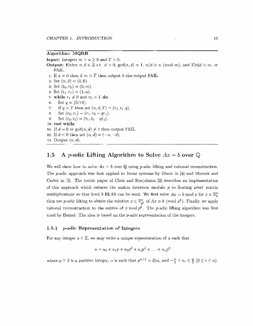
Algorithm: MQRR Input: Integers m > u 2 0 and T > 0. Output: Either n , d E Z s.t. d > 0, gcd(n,d) = 1, n l d - u (mod m) , and Tlnld < m, or
FAIL. 1: If u = 0 then if m > T then output 0 else output FAIL. 2: Set (n , d) = (0,O). 3: Set (to, TO) = (0, m) . 4: Set ( t l , r l ) = (1 ,u) . 5: while rl # 0 and ro > T do 6: Set q = LOlrl]. 7: I f q > T t h e n s e t ( n , d , T ) = ( r l , t l , q ) . 8: Set (TO, 7-1) = ( r l , ro - qrl). 9: Set (to, t l ) = ( t l , to - qtl).
lo: end while 11: If d = 0 or gcd(n, d) # 1 then output FAIL. 12: If d < 0 then set (n, d) = (-n, -d). 13: Output (72, d).
1.5 A p-adic Lifting Algorithm to Solve Ax = b over Q
We will show how to solve A x = b over Q using padic lifting and rational reconstruction.
The padic approach was first applied to linear systems by Dixon in [4] and Moenck and
Carter in [5] . The recent paper of Chen and Storjohann [2] describes an implementation
of this approach which reduces the matrix inversion modulo p to floating point matrix
multiplications so that level 3 BLAS can be used. We first solve A x = b mod p for x E Z i
then use padic lifting to obtain the solution x E Zi, of A x = b (mod p k ) . Finally, we apply
rational reconstruction to the entries of x mod pk. The pad ic lifting algorithm was first
tried by Hensel. The idea is based on the padic representation of the integers.
1.5.1 padic Representation of Integers
For any integer u E Z, we may write a unique representation of u such that
where p > 2 is a positive integer, 72 is such that pnfl > 21~1, and - 5 5 ui < 5 (0 < i < n).

CHAPTER 1. INTRODUCTION
padic Representation of Integer Vectors
For an integer vector V E Zn, we may also write V in the form
For example, Let V = [9, -80,94IT, and p = 13. We may obtain = 1-4, -2,3IT, by
the operation V (mod p) in symmetric range, and & = E& (mod p) = [l, -6, -6IT, and P
V2 = (mod p) = [O, 0, 1IT. Therefore, we obtain the unique padic representation P
V = Vo + Vlp + v~~~ = [-4, -2, 3IT + 13[1, -6, -6IT + 132[0,0, 1IT.
Solving Linear Systems of Equations Ax = b over Q
We now apply padic lifting algorithm to solve linear systems of equations over Q. For
I -25 -44 86
example, let A = 51 24 20 1 , b = [ I , 2, 3IT, and p = 13. Wc would like to find
1 7 6 65 - 6 1 1 vector x such that Ax = b.
First of all, let us show a general solution to this system. Let x ( ~ ) = xo + xlp + . . . + xk-lpk-l be the solution of Ax - b mod pk, i.e., x ( ~ ) is the kth order approximation of
x. Therefore, we can find the first order approximation x(l) = s o by solving the equation
Axo - b mod p. Assuming we know x ( ~ ) for k > 1, the (k + l)th order approximation, i.e.,
x ( ~ + ' ) , can be determined by the kth order approximation x ( ~ ) and the equation AX(^+') =
b mod pk+l from
AX("') = A ( x ( ~ ) + xkpk) c) b mod pk+l.
Since A, b, and x ( ~ ) are known, we can then obtain xk from the above equation hence
x("l). In our example, the first order approximation x(l) = xo = [4,5, 6IT is obtained
by solving the equation Axo = b (mod p) in the symmetric range. Then we obtain xl =
b - A x ( l ) (mod p), and so on. Noting that, the solution [-5,3, -11 from the equation Axl = - P
vector is lifted to in the kth iteration, however, we may never balance the equation
A(xo + xlp + . . . + xlpl) = b for any 1 E Z if the true solution vector x has fractions in its
entries. Rational number reconstruction is used to solve this problem. We apply rational
number reconstructions to x ( ~ ) mod pk for k = 1 ,2 ,3 , . . . to obtain y(k) E Qn. We stop when
A ~ ( ~ ) = b. In our example, we try to compute images of x and do rational reconstruction till

CHAPTER 1. INTRODUCTION 12
x ( ~ ) = x0 + x ~ p + x2p2 + x3p3 + x4p4 + x5p5 + x6p6 which we successfully recovered the fraction 995 T entries using maximal quotient rational reconstruction and obtain x = [z, - a , - .
1.6 Other Definitions, Results and Notations Used
1.6.1 Definitions and Notations
We now define some notations and state some techniques that will be used in the imple-
mentation and analysis of our modular algorithms.
Let m ( z ) be a polynomial in z with integer cocficicnts. Wc dcriotc the rnaxirriurn of the
absolute value of coefficients in m ( z ) by I lml loo .
Definition 1.6.1. We define in our paper t,hat the lengt,h (or size) of a rational number
n l d is the length of the absolute value of the product of n and dl i.e., log Indl.
Let M be a matrix or vector of polynomials with rational coefficients. Let n l d be the
rational coefficient such that is the largest in length. We denote the value lndl by IIMlloo.
Single-Point Evaluation and Interpolation
Consider the problem of computing c ( z ) = a ( z ) x b( z ) E Z [ z ] , where a ( z ) = z3 + 5z2 + 32 + 6 ,
b ( z ) = 2z2 +3z+ 1. Let < E Z be a positive integer which bounds 21 Ic(z)ll,. We substitute < into a ( z ) and b ( z ) and compute their product. We choose < = 1000 for simplicity. We have,
a(<) = 1005003006, b(<) = 2003001, hence c(<) = a(<) x b(<) = 1005003006 x 2003001 =
2013022026021006. Now, we do single-point interpolation at z = 1000 and obtain c ( z ) =
2z5 + 13z4 + 22z3 + 26z2 + 212 + 6 from c(<). Is c ( z ) precisely the product of a ( z ) and b(z)?
It must be if < > 211clloo.
Remark: One should choose < = Bm where B is the base of the integer system so that
evaluation and single-point interpolation are linear time. This method works the same for
polynomials with negative coefficients if we use symmetric range in the interpolation step.
Chapter 2
Algorithms
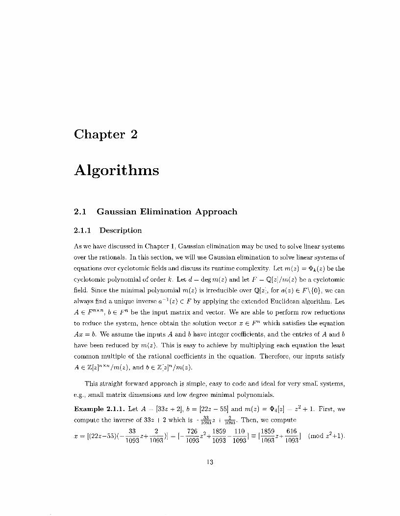
2.1 Gaussian Elimination Approach
2.1.1 Description
As we have discussed in Chapter 1, Gaussian elimination may be used to solve linear systems
over the rationals. In this section, we will use Gaussian elimination to solve linear systems of
equations over cyclotomic fields a.nd discuss its runtime complexity. Let m(z) = Qk(z) be the
cyclotomic polynomial of order k. Let d = degm(z) and let F = Q[z]/m(z) be a cyclotomic
field. Since the minimal polynomial m(z) is irreducible over Q[z], for a(z) E F\{O}, we ca.n
always find a unique inverse aP1(z) E F by applying the extended Euclidean algorithm. Let
A E Fnxn, b E Fn be the input matrix and vector. We are able to perform row reductions
to reduce the system, hence obtain the solution vector x E Fn which satisfies the equation
A x = b. We assume the inputs A and b have integer coefficients, and the entries of A and b
have been reduced by m(z) . This is easy to achieve by multiplying each equation the least
common multiple of the rational coefficients in the equation. Therefore, our inputs satisfy
A E Z[zInxn/m(z), and b E Z[zIn/m(z).
This straight forward approach is simple, easy to code and ideal for very small systems,
e g . , small matrix dimensions and low degree minimal polynomials.
Example 2.1.1. Let A = [332 + 21, b = [222 - 551 and m(z) = Q4[z] = z2 + 1. First, we
compute the inverse of 332 + 2 which is -&z + A. Then, we compute
33 2 726 , 1859 110 1859 616 z+-] (mod z2+l) . x = [(22~-55)(--2+-)1 = [kE2 +1093-ml -
1093 1093 1093

CHAPTER 2. ALGORITHMS 14
In calculating x, we run the Euclidean algorithm in the ring Q[z], then do polynomial
mnltiplication, and finally a polynomial division by m(z). We can see in our example that the
maximum cocfficicnt lcngth in t,hc input matrix A and vector b is 2 decimal digits. However,
during our calculation, the maximal cocfficicnt lcngth in A-l increases to 6 decimal digits,
and the rnaxirnwri cocfficicnt lcngth in tlic solution vcctor increases t,o 7 decimal digits. For
large random inputs, i.e., n large, d large, we may get cocfficicnt,~ in solutiori vectors with
nd times the length of the maximal coefficicnt length in the inputs.
2.1.2 Runtime Analysis
Before we analyze the runtime, we define some notations for our problem. Let A E
Z[zInxn/m(z) and b E Z[zIn/m(z) be our input matrix and vector, and m(z) = a k ( z )
be the minimal polynomial. Let c = log max(IJAI I,, I Ibll,) dcnotc the maximum coefficient,
length in the input matrix and vector and let d = deg m(z). We assume that the maxi-
rrilirri length of the rational cocfficicnts in t,hc solut,ion vector x E Q[zIn/m(z) is L, that is
1% llxllm E O(L).
Since we know that Gaussian elimination over Q involves O(n3) multiplications over Q,
we expect O(n3) multiplications in the field F = Q[z]/m(z) and O(n) calls to the Euclidean
algorithm for inverses in F. Assuming classical algorithms for polynomial arithmetic, Gaus-
sian elimination over F costs O(n3d2) arithmetic operations over Q, but the size of the
rationals grows. Each polynomial multiplication takes 0(d212) operations where 1 is the
maximum coefficient length of the polynomials. We take 1 = $ which is the average length
of t,hc polynomial coefficients in the comput,ation, and obtain its runtime complexity to bc
O(n3d2L2) using classical, i.e., quadratic, algorithms for integers and polynomials.
2.1.3 Reduction to Solving over Q
The solution vector x E Fn of the linear system in section 2.1.1 is a vector of polynomials in
z of degree < d - 1 over Q where d = degm(z). Writing xi = ~ , d _ : nijzj for i = 1 ,2 , . . . , n
for unknown coefficients aij , if we multiply out Ax - b = 0 and divide by m(z) and equate
coefficients of 23 to zero, we obtain an nd by nd linear system over Q. This can be solved
using Gaussian elimination in O(n3d") arithmetic operations over Q. This reduction to Q
is not a good method. It increases the cost by a factor of d arithmetic operations over Q
when compared with the direct method in section 2.1.1.
C H A P T E R 2. ALGORITHMS
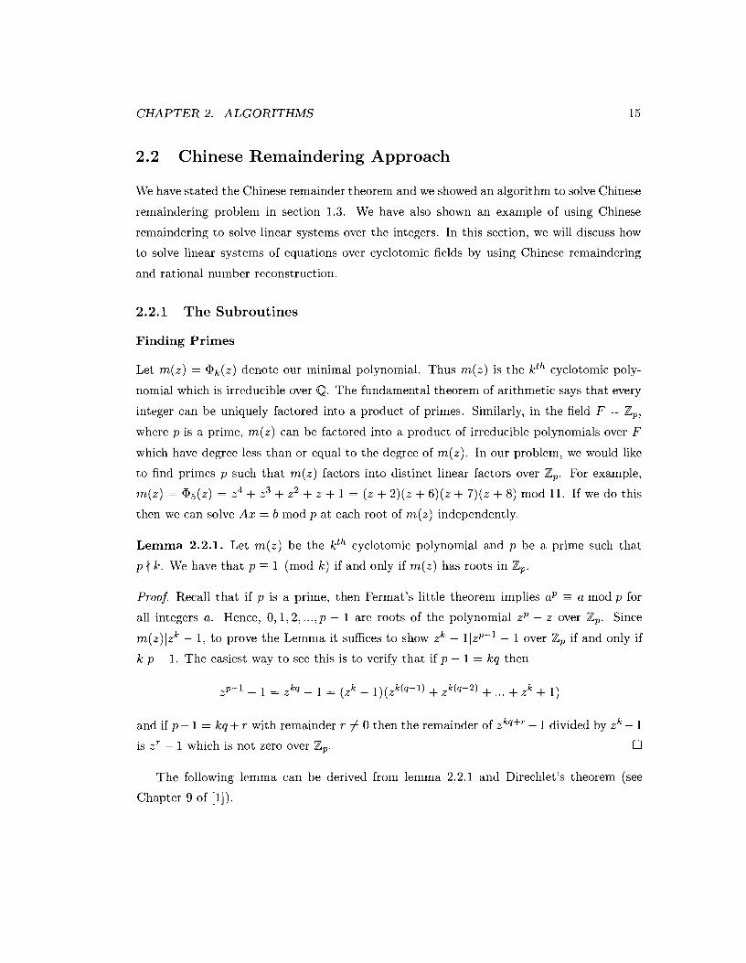
2.2 Chinese Remaindering Approach
We have stated the Chinese remainder theorem and we showed an algorithm to solve Chinese
remaindering problem in section 1.3. We have also shown an example of using Chinese
remaindering to solve linear systems over the integers. In this section, we will discuss how
to solve linear systems of equations over cyclotomic fields by using Chinese remaindering
and rational number reconstruction.
2.2.1 The Subroutines
Finding Primes
Let m(z) = a k ( z ) denote our minimal polynomial. Thus m(z) is the kth cyclotomic poly-
nomial which is irreducible over Q. The fundamental theorem of arithmetic says that every
integer can be uniquely factored into a product of primes. Similarly, in the field F = Zp,
where p is a prime, m(z) can be factored into a product of irreducible polynomials over F
which have degree less than or equal to the degree of m(z). In our problem, we would like
to find primes p such that m(z) factors into distinct linear factors over Zp. For example,
m(z) = a 5 ( z ) = z4 + z3 + z2 + z + 1 = (Z + 2)(z + 6)(z + 7)(z + 8) mod 11. If we do this
then we can solve Ax = b mod p at each root of m(z) independently.
Lemma 2.2.1. Let m(z) be the kth cyclotomic polynomial and p be a prime such that
p I j k. We have that p -- 1 (mod k) if and only if m(z) has roots in Z,.
Proof. Recall that if p is a prime, then Fermat's little theorem implies ap -- a mod p for
all integers a. Hence, O,1,2, ..., p - 1 are roots of the polynomial zp - z over Zp. Since
m(z)lzk - 1, to prove the Lemma it suffices to show zk - llzp-I - 1 over Zp if and only if
kip - 1. The easiest way to see this is to verify that if p - 1 = kg then
and if p - 1 = kg + r with remainder r # 0 then the remainder of zk4+' - 1 divided by zk - 1
is zr - 1 which is not zero over Zp. 0
The following lemma can be derived from lemma 2.2.1 and Direchlet's theorem (see
Chapter 9 of [I]).
C H A P T E R 2. ALGORITHMS 16
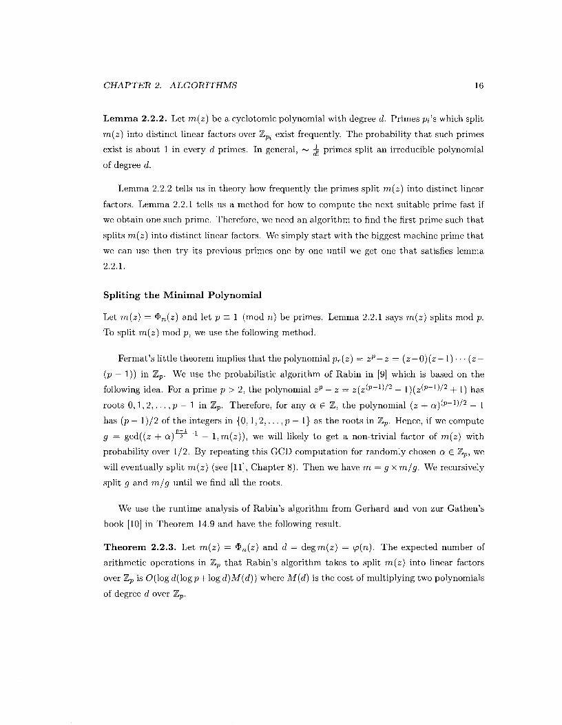
Lemma 2.2.2. Let m(z ) be a cyclotomic polynomial with degree d. Primes pi's which split
m(z) into distinct linear factors over Zpi exist frequently. The probability that such primes
exist is about 1 in every d primes. In general, primes split an irreducible polynomial
of degree d.
Lemma 2.2.2 tells us in theory how frequently the primes split m(z) into distinct linear
factors. Lemma 2.2.1 tells us a method for how to compute the next suitable prime fast if
we obtain one such prime. Therefore, we need an algorithm to find the first prime such that
splits m(z) into distinct linear factors. We simply start with the biggest machine prime that
we can use then try its previous primes one by one until we get one that satisfies lemma
2.2.1.
Spliting the Minimal Polynomial
Let m(z) = Qn(z) and let p - 1 (mod n) be primes. Lemma 2.2.1 says m(z) splits mod p.
To split m(z) mod p, we use the following method.
Fermat's little theorem implies that the polynomial p,(z) = zp- z = (z-O)(z- 1) . . . (z-
(p - 1)) in Zp. We use the probabilistic algorithm of Rabin in [9] which is based on the
following idea. For a prime p > 2, the polynomial zp - z = z ( z ( ~ - l ) / ~ - l ) ( z ( ~ - ' ) / ~ + 1) has
roots O,1,2, . . . , p - 1 in Zp. Therefore, for any a E Z, the polynomial (z + a)(p-l)12 - 1
has (p - 1)/2 of the integers in { O , 1 , 2 , . . . , p - 1) as the roots in Zp. Hence, if we compute "-1-1
g = gcd((z + a ) 2 - l , m ( z ) ) , we will likely to get a non-trivial factor of m(z) with
probability over 112. By repeating this GCD computation for randomly chosen a E Zp, we
will eventually split m(z) (see [ll], Chapter 8). Then we have m = g x mlg . We recursively
split g and m/g until we find all the roots.
We use the runtime analysis of Rabin's algorithm from Gerhard and von zur Gathen's
book [lo] in Theorem 14.9 and have the following result.
Theorem 2.2.3. Let m(z) = Qn(z) and d = deg m(z) = p(n) . The expected number of
arithmetic operations in Zp that Rabin's algorithm takes to split m(z) into linear factors
over Zp is O(1og d(logp+log d)M(d)) where M(d) is the cost of multiplying two polynomials
of degree d over Z,.
CHAPTER 2. ALGORITHMS 17
Note, the first contribution to the cost, logd logpM(d) , is the repeated squaring cost
and the second contribution, log2 d M ( d ) , is the GCD computation cost. If one uses clas-
sical quadratic algorithms for univariate polynomial multiplication and GCD, the expected
running time is O(log d2 log d) .
Rational Number Reconstruction
In Chapter 1 we have discussed how to recover a rational number with fractions from its
image. We apply this technique to recover the rational coefficients of a polynomial from its
image modulo m. For example, let pl = 15412z3 + 21025z2 + 77132 + 13504, m l = 23117 be
an image polynomial. We would like to find polynomial p E Q[z] such that p - pl (mod ml ) .
By executing maximal quotient rational reconstruction on each coefficient independently,
weget $ = 15412 (mod23117), = 21025 (mod23117), = 7713 (mod23117), and
& = 13504 (mod 23117) to be the coefficients of our original polynomial p = $x3 + $x2 + 22 1 3 x + m .
2.2.2 The Algorithm
By utilizing the above algorithms along with the polynomial evaluation and interpolation
algorithms that we have discussed in section 1.2, we can now present our first main algorithm.
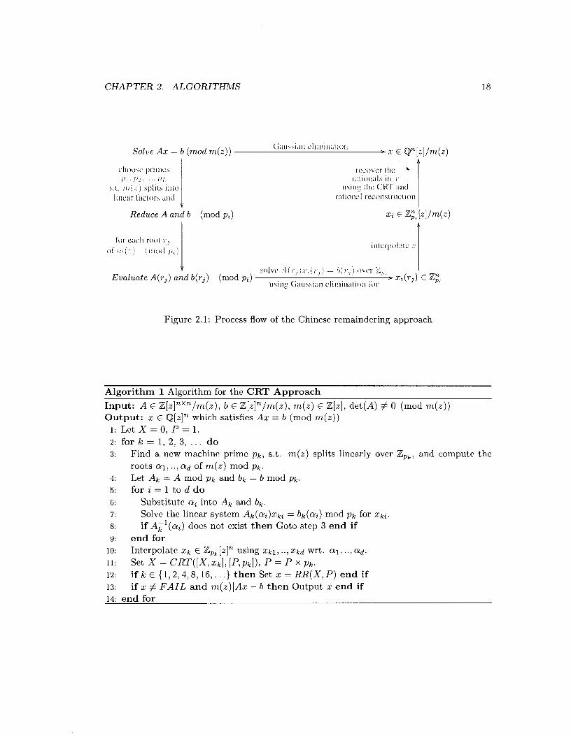
Figure 2.1 shows the main process flow of the Chinese remaindering approach. We divide
the process into 5 main phases. The first phase is t o choose primes such that our minimal
polynomial m(z) can be factored into distinct linear factors, and then reduce the coefficients
in the input A, b modulo those primes. The second phase is to compute all the roots of m(z)
with respect to the primes that we chose and evaluate the input matrix and vector by
polynomial evaluation. The third phase is to solve the modulo integer systems over Zpt
using Gaussian elimination. The fourth phase is to do the polynomial interpolation over z,
our variable, t,o obtain our image polynomials. The fifth phase, which is the final calculation,
is to recover the image polynomials over all primes using Chines remaindering algorithm
and then perform ra.tiona1 numbcr rcconstmction to rccovcr the ra.tiona1 coefficicnts in the
solution vector. We stop when the result y produccd by ratiorial rcconstructiori sat,isfics
Ay = b. Algorithm 1 shows the detailed algorithm of this approach.
CHAPTER 2. ALGORITHMS
Figure 2.1: Process flow of the Chinese remaindering approach
Algorithm 1 Alnorithm for the CRT Approach Input: A E Z [ z I n x n / m ( z ) , b E Z [ z I n / m ( z ) , m ( z ) E Z [ z ] , det(A) $ 0 (mod m ( z ) ) Output: x E Q[zIn which satisfies A x = b (mod m ( z ) )
1: Let X = 0 , P = 1. 2: fork = 1, 2 , 3 , . . . do 3: Find a new machine prime pk, s.t. m ( z ) splits linearly over Zp,, and compute the
roots al, .., a d of m ( z ) mod pk. 4: Let Ak = A mod PI, and bk = b mod pk. 5: for i = 1 to d do 6 : Substitute ai into A k and bk. 7: Solve the linear system A k ( a i ) x k i = bk (a i ) mod pk for xki. 8: if ~ ~ ' ( a i ) does not exist then Goto step 3 end if 9: end for
lo: Interpolate xk E ZPk [zIn using xk l , .., xkd wrt. ct.1, . . ,ad. 11: Set X = C R T ( [ X , z k ] , [ P , p k ] ) , P = P X pk. 12: if k E { 1 , 2 , 4 , 8 , 1 6 , . . .) then Set x = R R ( X , P ) end if 13: if z # F A I L and m ( z ) 1 A x - b then Output x end if 14: end for
CHAPTER 2. ALGORITHMS 19
2.2.3 Correctness of Algorithm 1
As we have mentioned in section 2.1, we assume in our algorithm that the input matrix
and vector will have polynomial entries reduced by the minimal polynomial and with in-
teger coefficients. We also assume that A is invertible over Q[z]/m(z). In order to prove
that Algorithm 1 is correct, we need to show that all images of the solutions used in the
reconstruction of the solution x over Q[z] are correct. Consider the 1 by 1 linear system
where m(z) = z" z + 1. The solution is
Looking at the solution we see that our algorithm cannot work if we choose primes 5 or 7.
It is clear that the matrix A = [10z + 151 is singular modulo 5 and Algorithm 1 detects this
in step 8. But what about the prime 7? The determinant D = det A = 10z + 15 is not 0
modulo 7 but D-' does not exist modulo 7 and hence A is not invertible modulo 7. Does
Algorithm 1 also eliminate the prime 7? Lemma 2.2.5 below shows that Algorithm 1 does
clirrlirlatc thc prime 7 in the above case. First a definition.
Definition 2.2.4. Let D = det(A) E Z[z]. A prime p chosen by Algorithm 1 is said to be
unlucky if D is invertible modulo m(z) but D is not invertible modulo m(z) modulo p.
Lemma 2.2.5. Let p be a prime chosen in Algorithm 1 so that m(z) = II$l(z - oi) for
distinct oi E Zp. Then p is unlucky * A ( c Y ~ ) is not invertible modulo p for some i.
Proof. Let D = det A E Z[z]. Then p is unlucky - D is not invertible modulo (m(z): p) + deg, gcd(D mod p, m mod p) > 0 * (z - a,)lD mod p for some ,i + D(ai) = 0 mod p * A(ai) is not invertible mod p (for some i). 0
From the proof we can see also that the unlucky primes are precisely the primes that
divide the resultant
R = res,(D(z), m(z)) .
It follows that for given inputs A, b and m(z) with A invertible in characteristic 0, there are
finitely many unlucky primes, and therefore, if the primes chosen by Algorithm 1 are chosen
from a sufficiently large set, Algorithm 1 will rarely encounter an unlucky prime. The proof

CHAPTER 2. ALGORITHMS 20
of Theorem 2.4.2 in section 2.4 bounds the size of the integer R and can be used to bound
the probability that Algorithm 1 chooses an unlucky prime. It can a'lso be used to modify
Algorithm 1 to detect whether A is singular in characteristic 0. If A is singular, it follows
that ~ ~ ' ( a i ) , in step 8, does not exist for all primes. Let P = n pi be the product of primes
that has been determined "unlucky" in step 8 of Algorithm 1, we can conclude that A is
singular in characteristic 0 if P > I I det A mod m(z) 11,.
In our analysis of the running time of Algorithm 1 below we have assumed that unlucky
primes are rare, and hence, do not affect the running time. Our implementation of Algorithm
1 uses machine primes, 31 bit primes on a 64 bit machine, and 25 bit floating point primes
on a 32 bit machine, and consequently unlucky primes are rare in practice.
In step 11, we show the method of updating X by performing incremental Chinese
remaindering in each iteration. However, the complexity of obtaining X can be reduced
by doing partially recursive Chinese remaindering (see Proposition 2.2.13) since we perform
rational reconstruction on X when k is a power of 2, i.e., k E {1 ,2 ,4 ,8 ,16, . . .).
2.2.4 Runtime Analysis of Algorithm 1
As mentioned previously, we assume Aij, bi E Z[z]/m(z) with degree < d = degm(z), and let
c = logmax(lIAIl,, IIbll,) be the maximum length of the integer coefficients in the inputs,
and d = degm(z) be the degree of our minimal polynomial. In addition, we assume that
we need L machine primes to successfully recover the rational coefficients in the solution
vector. In our later analysis, we state the running time of Algorithm 1 in terms of just the
variables n, d, and c. Because we use machine primes, i.e., primes of constant bit-length
that fit into a machine word, we know that L is linear in log IIxllm, the length of the largest
rational coefficient in x.
In general, the length of the rationals appearing in the output can be slightly more than
nd times longer than those in the input (see Theorem 2.4.2). However, our linear systems
arising in practice (Table 2.2) show that L can be much much smaller. Thus we state the
running times for L and also for L E O(ndc + nd2) in section 2.5.
Proposition 2.2.6. Reducing the coefficients of the input matrix A and vector b modulo
our chosen prime p takes O(n2dc) operations.

C H A P T E R 2. ALGORITHMS 2 1
Proof. There are n2+n polynomials with degree d- 1 to reduce. Therefore, we have n2d+nd
coefficients to reduce modulo p independently. Each reduction is a modulo operation on an
integer coefficient with maximum possible length c and a prime p with length 0 ( 1 ) , i.e.,
constant length. Therefore, the cost in total is 0(n2dc). 0
Proposition 2.2.7. Applying polynomial evaluation to substitute d roots into A and b
modulo p takes 0 (n2d2) word operations.
Proof. The coefficients in input matrix A and vector b we are considering here have been
reduced modulo p before doing the polynomial evaluation. Therefore, there are n2 + n
polynomials of degree < d with coefficients in Zp to be evaluated. We evaluate using Horner
form each polynomial with maximum degree d - 1 at d points ai E Z,. Each polynomial
evaluation costs O(d) operations in Z,. Therefore, the total cost becomes O(n2d2) word
operations. 0
Proposition 2.2.8. Solving the linear system A(a)x(a ) = b(a) mod p, where a is one
of the roots of m(z) in Z,, for x (a ) over all d roots of m(z) (mod p) takes 0(n3d) word
operations.
Proof. Solving each linear system A(a)x(a) = b(a) mod p takes 0 ( n 3 ) operations in Zp by
applying Gaussian elimination. There are d such systems to solve over Z,. Therefore, the
total cost becomes O(n3d) word operations. 0
Proposition 2.2.9. Doing polynomial interpolation to construct x E Zp[zIn from a series
of ( a i , x(a i ) ) E (Z,, ZF) takes O(nd2) word operations.
Proof. We have discussed polynomial interpolation over F in section 1.2. It costs O(d2)
operations in F to interpolate a polynomial with degree d - 1 from d evaluation points.
Therefore, it costs 0 (nd2) operations over Zp to interpolate x E Zp[zIn if each polynomial
interpolation is done independently from others. 0
Runtime Complexity of Doing Chinese Remaindering
Unlike the runtime complexities of the procedures in phase one, two, three, and four, the cost
of the Chinese remaindering procedure varies in each iteration regardless the fact that we
use primes of the same length. We discuss two ways to implement the Chinese remaindering
CHAPTER 2. ALGORITHMS 22
in our problem. One is incremental Chinese remaindering, and the other is recursive Chinese
remaindering.
Proposition 2.2.10. Let pl be an integer of constant bit length, e.g., a machine prime,
and p2 be an integer of length n, eg . , p2 has n times the length of a machine prime, where
gcd(pl,p2) = 1. Let a , b E Z satisfy 0 < a < pl, 0 < b < p2. It takes O(n) operations to
apply Chinese remainder algorithm to compute the integer c E Z satisfying c - a (mod pl) ,
c r b (mod p2), and 0 < c < plp2. The result c is an integer of length at most n + 1, i.e., c
has length at most n + 1 times the length of a machine prime.
Proof. This is a problem of doing Chinese remaindering on two images. a E Z,, is the
image which has constant bit length, and b E Zp2 is the image which has O(n) times the bit
length of a. We want to find c - a (mod pl), and c - b (mod p2). We know from Theorem
1.3.1 that such integer c exists in Zp,,,, We use mixed radix representation to solve this
problem. Let c = co + clp2. Reducing this equation by p2, we get co = b. Reducing the
equation by pl, we get cl = (a - b)pyl mod pl. Therefore, we found such c E Zplxp2. The
cost of finding c is just the cost of finding p;l (mod pl) , multiplying (a - b) by p;l and
compute co + clp2. Finding the inverse of p2 is done by reducing p2 mod pl , and then finding
the inverse. Since pl has constant bit length, the cost of inversion is constant. Therefore, the
total cost of this problem is dominated by an integer division between a length 0 ( n ) integer
and a length O(1) integer, i.e., p2 mod pl , and integer multiplications between length O(n)
integers and length O(1) integers which cost 0 ( n ) word operations. The second part of this
proposition follows directly from the fact that 0 I c < plpz. 0
Proposition 2.2.11. Let pl and p2 be integers of length n , eg . , n times the length of a ma-
chine prime, and gcd(pl,p2) = 1. It takes O(n2) operations to apply Chinese remaindering
to compute the integer c E Z satisfying c - a (mod pl) , c r b (mod pz), and 0 < c < plp2.
The result c is an integer of length at most 2n, i.e., c has length at most 2r1 times the length
of a machine prime.
Proof. Similar to the proof of Proposition 2.2.10, we can use mixed radix representation to
solve this problem. However, it costs more than O(n) operations to compute the inverse
of p2 over Zpl in this case. We know that both pl and p2 are integers with length n, and
we need to run Euclidean algorithm to find p;l mod pl which costs O(n2). The rest of
calculation involve multiplications between length 0 ( n ) integers, e.g., (a - b) x p2, which
C H A P T E R 2. ALGORITHMS 23
also cost O(n2) operations assuming classical integer multiplication. Therefore, the cost of
this problem is O(n2) and the second part of this proposition follows directly from the fact
that 0 < c I plp2. 0
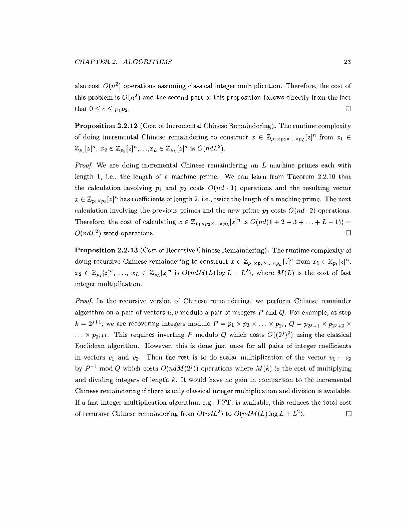
Proposition 2.2.12 (Cost of Incremental Chinese Remaindering). The runtime complexity
of doing incremental Chinese remaindering to construct x E Zplxp2x. . .xpL[z]n from xl E
Zpl [zIn, 5 2 E Zpz [zIn,. . . ,XL E ZpL [zIn is O(ndL2).
Proof. We are doing incremental Chinese remaindering on L machine primes each with
length 1, i.e., the length of a machine prime. We can learn from Theorem 2.2.10 that
the calculation involving pl and p2 costs O(nd . 1) operations and the resulting vector
x E Zpl xp2 [zIn has coefficients of length 2, i.e., twice the length of a machine prime. The next
calculation involving the previous primes and the new prime ps costs O ( n d . 2) operations.
Therefore, the cost of calculating x E ZPlxpzx . . . xpL[~]n is O(nd(1 + 2 + 3 + . . . + L - 1)) =
O ( n d ~ ~ ) word operations. 0
Proposition 2.2.13 (Cost of Recursive Chinese Remaindering). The runtime complexity of
doing recursive Chinese remaindering to construct x E ZP1 Xpz x . . .XpL [zIn from xl E Zpl [zIn,
x2 E Zp, [zIn, . . ., XL E ZpL [zIn is O(ndM(L) log L + L ~ ) , where M ( L ) is the cost of fast
integer multiplication.
Proof. In the recursive version of Chinese remaindering, we perform Chinese remainder
algorithm on a pair of vectors u, v modulo a pair of integers P and Q. For example, at step
k = 23", we are recovering integers modulo P = pl x p2 x . . . x p23 , Q = ~2~ x p23 +2 x
. . . x p2j+1. This requires inverting P modulo Q which costs 0 ( (2 j )2 ) using the classical
Euclidean algorithm. However, this is done just once for all pairs of integer coefficients
in vectors vl and v2. Then the rest is to do scalar multiplication of the vector vl - v2
by P-' mod Q which costs o ( n d ~ ( 2 j ) ) operations where M ( k ) is the cost of multiplying
and dividing integers of length k. It would have no gain in comparison to the incremental
Chinese remaindering if there is only classical integer multiplication and division is available.
If a fast integer multiplication algorithm, e.g., FFT, is available, this reduces the total cost
of recursive Chinese remaindering from O ( n d ~ ~ ) to O(ndM(L) log L + L ~ ) . 0
CHAPTER 2. ALGORITHMS 24
Runtime Complexity of Rational Reconstruction
Unlike all of the above procedures, rational number reconstruction tries to construct the
final answer and hence decide if we need more primes. Because we do not predict the
number of primes that are needed to successfully construct all coefficients in the solution
vector, we try rational reconstruction at certain points to test if we have used enough primes.
As a result, we have two parts which should be included in the total runtime complexity
of the rational reconstruction. We called them "unsuccessful rational reconstruction" for
the intermediate trials which return "FAIL", and "successful rational reconstruction" which
successfully returns the solution vector x E Q[z]/m(z). The same assumption is made here
that we will use L primes to successfully reconstruct the rational coefficients in the solution
vector.
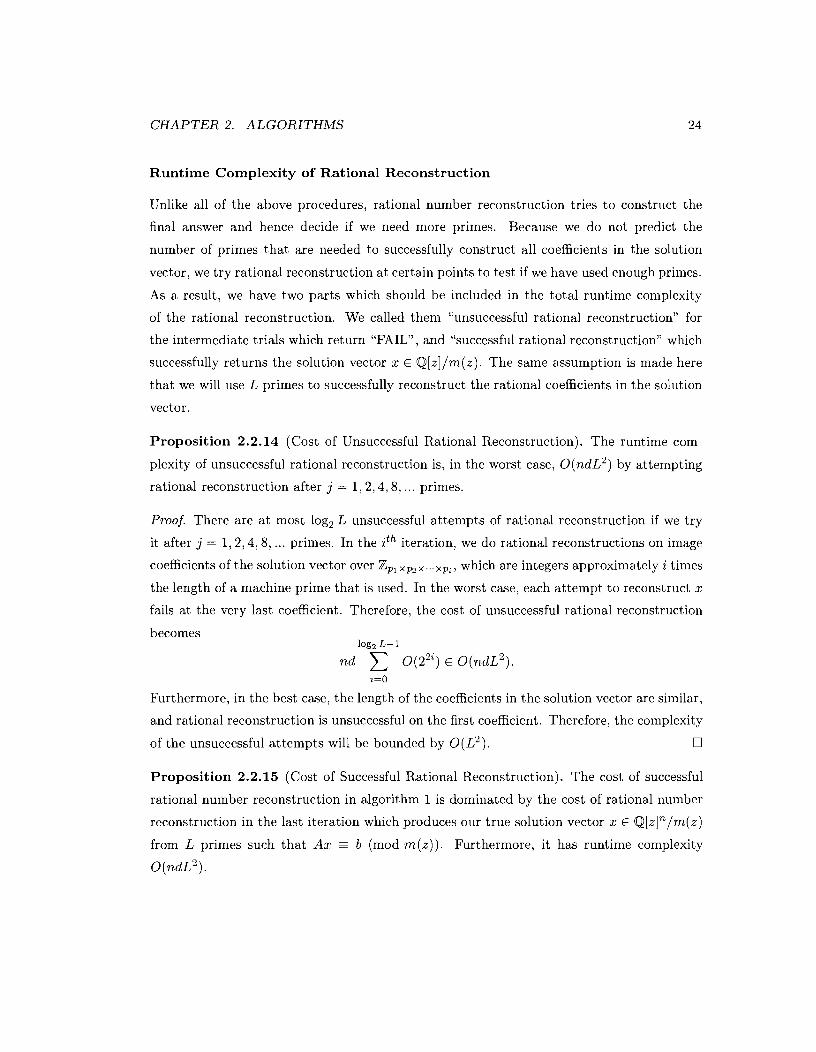
Proposition 2.2.14 (Cost of Unsuccessful Rational Reconstruction). The runtime com-
plexity of unsuccessful rational reconstruction is, in the worst case, O(ndL7 by attempting
rational reconstruction after j = 1,2 ,4 ,8 , ... primes.
Proof. There are at most logz L unsuccessful attempts of rational reconstruction if we try
it after j = 1,2 ,4 ,8 , ... primes. In the i th iteration, we do rational reconstructions on image
coefficients of the solution vector over Zp, xp2 ... xp,, which are integers approximately i times
the length of a machine prime that is used. In the worst case, each attempt to reconstruct x
fails at the very last coefficient. Therefore, the cost of unsuccessful rational reconstruction
becomes log, L- 1
nd 0 ( 2 ~ ? ) E 0(ndL2) . ?=O
Furthermore, in the best case, the length of the coefficients in the solution vector are similar,
and rational reconstruction is unsuccessful on the first coefficient. Therefore, the complexity
of the unsuccessful attempts will be bounded by 0 ( L 2 ) . 0
Proposition 2.2.15 (Cost of Successful Rational Reconstruction). The cost of successful
rational number reconstruction in algorithm 1 is dominated by the cost of rational number
reconstruction in the last iteration which produces our true solution vector x E Q[zIn/m(z)
from L primes such that Ax - b (mod m(z)) . Furthermore, it has runtime complexity
0 (ndL2) .

C H A P T E R 2. ALGORITHMS 25
Proof. Whenever the rational number reconstruction procedure produces a result x other
than "FAIL", it has successfully reconstructed all nd coefficients in the solution vector
x E Q[zIn/m(z). This vector x may or may not bc our truc solution vcct,or which satisfics
the equation Ax = b (mod m(z)) . The complexity of rational reconstruction is O ( N ~ ) , (see
section 1.4) where N is the length of the rational modulus m. Therefore, the cost of rational
reconstruction in the last iteration which produces our true solution vector x is 0(ndL2)
because each rational number reconstruction has to be done independently and the modulus
is the product of L machine primes. Since we perform the rational reconstruction in only the
lcth iterations, where lc = 2i, i E Z+ U {O), the cost of successful rational reconstructions is
~40" nd0(2~" E 0(ndL2) if we assume every attempt of rational number reconstruction
returns a vector x rather than "FAIL". Hence, the result follows. 0
Remark: The cost of the successful rational reconstruction of the 5 nd rational coeffi-
cients in x can similarly be reduced to roughly one rational reconstruction and O(nd) long
multiplications and divisions using a clever trick. Suppose we are reconstructing a rational
from an image ZL mod P and b is the LCM of the denominators of all rationals reconstructed
so far. The idea is to apply rational reconstruction to b x u mod P instead (see [2] for
details). Assuming fast integer multiplication and division are available, this improvement
effectively reduces the cost of rational reconstruction to that of fast multiplication, that is,
from 0(ndL2) to O(L2 + ndM(L)) where M(L) is the cost of multiplication of integers of
length L and the L2 term is the cost of the classical Euclidean algorithm which we use for
computing inverses and rational reconstruction.
Proposition 2.2.16. Checking if m(z)lAx - b takes 0(n2d2cL) operations.
Proof. This checking irivolvcs a matrix vcctor multiplicatiori of polyriorriials with coefficient
lengths c and L, which costs O(n2d2cL). This cost dominates the cost of other operations
in this checking procedure. 0
Theorem 2.2.17. The running time complexity of the Chinese remaindering approach is
O(n3dL + n2d2cL + ndL2).
Remark: The complexity of the checking procedure seems to dominate the cost of all pro-
cedures in Algorithm 1 except the Gaussian elimination, Chinese remaindering, and rational
reconstruction. However, in practice, we inip~uvc its eficiericy by clearing all fractions in x

CHAPTER 2. ALGORITHMS 26
before the matrix vector multiplication, and observed its cost never exceed 10% of the total
running time.
2.2.5 Run Out of Primes Problem on 32 bit Machines
Lemma 2.2.2 says we will have lots of primes to use. However, in an early implementation
where we chose 16 bit or smaller machine primes on a 32 bit machine, the following problem
arose. If we choose the l l th cyclotomic polynomial
to be our minimal polynomial, and a matrix A E ~ [ z ] ~ ~ ~ ~ ~ / m ( z ) , vector b E ~ [ z ] ~ O / m ( z )
with random 3 decimal digit coefficients to be our input, we ran out of primes since the solu-
tion vector x would be a vector of polynomials with coefficient length about 3672 decimal dig-
its long. Only 1 in 11 primes can be used (lemma 2.2.1). If we start with p r e ~ p r i r n e ( 2 ~ 1 6 ) ,
i.e., the largest 16 bit prime, and m(z) = cPll(z), the product of all usable primes is 2801
decimal digits long which can only recover fractions with size approximately 2800 decimal
digits long. To solve this problem, we use 25 bit floating point primes on 32 bit machines
which is supported by Maple.
2.3 Linear p-adic Lifting Approach
2.3.1 Description
The linear pad ic lifting approach is based on developing an integer u in its padic represen-
tation: 2
'U. = 'ZLO + + u2p + ' ' ' + 'ZLkp k
where p is an odd positive prime, k is such that pktl > 21ul, and ui E Zp(O < i < k)
Consider the polynomial
and let p and k be chosen such that pktl > 2umax, where umax = max, IueI If each integer
coefficient ue is expressed in its pad ic representation
CHAPTER 2. ALGORITHMS
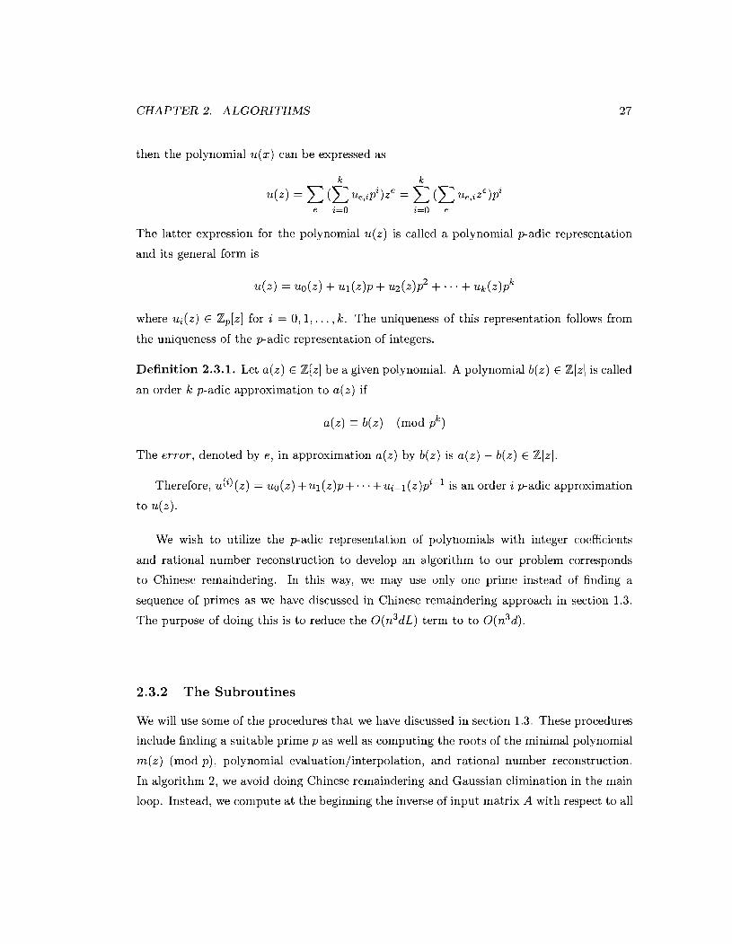
then the polynomial u(x) can be expressed as
The latter expression for the polynomial u(z) is called a polynomial padic representation
and its general form is
where ui(z) E Zp[z] for i = 0,1, . . . , k. The uniqueness of this representation follows from
the uniqueness of the padic representation of integers.
Definition 2.3.1. Let a(z) E Z[z] be a given polynomial. A polynomial b(z) E Z[z] is called
an order k p-adic approximation to a(z) if
a(z) - b(z) (mod pk)
The error, denoted by e, in approximation a(z) by b(z) is a(z) - b(z) E Z[z].
Therefore, u ( ~ ) ( z ) = uo(z) + ul (z)p + . . . + ui-1 (z)pi-l is an order i padic approximation
to u(z).
We wish to utilize the pa.dic representation of polynomials with irit3eger c:oeffic:ioiits
and rational number reconstruction to develop an algorithm to our problem corresponds
to Chincsc rcrnai~idering. In this way, wc may use only one prime instead of finding a
sequence of primes as we have discussed in Chinese remaindering approach in section 1.3.
The purpose of doing this is to reduce the 0 ( n 3 d ~ ) term to to 0(n3d).
2.3.2 The Subroutines
We will use some of the procedures that we have discussed in section 1.3. These procedures
include finding a suitable prime p as well as computing the roots of the minimal polynomial
m(z) (mod p), polynomial evaluation/interpolation, and rational number reconstruction.
In algorithm 2, we avoid doing Chinese remaindering and Gaussian elimination in the main
loop. Instead, we compute at the beginning the inverse of input matrix A with respect to all

C H A P T E R 2. ALGORITHMS
Figure 2.2: Process flow of the linear padic lifting approach
the roots of m(z) (mod p) and cache them for further computation. In the classical padic
lifting approach that we discussed in section 1.5, we compute the order Ic + 1 approximation
from the order Ic approximation, and keep updating the error term in each iteration until
the error term becomes zero. In this problem, we are not able to make the error term zero
since the solution vector x may contain fractions. By doing modulo operations mod pk, we
will not be able to get a zero error term unless p is a divisor of the numerator. Therefore,
we cannot determine the stopping criteria by just checking if the error goes to zero. So, we
must periodically reconstruct x(lC) E Q[zIn mod pk using rational reconstruction, and stop
when Ax - b mod m(z) holds.
Computing the Inverse of Input Matrix A (mod p)
In algorithm 2, we will need to compute the images of solution vector x by the equation
A(cui)x(cui) - e(cui) (mod p), where e denotes the updated error term in each iteration. The
initial value of e is our input vector b. Its value is updated in each iteration while the input
matrix A and the prime p stay the same over all iterations of computation. Therefore, we
compute the inverse of A(cri) in advance so that we just perform matrix vector multiplication
in each iteration instead of Gaussian elimination in the main loop. This is the main gain of p
adic lifting over Chinese remaindering. To further reduce the complexity, we use polynomial
evaluation to reduce computation to modp and then interpolate the polynomials afterward.
Therefore, we will need the inverses of A(ai) (mod p) over all the roots a1, a 2 , . . . , ad of

C H A P T E R 2. A L G O R I T H M S 2 9
m(z) (mod p). We achieve this in three steps: first reduce the coefficients in A by p; then
substitute z by the roots; and lastly compute the inverse of the matrices obtained from
the previous subroutine. Gaussian elimination costs 0 ( n 3 ) operations over Z, to compute
A ( U ~ .
Updating the Error Term
Similar t o the classical pad ic lifting algorithms, we need t o update the error term in each
iteration. This procedure is simply written as ek+l = (ek - Axk mod m(z)) /p. In section
2.3.4, we use this formula for updating the error term. However, it turns out to be inefficient
if we use the straight forward computation. We give two efficient algorithms for updating
ek+l in section 2.3.5.
Updating the Image Solution Vector
We need to update the image solution vector xktl in the kth lifting step before we can
use it for rational reconstruction. Similar to the Chinese remainder algorithm that we have
discussed in section 2.2.4, we may use either incremental or recursive algorithms for updating
the image solution vectors.
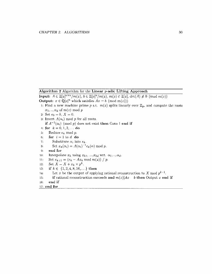
2.3.3 The Algorithm
2.3.4 Runtime Analysis of Algorithm 2
We state the running time of Algorithm 2 in terms of n , dl C, and L, the number of lifting
steps that Algorithm 2 takes. For pL to be large enough to reconstruct rationals of in x ,
L E O(log 11~1103)~
Proposition 2.3.2. Invert matrix A over all the roots modulo the machine prime p takes
0 ( n 3 d + n2dc + n2d2) operations.
Proof. Assuming we have obtained the roots all a 2 , . . . , a d of m(z ) (mod p), we will need to
find A-'(u1), ~ - l ( a ~ ) , . . . , A-'(CX~) E ZFxn. AS we ha.ve described in section 2.2.4, we first
rcduce the cocfficicnts in the input ma.trix A and then perform the evaluations and calculate
thc inverses. Thc coefficicnt reduction stcp takas 0(n2dc) operations (Proposition 2.2.6),
and evaluation step takes 0 ( n 2 d 2 ) operations (Proposition 2.2.7). The computation of
CHAPTER 2. ALGORITHMS
Algorithm 2 Algorithm for the Linear padic Lifting Approach Input: A E Z [ z I n x n / m ( z ) , b E Z [ z I n / m ( z ) , m ( z ) E Z [ z ] , det(A) $ 0 (mod m ( z ) ) Output: x E QlzIn which satisfies A x = b (mod m ( z ) ) ) . . . . .
Find a new machine prime p s.t. m ( z ) splits linearly over Z,, and compute the roots a1 , . . , a d of m ( z ) mod p Set eo = b, X = 0. Invert A(ai) mod p for all roots. if AP1(ai) (mod p) does not exist then Goto 1 end if for k = 0 , 1 , 2 , . . . do
Reduce ek mod p. for i = 1 to d do
Substitute ai into ek. Set x k ( a i ) = A(a i ) - ' e k (a ) mod p.
end for Interpolate xr, using xk l , ..., xkd wrt. al , . . ,ad. Set ek+l = (ek - A x k mod m ( z ) ) / p. Set X = X + xk x pk .
if k E { l , 2 , 4 , 8 , 1 6 , . . .) then Let x be the output of applying rational reconstruction to X mod pk+l. if rational reconstruction succeeds and m ( z ) l A x - b then Output x end if
end if
C H A P T E R 2. ALGORITHMS 31
inverting the matrices over ZFxn costs no more than d times the cost of Gaussian elimination
therefore has complexity O(n3d). Therefore, its total runtime complexity becomes O(n3d + n2dc + n2d2). 0
Before we determine the cost of computing the error ek+l in step 11, we show that I lekl l w is bounded.
Lemma 2.3.3. Let m(z) = zd + ~ , d ~ i ajzi with ai E Z. Let f (z) = ~ f = ~ bizi with bi E Z.
Let r be the remainder of f divided m. Then r E Z[x] (because m is monic) and llrllm 5
(1 + llm11,)611 f 11, where 6 = 1 - d + 1.
Proof. The quotient of f divided m has degree 1 - d, hence, there are at most 1 - d + 1 = 6
subtractions in the division algorithm. The first subtraction is f l := f - blxl-dm. We have
llblmllw I I l f llmllmllm, hence,
For the purpose of bounding Ilrllm we assume deg f l = 1 - 1. The next subtraction is
f2 := f l - l ~ ( f ~ ) x l - l - ~ m. Bounding Ilc(fl)l 5 1 1 flllw we have
Repeating this argument the result is obtained. 0
Theorem 2.3.4. Let ek be the error term in the kth iteration of Algorithm 2. The absolute
value of the integer coefficients in ek is bounded by I lekII, I 1 /[Alb] /l,nd(l + I~ntl
Proof. Given the formula ek+l = '*-Fk, the initial value eo = b, and IIxkll-. < p for all
k E Z. Let c be the bit length of the maximum of the absolute value of the coefficients in
the input matrix A and vector b, i.e., c = log, max(llAllm, l\bllm). We consider firstly the
coefficients in el = ' o - ~ " Q . The matrix vector multiplication Axo would produce maximum P
coefficient I IAI I m (p - 1)nd. After reducing the polynomials by m(z) , the maximum possible
coefficient in Axo mod m(z) is bounded by
by lemma 2.3.3. After subtracting by by eo and dividing by p, we know the maximum
coefficient in el is bounded by 2'nd(l + Ilmllm)d-l. Induction Hypothesis: Assume that
CHAPTER 2. ALGORITHMS
Ilekll, is bounded by 2'nd(l + I(mll,)d-l. NOW we know that
for every k E Z. Therefore, we know the bit length of the integer coefficients in ek is
which is bounded by O(c + d) assuming llmll, is a constant that is smaller than our base
B and also B > nd. 0
Proposition 2.3.5. The runtime complexity of solving the system Axk - ek (mod p) for
xk is O(n2d + d2) using the precomputed inverses of A(ai ) , 1 5 i 5 d, obtained from
Algorithm 3.
Proof. First of all, we reduce the coefficient of ek modulo p, and then do the polynomial
evaluations over the roots. The reduction step takes O(c + d) operations because the length
of the coefficients in ek is bounded by O(c + d), and p is a fixed size machine prime. Each
polynomial evaluation takes O(d) operations, and each system solving of A(cri)xk(a,) = ek(cr,) (mod p), for xk(a i ) takes 0 ( n 2 ) operations since ~ - l ( a ~ ) ' s have been previously
computed. The last step is to do polynomial interpolation to construct xk E Zp[zIn which
costs O(nd2) operations. Therefore, the runtime complexity of solving the system Axk - ek (mod p) for xk in the k t h iteration is O(n2d + nd2). 0
Proposition 2.3.6. Updating the error term takes 0(n2d2c) operations in each iteration
assuming classical polynomial multiplication and division are used for Axk mod m(z).
Proof. Theorem 2.3.4 gives us an upper bound of the coefficients in the error terms ek.
Therefore, we know that the coefficients in ek do not grow over the iterations. To update
the error term ek+l in the kth iteration, we need to do a matrix vector multiplication
of polynomials over Z then divide by m(a). Assuming [Im(z)l l c o is constant, the matrix
vector multiplication costs 0 ( n 2 ) operations, and the polynomial multiplications contribute
another 0(d2c) factor since the coefficient length in A is bounded by c. The cost of updating
the error term is dominated by the above matrix vector multiplication, which is 0(n2d2c).
0
CHAPTER 2. ALGORITHMS 33
Note, In section 2.3.5, two approaches other than classical polynomial multiplication of A
and xk over the polynomials are introduced which reduce the runtime complexity of updating
the error term.
Proposition 2.3.7. The runtime complexity of updating the image solution vectors x ( ~ ) is
0 ( n d L 2 ) if we update the solution vector incrementally, and O ( n d M ( L ) log L ) if we update
the solution vector recursively, where M ( L ) is the cost of multiplying integers of length L.
Proof. Similar to the Chinese remaindering procedure that we have discussed in section
2.2.4, updating the image solutions incrementally causes multiplications between small
integers, c.g., cocfficicrits of xk E ZP[zln, and big integers, e.g., pk, in each iteration.
Therefore, faster integer multiplication algorithms do not apply. As a result, the com-
plexity of incremental updating becomes ~ f = ~ ndi E O(ndL2) . In the case of recursive
updating, we update the solution vector xk as follows: xo + xlp + x2p2 + . . . + xkPk = k - 1
) + p 5 ( x q + X ~ + ~ ~ + X I p2+. . .+xkP5) . There are logL 2 +2
levels of recursion, and in the ith recursion, the cost is o ( ~ ~ M ( $ ) L ) E O ( n d M ( L ) ) where
M ( L ) is the cost of fast integer multiplication which is usually M ( N ) = N log N log log N .
Therefore, the runtime complexity becomes O ( n d M ( L ) log L ) if it is done using fast integer
multiplication, e.g. FFT for big integer multiplication. 0
Theorem 2.3.8. The total running time of the padic lifting approach is O(n3d+n2d2cL+
ndL2) if we use classical polynomial and integer algorithms.
The first contribution, n3d, is the cost of the d matrix inversions. The second, n2d2cL, is
the total cost of computing the error terms ek and the trial division m(z) lAx - b. The third,
ndL2, is the cost of converting the solution vector to integer polynomial representation from
its padic representation.
Proof. In this algorithm, we only need one prime p such that the minimal polynomial splits
linearly over Z,. The time for computing this can be ignored. In step 3, we pre-compute the
inverse of the matrix A at each root modulo p using Gaussian elimination. This costs 0 ( n 3 d )
arithmetic operations in total. Step 5 costs O(ndcL + nd2L) operations since ek is a vector
of polynomials of degree < d with coefficient length in O(c + d ) and is done for L iterations.
The substitution of all d roots into ek costs 0 ( n d 2 L ) operations. Computing the solution
vector x k ( a i ) is just a matrix vector multiplication modulo p which costs 0 ( n 2 d L ) in total.
Interpolation costs 0 ( n d 2 L ) which is the same as in algorithm 1. To compute the error ek
CHAPTER 2. ALGORITHMS 34
in step 11, we should do a matrix vector multiplication of polynomials over Z then divide by
m(z). The cost is dominated by this computation which is O(n2d2cL) operations since fast
integer multiplication is not applicable here when using classical polynomial multiplication.
The cost of adding xkpk to X is 0 ( n d ~ ~ ) which is the same cost as rational reconstruction
in both algorithms 1 and 2. Trial division in step 15 costs O(n2d2cL) operations which is
the same cost of computing the error term. Therefore, the total running time for algorithm
2 is 0 (n3d + n2d2cL + n d ~ ~ ) . 0
2.3.5 Computing the Error Term
In our implementation of Algorithm 2, the most expensive component is the computation
of the error term in step 11. In particular, the matrix vector multiplication Axk needs
to be computed over Z. This requires n2 polynomial multiplications. Assuming classical
polynomial multiplication and integer multiplication, it has complexity 0(n2d2c) for each
iteration. We consider two approaches which theoretically reduce the runtime complexity
by a factor of d.
Without loss of generality, let C = Ax mod m(z) E Z[zIn, where x represents xk in the
kth iteration. From Theorem 2.3.4, we learn that 1 lCl loo 5 ndpl l ~ l l ~ ( l + 1 lml We dis-
cuss below two approaches, namely "pre-CRT" and "Single-Point Evaluation/Interpolation" , to reduce the complexity of computing C . Note that, since the length of the vector C is
more than 0(n2dc) in general, we may not expect to reduce the complexity of computing
the error term by more than a factor of d.
The pre-CRT Approach of Computing Axk
As we have tried in section 2.2, we can transfer the operations over polynomials into the
computations over integers mod p, hence reduce the complexity. To compute C = Ax mod
m(z), We pick a sequence of machine primes pl, p2, p3,. . . such that m(z) splits into distinct
linear factors over Zp,. For each prime pi, we find the roots crl, ~ 2 , . . . , cud of m(z) mod pi
and substitute them into A and x, then interpolate over z from A(cri)x(cri), cri to obtain
Ci E ZpZ[zln. After we apply the above procedure for sufficiently many primes, we can
use the Chinese remainder algorithm to obtain C E Zp,xp,xp,,...[z]n, which is the same as
C E Z [ ~ ] ~ / m ( z ) . For example, let aj be one of the d roots of m(z) (mod p,). We compute
Ci(aJ) = A(ffj)xk(ffj) mod pi for all d roots, hence obtain Ci E Zpi[z] by interpolating the
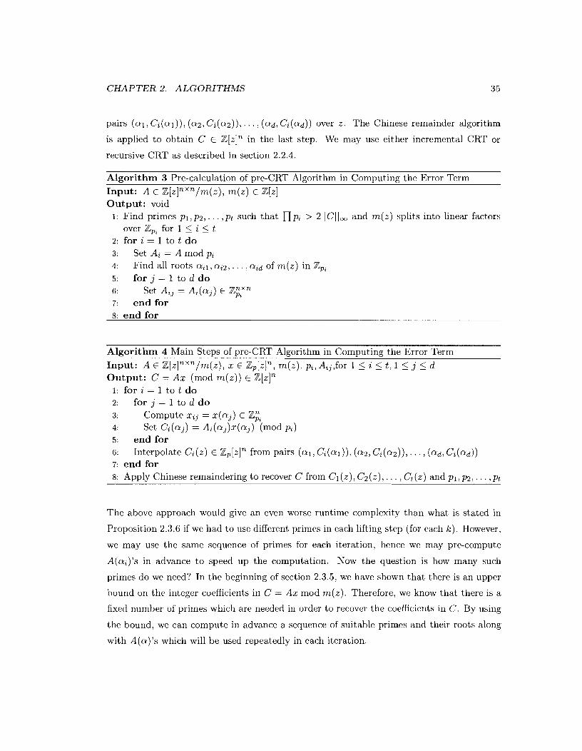
C H A P T E R 2. ALGORITHMS 3 5
pairs ( a l , Ci(a l ) ) , (a2, Ci(a2)) , . . . , ( ad , Ci (ad)) over z . The Chinese remainder algorithm
is applied to obtain C E Z[zIn in the last step. We may use either incremental CRT or
recursive CRT as described in section 2.2.4.
Algorithm 3 Pre-calculation of pre-CRT Alnorithm in Computinn the Error Term Input: A E Z[zInxn/m(z), m(z) E Z[z] Output: void
1: Find primes p l , p2,. . . ,pt such that n p i > 211Cllm and m(z) splits into linear factors over Zpl for 1 5 i 5 t
2: for i = 1 to t do 3: Set Ai = A mod pi 4: Find all roots Qil, a iz , . . . , a i d of m(z) in Zpi 5: for j = 1 to d do 6: Set Aij = A,(aj) E q X n
7: end for
Algorithm 4 Main Steps of pre-CRT Algorithm in Computing the Error Term Input: A E Z[zInxn/m(z), x E Zp[zIn, m(z) , pi,Aij,for 1 5 i 5 t , 1 5 j 5 d Output: C = Ax (mod m(z ) ) E Z[zIn
1: for i = 1 to t do 2: for j = 1 to d do 3: Compute xij = x ( q ) E ZFt 4: Set Ci (a j ) = Ai(a j )x(a j ) (mod pi) 5: end for 6: Interpolate Ci(z) E ZP[zln from pairs ( a i , Ci (a i ) ) , ( ~ 2 , Ci(a2)), . . . , ( a d , Ci(ad)) 7: end for 8: Apply Chinese remaindering to recover C from Cl (z) , C2 (z) , . . . , Ct (z) and pl , pz , . . . , pt
The above approach would give an even worse runtime complexity than what is stated in
Proposition 2.3.6 if we had to use diffcrcnt primes in each lifting step (for ea.ch I ; ) . However,
we may use the same sequence of primes for each iteration, hence we may pre-compute
A(cri)'s in advance to speed up the computation. Now the question is how many such
primes do we need? In the beginning of section 2.3.5, we have shown that there is an upper
t)ound on the integer coefficients in C = Ax mod m(z) . Therefore, we know that there is a
fixed nurnber of primes which are needed in order to recover the coefficierits in C . By using
the bound, we can compute in advance a sequence of suitable primes and their roots along
with A((Y)'s which will be used repeatedly in each iteration.
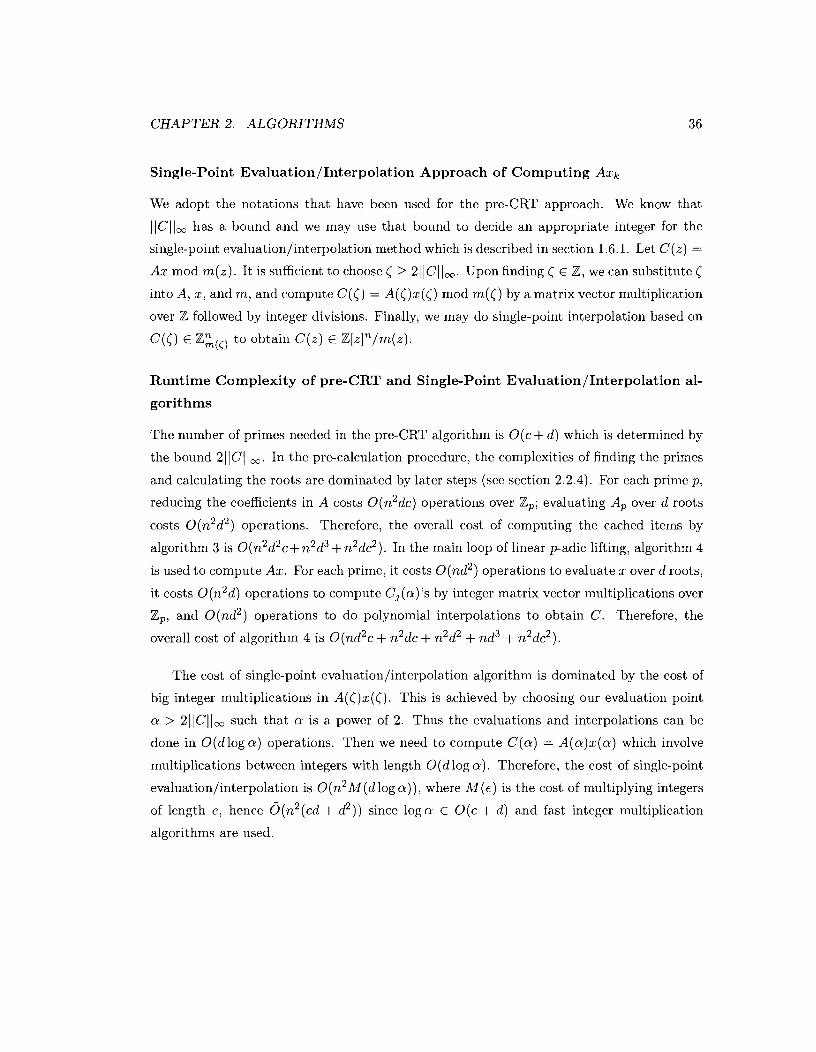
CHAPTER 2. ALGORITHMS 36
Single-Point Evaluation/Interpolation Approach of Computing Axk
We adopt the notations that have been used for the pre-CRT approach. We know that
llCllw has a bound and we may use that bound to decide an appropriate integer for the
single-point evaluation/interpolation method which is described in section 1.6.1. Let C(z) =
Ax mod m(z). It is sufficient to choose < > 211Cllm. Upon finding < E Z, we can substitute < into A, x , and m, and compute C(<) = A(<)x(<) mod m(<) by a matrix vector multiplication
over Z followed by integer divisions. Finally, we may do single-point interpolation based on
C(<) E Zz(C) to obtain C(z) E Z[zIn/m(z).
Runtime Complexity of pre-CRT and Single-Point Evaluation/Interpolation al-
gorithms
The number of primes needed in the pre-CRT algorithm is O(c + d) which is determined by
the bound 211Cllw. In the pre-calculation procedure, the complexities of finding the primes
and calculating the roots are dominated by later steps (see section 2.2.4). For each prime p,
reducing the coefficients in A costs 0(n2dc) operations over Zp; evaluating Ap over d roots
costs 0 (n2d2) operations. Therefore, the overall cost of computing the cached items by
algorithm 3 is 0(n2d2c+ n2d3 + n2dc2). In the main loop of linear padic lifting, algorithm 4
is used to compute Ax. For each prime, it costs 0 (nd2) operations to evaluate x over d roots,
it costs 0 (n2d) operations to compute Cj(a) 's by integer matrix vector multiplications over
Z,, and 0 (nd2) operations to do polynomial interpolations to obtain C. Therefore, the
overall cost of algorithm 4 is O(nd2c + n2dc + n2d2 + nd3 + n2dc2).
The cost of single-point evaluation/interpolation algorithm is dominated by the cost of
big integer multiplications in A(<)x(<). This is achieved by choosing our evaluation point
a > 211Cllw such that a is a power of 2. Thus the evaluations and interpolations can be
done in O(d log a ) operations. Then we need to compute C ( a ) = A(a)x(a ) which involve
multiplications between integers with length O(d log a ) . Therefore, the cost of single-point
evaluation/interpolation is 0 ( n 2 ~ ( d l o g a ) ) , where M(e) is the cost of multiplying integers
of length e, hence 0(n2(cd + d2)) since log a E O(c + d) and fast integer multiplication
algorithms are used.
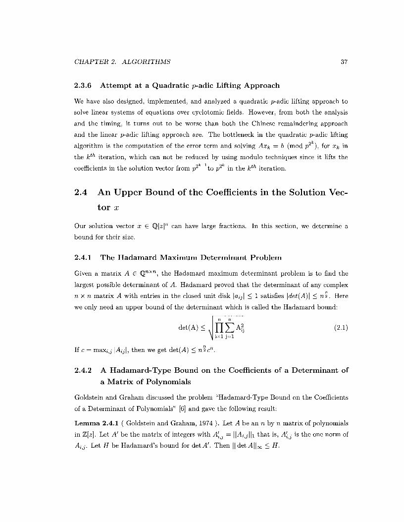
C H A P T E R 2. ALGORITHMS 3 7
2.3.6 Attempt at a Quadratic padic Lifting Approach
We have also designed, implemented, and analyzed a quadratic padic lifting approach to
solve linear systems of equations over cyclotomic fields. However, from both the analysis
and the timing, it turns out to be worse than both the Chinese remaindering approach
and the linear padic lifting approach are. The bottleneck in the quadratic padic lifting
algorithm is the computation of the error term and solving Axk = b (mod p 2 k ) , for xk in
the kth iteration, which can not be reduced by using modulo techniques since it lifts the
coefficients in the solution vector from p2kp1to p2k in the kth iteration.
2.4 An Upper Bound of the Coefficients in the Solution Vec-
tor x
Our solution vector x E Q[zIn can have large fractions. In this section, we determine a
bound for their size.
2.4.1 The Hadamard Maximum Determinant Problem
Given a matrix A E Qnxn, the Hadamard maximum determinant problem is to find the
largest possible determinant of A. Hadamard proved that the determinant of any complex
n x n matrix A with entries in the closed unit disk laiJ[ 5 1 satisfies Idet(A)I 5 nz . Here
we only need an upper bound of the determinant which is called the Hadamard bound:
If c = maxi,j IAijl, then we get det(A) 5 nz cn.
2.4.2 A Hadamard-Type Bound on the Coefficients of a Determinant of
a Matrix of Polynomials
Goldstein and Graham discussed the problem "Hadamard-Type Bound on the Coefficients
of a Determinant of Polynomials" [6] and gave the following result:
Lemma 2.4.1 ( Goldstein and Graham, 1974 ). Let A be an n by n matrix of polynomials
in Z[z]. Let A' be the matrix of integers with Aij = IIAi,jlll that is, is the one norm of
Ai,j. Let H be Hadamard's bound for det A'. Then I I det A1 1, < H.
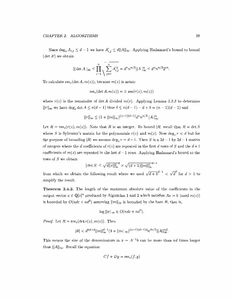
CHAPTER 2. ALGORITHMS 38
Since deg, Ai,J < d - 1 we have A& < dl/AllW. Applying Hadamard's bound to bound
I det A'I we obtain
To calculate res,(det A, m(z ) ) , because m(z) is monic
where r (z) is the remainder of det A divided m(z). Applying Lemma 2.3.3 to determine
llrlloo we have deg,detA < n ( d - 1) thus b 5 n ( d - 1) - d + 1 = ( n - l ) ( d - 1) and
Let R = res,(r(z), m(z)). Note that R is an integer. To bound IRI recall that R = det S
where S is Sylvester's matrix for the polynomials r (z) and m(z). Now deg, r < d but for
the purpose of bounding IRI we assume deg, r = d - 1. Then S is a 2d - 1 by 2d - 1 matrix
of integers where the d coefficients of r(z) are repeated in the first d rows of S and the d + 1
coefficients of m(z) are repeated in the last d - 1 rows. Applying Hadamard's bound to the
rows of S we obtain
from which we obtain the following result where we used md-' < &d for d > 1 to
simplify the result.
Theorem 2.4.2. The length of the maximum absolute value of the coefficients in the
output vector x E Q[zIn produced by Algorithm 1 and 2 which satisfies Ax = b (mod m(z))
is bounded by O(ndc + nd2) assuming llmlloo is bounded by the base B, that is,
log IIxlloo E O(ndc+ nd2).
Proof. Let R = res,(det r ( z ) , m(z)) . Then
This means the size of the denominators in x = A-'b can be more than nd times longer
than IIAllW. Recall the equation

CHAPTER 2. ALGORITHMS 39
where C and D are polynomials with integer coefficients and deg C < degg, deg D < deg f .
We replace f by m(z) , and replace g by det A then get that D/res,(f,g) is the inverse of
det A mod m(z) . Bccausc of the fact that the integer coefficients in D can be found among
the determinants of the minors of Sylvester matrix Syl,(r(z), m(z) ) , we can obtain an upper
bound for IIDllm, that is,
By Cramer's rule, we know that
det A ( ~ ) xi = - mod m(z).
det A
Since we have assumed that c = log2 max(llAIl,, Ilbllm), we can use the bound we obtained
for det A mod m(z) to bound di) = det A(" mod m(z) , that is,
The last step is to obtain xi = di)g mod m(z) = ( T ( ~ ) D mod m(z ) ) /R from which we can
obtain the bound D
IIxxIm 5 (1 + l l ~ l l m ) d ~ l d l l ~ ( i ) m ~ l l m ~
Hence, we can now conclude that log 11x1 1, E O(ndc+ nd2) because log I ~ r ( ~ ) l ~ , is in O(nd+
nc) and log I I 11, is in O(ndc + nd2) and the rest terms are dominated by these terms for
i from 1 to 12. 0
This bound may be used to bound the number of primes needed in Algorithm 1, and the
number of lifting steps in Algorithm 2 to output x while the input is a non-singular system.
However, in our experiments on systems given by Vahid Dabbaghian (Table 2.2,2.3), the
number of primes (lifting steps) used are much smaller than the bound.
2.5 Runtime Complexity Comparison
We have shown that the runtime complexity of the Chinese remaindering approach is TCTt =
0(n3dL + n2d2cL + ndL2) where L is the number of machine primes used, and the runtime
complexity of the pad ic lifting approach is zift = 0(n3d + n2d2cL + ndL2) where L is the
number of lifting steps. In section 2.4 we showed for llmllm < B that L E O(ndc + nd2).
We may now compare the runtime complexities of Algorithm 1 and 2 just in terms of the
CHAPTER 2. ALGORITHMS 40
variables n, d, and c in the input. Therefore, TcTt becomes O(n4d2c + n3d3c2 + n4d3 + n3d4c + n3d5), and q,ft becomes O(n%Q2 + n3d4c + n3d5). The n4d2c and n4d3 terms
in TcTt are contributed by the Gaussian eliminations over Zp . The n3d3c2, n3d4c and n3d5
terms are contributed by the rational reconstruction and trial division of m(z)lAx - b in
both Algorithm 1 and 2, and it also represents the contribution by updating the error terms
and adding up the image solution vectors in Algorithm 2.
The pre-CRT and single-point evaluation/interpolation algorithms are used in Algorithm
2 to improve the complexity of computing the error term. However, they do not change the
overall complexity of Algorithm 2 even though we observe a better running time in tables
2.1, 2.2, and 2.3. Fast algorithms are used to do Chinese remaindering in Algorithm 1,
adding up the image solution vectors in Algorithm 2, and rational reconstructions in both
algorithms. However, they do not change the runtime complexity of either Algorithm 1 or
Algorithm 2.
2.6 Implementation and Timings
We have implemented Algorithms 1 and 2 in Maple 10. Both of the algorithms are output
sensitive. In our programs, we used the Maple library routines i r a t r e c o n for rational
number reconstruction, and our own routine i scyclo tomic to find the order k of the given
cyclotomic polynomial. We used the library routine Roots(m) mod p to find the roots of
m(z) in Z,. We use 25 bit floating point primes on 32 bit machines, and 31 bit integer
primes on 64 bit machines. If we choose the primes as stated, we can take advantage of
the fast C code in the LinearAlgebra: -Modular package which provides fast polynomial
evaluation, linear solving and matrix inversion over Z,. We implemented the recursive
versions of Chinese remainder algorithm and updating the solution vectors in the linear
padic lifting approach where we use pre-CRT to compute the error terms.
2.6.1 Timing the Random Systems and Real Systems
We chose a set of randomly generated systems and two sets of real systems given by Dr.
Vahid Dabbaghian-Abdoly for our benchmarks. All timings we give in the following were
obtained using Maple 10 on an AMD@ Opteron 150 processor @ 2.4 GHz with 12GB of
RAM. Our programs are designed for dense inputs. They do not take advantage of any
C H A P T E R 2. ALGORITHMS
structure if the input systems are sparse.
Data Set 1:
For the first data set we use the 7th cyclotomic polynomial m(z) = 1 + z + z2 + z3 + z4 + z5 + z6 as the minimal polynomial. The first data set consists of systems of dimension
5,10,20,40,80,160 where the entries of A and b were generated using the Maple command
for different values of c which specifies the lengths of the integer coefficients in binary
digits. This Maple command outputs a dense polynomial in z with degree 5 and coefficients
uniformly chosen a t random from [O,2').
Table 2.1 shows the running time of dense random polynomial inputs for both of our
algorithms, namely "CRT" and "Lift". In addition, the pre-CRT and single-point evalu-
ationlinterpolation algorithms embedded in the linear padic lifting algorithm are timed,
namely "Liftl" and "Lift2". We timed Gaussian elimination, namely "GE", as a comple-
ment by using an optimized version of Gaussian elimination written in Maple by Dr. Michael
Monagan. This procedure gives a much better running time than the Maple Linearsolve
procedure even though they both use Gaussian elimination hence with same complexity. We
observe that either of our improved linear padic lifting approaches are much faster than the
Chinese remaindering approach when the dimension n of the input matrix and input vector
gets larger, and our modular algorithms beats Gaussian elimination when the dimension of
the matrix is bigger than 20.
Remark: In all of our timings, we write the runtime in CPU seconds.
Data Set 2:
The problems in this data set were given to us by Vahid Dabbaghian. They include systems
with various dimensions, coefficient lengths, and minimal polynomials. The systems are
available a t
Table 2.2 and Table 2.3 show the running times for the systems given to us by Vahid
Dabbaghian. The labeling of the algorithms is the same as in Table 2.1. In addition, we
CHAPTER 2. ALGORITHMS
show here the number of machine primes that are needed to construct the solution vector in
the Chinese remaindering approach. This corresponds to the number of lifting steps needed
in the linear padic lifting algorithms. One can see that the modular algorithms are much
faster than Gaussian elimination.

C H A P T E R 2. ALGORITHMS
Coefficient length c in binarv d i d 11 Remark 10241 7.396 GE 31.30 CRT 85.79 Lift1 19.84 Lift2 19.15 Lift 93.62 GE 158.8 CRT 306.5 Lift 1 96.57 Lift2 118.4 Lift 1507 GE 930.3 CRT 1236 Lift1 584.8 Lift2 827.4 Lift - GE - CRT - Lift 1
4047 Lift2 - Lift
Lift 1 Lift2 Lift
Liftl Lift2 Lift
Table 2.1: Runtime (in CPU seconds) of Random dense input with various dimensions and coefficients. "-" denotes the running time is over 5,000 seconds.
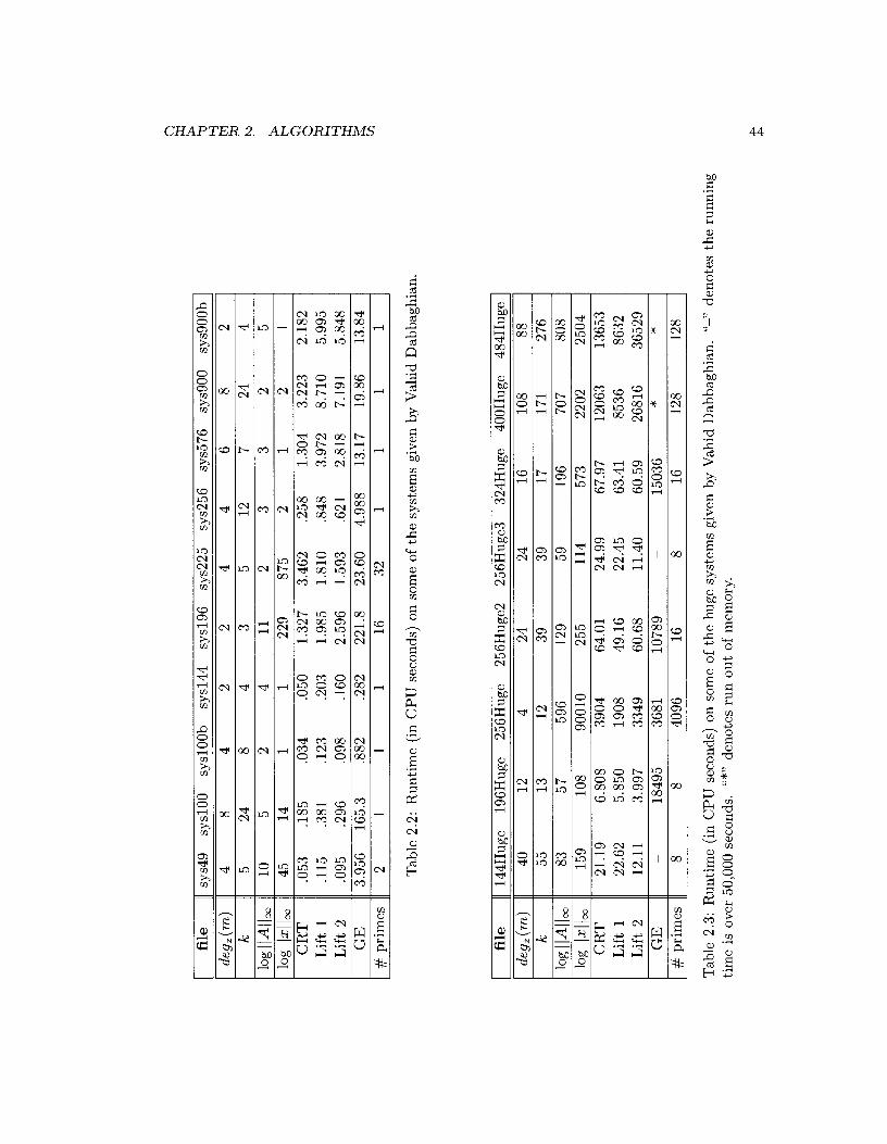
file
11 s
ys49
sy
slO
O
sysl
OO
b sy
s144
sy
s196
sy
s225
sy
s256
sy
s576
sy
s900
sy
s900
b ]
I # p
rim
es 11
2
I I
1
1
1
16
32
1
1
1
1
1%
IlAllo
o 10
gIIx
IIm
C
RT
L
ift
1
Lif
t 2
GE
Tab
le 2
.2:
Run
tim
e (i
n C
PU
sec
onds
) on
som
e of
th
e sy
stem
s gi
ven
by V
ahid
Dab
bagh
ian.
10
5 2
4 11
2
3 3
2 5
45
14
1
1
229
875
2 1
2 1
.053
.I
85
,0
34
,050
1.
327
3.46
2 .2
58
1.30
4 3.
223
2.18
2 .I
15
.3
81
.I2
3
.203
1.
985
1.81
0 .8
48
3.97
2 8.
710
5.99
5 .0
95
.296
,0
98
,160
2.
596
1.59
3 .6
21
2.81
8 7.
191
5.84
8 3.
956
165.
3 ,8
82
.282
22
1.8
23.6
0 4.
988
13.1
7 19
.86
13.8
4
file
d
eo,(
m)
144H
uge
196H
uge
256H
uge
256H
uge2
25
6Hug
e3
324H
uge
400H
uge
484H
uge
40
12
4 24
24
16
10
8 88
-
I
k
1% I 1
4 lm
log
I 1x1 1
.m
CR
T
Tab
le 2
.3:
Run
tim
e (i
n C
PU
sec
onds
) on
som
e of
th
e hu
ge s
yste
ms
give
n by
Vah
id D
abba
ghia
n. "
-"
deno
tes
the
runn
ing
tim
e is
ove
r 50
,000
sec
onds
. "*
" de
note
s ru
n o
ut
of m
emor
y.
5 5
13
12
39
39
17
17
1 2 7
6 83
5 7
59
6 12
9 59
19
6 70
7
808
159
108
9001
0 25
5 11
4 57
3 22
02
2504
21
.19
6.80
8 39
04
64.0
1 24
.99
67.9
7 12
063
1365
3 L
ift
1
Lif
t 2
GE
# p
rim
es
22.6
2 5.
850
1908
49
.16
22.4
5 63
.41
8536
86
32
12.1
1 3.
997
3349
60
.68
11.4
0 60
.59
2681
6 36
529
-
1849
5 36
81
1078
9 -
1503
6 *
* 8
8 40
96
16
8 16
12
8 12
8

Chapter 3
Conclusion
We designed and implemented three modular algorithms to solve linear systems of equations
over cyclotomic fields. They use Chinese remaindering, linear padic lifting, and quadratic
padic lifting. All of them use rational number reconstruction. The first two algorithms are
presented in this thesis along with a complexity analysis and timings on random and real
systems. The timings and analyses show that the modular algorithms are much faster than
ordinary Gaussian elimination. From both our timings and runtime analysis, the quadratic
padic lifting approach is not as efficient as the first two. Therefore, it was not included in
this thesis. Both the Chinese remaindering and linear padic lifting approaches assume that
there are many primes which split m(z) into distinct linear factors and that it is easy to
find them. Both of the modular algorithms discusscd in this thesis may be modified t,o solve
linear systcms of equat,ions over general number fields, provided t,he minimal polynomial
m(z) is monic with int,cgcr coefficients and we can easily find primes which split m(z).
However, as we have mentioned in lemma 2.2.2, the probability that a prime splits an
irreducible polynomial in Q [ z ] into distinct linear factors is approximately l l d ! in general
which severely limits this approach.
In the Chinese remaindering approach, we modulo the input over a sequence of primes
and it is clear that we can use parallelism in many places. However, this topic is beyond
the scope of this thesis.

Bibliography
[l] Paul Bateman and Harold Diamond. Analytic Number Theory - An Introductory
Course. World Scient,ific, 2004.
[2] Zhuliang Chen and Arne Storjohann. A BLAS based C library for exact linear algebra
on integer matrices. Proceedings of ISSAC '05, ACM Press, pp. 92-99, 2005.
[3] P. S. Wang, M. J. T. Guy, J. H. Davenport. p-adic Reconstruction of Rational Numbers.
SIGSAM Bulletin, 16, No 2, 1982.
[4] J. D. Dixon. Exact solution of linear equations using p-adic expansions. Numer. Math.
40 pp. 137-141, 1982.
[5] R. Moenck and J. Carter. Approximate algorithms to doerive exact solutions to systems
of linear equations. Proceedings of EUROSAM '7'9, Springer Verlag LNCS 72, pp. 65-
72, 1979.
[6] A. Goldstein and G. Graham. A Hadamard-type bound on the coefficients of a deter-
minant of polynomials. SIAM Review 1 394-395, 1974.
[7] Michael Monagan. Maximal quotient rational reconstruction: an almost optimal algo-
rithm for rational reconstruction. Proceedings of ISSAC '04, ACM Press, pp. 243-249,
2004.
[8] G. E. Collins and M. J . Encarnacion. Efficient Rational Number Reconstruction. J.
Symbolic Computation 20, pp. 287-297, 1995.
[9] Michael Rabin. Probabilistic Algorithms in Finite Fields. SIAM J. Computing 9(2) pp.
273-280, 1980.

BIBLIOGRAPHY 47
[lo] J. von zur Gathen and J. Gerhard. Modern Computer Algebra, University of Cambridge
Press, 1999.
[ll] K.O. Geddes, S.R. Czapor, G. Labahn. Algorithms for Computer Algebra, Kluwer Aca-
demic Publishers, 1992.
[12] M.B. Monagan, and G. H. Gonnet. Signature functions for algebraic numbers. Proceed-
ings of ISSAC '94 ACM Press, New York, NY, 291-296.


![Cyclotomic Factors of Necklace Polynomialstghyde/Hyde -- Cyclotomic factors talk.pdf · Necklace Operators For d 1 and f(x) 2Q[x] de•ne the polynomial operator [M d] by [M d]f(x)](https://img.pdfslide.us/doc/110x75/5f3c7b99a7c44752df375483/cyclotomic-factors-of-necklace-polynomials-tghydehyde-cyclotomic-factors-talkpdf.jpg)