KADIR HAS UNIVERSITY

GRADUATE SCHOOL OF SCIENCE AND ENGINEERING

SOLVING LINEAR EQUATIONS WITH CONJUGATE GRADIENT

METHOD ON OPENCL PLATFORMS

CANER SAYİN

July, 2012

APPENDIX B

Can

er Sayin

M

S Thesis

2

012

SOLVING LINEAR EQUATIONS WITH CONJUGATE GRADIENT

METHOD ON OPENCL PLATFORMS

CANER SAYİN

B.S., Computer Engineering, Kadir Has University, 2009

M.S., Computer Engineering, Kadir Has University, 2012

Submitted to the Graduate School of Kadir Has University

In partial fulfillment of the requirements for the degree of

Master of Science

in

Computer Engineering

KADIR HAS UNIVERSITY

July, 2012

APPENDIX B

APPENDIX B

KADIR HAS UNIVERSITY

GRADUATE SCHOOL OF SCIENCE AND ENGINEERING

SOLVING LINEAR EQUATIONS WITH CONJUGATE GRADIENT

METHOD ON OPENCL PLATFORMS

CANER SAYİN

APPROVED BY:

Asst. Prof. Dr. Zeki Bozkuş _____________________

(Thesis Supervisor)

Prof. Dr. Selim Akyokuş _____________________

Asst. Prof. Dr. Arif Selçuk Öğrenci _____________________

APPROVAL DATE: July, 2012

APP

END

IX C

APPENDIX B

APPENDIX B

APPENDIX B

iii

SOLVING LINEAR EQUATIONS WITH CONJUGATE GRADIENT

METHOD ON OPENCL PLATFORMS

Abstract

The parallelism in GPUs offers extremely good performance on a lot of high-

performance computing applications. Linear algebra is one of the areas which can

benefit from GPU potential. Conjugate Gradient (CG) benchmark is a significant

computation in computing applications. It uses conjugate gradient method that

offers numerical solutions on specific systems of linear equations. The Conjugate

Gradient contains a few scalar operations, reduction of sums and a sparse matrix

vector multiplication. Sparse matrix-vector multiplication is the part where the

most computation time is spent.

In this thesis, we present GPU, Conjugate Gradient (CG) Method, Sparse Matrix-

Vector Multiplication (SpMxV) on Compressed Sparse Row (CSR) format,

OpenMP and OpenCL. The aim of the thesis is parallelization of SpMxV on CSR

format which is the most costly part of CG and gain some performance by

running it on GPU. We use OpenCL that allows writing programs which run

across heterogeneous platforms such as CPUs, GPUs and other processors. The

experiments show that SpMxV on a GPU with OpenCL spends less time

according to SpMxV running on a CPU. Furthermore, OpenMp, which is another

parallel programming language, is compared to OpenCL. OpenCL is a bit better

than OpenMP at some points.

APP

END

IX C

APPENDIX B

iv

LİNEER DENKLEMLERİN EŞLENİK GRADYAN METODU İLE OPENCL

PLATFORMUNDA ÇÖZÜLMESİ

Özet

Grafik işlemci ünitesinin paralelleştirilmesi yüksek performanslı işlem gerektiren

uygulamalarda çok büyük performans sağlar. Lineer cebirde bu tür uygulamalar

olduğundan dolayı, bu potensiyelden bazı noktalarda yararlanmak gerekir.

Bilimsel hesaplama ölçümlerinde, en önemli hesaplamalardan biride eşlenik

gradyan metodudur. Bu metod lineer eşitlik içeren berlirli sistemlerde sayısal

çözümler sunar. Eşlenik gradyan bir sparse matris-vektör çarpımı, toplama

indirgemesi ve bir kaç sayısal işlem içerir. Sparse matris-vektör çarpımı en çok

zaman tüketiminin olduğu kısımdır.

Bu tezde, Grafik İşlemci Ünitesi (GPU), Eşlenik Gradyan (CG) Metodu,

Sıkıştırılmış Sparse satırı (CSR) formatında Sparse matris-vektör çarpımı

(SpMxV) , OpenMP ve OpenCL ele alınmıştır. Bu tezin amacı, Eşlenik gradyan

metodunun en masraflı kısmı olan sparse matris-vektör çarpımının CSR

formatında paralelleştirilmesi ve GPU üzerinde çalıştırılarak performans kazancı

elde edilmesidir. Bu amaçla CPU, GPU gibi farklı işlemciler arası çalışabilen

programlar yazmaya yarayan OpenCL dili kullanılmıştır. Deneyler GPU üzerinde

çalışabilen OpenCL dili ile yapılan uygulamanın, CPU üzerinde çalışan

uygulamaya göre çok daha az zaman harcadığını göstermiştir. Ayrıca bir başka

paralel programlama dili olan OpenMP ile de karşılaştırılarak; OpenCL ile

yazılan uygulamanın OpenMP‟ye göre de bazı noktalarda daha iyi olduğu

gösterilmiştir.

APP

END

IX C

v

Acknowledgements

I would like to express my deep-felt gratitude to my advisor, Assistant Professor

Zeki Bozkuş of the Computer Engineering Department at Kadir Has University.

This thesis would not have been possible without his valuable guidance, constant

motivation and constructive suggestions. He always giving me his time and

support me with constructive suggestions. I wish all students would benefit from

his experience and ability.

Besides, I would like to thank Assistant Professor A. Selçuk Öğrenci and

Assistant Professor Taner Arsan of the Computer Engineering Department at

Kadir Has University, for all supports they provided me throughout my all

academic and graduate career.

I thank to my dear friend Zeynep Erol and my all other friends who supported me

during the thesis.

Lastly, I thank to my family for their supports and understanding on me in

completing this project. Without any of them mentioned above, I would face

many difficulties while doing this thesis.

APP

END

IX C

APPENDIX B

vi

Table of Contents

Abstract iii

Özet iv

Acknowledgements v

Table of Contents vi

List of Tables viii

List of Figures ix

List of Abbreviations xi

1 Introduction 1

2 Overview of GPU 3

2.1 GPU Architecture..................................................................... 3

2.1.1 The Graphic Pipeline............................................. 4

2.1.2 Evaluation of GPU Architecture............................ 7

2.1.3 Architecture of a Modern GPU.............................. 7

3 Overview of OpenCL 10

3.1 OpenCL Architecture................................................................ 11

3.1.1 Platform Model...................................................... 11

3.1.2 Execution Model.................................................... 13

3.1.3 Memory Model...................................................... 13

APPENDIX B

vii

3.1.4 Programming Model................................................ 15

4 Overview of OpenMP 17

5 Conjugate Gradient Method 19

6 Sparse Matrix Vector 25

5.1 Compressed Sparse Row Format.............................................. 25

5.2 Matrix Vector Multiplication.................................................... 29

7 Performance 31

8 Related Works 36

9 Conclusion 38

References 39

Curriculum Vitae 42

viii

List of Tables

Table 3.1 Memory Region – Allocation and Memory Access

Capabilities.........................................................................................................

14

Table 7.1 Comparison results of CPU, 8 CPUs with OpenMP and Tesla

GPU with OpenCL...........................................................................................

31

APP

END

IX C

APPENDIX B

ix

List of Figures

Figure 2.1 Vertices........................................................................................ 4

Figure 2.2 Primitives (triangles).................................................................... 5

Figure 2.3 Rasterization................................................................................. 5

Figure 2.4 Fragment Operations.................................................................... 6

Figure 2.5 Composition................................................................................. 6

Figure 2.6 Architecture of a modern NVIDIA graphics card........................ 9

Figure 3.1 OpenCL Architecture................................................................... 11

Figure 3.2 OpenCL Platform Model............................................................. 12

Figure 3.3 Programming Model.................................................................... 15

Figure 4.1 OpenMp, fork-join model............................................................ 18

Figure 4.2 For-loop, independent iterations.................................................. 18

Figure 4.3 For-loop, parallelized................................................................... 18

Figure 5.1 A comparison of the converge of gradient descent conjugate

vector..................................................................................................................

.............................

19

Figure 7.1 CPU x 8 CPU with OpenMP x Tesla GPU with OpenCL

(15 iterations).....................................................................................................

32

Figure 7.2 CPU x 8 CPU with OpenMP x Tesla GPU with OpenCL

(75 iterations).....................................................................................................

32

Figure 7.3 CPU x 8 CPU with OpenMP x Tesla GPU with OpenCL

(15 iterations).....................................................................................................

33

APP

END

IX C

APPENDIX B

x

Figure 7.4 CPU x 8 CPU with OpenMP x Tesla GPU with OpenCL

(75 iterations).....................................................................................................

33

Figure 7.5 Single CPU x Tesla GPU with OpenCL (15 iterations)...............

34

Figure 7.6 Single CPU x Tesla GPU with OpenCL (75 iterations)...............

34

Figure 7.7 8 CPU with OpenMP x Tesla GPU with OpenCL

(15 iterations).....................................................................................................

35

Figure 7.8 8 CPU with OpenMP x Tesla GPU with OpenCL

(75 iterations).....................................................................................................

35

xi

List of Abbreviations

2D : Two-Dimensional

API : Application Programming Interface

CG : Conjugate Gradient

COO : Coordinate Format

CPU : Central Processing Unit

GP GPU : General Purpose GPU

CSC : Compressed Sparse Column Format

CSR : Compressed Row Storage Format

CU : Compute Unit

CUDA : Compute Unified Device Architecture

DIAG : Diagonal Matrix Format

DSP : Digital Signal Processing

ELL : Ellpack-Itpack Format

FPGA : Field Programmable Gate Array

GPU : Graphics Processing Unit

HPL : Heterogeneous Programming Library

HYB : Hybrid Format

NDRange : N Dimensional Range

NPB : NAS Parallel Benchmarks

APP

END

IX C

APPENDIX B

xii

OpenCL : Open Computing Language

OpenMP : Open Multi Processing

PE : Processing Element

SpMxV : Sparse matrix vector multiplication

1

Chapter 1

Introduction

Recently, heterogeneous parallel platforms and the acceleration of processors,

such as GPUs, FPGAs, and DSPs, have made an indelible impression on high

performance computing domains. Therefore, parallel programming models that

achieve both source-code and performance portability for different processors in

the heterogeneous parallel platforms became more important.

“OpenCL (Open Computing Language) is a parallel programming model for such

heterogeneous platforms" [1], [2]. It is an open standard for programming

heterogeneous multiprocessor platforms. “The applications, which are written in

OpenCL once, can run on any processor or between mixed processors that

supports OpenCL”. “It has been increasingly appearing at big companies such as

Intel, AMD, NVIDIA, and Apple”. Since therefore, it looks “OpenCL is a

significant standard to support in the future” [3].

At many high-performance computing applications, the parallelism offers high

performance. Since linear algebra indicates such platforms, it can benefit from

this potential at some points. Conjugate Gradient (GC) benchmark, that offers

numerical solutions on specific systems of linear equations, is one the most

significant computational kernels in scientific computing. It includes a SpMxV

that is the most computation time is spent. Sparse matrix structures have a certain

importance in computational science. They arise as a result of various

computational disciplines and present the dominant cost in many iterative

methods in order to solve large linear systems [4].

2

In this study, we presented and described a performance solution to Sparse

Matrix-Vector Multiplication part of Conjugate Gradient method. We preferred

CSR format that is widely used on SpMxV. The implementation is done on

OpenCL platform that is a parallel programming model for heterogeneous

programming devices such as CPUs, GPUs, FPGAs, and DSPs. On GPU

parallelization, heterogeneous programming library (HPL) [5] is used.

In this thesis, we implemented three codes to probe the performance efficiency on

SpMxV. Those codes are run on a single CPU, 8 GPUs with OpenMP with 8

threads and Tesla GPU with OpenCL. The experiments show that performance on

a GPU with OpenCL is better than the performance on a CPU. Moreover,

OpenCL has a bit better performance than OpenMP at some points.

The thesis is laid out as the following. Chapter 2 presents an overview of GPU

and its architecture. It starts from the graphic pipeline, and continue with the

evolution of the GPU and the modern GPU architecture. Chapter 3 presents an

overview of OpenCL and its architecture. Under OpenCL architecture, we look

through platform model, execution model, memory model and programming

model. In chapter 4, we give a briefly overview of OpenMP. In chapter 5, we

explain Conjugate Gradient Method and make it more understandable. Chapter 6

presents Sparse Matrix Vector. We consider widely used format of Compressed

Sparse Row format in this thesis. We explain this format step by step on an

example. Then we briefly give information about matrix vector multiplication.

Chapter 7 includes performance comparisons of a single CPU, 8 GPU with

OpenMP [6], [7], [8] and Tesla GPU with OpenCL. Related Work and

Conclusion are presented in Chapter 8 and 9 in turn.

3

Chapter 2

Overview of GPU

“The graphics processing unit (GPU) is one of the integral parts of today‟s

mainstream computing systems”. “There has been a marked increase on

performance and capabilities of GPUs for the last ten years”. The today‟s GPUs

are not only powerful graphic engines but also they are “highly parallel

programmable” processors [9]. The GPU has an accelerated improvement on both

programmability and capability.

GPUs are in use in many fields such as personal computers, embedded systems,

and work stations. Today‟s GPUs are more efficient by comparing to general-

purpose CPUs on their highly parallel structures. They are able to process of

“large blocks of data in parallel” [10].

The first company that develops the GPU was NVidia Inc. “GeForce 256” GPU,

“the world's first GPU”, was “capable of processing a minimum of 10 million

polygons per second” [11].

2.1. GPU Architecture

A GPU is a heterogeneous chip multi-processor with wide computational sources.

The recent trend is to subject the programmer to that computation. The GPU has

improved from fixed featured processors to programmable parallel processors

over the last few years.

4

Let‟s introduce this evolution under the topics of the “graphics pipeline”,

evolution of the GPU architecture and the architecture of the modern GPU.

2.1.1. The Graphics Pipeline

It accepts an input that is some representations of three-dimensional primitives

and it results 2D raster image as an output. The input might be geometric

primitives, typically a triangle. Through the many steps, those primitives go

through some phases and finally created a final picture. Let‟s introduce those

steps:

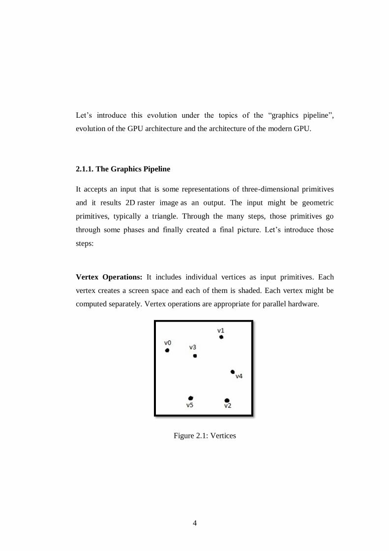
Vertex Operations: It includes individual vertices as input primitives. Each

vertex creates a screen space and each of them is shaded. Each vertex might be

computed separately. Vertex operations are appropriate for parallel hardware.

Figure 2.1: Vertices

5

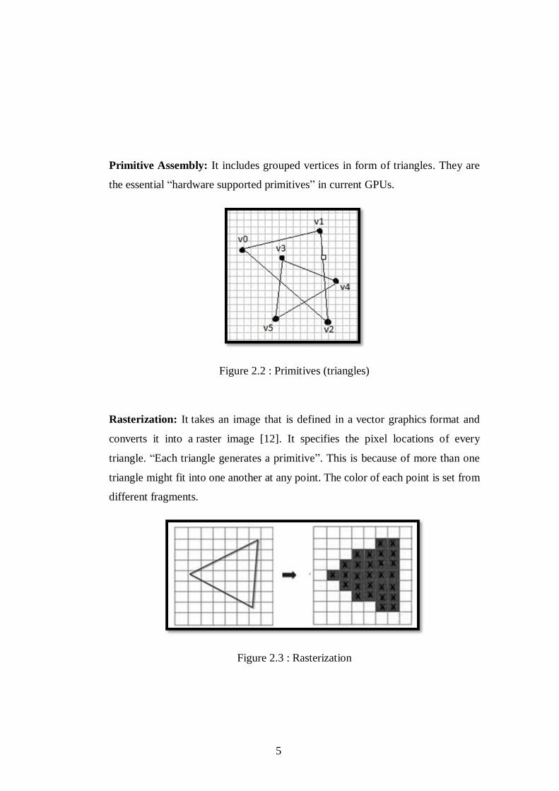
Primitive Assembly: It includes grouped vertices in form of triangles. They are

the essential “hardware supported primitives” in current GPUs.

Figure 2.2 : Primitives (triangles)

Rasterization: It takes an image that is defined in a vector graphics format and

converts it into a raster image [12]. It specifies the pixel locations of every

triangle. “Each triangle generates a primitive”. This is because of more than one

triangle might fit into one another at any point. The color of each point is set from

different fragments.

Figure 2.3 : Rasterization

6

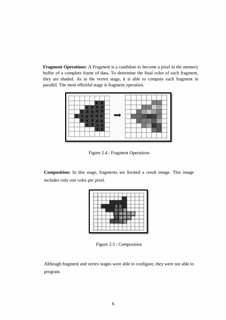
Fragment Operations: A Fragment is a candidate to become a pixel in the memory

buffer of a complete frame of data. To determine the final color of each fragment,

they are shaded. As in the vertex stage, it is able to compute each fragment in

parallel. The most effortful stage is fragment operation.

Figure 2.4 : Fragment Operations

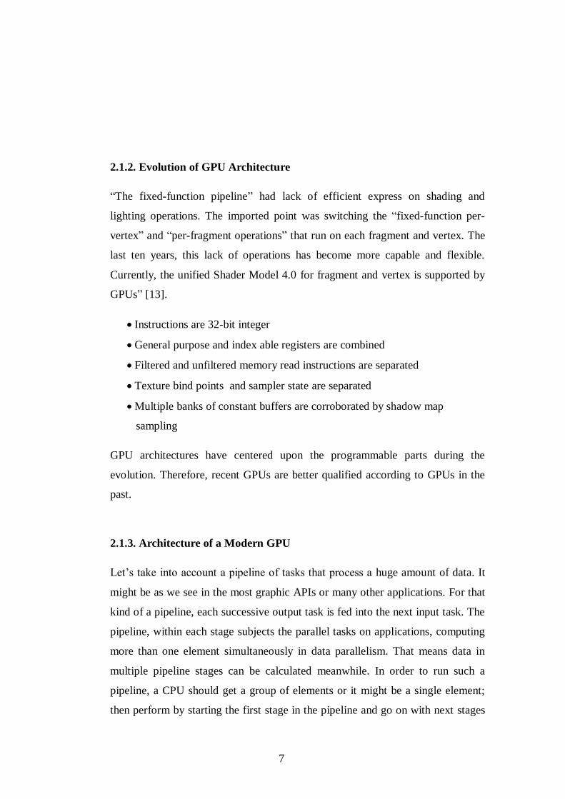
Composition: In this stage, fragments are formed a result image. This image

includes only one color per pixel.

Figure 2.5 : Composition

Although fragment and vertex stages were able to configure, they were not able to

program.

7

2.1.2. Evolution of GPU Architecture

“The fixed-function pipeline” had lack of efficient express on shading and

lighting operations. The imported point was switching the “fixed-function per-

vertex” and “per-fragment operations” that run on each fragment and vertex. The

last ten years, this lack of operations has become more capable and flexible.

Currently, the unified Shader Model 4.0 for fragment and vertex is supported by

GPUs” [13].

Instructions are 32-bit integer

General purpose and index able registers are combined

Filtered and unfiltered memory read instructions are separated

Texture bind points and sampler state are separated

Multiple banks of constant buffers are corroborated by shadow map

sampling

GPU architectures have centered upon the programmable parts during the

evolution. Therefore, recent GPUs are better qualified according to GPUs in the

past.

2.1.3. Architecture of a Modern GPU

Let‟s take into account a pipeline of tasks that process a huge amount of data. It

might be as we see in the most graphic APIs or many other applications. For that

kind of a pipeline, each successive output task is fed into the next input task. The

pipeline, within each stage subjects the parallel tasks on applications, computing

more than one element simultaneously in data parallelism. That means data in

multiple pipeline stages can be calculated meanwhile. In order to run such a

pipeline, a CPU should get a group of elements or it might be a single element;

then perform by starting the first stage in the pipeline and go on with next stages

8

and so on. The CPU splits the pipeline over time and applies all sources in the

processor to every stage respectively.

GPUs have a dissimilar approach according to CPU. A GPU separates the

processor resources between the different stages. The stage, the processor running

on, feeds the output into a different part which runs on the next stage.

That is pretty accomplished in “fixed-function GPUs”. It has two reasons on this

success. In the first place, for any given stage, the hardware makes use of data

parallelism at related stage. It processes multiple of elements at one and

simultaneously. This is because of most of the task-parallel stages were running

simultaneously and the GPU was able to reach the high compute requirements of

the graphics pipeline. Second reason is that; for a given task, every stage of

hardware would be customized. Special-purpose hardware is used for this. The

result of that, it allows greater compute and efficient area for general-purpose

solutions. If we think of rasterization stage, it is more effective if it is

implemented by using “special-purpose hardware”. When we think of vertex and

fragment programs, “the special purpose fixed function components” could be

easily replaced by programmable components. However, it does not mean task-

parallel organization is changed.

The final result was an improved GPU pipeline on many stages. Each of them is

expedited by using special purpose parallel hardware. While any operation might

get 20 cycles during CPU pipeline process, it might get thousands of cycles

during GPU pipeline process. The delay of any of the given operation is long, but,

the parallelism of data and tasks between stages has high throughput.

9

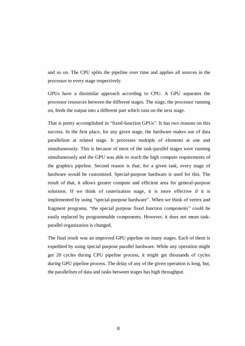
Figure 2.6 : Architecture of a modern NVIDIA graphics card

On task-parallel pipeline, the load balancing is the main disadvantage of the

GPU. The slowest stage determines the GPU performance. It depends on slowest

stage like any pipeline. If it has a complex vertex problem and a simple fragment

program, overall throughput will depend on slowest one – the vertex program.

We can say that the first generation of commodity data-parallel processors is

Modern GPUs. The highlighted advantages of those data-parallel computing are

extreme computational capacity and rapid growth curve. The most imported one

is they outstripped traditional CPUs. So, we can expect some generality and

enhanced programmability for the future GPU architectures [14].

10

Chapter 3

Overview of OpenCL

In all computing domains, heterogeneous parallel computing platforms are

extending their user base. Those platforms are consisted of varied processors such

as CPUs, GPUs, FPGAs, and DSPs. Beside the point of hi-performance with

admissible programming effort, parallel programming models should offer

portability between different processors.

“OpenCL (Open Computing Language) is a parallel programming model for such

heterogeneous platforms” [1], [2]. It is an open standard for programming

heterogeneous multiprocessor platforms. It allows the programmer to prepare

his/her application by setting up its computation as kernels. At all levels of

parallelism, you are free to parallelize the execution of kernel instances by using

OpenCL compiler. The applications on OpenCL are able to run on any

processors. They are even able to run between mixed processors.

According to traditional C programming language, OpenCL provides advanced

usage of parallelism in hardware constructs. And it is also familiar for the

programmers who have knowledge of C programming language [3].

“The goal of OpenCL is to become a preferred language for programming

platforms with heterogeneous processing devices such as CPUs, GPUs, FPGAs,

and DSPs”. The reason that OpenCL is a challenging candidate is that it provides

understandable description of parallel execution on lots of levels. It initializes

data level parallelism within a single kernel sample for its vector data types. “The

host API allows expressing the number of instances of kernels executed in

parallel for the number of work-groups". It also defines the execution platform

and the compiler as conveniently as possible.

11

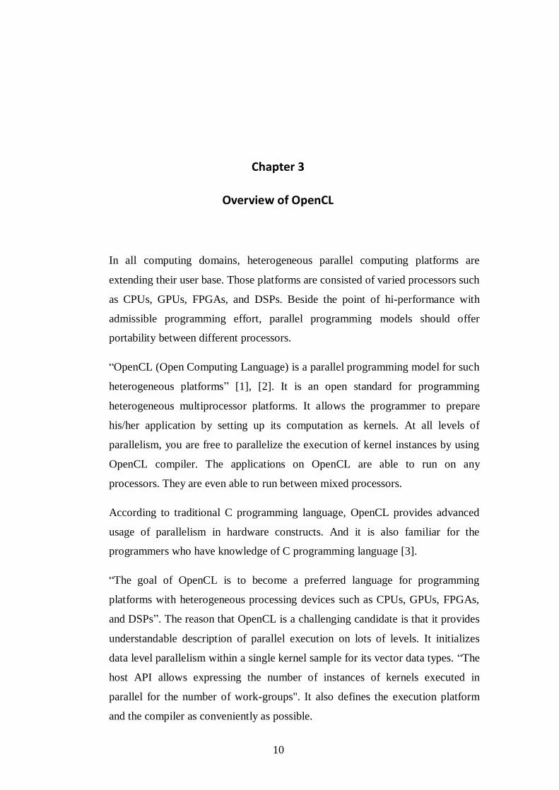
3.1. OpenCL Architecture

OpenCL is more than a programming language. “It is a framework for parallel

programming”. It also contains “API, libraries and a runtime system” in order to

corroborate software development. In this section, let‟s introduce the standard

OpenCL architecture [15] for GP GPUs and GPUs.

Figure 3.1 : OpenCL Architecture

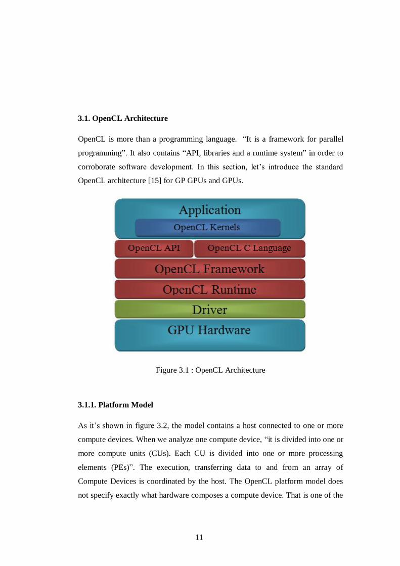
3.1.1. Platform Model

As it‟s shown in figure 3.2, the model contains a host connected to one or more

compute devices. When we analyze one compute device, “it is divided into one or

more compute units (CUs). Each CU is divided into one or more processing

elements (PEs)”. The execution, transferring data to and from an array of

Compute Devices is coordinated by the host. The OpenCL platform model does

not specify exactly what hardware composes a compute device. That is one of the

12

significant strengths of this model. By this way, a compute device may be a CPU

or a GPU or other processors.

Figure 3.2 : OpenCL Platform Model

13

3.1.2. Execution Model

An OpenCL execution is composed of two sections: a host program and kernels.

A host program identifies the context for kernels and directs kernels execution,

and runs on the host. Kernels execute on one compute device or more than one.

The most importing part of execution model is the kernels execution. When the

host submits a kernel, an index space is described. The index space that executes

a kernel is called NDRange. It is an N-dimensional space that includes an N-tuple

of integers, dimensions and size of the index space. Every point in this is

executed by the kernel instance. We called the kernel instance as a work-item. It

obtains a global ID of the work-item. This global ID is defined by the index space

of the point. Every work-item runs the same code with different execution

pathway that varies per work-items. One or more than one work-items are

associated into work-groups. Those groups include index spaces that assigned to

a unique work-group ID. So, each work-item has a unique local ID within a

workgroup.

This execution model can be used at a great variety of programming models.

3.1.3. Memory Model

In a compute device, there are four memory regions. These are “global memory,

constant memory, local memory and private memory”.

Global memory region has access of read and write in all work-groups and

therefore in all work-items. Constant memory stays as a constant while kernel is

executing. Local memory region is local to a work-group. It is used to assign

variables that are portioned out by whole work-items in that work-group. There is

also a private memory region which is private to a work-item and it means it is

invisible by other work-items.

14

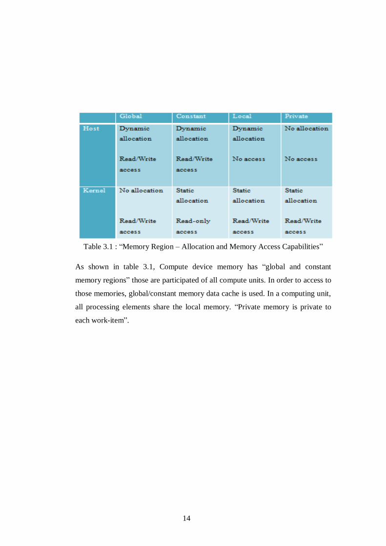
Table 3.1 : “Memory Region – Allocation and Memory Access Capabilities”

As shown in table 3.1, Compute device memory has “global and constant

memory regions” those are participated of all compute units. In order to access to

those memories, global/constant memory data cache is used. In a computing unit,

all processing elements share the local memory. “Private memory is private to

each work-item”.

15

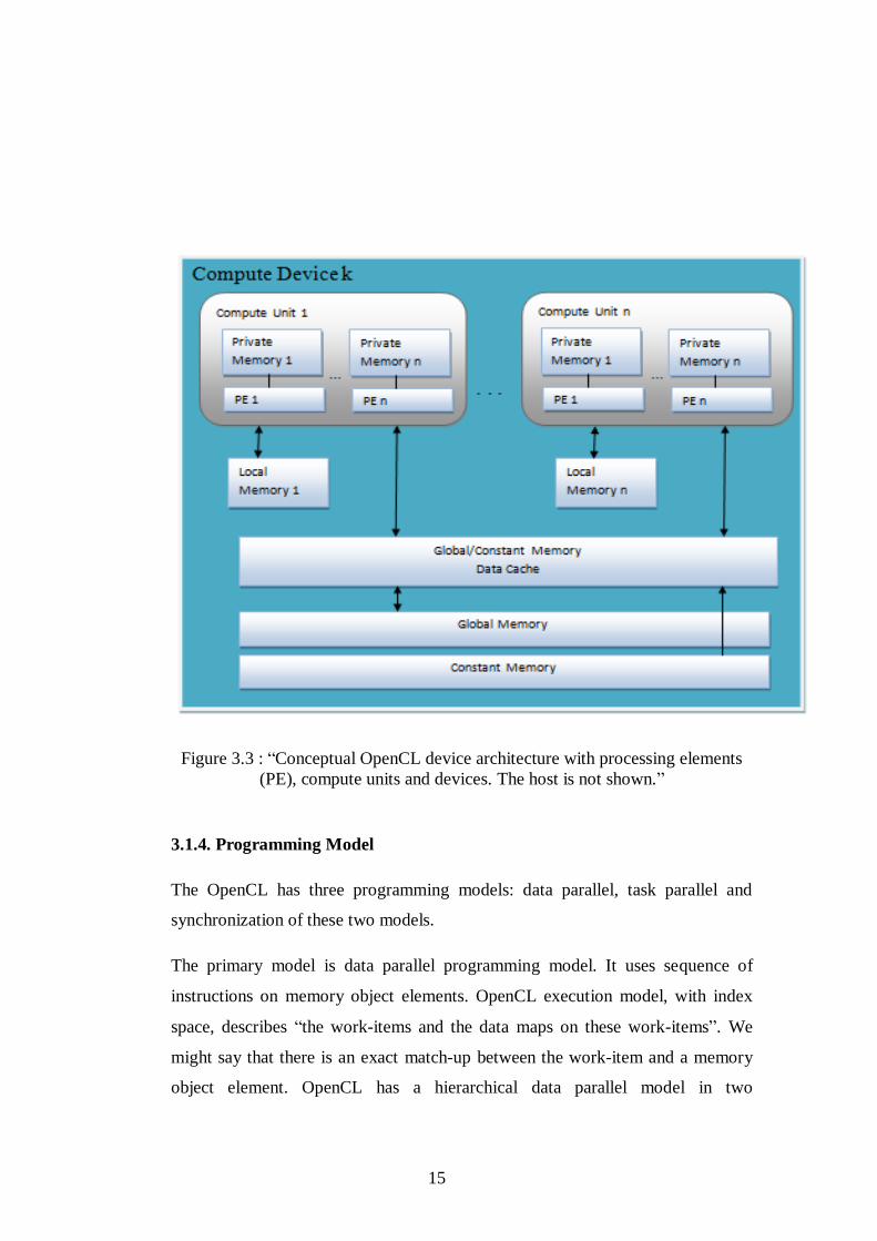
Figure 3.3 : “Conceptual OpenCL device architecture with processing elements

(PE), compute units and devices. The host is not shown.”

3.1.4. Programming Model

The OpenCL has three programming models: data parallel, task parallel and

synchronization of these two models.

The primary model is data parallel programming model. It uses sequence of

instructions on memory object elements. OpenCL execution model, with index

space, describes “the work-items and the data maps on these work-items”. We

might say that there is an exact match-up between the work-item and a memory

object element. OpenCL has a hierarchical data parallel model in two

16

ways: explicit model and implicit model. At explicit model, a programmer

identifies the number of work-items for parallelism and how work-items are

assigned among work-groups. At implicit model, a programmer defines only the

total number of work-items and assigning work-items among work-groups is

done by OpenCL implementation.

The second model is “task parallel programming model”. It uses a single kernel

instance that run for any index space independently. A kernel is executed on a CU

with a single work-item of a work-group. A programmer defines parallelism by

implementing vector data types on the device, enqueuing native kernels and/or

multiple tasks.

The last model is synchronization of data parallel model and task parallel model

in OpenCL. In this model, “work-items are in a single work-group and commands

are enqueued to command-queue(s) in a single context”. It uses work-group

barrier in order to provide concurrence of work-items of a work-group. Work-

groups does not include concurrence. The concurrence of commands are provided

by command-queue barrier and waiting on an event.

17

Chapter 4

Overview of OpenMP

OpenMP stands for Open Multi-Processing. “It is an API that is used to direct

multi-threaded, shared memory parallelism”. The API supports a wide range of

architectures on C/C++ and Fortran. It allows a portable and scalable model to for

developers.

OpenMP includes three primary components:

1. Directives and pragmas

2. Runtime library routines

3. Environment variables

Directive and pragmas include “control structures, work sharing, synchronization,

some data scope attributes and orphaning”. Runtime library routines include

“lock API, control and query routines like number of threads, nested parallelism”.

At environment variables, it has runtime environments such as schedule type,

maximum number of threads, throughput mode and nested parallelism.

OpenMP is being founded on shared memory programming for multiple threads.

It is a non-automatic programming model, because it offers the developer full

control over parallelization.

OpenMP uses the fork-joint model of parallel execution.

18

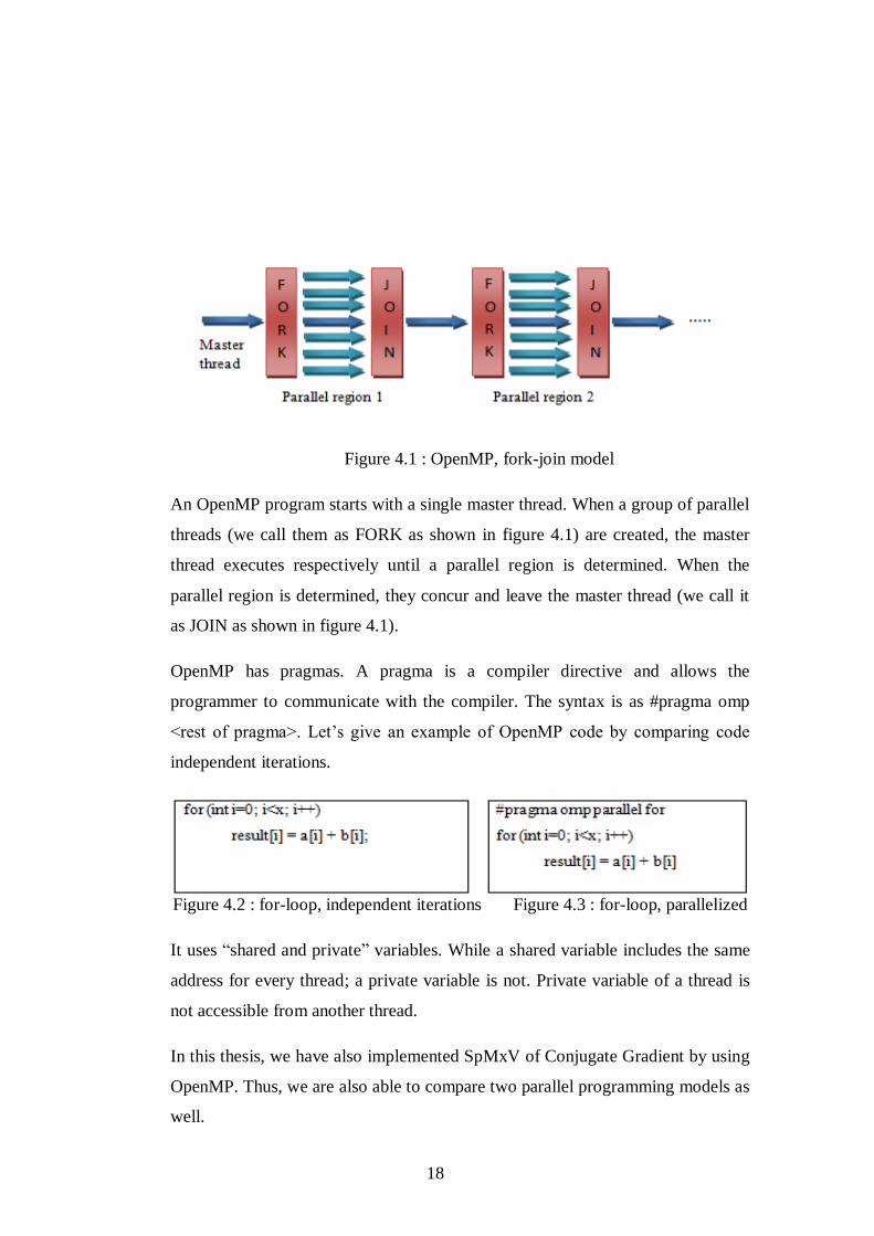
Figure 4.1 : OpenMP, fork-join model

An OpenMP program starts with a single master thread. When a group of parallel

threads (we call them as FORK as shown in figure 4.1) are created, the master

thread executes respectively until a parallel region is determined. When the

parallel region is determined, they concur and leave the master thread (we call it

as JOIN as shown in figure 4.1).

OpenMP has pragmas. A pragma is a compiler directive and allows the

programmer to communicate with the compiler. The syntax is as #pragma omp

<rest of pragma>. Let‟s give an example of OpenMP code by comparing code

independent iterations.

Figure 4.2 : for-loop, independent iterations Figure 4.3 : for-loop, parallelized

It uses “shared and private” variables. While a shared variable includes the same

address for every thread; a private variable is not. Private variable of a thread is

not accessible from another thread.

In this thesis, we have also implemented SpMxV of Conjugate Gradient by using

OpenMP. Thus, we are also able to compare two parallel programming models as

well.

19

Chapter 5

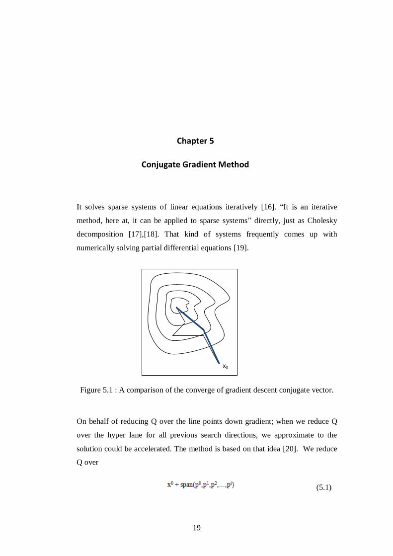
Conjugate Gradient Method

It solves sparse systems of linear equations iteratively [16]. “It is an iterative

method, here at, it can be applied to sparse systems” directly, just as Cholesky

decomposition [17],[18]. That kind of systems frequently comes up with

numerically solving partial differential equations [19].

Figure 5.1 : A comparison of the converge of gradient descent conjugate vector.

On behalf of reducing Q over the line points down gradient; when we reduce Q

over the hyper lane for all previous search directions, we approximate to the

solution could be accelerated. The method is based on that idea [20]. We reduce

Q over

(5.1)

x0

20

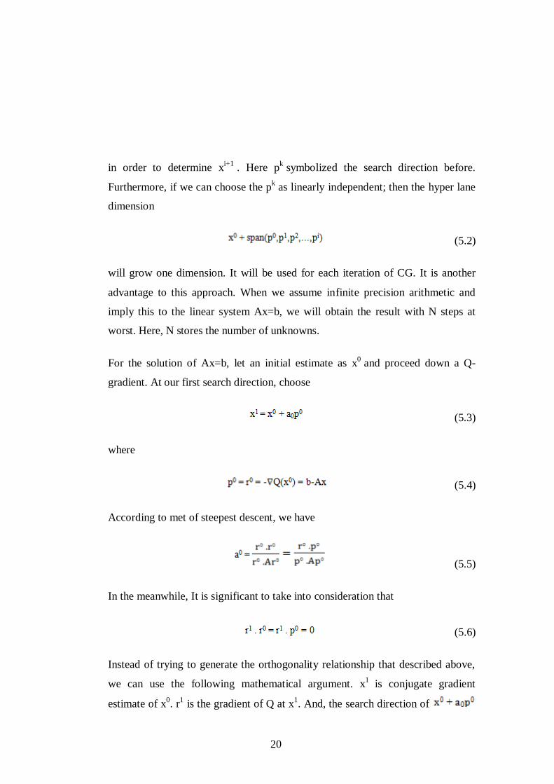
in order to determine xi+1

. Here pk symbolized the search direction before.

Furthermore, if we can choose the pk as linearly independent; then the hyper lane

dimension

(5.2)

will grow one dimension. It will be used for each iteration of CG. It is another

advantage to this approach. When we assume infinite precision arithmetic and

imply this to the linear system Ax=b, we will obtain the result with N steps at

worst. Here, N stores the number of unknowns.

For the solution of Ax=b, let an initial estimate as x0 and proceed down a Q-

gradient. At our first search direction, choose

(5.3)

where

(5.4)

According to met of steepest descent, we have

(5.5)

In the meanwhile, It is significant to take into consideration that

(5.6)

Instead of trying to generate the orthogonality relationship that described above,

we can use the following mathematical argument. x1

is conjugate gradient

estimate of x0. r

1 is the gradient of Q at x

1. And, the search direction of

21

is . The orthogonal to search direction at x1

is the gradient of Q according

to calculus.

In support of the statement above which is about calculus and orthogonality;

regard the onion layers with surfaces of Q is stable. And conjure up piercing it by

a skewer. The skewer will get through many layers of the onion as a rule. Then

touch one of the internal layers tangentially and get through other layers and

lastly exit. The internal layer inmost is given by Q(x1) = x

1 and r

0 = p

0 will be

the direction of the skewer.

Let‟s consider the skewered onion and the tending of r1 and r

0 = p

0.

The CG estimates by

(5.7)

(5.8)

By considering the equations above, we need to bear in mind two things while

selecting ai and βi . These are:

Fill the searching space as iterations increases number,

Search down Q-gradients. Use conjugate gradient search directions for this

purpose.

As we have learned what p0 and a

0, we can assume x

1 and r

1 = b - Ax

1 are known,

too. The following step to use the CG will be determining values for a0 and β1.

Then we will be able to calculate p1 and x

2.

At next step, we are searching to reduce Q over the plane:

(5.9)

22

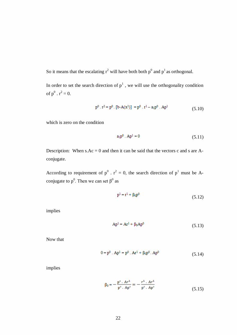
So it means that the escalating r2 will have both both p

0 and p

1 as orthogonal.

In order to set the search direction of p1 , we will use the orthogonality condition

of p0 . r

2 = 0.

(5.10)

which is zero on the condition

(5.11)

Description: When s.Ac = 0 and then it can be said that the vectors c and s are A-

conjugate.

According to requirement of p0 . r

2 = 0, the search direction of p

1 must be A-

conjugate to p0. Then we can set β

0 as

(5.12)

implies

(5.13)

Now that

(5.14)

implies

(5.15)

23

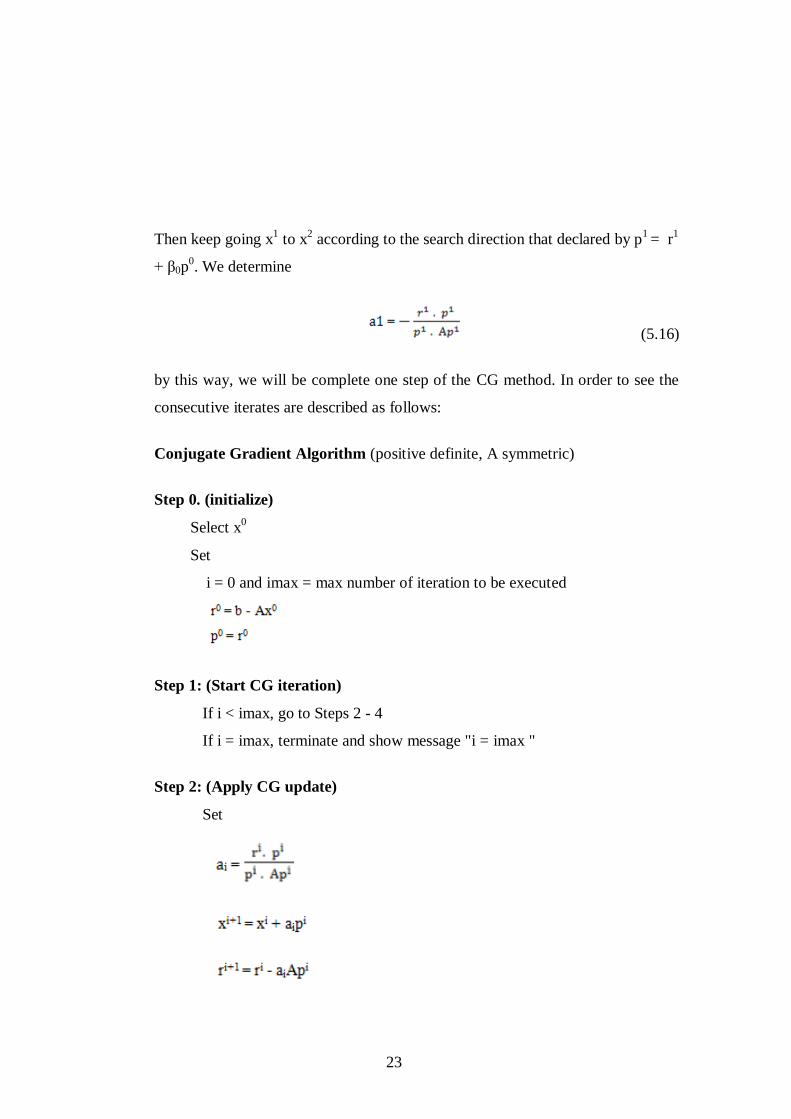
Then keep going x1 to x

2 according to the search direction that declared by p

1 = r

1

+ β0p0. We determine

(5.16)

by this way, we will be complete one step of the CG method. In order to see the

consecutive iterates are described as follows:

Conjugate Gradient Algorithm (positive definite, A symmetric)

Step 0. (initialize)

Select x0

Set

i = 0 and imax = max number of iteration to be executed

Step 1: (Start CG iteration)

If i < imax, go to Steps 2 - 4

If i = imax, terminate and show message "i = imax "

Step 2: (Apply CG update)

Set

24

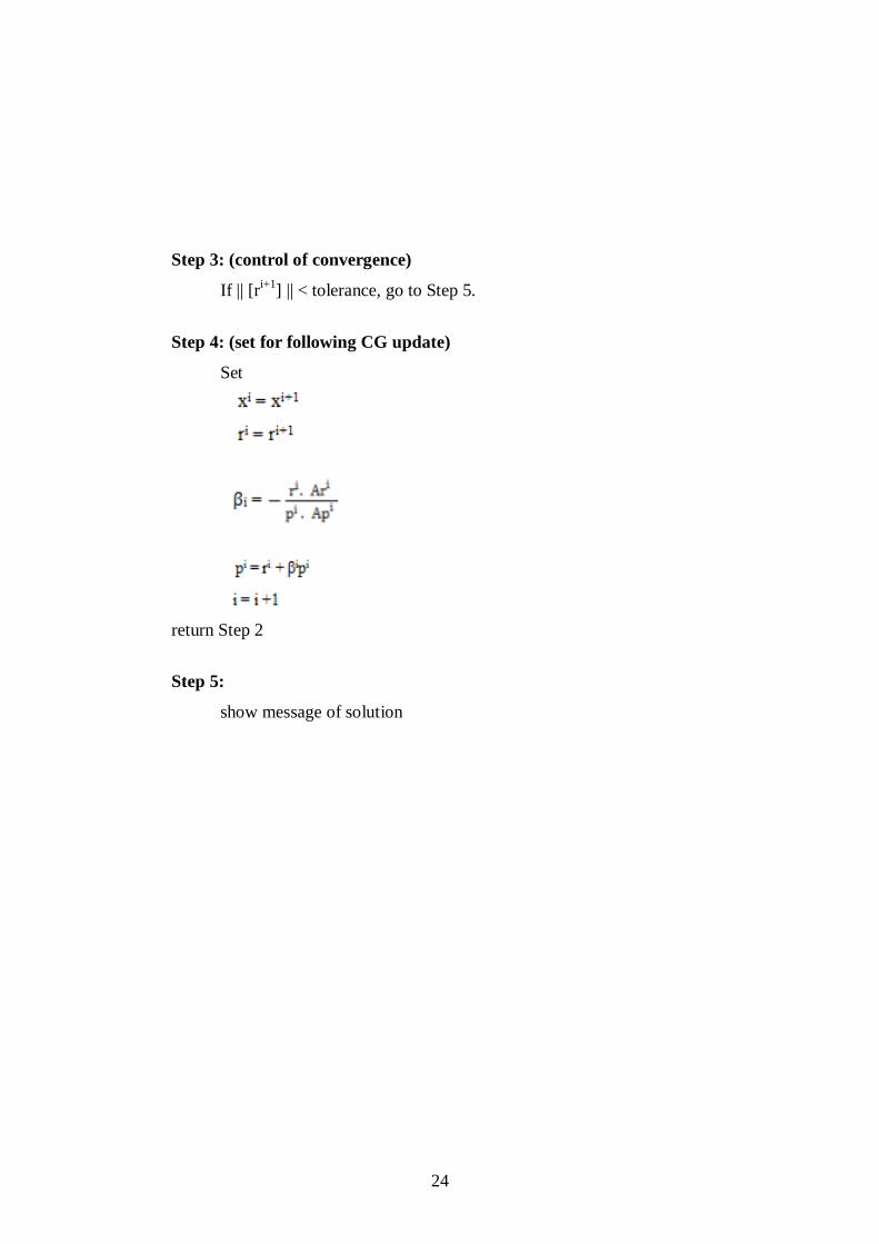
Step 3: (control of convergence)

If || [ri+1

] || < tolerance, go to Step 5.

Step 4: (set for following CG update)

Set

return Step 2

Step 5:

show message of solution

25

Chapter 6

Sparse Matrix Vector

Sparse matrix structures arise as a result of various computational disciplines.

The methods those manipulating them are typically related to the performance of

many applications. In computational science, sparse matrix-vector multiplication

(SpMV) operations have a certain importance. “They represent the dominant cost

in many iterative methods in order to solve large-scale linear systems.” [4]

We can define a sparse matrix as a matrix populated with zeros initially. The

recognized data structure for a matrix is a two-dimensional array. Each element

can be accesses by using indices i and j of represented element aij. Enough

memory storage for an m×n matrix is shown as (m×n) entries [21].

5.1. Compressed Sparse Row Format:

The sparse matrix storage includes various formats. They all have commonly

designed for SpMxV. “The compressed sparse rows (CSR) format has problems

on low performance for the indirect addressing. The reading the elements of

sparse matrix has a strong impact on the performance”. As a result of this, each

specific algorithm that computes SpMxV uses a specific architecture of these

specific storage formats [22]. There are several studies published about this

problem of SpMxV [23], [24], [25].

There are many matrix storage choices such as COO, CSR, CSC, DIAG, ELL and

HYB (ELL+CSR). During our study, we will focus on the compress sparse

matrix (CSR).

26

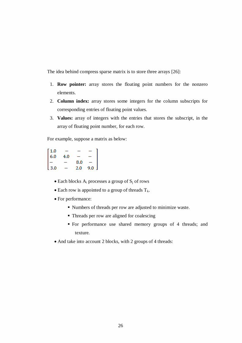
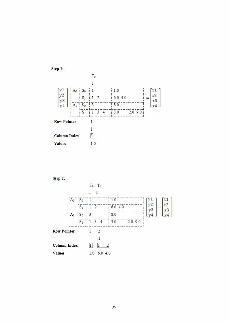
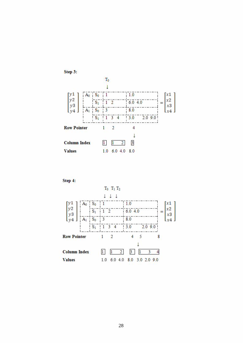
The idea behind compress sparse matrix is to store three arrays [26]:

1. Row pointer: array stores the floating point numbers for the nonzero

elements.

2. Column index: array stores some integers for the column subscripts for

corresponding entries of floating point values.

3. Values: array of integers with the entries that stores the subscript, in the

array of floating point number, for each row.

For example, suppose a matrix as below:

Each blocks Ai processes a group of Sj of rows

Each row is appointed to a group of threads Tk.

For performance:

Numbers of threads per row are adjusted to minimize waste.

Threads per row are aligned for coalescing

For performance use shared memory groups of 4 threads; and

texture.

And take into account 2 blocks, with 2 groups of 4 threads:

27

28

29

The result shows that there are 8 values those are 1.0, 6.0, 4.0, 8.0, 3.0, 2.0 and

9.0. Those values are defined with row pointers and grouped column indexes.

There are 4 rows and it is defined the nonzero columns with their index numbers.

The example above is solved as row based. It might be solved as column base

also.

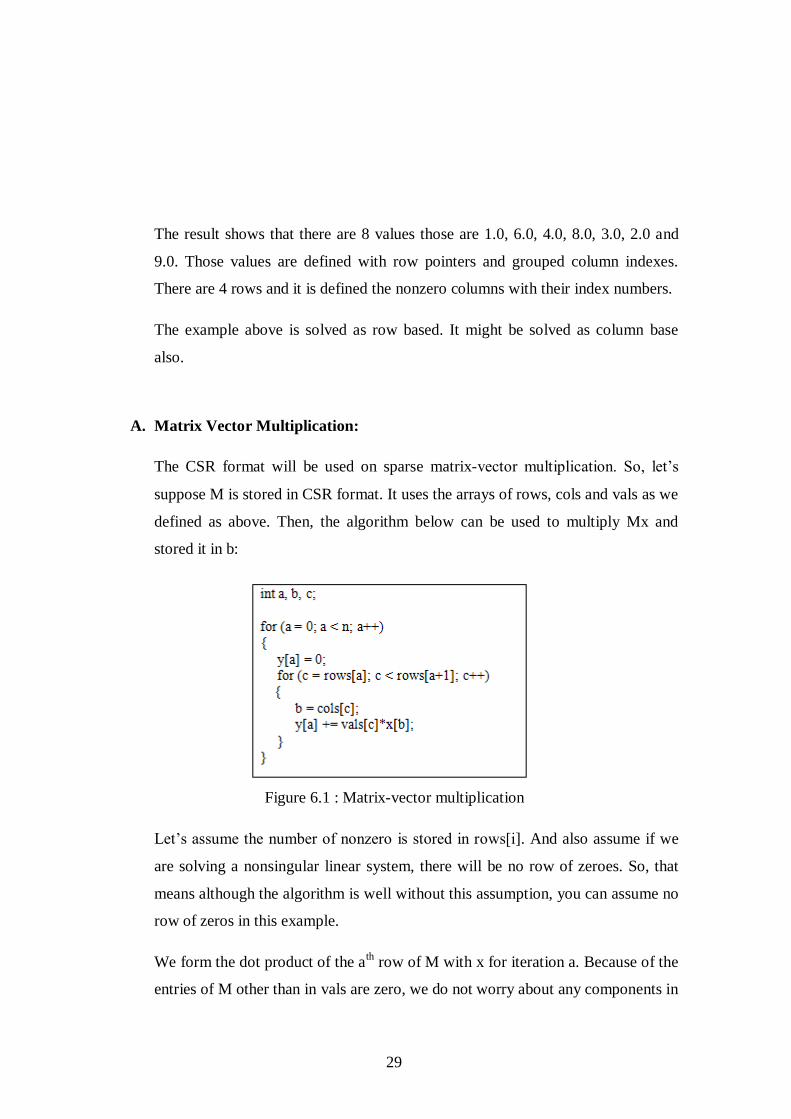
A. Matrix Vector Multiplication:

The CSR format will be used on sparse matrix-vector multiplication. So, let‟s

suppose M is stored in CSR format. It uses the arrays of rows, cols and vals as we

defined as above. Then, the algorithm below can be used to multiply Mx and

stored it in b:

Figure 6.1 : Matrix-vector multiplication

Let‟s assume the number of nonzero is stored in rows[i]. And also assume if we

are solving a nonsingular linear system, there will be no row of zeroes. So, that

means although the algorithm is well without this assumption, you can assume no

row of zeros in this example.

We form the dot product of the ath

row of M with x for iteration a. Because of the

entries of M other than in vals are zero, we do not worry about any components in

30

row a. Moreover, when the nonzero elements in the ath

row of M are stored

sequential entries of vals. Those run between row[a] and row [a+1]. We do the

calculation on the ath

row with corresponding x by multiplying these elements of

vals.

In this thesis, GPU code is parallelized for only sparse matrix vector. And

heterogeneous programming library (HPL) [5] is used for this purpose. HPL

allows a novel library-based approach to programming heterogeneous systems

and supports the user with portability with ease of use. It provides the usual C++

control flow structures such as „if‟, „for‟. There are three differences. The names

of control structures are finish with underscores like „if_‟. The end of blocks must

be closed with related statement with underscore like „endif_‟. The last difference

is for_ statement. It includes commas instead of semicolons.

31

Chapter 7

Performance

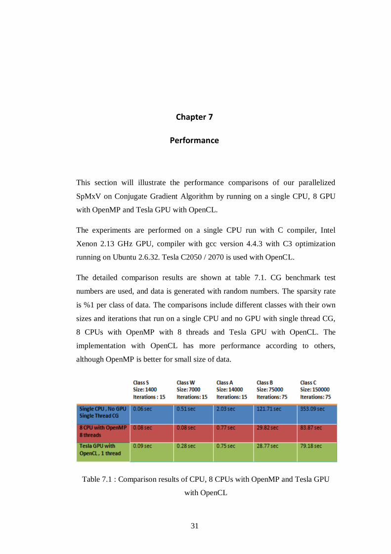
This section will illustrate the performance comparisons of our parallelized

SpMxV on Conjugate Gradient Algorithm by running on a single CPU, 8 GPU

with OpenMP and Tesla GPU with OpenCL.

The experiments are performed on a single CPU run with C compiler, Intel

Xenon 2.13 GHz GPU, compiler with gcc version 4.4.3 with C3 optimization

running on Ubuntu 2.6.32. Tesla C2050 / 2070 is used with OpenCL.

The detailed comparison results are shown at table 7.1. CG benchmark test

numbers are used, and data is generated with random numbers. The sparsity rate

is %1 per class of data. The comparisons include different classes with their own

sizes and iterations that run on a single CPU and no GPU with single thread CG,

8 CPUs with OpenMP with 8 threads and Tesla GPU with OpenCL. The

implementation with OpenCL has more performance according to others,

although OpenMP is better for small size of data.

Table 7.1 : Comparison results of CPU, 8 CPUs with OpenMP and Tesla GPU

with OpenCL

32

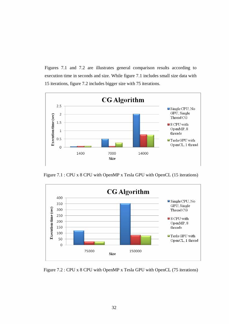
Figures 7.1 and 7.2 are illustrates general comparison results according to

execution time in seconds and size. While figure 7.1 includes small size data with

15 iterations, figure 7.2 includes bigger size with 75 iterations.

Figure 7.1 : CPU x 8 CPU with OpenMP x Tesla GPU with OpenCL (15 iterations)

Figure 7.2 : CPU x 8 CPU with OpenMP x Tesla GPU with OpenCL (75 iterations)

33

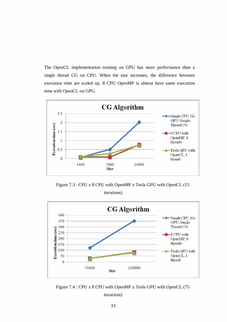
The OpenCL implementation running on GPU has more performance than a

single thread CG on CPU. When the size increases, the difference between

execution time are scaled up. 8 CPU OpenMP is almost have same execution

time with OpenCL on GPU.

Figure 7.3 : CPU x 8 CPU with OpenMP x Tesla GPU with OpenCL (15

iterations)

Figure 7.4 : CPU x 8 CPU with OpenMP x Tesla GPU with OpenCL (75

iterations)

34

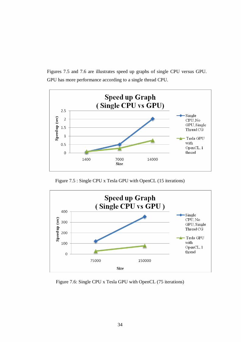
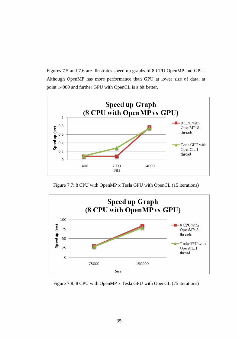
Figures 7.5 and 7.6 are illustrates speed up graphs of single CPU versus GPU.

GPU has more performance according to a single thread CPU.

Figure 7.5 : Single CPU x Tesla GPU with OpenCL (15 iterations)

Figure 7.6: Single CPU x Tesla GPU with OpenCL (75 iterations)

35

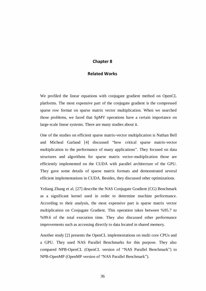
Figures 7.5 and 7.6 are illustrates speed up graphs of 8 CPU OpenMP and GPU.

Although OpenMP has more performance than GPU at lower size of data, at

point 14000 and further GPU with OpenCL is a bit better.

Figure 7.7: 8 CPU with OpenMP x Tesla GPU with OpenCL (15 iterations)

Figure 7.8: 8 CPU with OpenMP x Tesla GPU with OpenCL (75 iterations)

36

Chapter 8

Related Works

We profiled the linear equations with conjugate gradient method on OpenCL

platforms. The most expensive part of the conjugate gradient is the compressed

sparse row format on sparse matrix vector multiplication. When we searched

those problems, we faced that SpMV operations have a certain importance on

large-scale linear systems. There are many studies about it.

One of the studies on efficient sparse matrix-vector multiplication is Nathan Bell

and Micheal Garland [4] discussed “how critical sparse matrix-vector

multiplication to the performance of many applications”. They focused on data

structures and algorithms for sparse matrix vector-multiplication those are

efficiently implemented on the CUDA with parallel architecture of the GPU.

They gave some details of sparse matrix formats and demonstrated several

efficient implementations in CUDA. Besides, they discussed other optimizations.

Yeliang Zhang et al. [27] describe the NAS Conjugate Gradient (CG) Benchmark

as a significant kernel used in order to determine machine performance.

According to their analysis, the most expensive part is sparse matrix vector

multiplication on Conjugate Gradient. This operation takes between %95.7 to

%99.6 of the total execution time. They also discussed other performance

improvements such as accessing directly to data located in shared memory.

Another study [2] presents the OpenCL implementations on multi core CPUs and

a GPU. They used NAS Parallel Benchmarks for this purpose. They also

compared NPB-OpenCL (OpenCL version of “NAS Parallel Benchmark”) to

NPB-OpenMP (OpenMP version of “NAS Parallel Benchmark”).

37

Nahid Emad et al [28] have study on sparse matrix-vector product optimization.

They focused on sparse matrix on CSR format. They studied on an optimization

technique and apply this to sparse matrix-vector product. They performed their

experiments on three different machines and compared the results.

“Accelerating sparse matrix vector multiplication in iterative methods using

GPU" is another study about this [29]. They considered sparse matrix with a

vector as a primary operation on linear algebra kernels. They chose an

appropriate data structure for it and improved the performance of the spmv

kernels. They also gain %20 improvement on their spmv in the conjugate

gradient.

P. Sadayappan et al [30] present improvements “the performance of sparse

matrix-vector multiplication”. They studied on “single-node” performance of

spmv on compressed-sparse row format. During their studies, they focused on

“data locality” and “fine-grained parallelism”.

There is another study on “understanding the performance of sparse matrix-vector

multiplication” [31]. In this study, the performance issues used spmv kernel on

modern micro architectures is discussed. In order to understand SpMxV

performance better, they performed some experiments on different hardware

platforms. As a result, they represent useful results about this.

38

Chapter 9

Conclusion

In this thesis, we have researched the structures of GPU, OpenCL platform,

Conjugate Gradient Method and Sparse Matrix Vector on CSR format. We have

given examples in real life and many figures to facilitate to understand. Besides

the offered method, we have also compared the results on different platforms.

During the thesis, the most costly part of Conjugate gradient method – sparse

matrix-vector multiplication is discussed. It is proposed to use CSR format for

sparse matrix-vector multiplication on OpenCL platform. The GPU

parallelization is provided by using HPL (heterogeneous programming library).

We have provided 3 different implementation codes of conjugate gradient. These

are running on a single CPU without GPU and with a single thread CG, running

on 8 CPUs with OpenMP (includes 8 threads) and the proposed implementation

running on Tesla GPU with OpenCL and parallelization of GPU with HPL.

We evaluated the performance and scalability of proposed method by comparing

the others. While proposed implementation provides huge amount of performance

according to a single CPU, it has an increasing performance on OpenMP in direct

proportion to data size.

39

References

[1] “OpenCL Specification v1.0r48”, Khronos Group, Oct. 2009, [Online],

Available: http://www.khronos.org/registry/cl/

[2] Sangmin Seo, Gangwon Jo, Jaejin Lee, “Performance Characterization of the

NAS Parallel Benchmarks in OpenCL”, pp. 137-148, Seoul National University,

Seoul, 2011

[3] Pekka O. Jaaskelainen, Carlos S. de La Lama , Pablo Huerta and Jarmo H.

Takala , “OpenCL-based Design Methodology for Application-Specific

Processors”, pp. 223-230, IEEE, 2010

[4] Nathan Bell, Michael Garland, “Efficient Sparse Matrix-Vector Multiplication

on CUDA”, December 2008

[5] Zeki Bozkuş and Basilio B. Fraguela, “A portable high-Productivity

Approach to Program Heterogeneous Systems”, 2012

[6] https://computing.llnl.gov/tutorials/openMP/

[7] http://developers.sun.com/solaris/articles/openmp.html

[8] Ayguade, E.; Copty, N. ; Duran, A. ; Hoeflinger, J. ; Yuan Lin ; Massaioli,

F.; Teruel, X. ; Unnikrishnan, P. and Guansong Zhang , “The Design of

OpenMP Tasks”, Vol. 20, pp. 404 – 418, March 2009

[9] John D. Owens, Mike Houston, David Luebke, Simon Green, John E. Stone,

and James C. Phillips, “GPU Computing”, Vol. 96, No. 5, pp. 879-899, May

2008

[10] http://en.wikipedia.org/wiki/Graphics_processing_unit

[11] http://www.sharpened.net/glossary/definition/gpu

40

[12] http://en.wikipedia.org/wiki/Rasterisation

[13] D. Blythe, “BThe Direct3D 10 system”, ACM Trans. Graph., vol. 25, no. 3,

pp. 724–734, Aug. 2006.

[14] Luebke and Greg Humphreys, “How GPUs work”, IEEE Computer, Vol. 40

No. 2, pp 126-130, February 2007.

[15] Khronos OpenCL Working Group, “The OpenCL specification version 1.0”,

http://www.khronos.org/opencl.

[16] Audun Torp, “Sparse linear algebra on a GPU with Applications to flow in

porous Media”, Jan 2009

[17] Magnus R.Hestenes, Eduard Stiefel, “Methods of Conjugate Gradients for

Solving Linear Systems”, Research paper 2379, Vol. 49, No.6, pp. 409-436,

December 1952

[18] http://en.wikipedia.org/wiki/Cholesky_decomposition

[19] http://en.wikipedia.org/wiki/Conjugate_gradient_method

[20]http://cauchy.math.colostate.edu/Resources/SD_CG/conjgrad/node1.html

[21] http://en.wikipedia.org/wiki/Sparse_matrix

[22] F. V´azquez, G. Ortega, J.J. Fern´andez, E.M. Garz´on, “Improving the

performance of the sparse matrix vector product with GPUs”, 10th IEEE

International Conference on Computer and Information Technology, 2010

[23] Pavel Tvrdik, Ivan Simecek, “A New Approach for Accelerating the Sparse

Matrix-vector Multiplication”, IEEE , 2006

[24] E. Im. , “Optimizing the Performance of Sparse Matrix-Vector

Multiplication - dissertation thesis”, University of Carolina at Berkeley, 2001

41

[25] J. Mellor-Crummey and J. Garvin, “Optimizing sparse matrix vector product

computations using unroll and jam”, International Journal of High Performance

Computing Applications, 18(2):225–236, 2004

[26] M. Naumov, L. S. Chien, P. Vandermersch and U. Kapasi, “CUSPARSE

Library”, GPU Technology Conference, NVIDIA, September 2010

[27] Yelin Zhang, Vinod Tipparaju, Jarek Nieplocha, Salim Hariri,

“Parallelization of the NAS Conjugate Gradient Benchmark Using the Global

Arrays Shared Memory Programming Model”, Workshop 4 - Volume 05,

IPDPS'05, 2005

[28] Nahid EMAD, Olfa HAMDI-LARBI, Zaher MAHJOUB, “On Sparse

Matrix-Vector Optimization”, IEEE 2005

[29] Kiran Kumar Matam, Kishore Kothapalli, “Accelerating Sparse Matrix

Vector Multiplication in Iterative Methos Using GPU”, IEEE 2011

[30] James b. White, P. Sadayappan, “On Improving the Performance of Sparse

Matrix-Vector Multiplication”, IEEE 1997

[31] Goumas, Kornilios Kourtis, Nikos Anastopoulos, Vasileios Karakasis and

Nectarios Koziris, “Understanding the Performance of Sparse Matrix-Vector

Multiplication”, IEEE 2008

42

Curriculum Vitae

Caner Sayin was born on 20 August 1985, in Istanbul. He received his BS degree

in Computer Engineering in 2009 from Kadir Has University. He worked as a

research assistant at the department of Computer Engineering of Kadir Has

University from 2009 – 2010. Then he has been working as a SQL Developer at

KLM Royal Dutch Airlines since 2010. During his master education, he has been

affiliated with the Parallel Programming. His research interests include data

mining, relational databases and java technologies.

APPENDIX B APPENDIX B