Embed Size (px)
Citation preview
L. Vandenberghe EE236C (Spring 2016)
3. Conjugate gradient method
• conjugate gradient method for linear equations
• convergence analysis
• conjugate gradient method as iterative method
• applications in nonlinear optimization
3-1
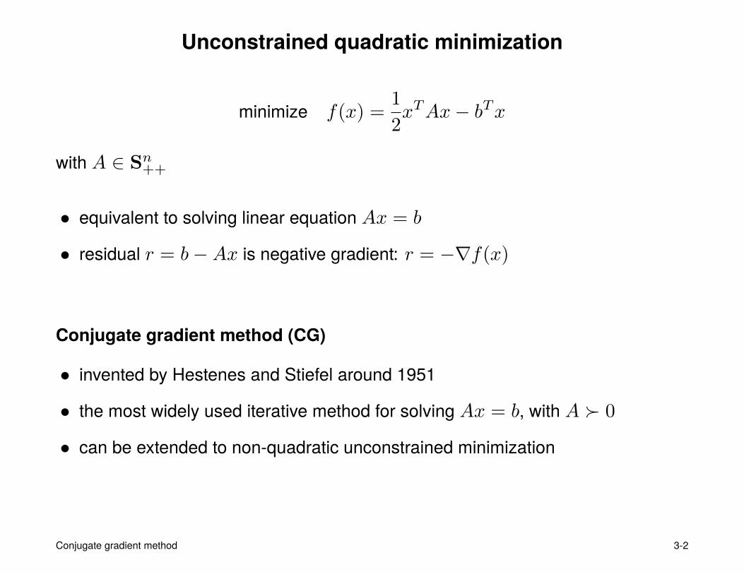
Unconstrained quadratic minimization
minimize f(x) =1
2xTAx− bTx
with A ∈ Sn++
• equivalent to solving linear equation Ax = b
• residual r = b−Ax is negative gradient: r = −∇f(x)
Conjugate gradient method (CG)
• invented by Hestenes and Stiefel around 1951
• the most widely used iterative method for solving Ax = b, with A � 0
• can be extended to non-quadratic unconstrained minimization
Conjugate gradient method 3-2
Krylov subspaces
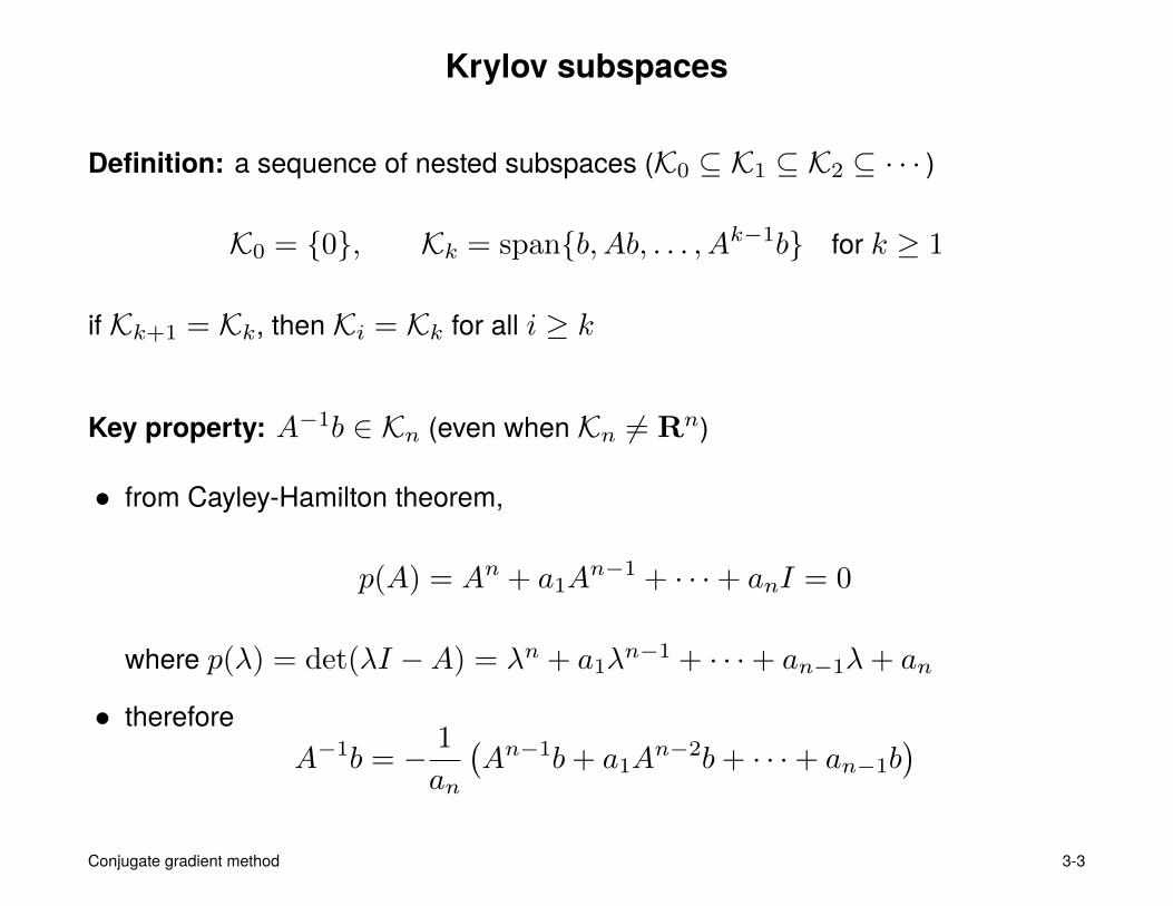
Definition: a sequence of nested subspaces (K0 ⊆ K1 ⊆ K2 ⊆ · · · )
K0 = {0}, Kk = span{b, Ab, . . . , Ak−1b} for k ≥ 1
if Kk+1 = Kk, then Ki = Kk for all i ≥ k
Key property: A−1b ∈ Kn (even when Kn 6= Rn)
• from Cayley-Hamilton theorem,
p(A) = An + a1An−1 + · · ·+ anI = 0
where p(λ) = det(λI −A) = λn + a1λn−1 + · · ·+ an−1λ+ an
• thereforeA−1b = − 1
an
(An−1b+ a1A
n−2b+ · · ·+ an−1b)
Conjugate gradient method 3-3
Krylov sequence
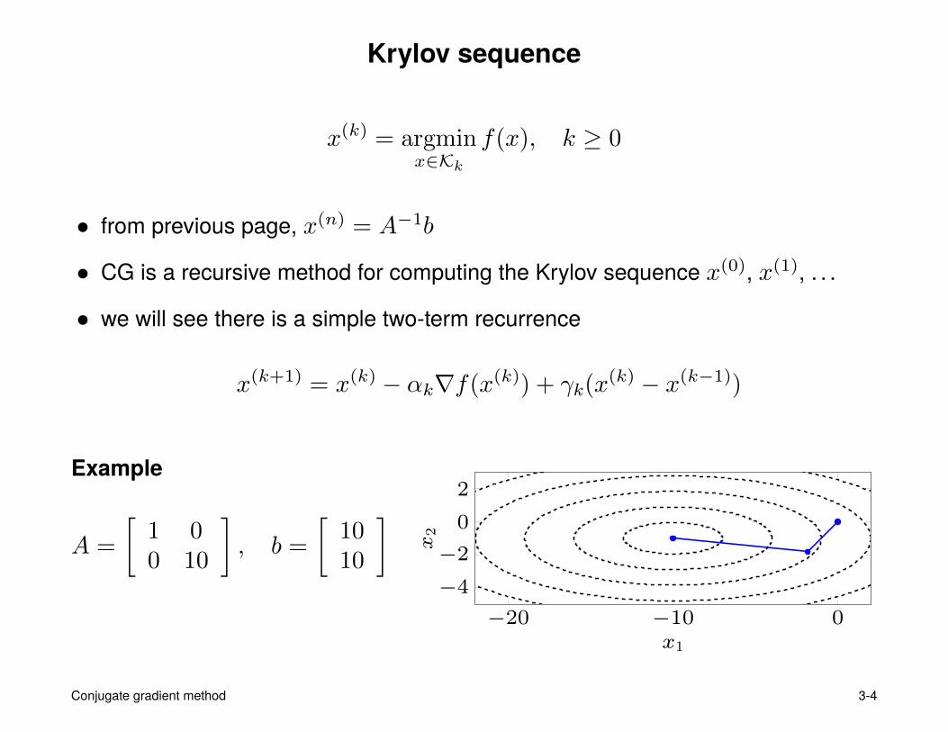
x(k) = argminx∈Kk
f(x), k ≥ 0
• from previous page, x(n) = A−1b
• CG is a recursive method for computing the Krylov sequence x(0), x(1), . . .
• we will see there is a simple two-term recurrence
x(k+1) = x(k) − αk∇f(x(k)) + γk(x(k) − x(k−1))
Example
A =
[1 00 10
], b =
[1010
]−20 −10 0
−4
−2
0
2
x1
x2
Conjugate gradient method 3-4
Residuals of Krylov sequence
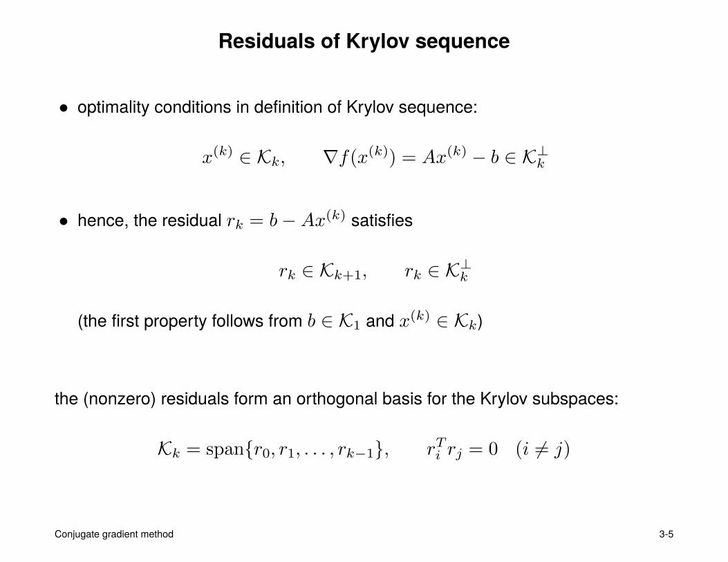
• optimality conditions in definition of Krylov sequence:
x(k) ∈ Kk, ∇f(x(k)) = Ax(k) − b ∈ K⊥k
• hence, the residual rk = b−Ax(k) satisfies
rk ∈ Kk+1, rk ∈ K⊥k
(the first property follows from b ∈ K1 and x(k) ∈ Kk)
the (nonzero) residuals form an orthogonal basis for the Krylov subspaces:
Kk = span{r0, r1, . . . , rk−1}, rTi rj = 0 (i 6= j)
Conjugate gradient method 3-5
Conjugate directions
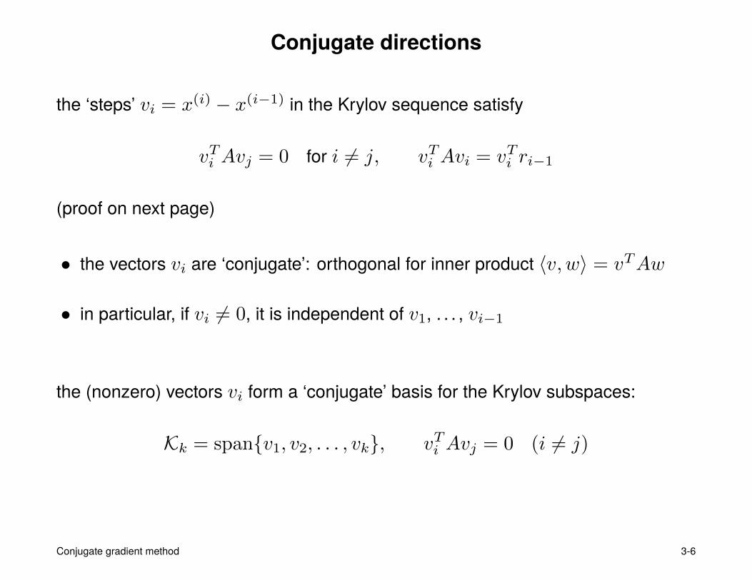
the ‘steps’ vi = x(i) − x(i−1) in the Krylov sequence satisfy
vTi Avj = 0 for i 6= j, vTi Avi = vTi ri−1
(proof on next page)
• the vectors vi are ‘conjugate’: orthogonal for inner product 〈v, w〉 = vTAw
• in particular, if vi 6= 0, it is independent of v1, . . . , vi−1
the (nonzero) vectors vi form a ‘conjugate’ basis for the Krylov subspaces:
Kk = span{v1, v2, . . . , vk}, vTi Avj = 0 (i 6= j)
Conjugate gradient method 3-6
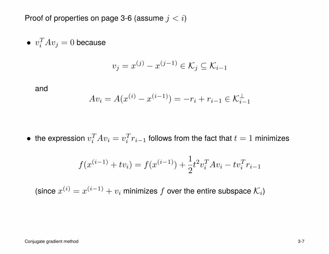
Proof of properties on page 3-6 (assume j < i)
• vTi Avj = 0 because
vj = x(j) − x(j−1) ∈ Kj ⊆ Ki−1
andAvi = A(x(i) − x(i−1)) = −ri + ri−1 ∈ K⊥i−1
• the expression vTi Avi = vTi ri−1 follows from the fact that t = 1 minimizes
f(x(i−1) + tvi) = f(x(i−1)) +1
2t2vTi Avi − tvTi ri−1
(since x(i) = x(i−1) + vi minimizes f over the entire subspace Ki)
Conjugate gradient method 3-7
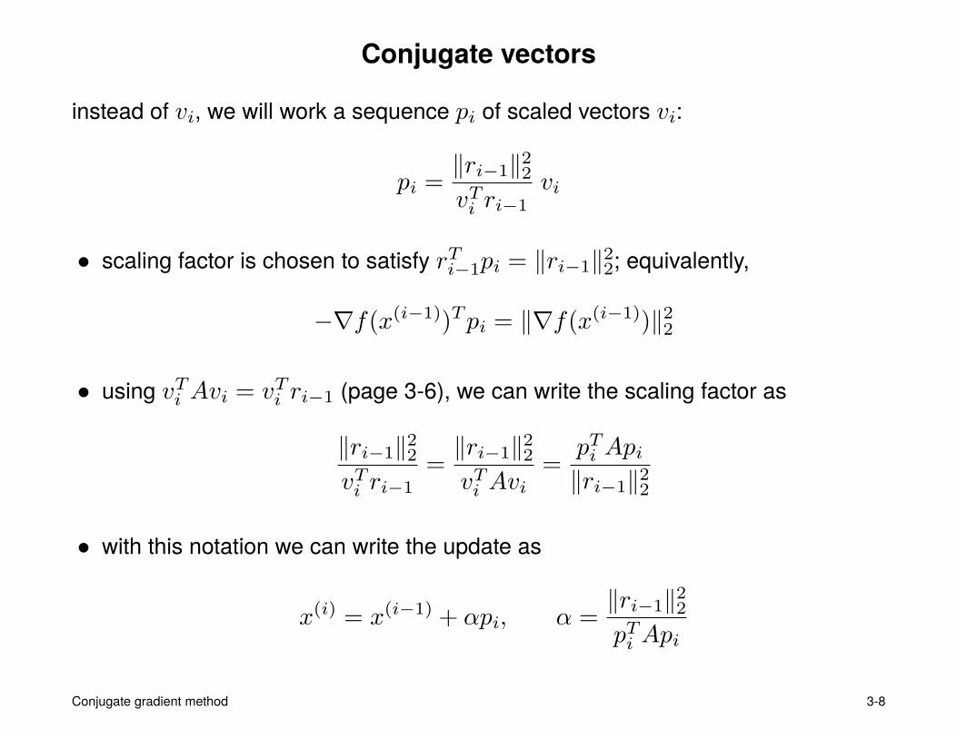
Conjugate vectors
instead of vi, we will work a sequence pi of scaled vectors vi:
pi =‖ri−1‖22vTi ri−1
vi
• scaling factor is chosen to satisfy rTi−1pi = ‖ri−1‖22; equivalently,
−∇f(x(i−1))Tpi = ‖∇f(x(i−1))‖22
• using vTi Avi = vTi ri−1 (page 3-6), we can write the scaling factor as
‖ri−1‖22vTi ri−1
=‖ri−1‖22vTi Avi
=pTi Api‖ri−1‖22
• with this notation we can write the update as
x(i) = x(i−1) + αpi, α =‖ri−1‖22pTi Api
Conjugate gradient method 3-8
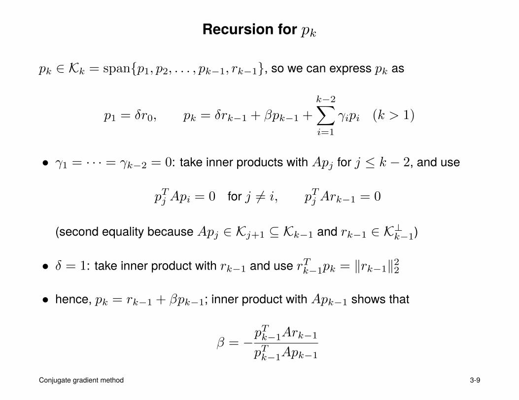
Recursion for pk
pk ∈ Kk = span{p1, p2, . . . , pk−1, rk−1}, so we can express pk as
p1 = δr0, pk = δrk−1 + βpk−1 +
k−2∑i=1
γipi (k > 1)
• γ1 = · · · = γk−2 = 0: take inner products with Apj for j ≤ k − 2, and use
pTj Api = 0 for j 6= i, pTj Ark−1 = 0
(second equality because Apj ∈ Kj+1 ⊆ Kk−1 and rk−1 ∈ K⊥k−1)
• δ = 1: take inner product with rk−1 and use rTk−1pk = ‖rk−1‖22
• hence, pk = rk−1 + βpk−1; inner product with Apk−1 shows that
β = −pTk−1Ark−1
pTk−1Apk−1
Conjugate gradient method 3-9
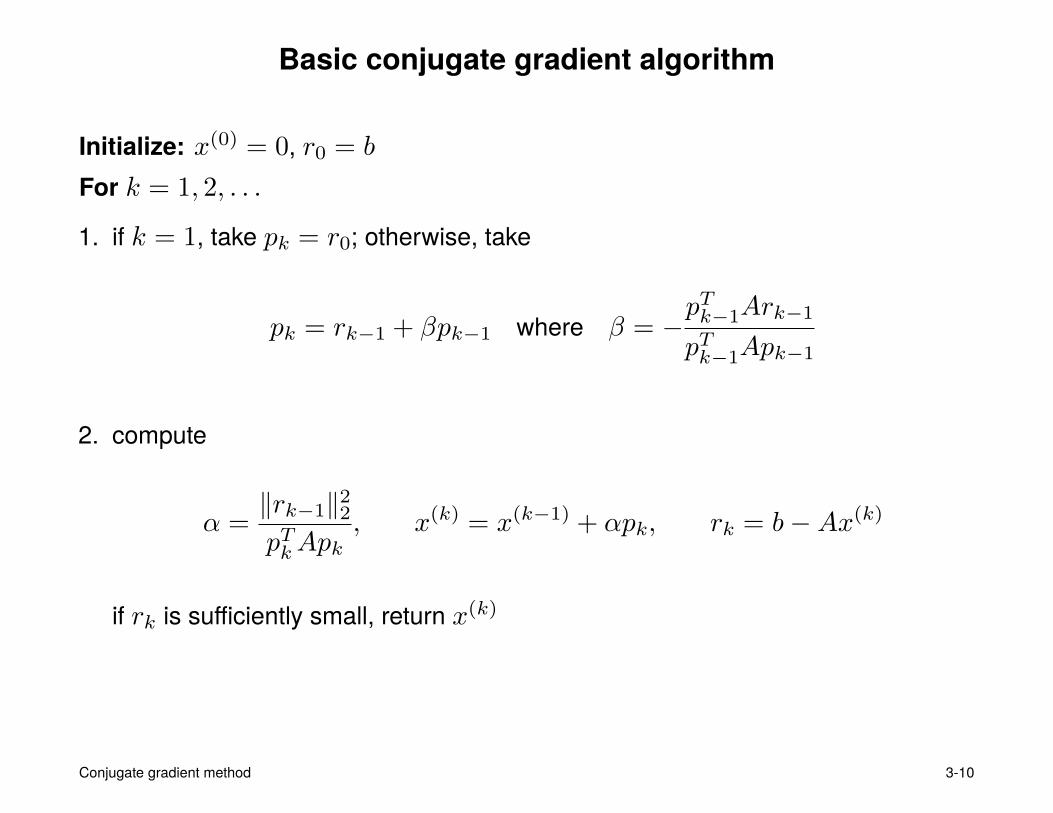
Basic conjugate gradient algorithm
Initialize: x(0) = 0, r0 = b
For k = 1, 2, . . .
1. if k = 1, take pk = r0; otherwise, take
pk = rk−1 + βpk−1 where β = −pTk−1Ark−1
pTk−1Apk−1
2. compute
α =‖rk−1‖22pTkApk
, x(k) = x(k−1) + αpk, rk = b−Ax(k)
if rk is sufficiently small, return x(k)
Conjugate gradient method 3-10
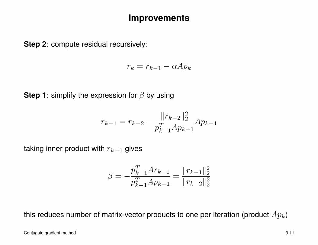
Improvements
Step 2: compute residual recursively:
rk = rk−1 − αApk
Step 1: simplify the expression for β by using
rk−1 = rk−2 −‖rk−2‖22
pTk−1Apk−1Apk−1
taking inner product with rk−1 gives
β = −pTk−1Ark−1
pTk−1Apk−1=‖rk−1‖22‖rk−2‖22
this reduces number of matrix-vector products to one per iteration (product Apk)
Conjugate gradient method 3-11
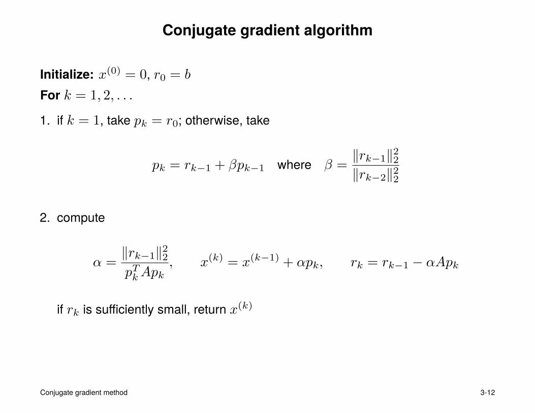
Conjugate gradient algorithm
Initialize: x(0) = 0, r0 = b
For k = 1, 2, . . .
1. if k = 1, take pk = r0; otherwise, take
pk = rk−1 + βpk−1 where β =‖rk−1‖22‖rk−2‖22
2. compute
α =‖rk−1‖22pTkApk
, x(k) = x(k−1) + αpk, rk = rk−1 − αApk
if rk is sufficiently small, return x(k)
Conjugate gradient method 3-12
Outline
• conjugate gradient method for linear equations
• convergence analysis
• conjugate gradient method as iterative method
• applications in nonlinear optimization
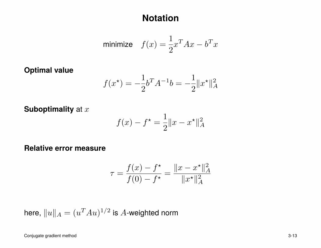
Notation
minimize f(x) =1
2xTAx− bTx
Optimal valuef(x?) = −1
2bTA−1b = −1
2‖x?‖2A
Suboptimality at xf(x)− f? =
1
2‖x− x?‖2A
Relative error measure
τ =f(x)− f?
f(0)− f?=‖x− x?‖2A‖x?‖2A
here, ‖u‖A = (uTAu)1/2 is A-weighted norm
Conjugate gradient method 3-13
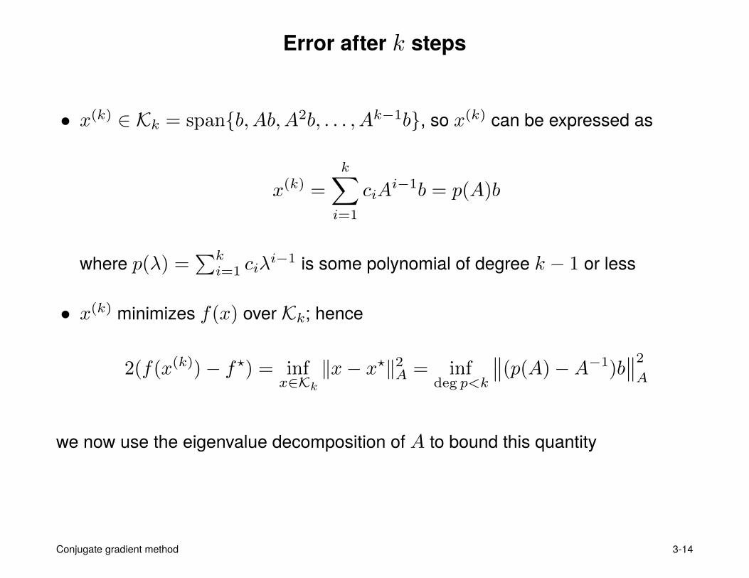
Error after k steps
• x(k) ∈ Kk = span{b, Ab,A2b, . . . , Ak−1b}, so x(k) can be expressed as
x(k) =
k∑i=1
ciAi−1b = p(A)b
where p(λ) =∑ki=1 ciλ
i−1 is some polynomial of degree k − 1 or less
• x(k) minimizes f(x) over Kk; hence
2(f(x(k))− f?) = infx∈Kk
‖x− x?‖2A = infdeg p<k
∥∥(p(A)−A−1)b∥∥2
A
we now use the eigenvalue decomposition of A to bound this quantity
Conjugate gradient method 3-14
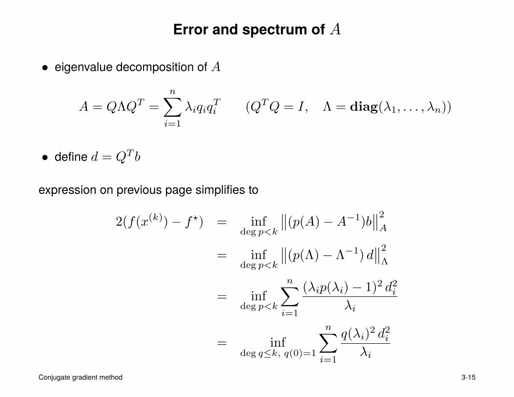
Error and spectrum of A
• eigenvalue decomposition of A
A = QΛQT =
n∑i=1
λiqiqTi (QTQ = I, Λ = diag(λ1, . . . , λn))
• define d = QT b
expression on previous page simplifies to
2(f(x(k))− f?) = infdeg p<k
∥∥(p(A)−A−1)b∥∥2
A
= infdeg p<k
∥∥(p(Λ)− Λ−1) d∥∥2
Λ
= infdeg p<k
n∑i=1
(λip(λi)− 1)2 d2i
λi
= infdeg q≤k, q(0)=1
n∑i=1
q(λi)2 d2
i
λi
Conjugate gradient method 3-15
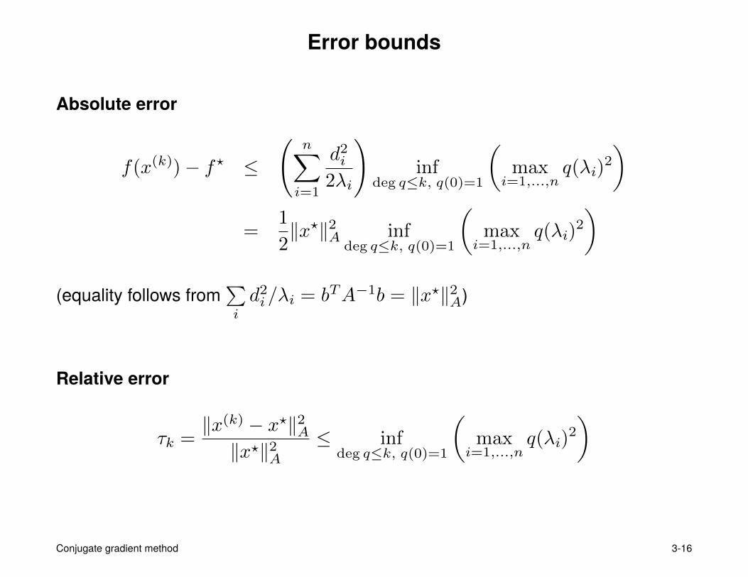
Error bounds
Absolute error
f(x(k))− f? ≤
(n∑i=1
d2i
2λi
)inf
deg q≤k, q(0)=1
(max
i=1,...,nq(λi)
2
)
=1
2‖x?‖2A inf
deg q≤k, q(0)=1
(max
i=1,...,nq(λi)
2
)
(equality follows from∑i
d2i/λi = bTA−1b = ‖x?‖2A)
Relative error
τk =‖x(k) − x?‖2A‖x?‖2A
≤ infdeg q≤k, q(0)=1
(max
i=1,...,nq(λi)
2
)
Conjugate gradient method 3-16
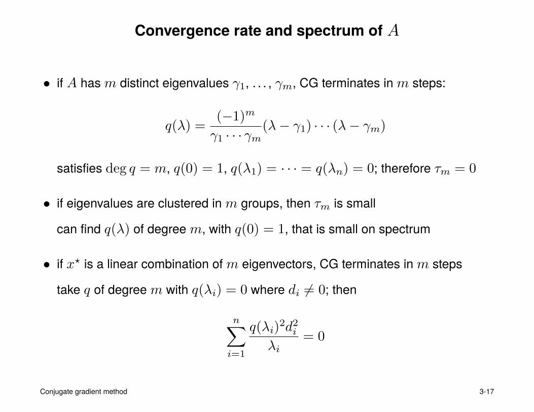
Convergence rate and spectrum of A
• if A hasm distinct eigenvalues γ1, . . . , γm, CG terminates inm steps:
q(λ) =(−1)m
γ1 · · · γm(λ− γ1) · · · (λ− γm)
satisfies deg q = m, q(0) = 1, q(λ1) = · · · = q(λn) = 0; therefore τm = 0
• if eigenvalues are clustered inm groups, then τm is small
can find q(λ) of degreem, with q(0) = 1, that is small on spectrum
• if x? is a linear combination ofm eigenvectors, CG terminates inm steps
take q of degreem with q(λi) = 0 where di 6= 0; then
n∑i=1
q(λi)2d2i
λi= 0
Conjugate gradient method 3-17
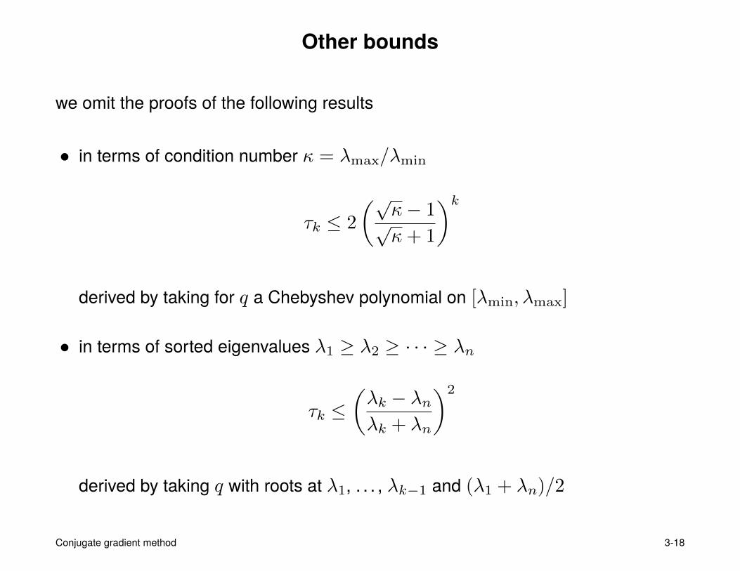
Other bounds
we omit the proofs of the following results
• in terms of condition number κ = λmax/λmin
τk ≤ 2
(√κ− 1√κ+ 1
)k
derived by taking for q a Chebyshev polynomial on [λmin, λmax]
• in terms of sorted eigenvalues λ1 ≥ λ2 ≥ · · · ≥ λn
τk ≤(λk − λnλk + λn
)2
derived by taking q with roots at λ1, . . . , λk−1 and (λ1 + λn)/2
Conjugate gradient method 3-18
Outline
• conjugate gradient method for linear equations
• convergence analysis
• conjugate gradient method as iterative method
• applications in nonlinear optimization
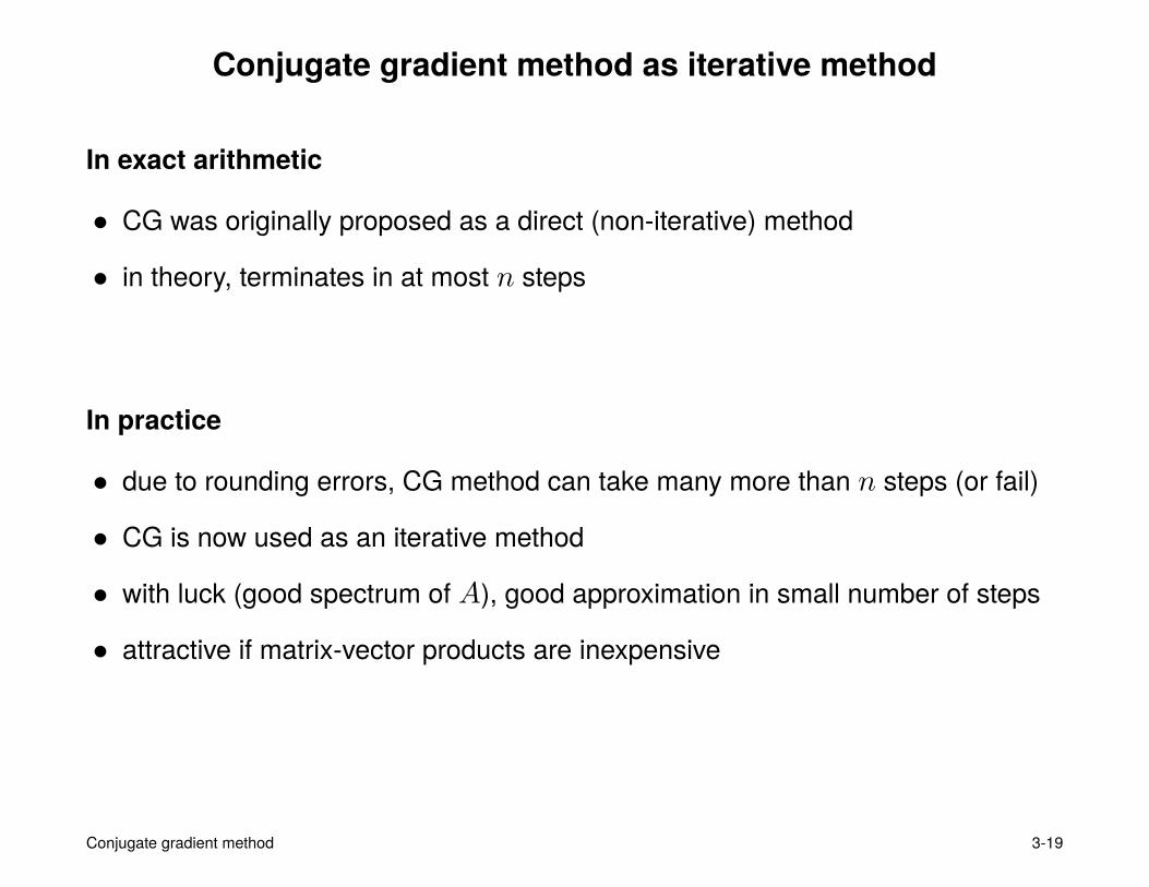
Conjugate gradient method as iterative method
In exact arithmetic
• CG was originally proposed as a direct (non-iterative) method
• in theory, terminates in at most n steps
In practice
• due to rounding errors, CG method can take many more than n steps (or fail)
• CG is now used as an iterative method
• with luck (good spectrum of A), good approximation in small number of steps
• attractive if matrix-vector products are inexpensive
Conjugate gradient method 3-19
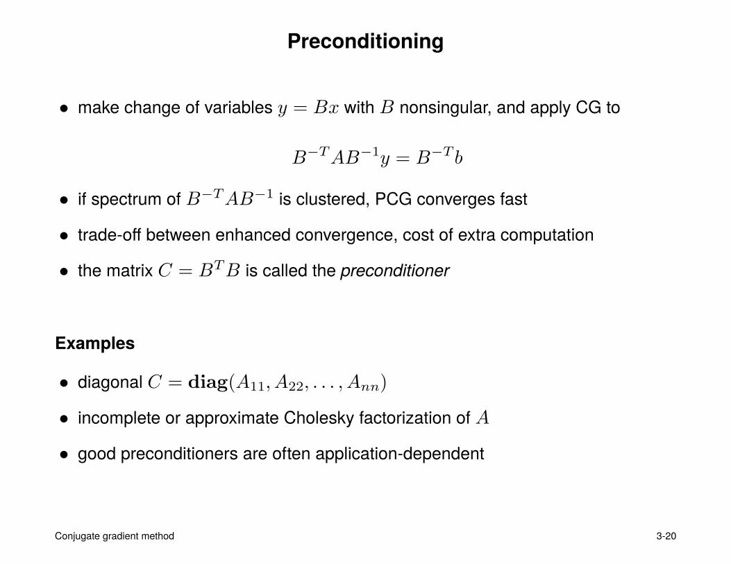
Preconditioning
• make change of variables y = Bx with B nonsingular, and apply CG to
B−TAB−1y = B−T b
• if spectrum of B−TAB−1 is clustered, PCG converges fast
• trade-off between enhanced convergence, cost of extra computation
• the matrix C = BTB is called the preconditioner
Examples
• diagonal C = diag(A11, A22, . . . , Ann)
• incomplete or approximate Cholesky factorization of A
• good preconditioners are often application-dependent
Conjugate gradient method 3-20
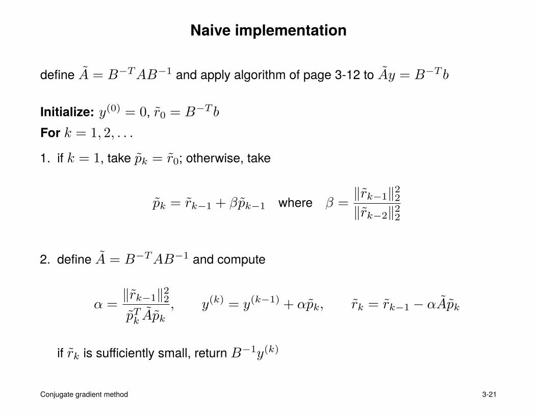
Naive implementation
define A = B−TAB−1 and apply algorithm of page 3-12 to Ay = B−T b
Initialize: y(0) = 0, r0 = B−T b
For k = 1, 2, . . .
1. if k = 1, take pk = r0; otherwise, take
pk = rk−1 + βpk−1 where β =‖rk−1‖22‖rk−2‖22
2. define A = B−TAB−1 and compute
α =‖rk−1‖22pTk Apk
, y(k) = y(k−1) + αpk, rk = rk−1 − αApk
if rk is sufficiently small, return B−1y(k)
Conjugate gradient method 3-21
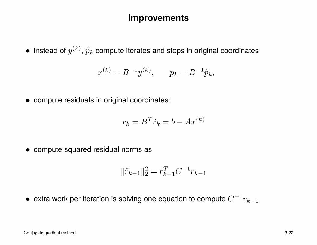
Improvements
• instead of y(k), pk compute iterates and steps in original coordinates
x(k) = B−1y(k), pk = B−1pk,
• compute residuals in original coordinates:
rk = BT rk = b−Ax(k)
• compute squared residual norms as
‖rk−1‖22 = rTk−1C−1rk−1
• extra work per iteration is solving one equation to compute C−1rk−1
Conjugate gradient method 3-22
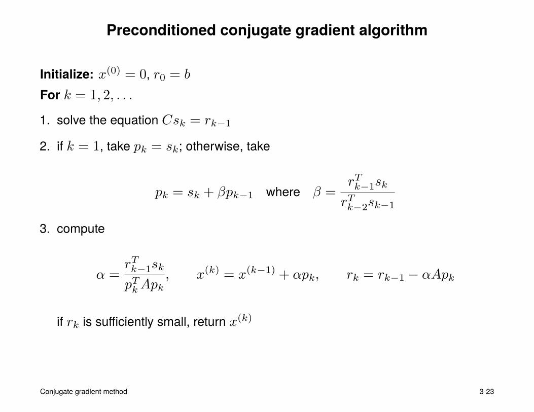
Preconditioned conjugate gradient algorithm
Initialize: x(0) = 0, r0 = b
For k = 1, 2, . . .
1. solve the equation Csk = rk−1
2. if k = 1, take pk = sk; otherwise, take
pk = sk + βpk−1 where β =rTk−1sk
rTk−2sk−1
3. compute
α =rTk−1sk
pTkApk, x(k) = x(k−1) + αpk, rk = rk−1 − αApk
if rk is sufficiently small, return x(k)
Conjugate gradient method 3-23
Outline
• conjugate gradient method for linear equations
• convergence analysis
• conjugate gradient method as iterative method
• applications in nonlinear optimization
Applications in optimization
Nonlinear conjugate gradient methods
• extend linear CG method to nonquadratic functions
• local convergence similar to linear CG
• limited global convergence theory
Inexact and truncated Newton methods
• use conjugate gradient method to compute (approximate) Newton step
• less reliable than exact Newton methods, but handle very large problems
Conjugate gradient method 3-24
Nonlinear conjugate gradient
minimize f(x)
(f convex and differentiable)
Modifications needed to extend linear CG algorithm of page 3-12
• replace rk = b−Ax(k) with −∇f(x(k))
• determine α by line search
Conjugate gradient method 3-25
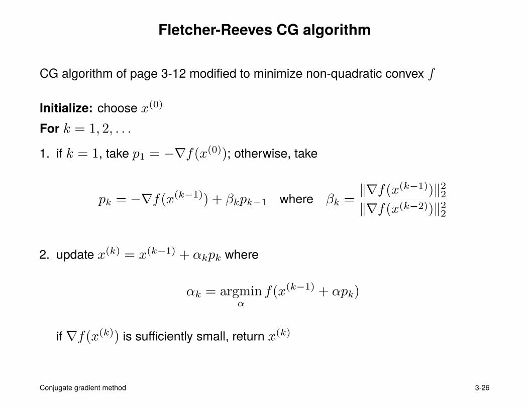
Fletcher-Reeves CG algorithm
CG algorithm of page 3-12 modified to minimize non-quadratic convex f
Initialize: choose x(0)
For k = 1, 2, . . .
1. if k = 1, take p1 = −∇f(x(0)); otherwise, take
pk = −∇f(x(k−1)) + βkpk−1 where βk =‖∇f(x(k−1))‖22‖∇f(x(k−2))‖22
2. update x(k) = x(k−1) + αkpk where
αk = argminα
f(x(k−1) + αpk)
if ∇f(x(k)) is sufficiently small, return x(k)
Conjugate gradient method 3-26
Some observations
Interpretation
• first iteration is a gradient step
• general update is gradient step with momentum term
x(k) = x(k−1) − αk∇f(x(k−1)) +αkβkαk−1
(x(k−1) − x(k−2))
• it is common to restart the algorithm periodically by taking a gradient step
Line search
• with exact line search, reduces to linear CG for quadratic f
• exact line search in step 2 implies ∇f(x(k))Tpk = 0
• therefore in step 1, pk is a descent direction at x(k−1):
∇f(x(k−1))Tpk = −‖∇f(x(k−1))‖22 < 0
Conjugate gradient method 3-27
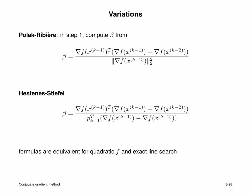
Variations
Polak-Ribière: in step 1, compute β from
β =∇f(x(k−1))T (∇f(x(k−1))−∇f(x(k−2)))
‖∇f(x(k−2))‖22
Hestenes-Stiefel
β =∇f(x(k−1))T (∇f(x(k−1))−∇f(x(k−2)))
pTk−1(∇f(x(k−1))−∇f(x(k−2)))
formulas are equivalent for quadratic f and exact line search
Conjugate gradient method 3-28
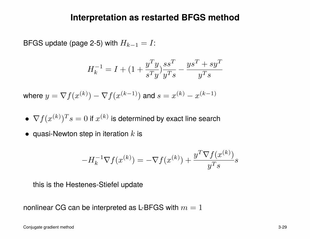
Interpretation as restarted BFGS method
BFGS update (page 2-5) with Hk−1 = I :
H−1k = I + (1 +
yTy
sTy)ssT
yTs− ys
T + syT
yTs
where y = ∇f(x(k))−∇f(x(k−1)) and s = x(k) − x(k−1)
• ∇f(x(k))Ts = 0 if x(k) is determined by exact line search
• quasi-Newton step in iteration k is
−H−1k ∇f(x(k)) = −∇f(x(k)) +
yT∇f(x(k))
yTss
this is the Hestenes-Stiefel update
nonlinear CG can be interpreted as L-BFGS withm = 1
Conjugate gradient method 3-29
References
• S. Boyd, Lecture notes for EE364b, Convex Optimization II.
• G. H. Golub and C. F. Van Loan, Matrix Computations (1996), chapter 10.
• J. Nocedal and S. J. Wright, Numerical Optimization (2006), chapter 5.
• H. A. van der Vorst, Iterative Krylov Methods for Large Linear Systems (2003).
Conjugate gradient method 3-30


![The Conjugate Gradient Method...Conjugate Gradient Algorithm [Conjugate Gradient Iteration] The positive definite linear system Ax = b is solved by the conjugate gradient method](https://img.pdfslide.us/doc/110x75/5e95c1e7f0d0d02fb330942a/the-conjugate-gradient-method-conjugate-gradient-algorithm-conjugate-gradient.jpg)