Electromagnetics Laboratory Report Series

Espoo, April 2004 REPORT 434

SOLVING ELECTROMAGNETIC BOUNDARY PROBLEMS WITH

EQUIVALENCE METHODS

Jari J. Hänninen

AB TEKNILLINEN KORKEAKOULUTEKNISKA HÖGSKOLANHELSINKI UNIVERSITY OF TECHNOLOGYTECHNISCHE UNIVERSITÄT HELSINKIUNIVERSITE DE TECHNOLOGIE D’HELSINKI

−0.084

−0.084

−0.079

−0.079−0.074

−0.074

−0.069

−0.069−0.064

−0.064

−0.059

−0.059

−0.054

−0.054

−0.049 −0.049

−0.044

−0.044−0

.044−0.039

−0.039

−0.039

−0.034

−0.034

−0.034

−

−0.029−0.029

29−0.

−0.024−0.024

−0.

024

−0.019

−0.019

−0.019

−0.014

−0.014 −0.014

−0.014−0.0090.00

−0.0

−0.009

−0.

004

−0.004

Electromagnetics Laboratory Report Series

Espoo, April 2004 REPORT 434

SOLVING ELECTROMAGNETIC BOUNDARY PROBLEMS WITH

EQUIVALENCE METHODS

Jari J. Hänninen

Dissertation for the degree of Doctor of Science in Technology to be presented with due permission of

the Department of Electrical and Communications Engineering, Helsinki University of Technology, for

public examination and debate in Auditorium S4 at Helsinki University of Technology (Espoo,

Finland) on the 7th of May, 2004, at 12 noon.

Helsinki University of Technology

Department of Electrical and Communications Engineering

Electromagnetics Laboratory

Distribution:

Helsinki University of Technology

Electromagnetics Laboratory

P.O. Box 3000

FIN-02015 HUT

Tel. +358 9 451 2264

Fax +358 9 451 2267

ISBN 951-22-7080-3

ISSN 1456-632X

Picaset Oy

Helsinki 2004

Abstract

A basic problem in electromagnetics involves solving the Maxwell equations in anon-empty space, i.e. in a space with interfaces or boundaries. In this dissertation thewanted electromagnetic fields are searched via equivalence methods: a full electromag-netic problem is transformed to a simpler solvable form, or the solution is an equivalentsource, or both. The chosen transformations result to two slightly different transmis-sion line formulations or to Kelvin inversion (inversion in a sphere). The equivalentsource is typically an image source. The included cases are 1) a planar multilayer chiralstructure, 2) a conducting earth under a current source, 3) a sphere in an isotropicor bi-isotropic space, and 4) three types of anisotropic half-space–planar boundary orhalf-space problems. The first two cases (three papers) are time-dependent problemsand the latter two (four papers) statics or quasi-statics. In each case the solution meth-odology is presented, the solutions are written, and the implications and limitationsare discussed.

Keywords:

equivalence method — equivalent source — electromagnetic image principle —Kelvin inversion — bi-isotropic medium — anisotropic medium —

exact image theory (EIT) — geomagnetically induced currents (GIC) —transmission line — electrostatics

iii

O glaube, mein Herz, o glaube: Es geht dir nichts verloren!

Dein ist, ja dein, was du gesehnt!

Dein, was du geliebt, was du gestritten!

O glaube: Du wardst nicht umsonst geboren!

Hast nicht umsonst gelebt, gelitten!

Gustav Mahler

in the fifth movement of his Second Symphonytoisen sinfoniansa viidennessa osassa

iv

Thanks

For ideas and fruitful collaboration: Professor Ismo V. Lindell, supervisor of the thesis;Professor Keijo Nikoskinen, my trusted colleague.

For swiftness: Docent Esko Eloranta and D.Sc.(Tech) Murat Ermutlu,pre-examiners of the thesis.

For employment and funding: Professor Ari Sihvola, Head of Laboratory;Graduate School of Applied Electromagnetics.

For assistance in practical matters: Katrina Nykanen, Secretary of Laboratory.For enduring my jokes: M.Sc.(Tech) Sami Ilvonen, my friend sharing the workroom.For cheerful moments: my fellow post-graduates; my dear friends.For participation: the rest of the Laboratory personnel;

other involved persons not yet mentioned.For life: my beloved parents Paavo and Liisa.

Jari J. HanninenEspoo, Finland, 16th April 2004

Kiitokset

Ideoista ja tuloksekkaasta yhteistyosta: vaitoskirjatyon valvoja professori Ismo V. Lindell;luottokollegani professori Keijo Nikoskinen.

Joutuisuudesta: vaitoskirjan esitarkastajat dosentti Esko Eloranta ja TkT Murat Ermutlu.Tyosuhteesta ja rahoituksesta: laboratorion johtaja professori Ari Sihvola;

sovelletun sahkomagnetiikan tutkijakoulu.Kaytannon asiain hoidosta: laboratorion sihteeri Katrina Nykanen.Vitsieni kestamisesta: tyohuoneystavani DI Sami Ilvonen.Hilpeista hetkista: jatko-opiskelutoverini; armaat ystavani.Osallistumisesta: loput virkaveljeni laboratoriossa;

viela mainitsemattomat muut mukanaolleet.Elamasta: rakkaat vanhempani Paavo ja Liisa.

Jari J. HanninenEspoossa 16. huhtikuuta 2004

v

List of publications

[P1] Oksanen, M.I., Hanninen, J. & Tretyakov, S.A. “Vector circuit method forcalculating reflection and transmission of electromagnetic waves in multilayer chiralstructures”. IEE Proceedings H, Microwaves, Antennas and Propagation, 138(1991)6,p. 513–520.

[P2] Lindell, I.V. & Hanninen, J.J. “Static image principle for the sphere in isotropicor bi-isotropic space”. Radio Science, 35(2000)3, p. 653–660.

[P3] Lindell, I.V., Hanninen, J.J. & Pirjola, R. “Wait’s complex-image principlegeneralized to arbitrary sources”. IEEE Transactions on Antennas and Propagation,48(2000)10, p. 1618–1624.

[P4] Hanninen, J.J., Pirjola, R.J. & Lindell, I.V. “Application of the EIT to studiesof ground effects of space weather”. Geophysical Journal International, 151(2002)-,p. 534–542.

[P5] Lindell, I.V., Hanninen, J.J. & Nikoskinen, K.I. “Electrostatic image theoryfor an anisotropic boundary”. IEE Proceedings—Science, Measurement & Technology,accepted for publication.

[P6] Hanninen, J.J., Lindell, I.V. & Nikoskinen, K.I. “Electrostatic image theoryfor an anisotropic boundary of an anisotropic half-space”. Progress in ElectromagneticsResearch, 47(2004)-, p. 235–262.

[P7] Hanninen, J.J., Nikoskinen, K.I. & Lindell, I.V. Electrostatic image theory fortwo anisotropic half-spaces. (Electromagnetics Laboratory Report Series, Report 428).Espoo, Finland 2004: Helsinki University of Technology, Electromagnetics Laboratory.(Submitted in shorter form to Electrical Engineering (Archiv fur Elektrotechnik).)

Contribution of the author

In all the papers the first author was responsible for the manuscript.The papers [P4], [P6], and [P7] were mainly done by the author of the thesis; this included

developing the theory, presenting it, and verifying the results.Papers [P1]–[P3] and [P5] were the result of collaboration of the authors; the thesis author

took especially care of the numerical verifications (where applicable).

vi

1

1 Introduction

Take an empty universe (in the classical sense), set a charge distribution “somewhere,” andexpress the density and time-dependence of that charge distribution as a function of positionand time. Because electromagnetic field theory has long since been equipped with Greenfunctions for free space, it should be straightforward to calculate the fields emanating fromthis source, be the source truly time-varying or static.

In principle the sketched process could be applied to a non-empty universe like ours.Instead of having free space we now have boundaries (changes in material parameters), butwe could try to construct a Green function—the field of a point source—for the geometryinvolved and determine the electromagnetic field for all possible sources by integration. Thebad news is that it is extremely difficult to construct Green functions for general boundaryproblems. Some detour is necessary. . .

An ‘equivalence method’ in electromagnetics is an indirect method with which it is pos-sible to obtain a solution to the original electromagnetic problem which may otherwise bedifficult or impossible to solve. As will be seen later, the equivalence may mean utilisingsome mathematical apparatus to write the equations of the problem in a new “language”(physical space–Maxwell equations vs. Fourier-space–transmission line equations), or it maymean that an obtained result (e.g., a reflection image source), after proper application, givescorrect electromagnetic fields in (some part of) the physical space under study. These classesmay also be combined, giving two instances or levels of equivalence inside one problem.

This Summary first collects some common electromagnetic formulas. The seven includedpapers are then scrutinised in Section 5 to show various equivalence methods in action, bothon the problem-solving level and on the result level. The aim is to give a general view ofequivalence methods and also to discuss some aspects of the results, though this is mainlycovered by the papers themselves.

Among solution-level equivalence methods can be counted the use of different transmis-sion line analogies [P1] and [P5]–[P7], and Kelvin inversion [P2]. On the result level we seereflection or transmission coefficients in [P1], or equivalent sources (images) in [P2]–[P7]. In[P1] we have the plane wave excitation disguised as an equivalent source!

2 Electromagnetic formulation

2.1 Maxwell equations

The classical electromagnetic field theory—or electrodynamics, as it is also called—is builtupon the four Maxwell equations [D1, (3.1)–(3.4)]

∇× E(r, t) = − ∂

∂tB(r, t) (Faraday’s law), (D1)

∇× H(r, t) = J(r, t) +∂

∂tD(r, t) (Ampere’s law), (D2)

∇ · D(r, t) = (r, t) (Gauss’ law), and (D3)

∇ · B(r, t) = 0. (D4)

Here E(r, t) is the electric field (strength), D(r, t) is the electric flux density (or electricdisplacement), H(r, t) is the magnetic field (strength), and B(r, t) is the magnetic fluxdensity (or magnetic induction). The sources of the electromagnetic fields are the current

2

density J(r, t) and the electric charge density (r, t). Equation (D4) is usually left unnamedbecause free magnetic charges (monopoles) have not been observed (although Dirac’s theory[D2] favours their existence). However, it is occasionally useful to symmetrize the right-hand sides of the equations by adding a magnetic charge density m(r, t) to (D4) and acorresponding negative magnetic current density −Jm(r, t) to (D1).

We can apply the Fourier transformation pair

F (r, ω) =

∫

∞

−∞

f(r, t)e−jωt dt ↔ f(r, t) =1

2π

∫

∞

−∞

F (r, ω)ejωt dω (D5)

to Maxwell equations to obtain equations without explicit time derivatives (magnetic chargesagain omitted):

∇× E(r, ω) = −jωB(r, ω), (D6)

∇× H(r, ω) = J(r, ω) + jωD(r, ω), (D7)

∇ · D(r, ω) = (r, ω), (D8)

∇ · B(r, ω) = 0. (D9)

All quantities are now complex. By the left-hand equation of (D5) we see that F (r,−ω) =F ∗(r, ω) because physical time-dependent fields are real.

If we assume that the electromagnetic sources (and thus the fields) have a single-frequencysinusoidal time dependence, a function f(r, t) is related to the complex function F (r) by

f(r, t) = ℜ{

F (r)ejωt}

, (D10)

where F (r) is a Fourier-transformed quantity (phasor, complex vector) without the negativefrequencies. In this time-harmonic case we usually write the Maxwell equations in shortform, without the argument ω, i.e. ∇× E(r) = −jωB(r), etc. From now on we employ theshort form.—In papers [P1], [P3] and [P4] time-harmonic fields are discussed.

It is easy to see from equations (D7) and (D8) that ∇· J(r) = −jω(r), so we do not needto use (D8) explicitly when solving time-harmonic problems. Likewise, taking the divergenceof equation (D6) gives us equation (D9) directly.

Electric and magnetic quantities decouple if there is no time dependence, ∂f(r, t)/∂t ≡ 0or ω ≡ 0. We then get electrostatics,

∇× E(r) = 0, (D11)

∇ · D(r) = (r), (D12)

or magnetostatics

∇× H(r) = J(r), (D13)

∇ · B(r) = 0. (D14)

It should be observed that ∇· J(r) = 0, which means that there is no accumulation of charge(in time) anywhere. Under static conditions all quantities are real. Also, in electrostaticswe have the possibility of using electric potential φ(r), which gives the electric field viaE(r) = −∇φ(r).—Papers [P2] and [P5]–[P7] handle statics or quasistatics.

3

2.2 Constitutive relations

In the Maxwell equations we have 12 unknowns and only six independent equations—(D3)and (D4) are obtainable from (D2) and (D1), respectively. So, we need to relate the fieldvectors E, B, H, and D with additional constraints to solve field problems. This is done bytaking the effects of material media into account with constitutive relations. For example,in a linear bianisotropic medium we have [D1, p. 54]

D = ¯ǫ · E + ¯ξ · H, (D15)

B = ¯ζ · E + ¯µ · H. (D16)

The exact physical behaviour of a medium is hidden inside the dyadic medium parameters¯ǫ (permittivity), ¯ξ, ¯ζ (magnetoelectric dyadics), and ¯µ (permeability). (Here the mediumis assumed to be local and non-dispersive.) We can also relate the electric field and currentdensity via Ohm’s law:

J = ¯σ · E, (D17)

where ¯σ is the conductivity dyadic.

If the medium dyadics are multiples of the unit dyadic ¯I, i.e. ¯ǫ = ǫI, ¯ξ = ξ¯I, ¯ζ = ζ¯I,and ¯µ = µ¯I, the medium is said to be bi-isotropic. This kind of medium is encounteredin paper [P2]. If we simplify the material even further, we get an isotropic chiral mediumhaving ξ = −jκ

√µ0ǫ0 and ζ = jκ

√µ0ǫ0. Chiral materials are discussed in paper [P1]. If

the chirality parameter κ is zero, we end up with an “ordinary” isotropic medium with theconstitutive equations

D = ǫ E, (D18)

B = µ H. (D19)

In free space ǫ = ǫ0 and µ = µ0. This is the type of medium met in papers [P3], [P4],and [P5].

The bi-isotropic material parameters ¯ξ and ¯ζ are nonzero only under time-varying con-ditions. In electrostatics we can nevertheless have anisotropic materials, described by therelation

D = ¯ǫ · E. (D20)

This is something we look at in papers [P6] and [P7]. Under dynamic conditions the mediumrelation would look the same but the medium dyadic would not necessarily be symmetricand positive definite, as it is in electrostatics [D3, §13 & §21].

After adding the constitutive relations we have taken one step forward in solving theMaxwell equations. What are needed to finish the process are the interface conditions,which we discuss next.

2.3 Interface conditions

In the previous section we considered media that could be assumed to be homogeneous overat least some small region of space. If the medium parameters are discontinuous, for example,there is a planar or spherical surface separating two different dielectrics, the electromagneticfields will also have discontinuities. These discontinuities can be taken into account with the

4

I(z) I(z)+dI(z)

z

u(z) dz l dz r dz

i(z) dz g dz

z z+dz

U(z) U(z)+dU(z)c dz

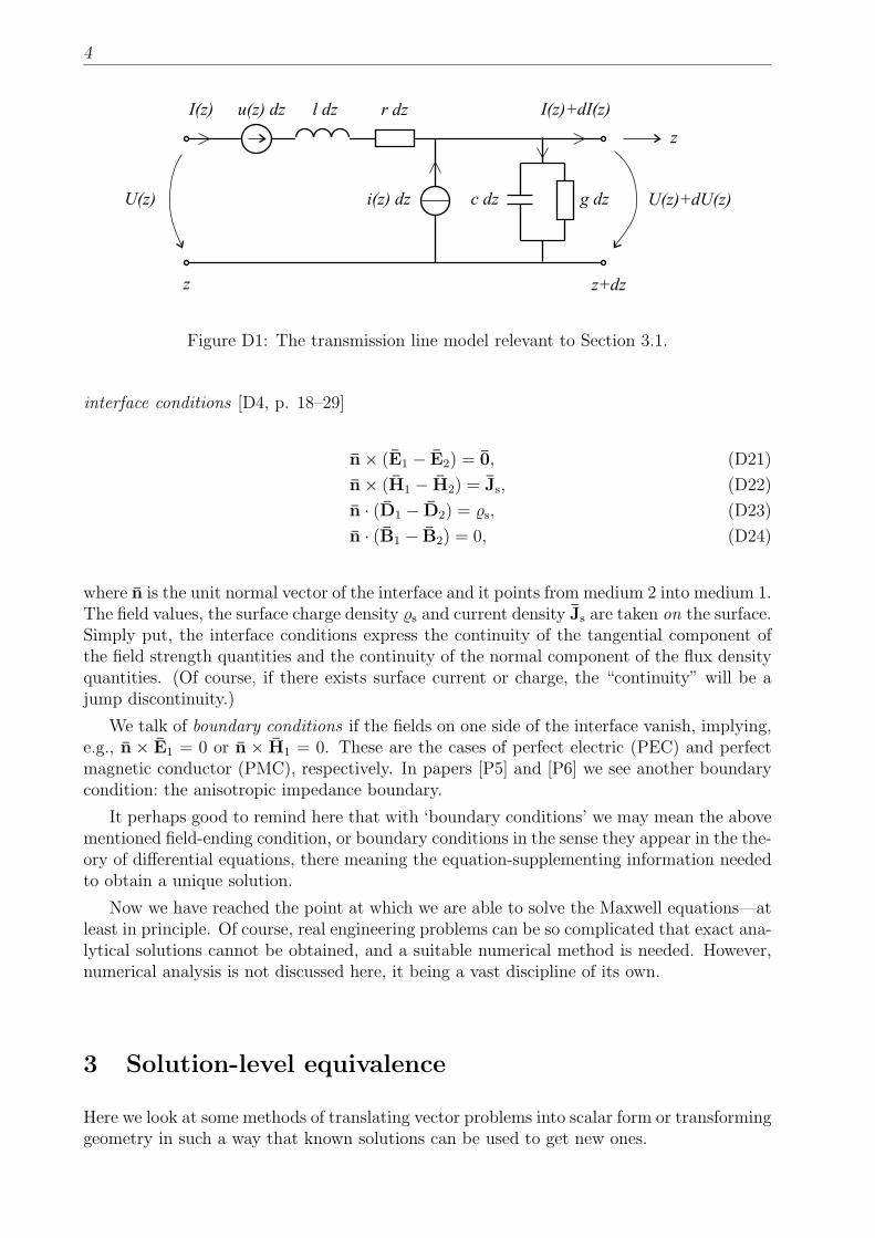
Figure D1: The transmission line model relevant to Section 3.1.

interface conditions [D4, p. 18–29]

n × (E1 − E2) = 0, (D21)

n × (H1 − H2) = Js, (D22)

n · (D1 − D2) = s, (D23)

n · (B1 − B2) = 0, (D24)

where n is the unit normal vector of the interface and it points from medium 2 into medium 1.The field values, the surface charge density s and current density Js are taken on the surface.Simply put, the interface conditions express the continuity of the tangential component ofthe field strength quantities and the continuity of the normal component of the flux densityquantities. (Of course, if there exists surface current or charge, the “continuity” will be ajump discontinuity.)

We talk of boundary conditions if the fields on one side of the interface vanish, implying,e.g., n × E1 = 0 or n × H1 = 0. These are the cases of perfect electric (PEC) and perfectmagnetic conductor (PMC), respectively. In papers [P5] and [P6] we see another boundarycondition: the anisotropic impedance boundary.

It perhaps good to remind here that with ‘boundary conditions’ we may mean the abovementioned field-ending condition, or boundary conditions in the sense they appear in the the-ory of differential equations, there meaning the equation-supplementing information neededto obtain a unique solution.

Now we have reached the point at which we are able to solve the Maxwell equations—atleast in principle. Of course, real engineering problems can be so complicated that exact ana-lytical solutions cannot be obtained, and a suitable numerical method is needed. However,numerical analysis is not discussed here, it being a vast discipline of its own.

3 Solution-level equivalence

Here we look at some methods of translating vector problems into scalar form or transforminggeometry in such a way that known solutions can be used to get new ones.

5

3.1 The transmission line model

We take a length dz of a lossy transmission line, Figure (D1). Using circuit theory we havethe two time-harmonic equations

U(z) + u(z) dz − (jωl + r) dz − (U(z) + dU(z)) = 0, (D25)

I(z) − (I(z) + dI(z)) + i(z) dz − (jωc + g) dz · (U(z) + dU(z)) = 0. (D26)

After writing out the differentials, i.e. dI(z) = ∂zI(z) dz etc., and neglecting higher orderdifferentials we get the transmission line equation

(

∂z (jωl + r)(jωc + g) ∂z

)(

U(z)I(z)

)

=

(

u(z)i(z)

)

. (D27)

If we can cast vector equations into scalar form, which has for example been done in papers[P5]–[P7] by using the two-dimensional Fourier transformation, we can use the full set oftools from transmission line theory to determine reflection and transmission coefficients invarious geometries.

Paper [P2] has a different approach: there a vector circuit has been used. For furtherreference the paper itself should be studied.

3.2 Affine transformation

In paper [P6] the image source is constructed via the transmission line equivalence. Theresult of [P5] at our disposal, we could have used affine transformation to turn the isotropicpermittivity of the upper half-space into an anisotropic one, giving essentially the same endresult as in [P6]. However, the derivation is quite long, and though in paper [P6, (53)] (and[P7]) an affine transformation is being used, it takes place deep inside the formulation. Herea from-the-start affine transformation method is outlined.

We start with the anisotropic problem and look for an affine transformation that trans-forms the anisotropic half-space into an isotropic one. This process gives us a dictionary formoving back and forth between the two spaces. Then, using the existing results in [P5], wecould find the image source of a point source above an anisotropic impedance surface andtransform the image, the boundary, and the geometry into our anisotropic space. It shouldbe noted that for practical purposes we should apply the affine transformation twice—firstto transform the anisotropic case isotropic (‘forward’) and then back (‘inverse’). Here weassume, for the sake of clarity, that the first transformation has been carried out already.

3.2.1 Transforming the equations

We use the electrostatic Maxwell equations (D11) and (D12), and the constitutive relation(D20). The general permittivity dyadic ¯ǫr is, of course, symmetric and positive definite.

From now on we denote quantities of the isotropic case with primes (and the anisotropiccase without). The Cartesian unit vectors (ux, uy, uz) coincide with the isotropic geometrybut are unprimed because they form the invariant coordinate framework. (Dyadic notationwould allow us to avoid using coordinates, but illustrating the affine transformation withoutany coordinate system would be difficult.)

First we seek the transformation ∇ ↔ ∇′. Utilising (D12) and requiring the Maxwell

6

equations to hold in both spaces we get

ǫ0∇ · ¯ǫr · E(r) = (r)

⇔ ǫ0∇ · ¯ǫ1/2r · ¯ǫ1/2

r · E(r) = (r)

⇔ ǫ0 (ǫ1/2r · ∇) · (ǫ1/2

r · E(r)) = (r)

⇔ ǫ0∇′ · E′(r′) = ′(r′) (D28)

if we identify

∇′ = ¯ǫ1/2r · ∇ ↔ ∇ = ¯ǫ−1/2

r · ∇′, (D29)

E′(r′) = ¯ǫ1/2r · E(r) ↔ E(r) = ¯ǫ−1/2

r · E′(r′). (D30)

From (D28) it is immediately seen that we have got an isotropic medium in the primedspace:

D′(r′) = ǫ0E′(r′), (D31)

∇′ · D′(r′) = ′(r′). (D32)

The charge density has, of course, a different-looking expression in each space but otherwiseit is an invariant, i.e. (r) = ′(r′). See below for the further discussion of the sources.

Transformation r ↔ r′ is obtained from (D29) and the identity ¯I = ∇r = ∇′r′:

¯I = ∇′r′ = (ǫ1/2r · ∇)r′ = ∇(ǫ1/2

r · r′) = ∇r. (D33)

This gives the pair (which could have been used to define the affine transformation)

r′ = ¯ǫ−1/2r · r ↔ r = ¯ǫ1/2

r · r′. (D34)

Finally, before proceeding to the handling of boundary conditions, let us verify the pre-vious results by applying the identity ( ¯A · a) × ( ¯A · b) = ¯A(2) · (a× b) = 1

2( ¯A ×

ׯA) · (a× b)

to (D11), giving us

∇×E(r) = (ǫ−1/2r ·∇′)× (ǫ−1/2

r ·E′(r′)) = (ǫ−1/2r )(2) ·(∇′×E′(r′)) = 0 ⇔ ∇′×E′(r′) = 0.

(D35)So, with the chosen affine transformation the Maxwell equations remain intact.

3.2.2 Transforming the sources and boundary conditions

The impedance boundary condition of the anisotropic surface z = 0 of the isotropic half-space z > 0 is

n′ · D′(ρ′) = −∇′

t · Ψ′

s(ρ′) = −ǫ0∇′

t · ¯ζ ′

r · E′

t(ρ′). (D36)

The surface impedance dyadic ¯ζ ′

r is symmetric and positive definite; it can be expressed

as ¯ζ ′

r = uxuxζ′

x + uyuyζ′

y without loss of generality. In addition, ρ′ = uxx′ + uyy

′ is thetransverse position vector, and subscript ‘t’ denotes ‘transverse’ with respect to z. QuantityΨ

′

s(ρ′) is the electric surface flux density. The surface normal n′ of the anisotropic boundary

of the isotropic case coincides with uz.Because ρ′, ∇′

t, and E′

t transform as r′, ∇′, and E′, respectively, the boundary condi-tion (D36) transforms as

n′ · D′(ρ′) = −ǫ0∇′

t · ¯ζ ′

r · E′

t(ρ′)

⇔ n′ · (ǫ0¯ǫ1/2r · Et(ρ)) = −ǫ0 (ǫ

1/2r · ∇t) · ¯ζ ′

r · (ǫ1/2r · Et(ρ))

⇔ (n′ · ¯ǫ−1/2r ) · (ǫ0¯ǫr · Et(ρ)) = −ǫ0∇t · (ǫ1/2

r · ¯ζ ′

r · ¯ǫ1/2r ) · Et(ρ)

⇔ n · D(ρ) = −ǫ0∇t · ¯ζr · Et(ρ). (D37)

7

We have required |n| = 1, and can thus identify

ρ = ¯ǫ1/2r · ρ′ ↔ ρ′ = ¯ǫ−1/2

r · ρ , (D38)

n =¯ǫ−1/2r · n′

√

n′ · ¯ǫ−1r · n′

=¯ǫ−1/2r · uz

√

uz · ¯ǫ−1r · uz

↔ n′ =¯ǫ

1/2r · n√n · ¯ǫr · n

, and (D39)

¯ζr =¯ǫ

1/2r · ¯ζ ′

r · ¯ǫ1/2r

√

n′ · ¯ǫ−1r · n′

=¯ǫ

1/2r · ¯ζ ′

r · ¯ǫ1/2r

√

uz · ¯ǫ−1r · uz

↔ ¯ζ ′

r =¯ǫ−1/2r · ¯ζr · ¯ǫ−1/2

r√n · ¯ǫr · n

. (D40)

As the transforming of n′ to n suggests, the anisotropic surface of the anisotropic case, ingeneral, becomes slanted with respect to the anisotropic surface of the isotropic case (thesurfaces are defined as n · r = 0 and n′ · r′ = 0, respectively). We could use n and, forexample, the transformation of ux to define (after some steps) a coordinate system local tothe unprimed system, similar to the Cartesian coordinate system of the isotropic case.

Finally we construct the very simple transformation of sources by using the invarianceof charges:

′(r′) = (r) = (ǫ1/2r · r′) = ′ (ǫ−1/2

r · r). (D41)

As stated earlier, we consider the case of a point charge in the isotropic space. Our chargedensity is therefore ′(r′) = Q′δ(ρ′)δ(z − z′0) = Q′δ(r′ − r′0), i.e. we have a charge Q′ inr′0 = uzz

′

0 (z′0 > 0). Applying (D41), we get for the anisotropic space

′(r′) = Q′δ(ǫ−1/2r · r − uzz

′

0) = Q′δ(

¯ǫ−1/2r · (r − ¯ǫ1/2

r · uzz′

0))

= Qδ(r − r0) = (r) (D42)

with

Q = Q′/

√

det(ǫ−1/2r ) ↔ Q′ = Q/

√

det(ǫ1/2r ), (D43)

r0 = ¯ǫ1/2r · r′0 =

(

¯ǫr · n√

uz · ¯ǫ−1r · uz

)

z′0 ↔ r′0 = ¯ǫ−1/2r · r0. (D44)

The delta function has been simplified with δ( ¯A· r) = δ(r)/ det ¯A, which holds for symmetricpositive definite dyadics. Transformation of the reflection image r ′(r′) in the isotropic spaceto an image in the anisotropic space is

r(r) = r ′(r′) = r ′ (ǫ−1/2r · r). (D45)

This step completes our dictionary; constructing the expression of the transformed reflectionimage would become next, but we end the demonstration of the technique here. The affinetransformation has been used, for example, in [D5].

3.3 Kelvin inversion

This is another method for changing the geometry. In paper [P2] Kelvin inversion is usedto determine image sources by inverting the outside of a sphere inside it. It would also bepossible to use a suitable chosen inversion sphere with respect to a wedge and obtain imagessources for a whole new class of geometries [D6].

4 Equivalent sources

The form of the Maxwell equations suggests that if we know the fields everywhere, we alsoknow the sources everywhere. But if we limit our scope only to a volume V , there may be

8

other sources which give the same fields in V . These sources will be called equivalent sources(with respect to V ), [D1, p. 165].

We start with a space with some obstacles (or interfaces or scatterers, as they might becalled) in it. We can solve for the radiation (statics included) of the original source in a spacewithout the interfaces, then find a suitable equivalent source (a combination of the originalsource and an auxiliary source) satisfying the boundary conditions, and finally calculate thefields from these two sources in the proper part of the again interfaceless (homogeneous)space. If the auxiliary source somehow resembles a geometric image of the original source,we would call it the image source, and the field arising from it the reflected field. Theuniqueness of the solutions of Maxwell equations (augmented with suitable boundary orradiation conditions) guarantees us the right answer (for a thorough discussion see Section 3.5of [D1]).

The classical example of the use of an image method is the problem of a point charge Q atheight h above an infinite PEC plane. The reflected field at the upper half-space is obtaineddirectly from the image source −Q at height h below the level of the PEC plane after thePEC plane has been removed, and the lower half-space has been filled with the medium ofthe upper half-space. A homogeneous-space Green function is needed to determine the fieldsof the image source—the difficult task of finding the geometry-matched Green function isavoided.

The Huygens’ principle is another, yet slightly different, example of equivalent sources.In it the original sources are discarded altogether after the equivalent sources on a pre-defined surface have been obtained; fields inside the surface are solely determined by thesesources. For an elegant derivation of the Huygens’ principle see [D7].—Multipole expansionsrepresenting arbitrary sources also belong to the class of equivalent sources.

It should be noted that if we subtract the field of the equivalent source from the field ofthe original source, we naturally get zero field in V . The sum of the original source with thenegative equivalent source is called a nonradiating source with respect to V .

Unfortunately finding equivalent sources is not always possible. For example, the imageprinciple has so far been only used for some simple interface geometries like the plane (staticor time-harmonic case) or sphere (static case). On the other hand, when the image isavailable, it is an intuitively appealing expression of the solution, and mental pictures ofdifficult problems can be acquired with the aid of it. Some numerical difficulties can alsobe avoided; see, e.g., the discussion about the exact image theory (EIT) solution [D8] of theSommerfeld half-space problem.

5 Commentary of Papers [P1]–[P7]

5.1 Paper [P1]

Oksanen, M.I., Hanninen, J. & Tretyakov, S.A. “Vector circuit methodfor calculating reflection and transmission of electromagnetic waves in multilayerchiral structures”. IEE Proceedings H, Microwaves, Antennas and Propagation,138(1991)6, p. 513–520.

This paper is the oldest one and is therefore presented first. Also, the frequency range ofthe method is unlimited (as long as ω > 0); at the later papers we deal with low frequenciesor even with statics.

The article is a generalisation of another paper [1],1 in which the vector circuit method

1In Section 5 all references are to the paper in question, unless otherwise noted.

9

(VCM) was applied to one chiral slab. Now several slabs are stacked upon each other andthe reflection and transmission dyadics for the whole structure are determined. The benefitof using dyadic algebra is clear: both eigenpolarisations can be handled simultaneously, andthe results have a compact representation.

The setup of the problem is shown in Fig. 1. Tangential components are naturally takenalong the planar interfaces. By the “upper side” of the slab is actually meant the left side,and by the “lower side” the right side.

In addition to an equivalence in the solution process (the VCM), we have here an ex-tremely simple equivalent source: it is just two times the tangential component of the electricfield of the incoming plane wave and is interpreted as a vector voltage source for the vectortransmission line. The impedances of the transmission line sections are dyadics, and thetwo-port circuit has dyadic transfer parameters. The expressions for the elements of thematrix [¯a] are given in equations (8)–(11) for one slab and in equations (19)–(22) for thecombination of the two rightmost slabs; the total [¯a]-matrix is obtained by recursively ap-

plying equations (19)–(22) to all slabs. Equation (25) gives the input impedance ¯Zeq of the

whole structure. The ¯a, ¯Zc, and ¯Z′

c dyadics were derived by using a two-dimensional spatialFourier transformation on the plane of the slabs.

The reflection ( ¯Re) and transmission ( ¯Te) dyadics for the tangential electric fields aregiven by equations (30)–(32). The total reflected and transmitted electric fields for a TEincident wave are given in equations (39) and (40) and for a TM incident wave in equations(43) and (44). The reflection and transmission dyadics contain information about boththe co- and cross-polarisation behaviour of the incident wave. The analytical part and allnecessary formulas are ready by the end of Section 4.

Since the publication of this paper the research of chirality has produced new theoreticaland experimental results (see, e.g. [D9, D10, D11]); chiral materials have been seen to be lesssuperior than they once were thought to be. The physical realizability of the κ-parametersof this article should perhaps be checked one day—if not for the sake of science, then at leastfor the personal interest.

5.2 Paper [P2]

Lindell, I.V. & Hanninen, J.J. “Static image principle for the sphere inisotropic or bi-isotropic space”. Radio Science, 35(2000)3, p. 653–660.

The image principle for a PEC sphere and a (static) electric point charge near the sphereis usually presented on the elementary electromagnetics courses. The equivalent source canbe obtained with geometrical reasoning, but in this paper a more formal approach is used.It is good to start the reading of the paper from the Appendix, in which the Kelvin inversionof the Poisson equation and its solution are shown.

First a grounded PEC sphere is located in a dielectric medium, and we get the traditionalimage charge (7) very easily. Next, a PMC sphere in a dielectric medium is studied, andthe method for finding the solution of this problem gives us a guideline for the generalcase. We first try to use a negative Kelvin image, but we immediately see that it is notenough—the proper boundary condition ∂rφ(r)|r=a = 0 is not satisfied. The correct solution(image source) consists of the Kelvin-inverted original source and an augmenting source termcorresponding to an additional potential term needed for satisfying the boundary condition.The image of a point charge outside the PMC sphere will be a point charge inside the spherewith a constant line charge connecting the point charge and the centre of the sphere.

10

The following steps are obvious. A general impedance boundary (16) is studied, andagain the image consists of an augmented Kelvin image—the differential operator just getsmore complicated. The PEC and PMC spheres are special cases of the general impedanceboundary. However, we do not get an expression for a general interface condition (“ma-terial sphere”): the Kelvin inversion is not applicable. The material sphere was studied inLindell [1992].

Section 3 generalises the theory even further. The PEC, PMC and impedance spheresare studied each in turn, but they are now embedded in a bi-isotropic medium (the chiralmedium being one special case). The existence of bi-isotropy requires time-harmonic fields,but we may assume that the frequency is low and approach the situation in a quasi-staticsense. This means that the wavelength inside the sphere has to be much larger than thediameter of the sphere.

The notation here is a mixed matrix–vector notation, or six-vector notation. The cal-culations are a bit longer, but not overwhelming. Because the electric and magnetic fieldsbecome coupled in a bi-isotropic medium, the images of electric charges will consist of electricand magnetic charges. The final image (49) collects all cases—PEC, PMC and impedancespheres in dielectric or bi-isotropic medium.

5.3 Paper [P3]

Lindell, I.V., Hanninen, J.J. & Pirjola, R. “Wait’s complex-image prin-ciple generalized to arbitrary sources”. IEEE Transactions on Antennas andPropagation, 48(2000)10, p. 1618–1624.

This paper and [P4] concentrate on finding and applying image sources in a straightfor-ward manner.

The Geophysical Research Division of the Finnish Meteorological Institute has a longhistory in the research of space weather and geoelectromagnetics (see the references of [P4]).Papers [P3] and [P4] are the first results of the co-operation of FMI/GEO and the HUTElectromagnetics Laboratory on this subject.

“Wait’s image principle” refers to the complex image principle which J.R. Wait introducedin 1969 [1]–[3]. It is valid for horizontal divergenceless currents at low frequencies. Theselimitations were removed with the exact image theory (EIT) in 1984 [5]. Wait’s theory hasbeen very useful in geoelectromagnetics because it is simple and makes fast computationspossible.

The EIT is a general method for handling reflection and transmission of electromagneticwaves in conjunction with planar interfaces. The main differences with Wait’s theory arethat the EIT is valid for any current distribution at all frequencies and that the image of apoint source is a line current in complex space—in Wait’s theory the image of a point sourceis a point source at a complex depth. As in all image theories, the equivalent source (of thetotal field) is the combination of the image source and the original source. Calculation ofthe fields on different sides of the interface requires different image sources (reflection andtransmission images).

Section II of the paper introduces the basic formulas of the exact image theory, firstin general form and then for a (horizontally) planar current density. The image current

is obtained by operating to the original current with the reflection transformation ¯C andwith a dyadic operator containing the image functions fTE(ζ), fTM(ζ), and f0(ζ) of thecomplex integration parameter ζ (equation (7)). The image functions, in turn, depend onthe two-parameter function f(α, p), which is an infinite sum of Bessel functions when α 6= 1

11

(eq. (13)). Low-frequency approximations of the exact image current are available via theproper approximation of f(α, p).

Part B of Section II contains the first approximations. The sum of the Bessel functionsis rewritten in form (14) for very large values of |α|. In geophysics the ground is assumednonmagnetic, µr = 1. Because the frequency is low and the ground is conductive, theimaginary part of the complex permittivity will be large, i.e. |ǫr| is large. So, in some imagefunctions—those containing the permittivity of the ground—|α| will be large.

When the g(p)-formulation of (14) is combined with the final forms of equations (15)and (16), we get what will be called ‘asymptotically accurate’ approximation of f(α, p) andthus of the image current.

The derivation of the ‘delta-function approximation’ of f(α, p) starts with the applicationof the identities (17) to equation (12). Then the moment integrals of type (18) are computedwith the first two terms of the delta-function expansion of f(α, p) as their integrands. Finally,comparison of the integration results gives us the approximation (19).

Section III utilises the obtained approximations in the image functions. The asymptoticform of fTE(ζ) can be chosen to be the same as the exact form because the exact function isvery simple. The two other image functions are presented in the g(p)-approximated forms.

It is nice to see that the delta-approximated image function fTE(ζ) in part B gives theWait image (27). To get the delta-approximations of the two remaining functions, the step-function-like g(p) has to be approximated once more. After the calculations (28)–(30) weare able to write an extension to the Wait image, equations (31) and (33).

In Section IV the approximated image functions are used in examples of image currents.The cases of a vertical dipole, horizontal dipole, and a point charge (though it is non-physical)are covered. Section V, in turn, contains a numerical example which is actually extractedfrom paper [P4].

5.4 Paper [P4]

Hanninen, J.J., Pirjola, R.J. & Lindell, I.V. “Application of the EIT tostudies of ground effects of space weather”. Geophysical Journal International,151(2002)-, p. 534–542.

Space weather is a result of the activity of the Sun. The solar wind (a flux of chargedparticles) causes currents in the ionosphere of the Earth, and these in turn radiate electro-magnetic fields, which then reflect from the ground. The total field—the sum of the incomingand reflected fields—induces currents in technological systems at the surface of the Earth,e.g. in electric transmission lines and gas pipelines, causing disturbances and even damage.The aim of space weather research is to develop methods for predicting and understand-ing the geomagnetically induced currents (GICs). For this purpose we need to know thetangential electric fields at the surface of the earth.

In this paper a very crude geophysical current model is considered. The chosen model isa wave-like line current above a conducting half-space. An actual ionospheric current cannotbe of this form because the high conductivity of the ionosphere prevents accumulation ofcharges. Anyway, this model is a good test for the applicability of the EIT to this kind ofproblems. The principles of the exact image theory were presented in the commentary ofpaper [P3], so we can concentrate on the test result.

Paper [P3] told only the general principles for calculating the fields from a current source.Section 3 of [P4], in turn, contains detailed formulas for determining the vector potentialof a line current. It also has preliminary formulas for the related electric field strength and

12

magnetic flux density. In Section 4 the incident electric and magnetic fields are computed,and in Section 5 the approximate image functions are finally applied to the reflected fields.Both the asymptotically accurate and the delta-function approximated field expressions areshown. The calculations of Sections 4 and 5 are straightforward but elaborate, and theresulting field expressions are long.

The practical aspects of applying equivalent sources come into play here. Because theGreen function (10) includes a complex distance function

√r · r (the position vector r is

complex), we have to select the correct branch for the square root, which is not a trivialtask—the position vector r itself contains a square root of the complex number B! Thereare four sign combinations, and only one of them gives physically meaningful results. Theselection of the proper branch cut was partly carried out by trial and error, and partly bysome (yet unpublished) selection rules.

The numerical results are promising, especially those using the asymptotically accurateimage. The delta-function approximation does not always work that well, and the reason isclear: we are trying to get an almost zero tangential electric field at the surface of the earth bysubtracting two large numbers, so small relative errors in the reflected fields show up in thetotal fields. Nevertheless, the reflected fields themselves are very good-looking. Obviouslythe EIT-given approximations are applicable in future work; a good approximation for thetotal field would, of course, be a worthy goal.

5.5 Paper [P5]

Lindell, I.V., Hanninen, J.J. & Nikoskinen, K.I. “Electrostatic imagetheory for an anisotropic boundary”. IEE Proceedings—Science, Measurement& Technology, accepted for publication.

We now return to electrostatics (or, via a change of symbols, to steady-current problems).Here we have an isotropic half-space bounded by an anisotropic impedance boundary. Aboundary of this type can be obtained by letting the thickness of a PMC-backed slab ofanisotropic permittivity approach zero while the permittivity approaches infinity so that thethickness–permittivity product remains finite (see [D12]). The boundary condition will takeform (8).

This paper uses the transmission line analogy described in Section 3.1. The Fouriertransformation (1) is applied to all quantities, and after some algebraic work-out the trans-mission line equations appear. In (29) the reflection sources are expressed as functions ofthe reflection operator and the z = 0-reflected original sources.

The reflection coefficient is a function of the transmission line impedance (23) and ter-minating impedance (24). It is turned into an operator through the equivalence Kne−Kz =(−∂z)

ne−Kz. The reflection image source is obtained by carrying out the inverse Fouriertransformation symbolically, (31), which gives us the operational form of the image, (35).This is interpreted as a Klein–Gordon type differential equation, finally leading to the quasi-physical image (46), (47). The image source consists of two parts: of a point source on themirror image point and of a sector of a vertical surface charge having line charges (delta func-tions) on its edges.—The operators here are an example of the Heaviside operator calculus,see e.g. [D13]. We already met the operator calculus in conjunction with paper [P2].

Section 5 of the paper presents some additional forms of the image (equivalence forms ofan equivalent source. . . ), and in Section 6 the results are compared with earlier theories; agood agreement is seen. A numerical test is described in Section 7, its outcome also beingvery satisfactory.

13

−20 −10 0 10 20 30

−12

−10

−8

−6

−4

−2

0

x’’/m

z/m

ρr(r) in units Q m−3

−0.02077

−0.01599

−0.01231

−0.00948−0.00729

−0.00562−0.00432 −0.0

0432

−0.00333

−0.0

0333

−0.00256

−0.00256−0.00197 −

0.00

197

−0.00152

−0.

0015

2−0.00117

−0.

0011

7

−0.0009 −

0.00

09

−0.00069

−0.

0006

9−0.00053

−0.

0005

3

−0.00041

−0.00041

−0.00032

−0.00032

0

0

0.00

032 0.00032

0.00

038 0.00038

0.00

046 0.000460.

0005

5

0.000550.00

067 0.00067

0.00

081

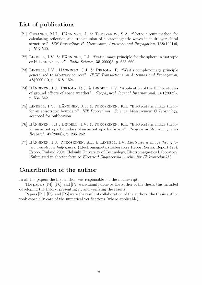
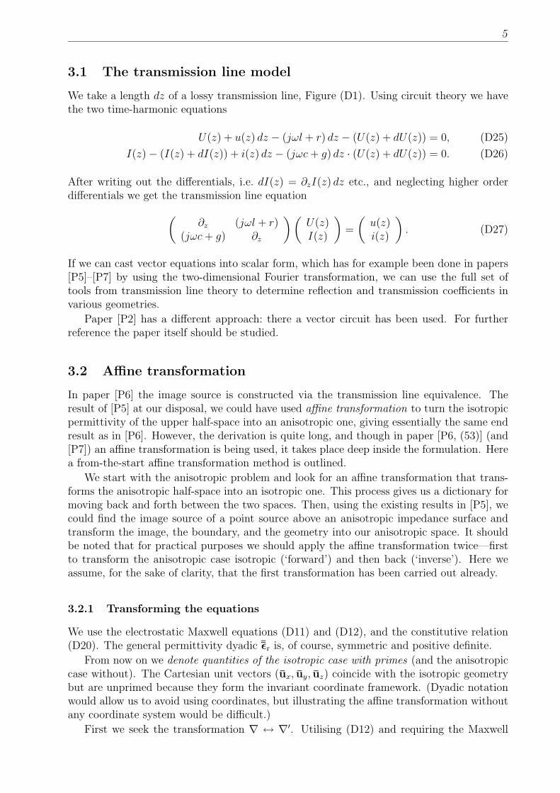
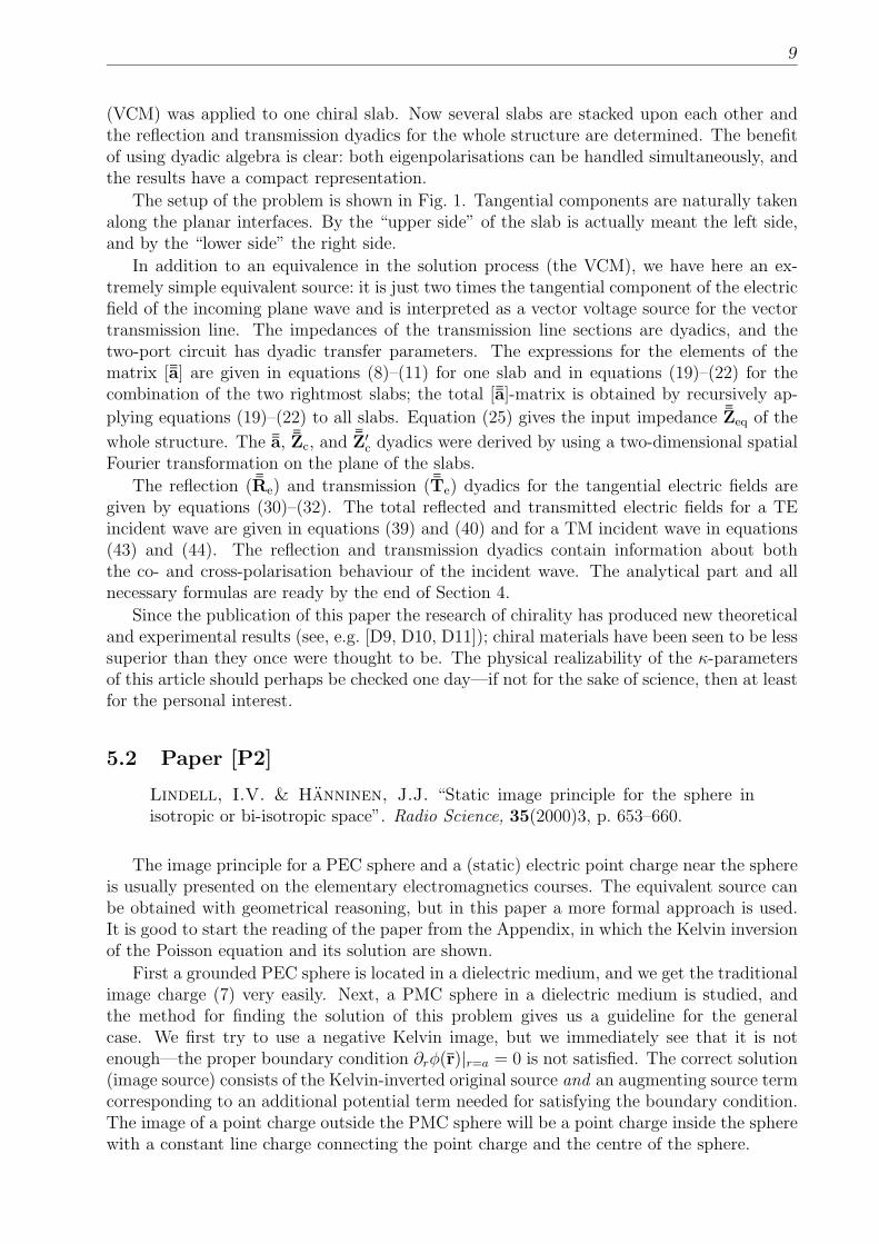
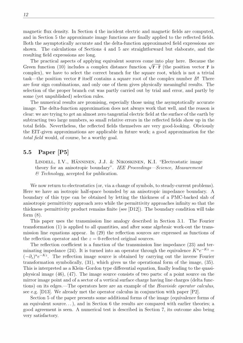
Figure D2: Equicharge contours in the x′′z-plane for the case discussed in Section 5.6. Thecircle denotes the shifted mirror image position.

5.6 Paper [P6]

Hanninen, J.J., Lindell, I.V. & Nikoskinen, K.I. “Electrostatic imagetheory for an anisotropic boundary of an anisotropic half-space”. Progress inElectromagnetics Research, 47(2004)-, p. 235–262.

The principal similarity of papers [P5]–[P7] makes it unnecessary to repeat all the detailsof the formulation. Of course, because [P6] and [P7] deal with an anisotropic half-space abovean anisotropic surface impedance or half-space, respectively, something new has to appear,and it is the two-dimensional dyadic ¯T. Constructing the transmission line equations ishelped by the existence of ¯T, inside which the details of the upper half-space medium areswept. Another significant innovation is the “shifting vector” a. In Section 4 the squareroot of ¯T is used twice to turn the anisotropic problem into an isotropic one (by an affinetransformation, actually), after which the known results of paper [P5] give us the solutionof this problem. The obtained image function is just a shifted, skewed, and slanted versionof the one in [P5].

The anisotropic permittivity dyadic ¯ǫr is the most general possible in electrostatics, i.e.it is symmetric and positive definite. As is evident from the paper, these two properties areheavily utilised in the solution process. The surface impedance dyadic ¯ζr possesses the samegenerality features.

14

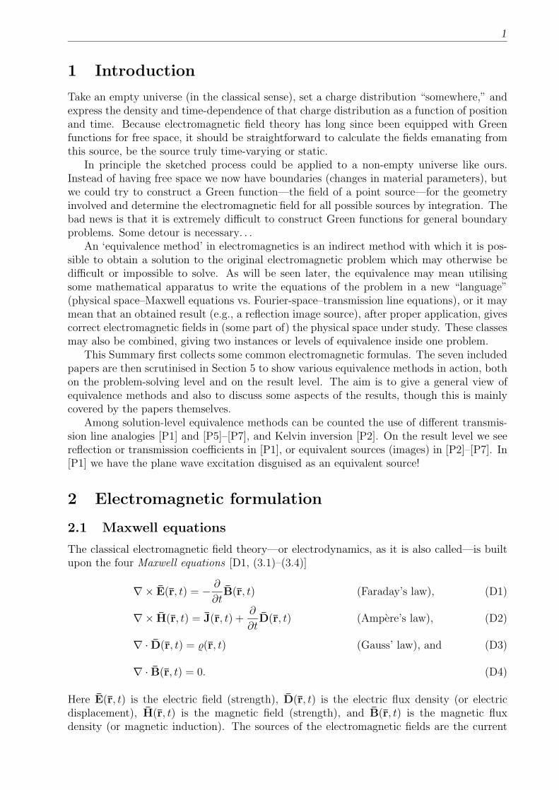
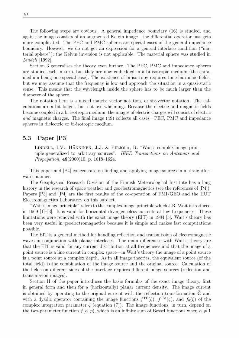
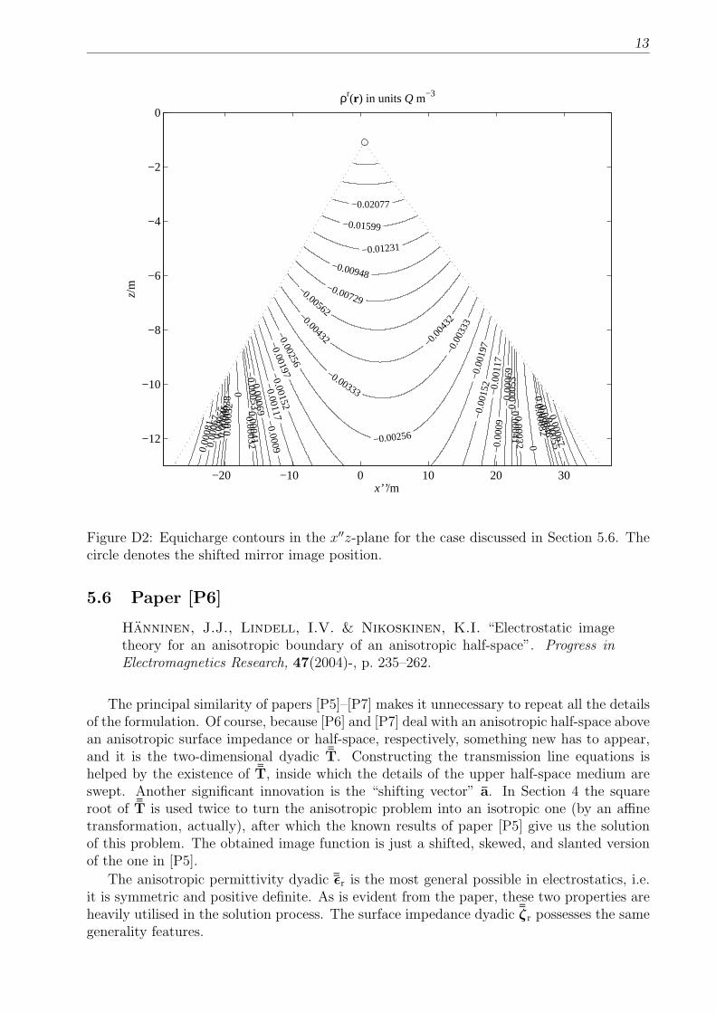
Figure D3: Charge distribution of the planar image source of Section 5.6. The true orienta-tion of the source is shown. Again the circle is in the location of the point source.

15

−4 −3 −2 −1 0 1 2 3 4−4

−3

−2

−1

0

1

2

3

4

y / m

z /

m

φr in units Q/(4πε0) m−1; x = 0 m

−0.084

−0.084

−0.079

−0.079

−0.074

−0.074

−0.

074

−0.069

−0.069

−0.

069

−0.064

−0.064

−0.

064

−0.059

−0.059

−0.

059

−0.054

−0.054

−0.054−0.049

−0.049

−0.049

−0.049

−0.044

−0.044

−0.044

−0.044 −0.039

−0.039

−0.0

39

−0.039

−0.034

−0.034

−0.034

−0.034

−0.029

−0.029−0.0

29

−0.029 −0.024

−0.024

−0.0

24

−0.024

−0.019

−0.019

−0.

019

−0.019

−0.014

−0.

014

−0.014

−0.014

−0.014 −0.009

−0.

009

−0.009

−0.009

−0.009

−0.004

−0.004

−0.004

−0.004

−0.004

0.001

0.00

1

0.001

0.001

0.001

0.00

10.006

0.006

0.0060.006

0.006

0.006

0.011

0.01

1

0.011

0.011

0.011

0.01

1

0.016

0.01

60.016

0.016

0.01

6 0.021

0.021

0.021

0.0210.

021

0.02

6

0.026

0.026

0.026

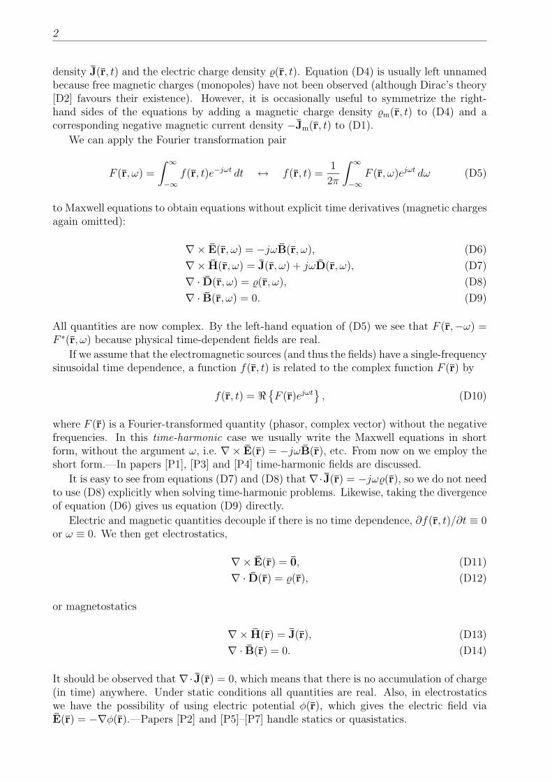
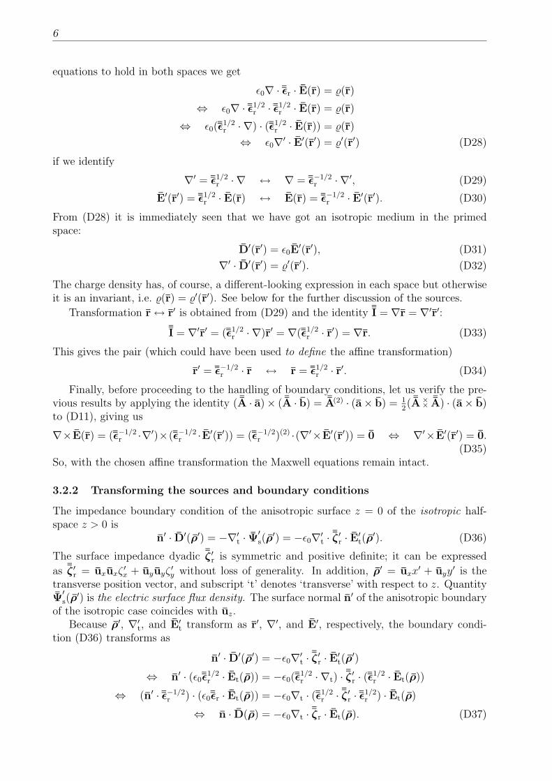
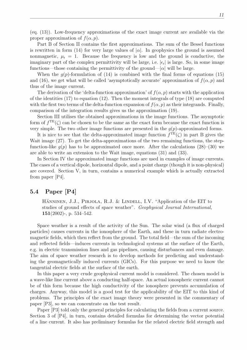
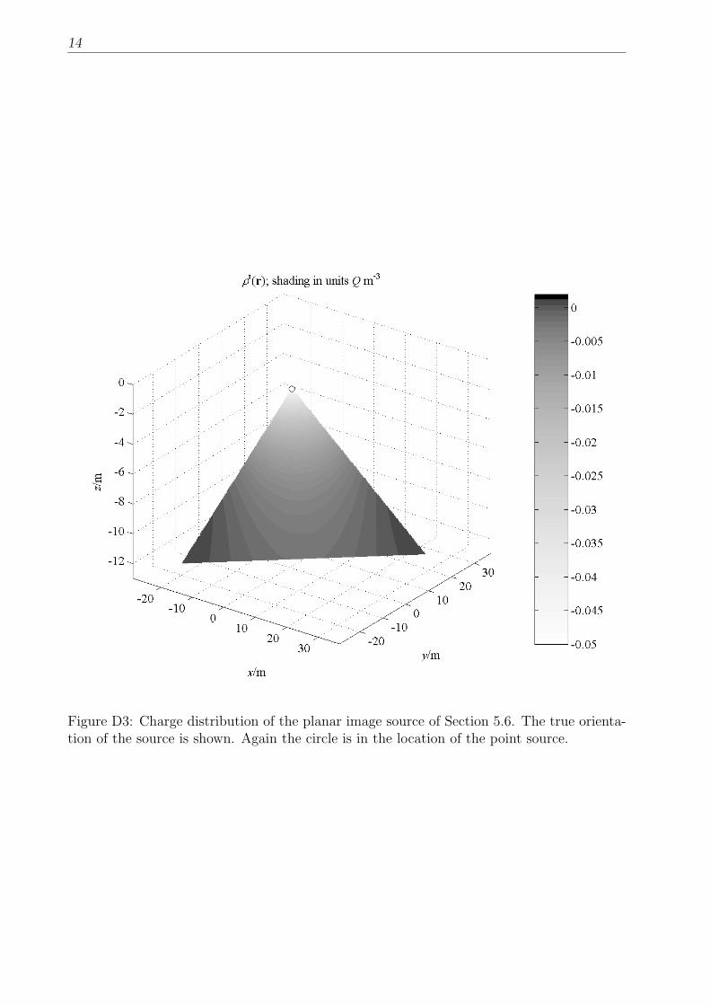
Figure D4: Equipotential contours in the x = 0 m plane for the reflection problem ofSection 5.6.

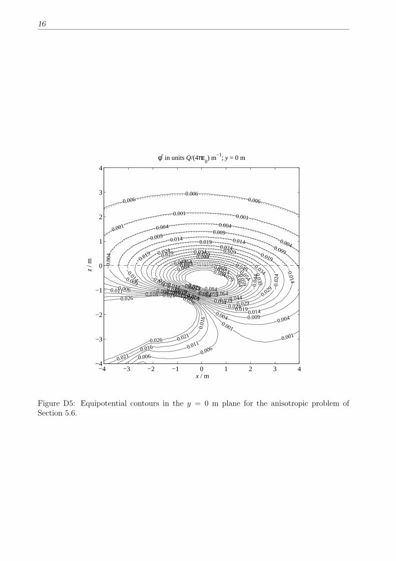
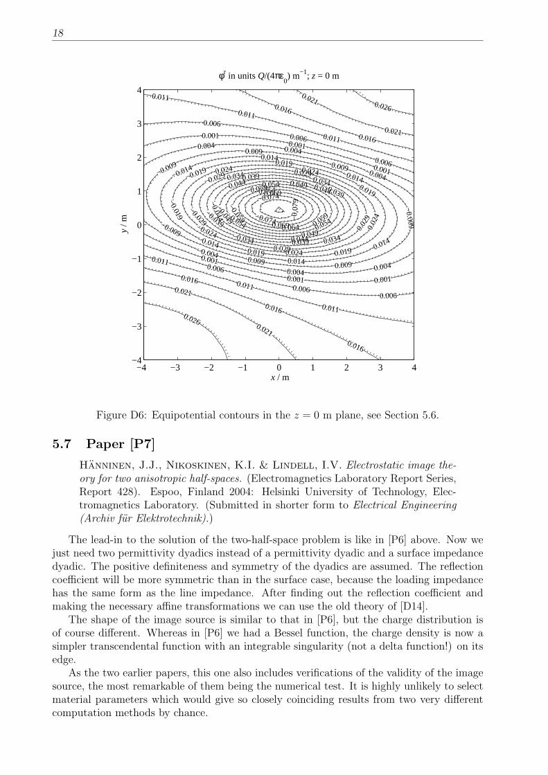
There are no potential figures in paper [P6], but that is mended here. We have chosenas the medium parameters—in close resemblance to [P7]—

¯ǫr = uxux8 + uyuy19/8 − (uyuz + uzuy)√

3/2 + uzuz2,

¯ζr = uxux32 + (uxuy + uyux)8√

3 + uyuy16, and z0 = 1.1 m, (D46)

giving us the computed parameters

a = −uy

√3/4, ζ ′

y = 2, and ζ ′′

d = 14. (D47)

The image charge distribution (excluding the edge charges) is presented in Figures (D2)and (D3). The normalised equipotential curves are shown in Figures (D4)–(D6). The agree-ment between the image theory results (solid lines) and inverse FFT comparison result(dotted lines) is clearly seen. The large curve-free voids in the lower half-space are dueto selecting the limited set of equipotential values from Figure (D6). The lower half-spacecurves are not physically valid in the sense of the original problem.

16

−4 −3 −2 −1 0 1 2 3 4−4

−3

−2

−1

0

1

2

3

4

x / m

z /

m

φr in units Q/(4πε0) m−1; y = 0 m

−0.084

−0.084

−0.079

−0.079−0.074

−0.074

−0.069

−0.069

−0.064

−0.064

−0.064

−0.059

−0.059

−0.059

−0.054

−0.054

−0.054

−0.049

−0.049 −0.049

−0.044

−0.044

−0.044−

0.04

4

−0.039

−0.039

−0.039

−0.039

−0.034

−0.034

−0.034

−0.034

−0.029

−0.029

−0.029 −0.029

−0.029

−0.024

−0.024

−0.024−0.024

−0.

024

−0.019

−0.019

−0.019

−0.019

−0.019

−0.014

−0.014

−0.014

−0.014 −0.014

−0.014

−0.009

−0.009

−0.009

−0.009−0.009

−0.009

−0.004−0.004

−0.004

−0.

004

−0.004 −0.004

−0.004

0.001

0.001

0.001

0.0010.001

0.001

0.0060.006

0.006

0.006

0.0060.006

0.006

0.0110.011

0.011

0.016

0.01

6

0.016

0.021

0.021

0.021

0.026

0.0260.026

Figure D5: Equipotential contours in the y = 0 m plane for the anisotropic problem ofSection 5.6.

17

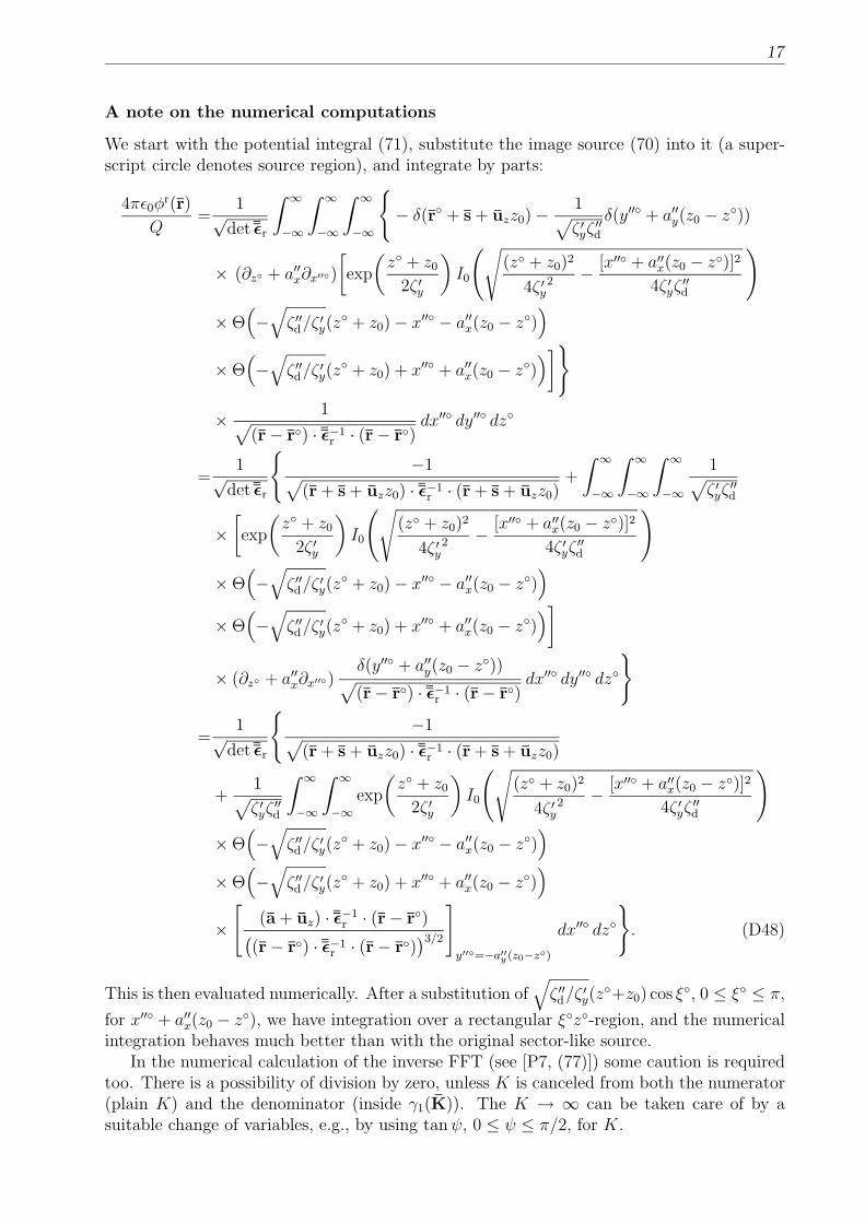
A note on the numerical computations

We start with the potential integral (71), substitute the image source (70) into it (a super-script circle denotes source region), and integrate by parts:

4πǫ0φr(r)

Q=

1√det¯ǫr

∫

∞

−∞

∫

∞

−∞

∫

∞

−∞

{

− δ(r◦ + s + uzz0) −1

√

ζ ′

yζ′′

d

δ(y′′◦ + a′′

y(z0 − z◦))

× (∂z◦ + a′′

x∂x′′◦)

[

exp

(

z◦ + z0

2ζ ′

y

)

I0

(√

(z◦ + z0)2

4ζ ′

y2 − [x′′◦ + a′′

x(z0 − z◦)]2

4ζ ′

yζ′′

d

)

× Θ(

−√

ζ ′′

d/ζ ′

y(z◦ + z0) − x′′◦ − a′′

x(z0 − z◦))

× Θ(

−√

ζ ′′

d/ζ ′

y(z◦ + z0) + x′′◦ + a′′

x(z0 − z◦))

]

}

× 1√

(r − r◦) · ¯ǫ−1r · (r − r◦)

dx′′◦ dy′′◦ dz◦

=1√

det¯ǫr

{

−1√

(r + s + uzz0) · ¯ǫ−1r · (r + s + uzz0)

+

∫

∞

−∞

∫

∞

−∞

∫

∞

−∞

1√

ζ ′

yζ′′

d

×[

exp

(

z◦ + z0

2ζ ′

y

)

I0

(√

(z◦ + z0)2

4ζ ′

y2 − [x′′◦ + a′′

x(z0 − z◦)]2

4ζ ′

yζ′′

d

)

× Θ(

−√

ζ ′′

d/ζ ′

y(z◦ + z0) − x′′◦ − a′′

x(z0 − z◦))

× Θ(

−√

ζ ′′

d/ζ ′

y(z◦ + z0) + x′′◦ + a′′

x(z0 − z◦))

]

× (∂z◦ + a′′

x∂x′′◦)δ(y′′◦ + a′′

y(z0 − z◦))√

(r − r◦) · ¯ǫ−1r · (r − r◦)

dx′′◦ dy′′◦ dz◦

}

=1√

det¯ǫr

{

−1√

(r + s + uzz0) · ¯ǫ−1r · (r + s + uzz0)

+1

√

ζ ′

yζ′′

d

∫

∞

−∞

∫

∞

−∞

exp

(

z◦ + z0

2ζ ′

y

)

I0

(√

(z◦ + z0)2

4ζ ′

y2 − [x′′◦ + a′′

x(z0 − z◦)]2

4ζ ′

yζ′′

d

)

× Θ(

−√

ζ ′′

d/ζ ′

y(z◦ + z0) − x′′◦ − a′′

x(z0 − z◦))

× Θ(

−√

ζ ′′

d/ζ ′

y(z◦ + z0) + x′′◦ + a′′

x(z0 − z◦))

×[

(a + uz) · ¯ǫ−1r · (r − r◦)

(

(r − r◦) · ¯ǫ−1r · (r − r◦)

)3/2

]

y′′◦=−a′′

y(z0−z◦)

dx′′◦ dz◦

}

. (D48)

This is then evaluated numerically. After a substitution of√

ζ ′′

d/ζ ′

y(z◦+z0) cos ξ◦, 0 ≤ ξ◦ ≤ π,

for x′′◦ + a′′

x(z0 − z◦), we have integration over a rectangular ξ◦z◦-region, and the numericalintegration behaves much better than with the original sector-like source.

In the numerical calculation of the inverse FFT (see [P7, (77)]) some caution is requiredtoo. There is a possibility of division by zero, unless K is canceled from both the numerator(plain K) and the denominator (inside γ1(K)). The K → ∞ can be taken care of by asuitable change of variables, e.g., by using tanψ, 0 ≤ ψ ≤ π/2, for K.

18

−4 −3 −2 −1 0 1 2 3 4−4

−3

−2

−1

0

1

2

3

4

x / m

y /

m

φr in units Q/(4πε0) m−1; z = 0 m

−0.

079

−0.074

−0.074

−0.069

−0.069−0.064

−0.064

−0.059

−0.059

−0.059

−0.054−0.054

−0.054

−0.049

−0.049

−0.049

−0.044

−0.044

−0.044−0.044

−0.039

−0.039

−0.039

−0.039

−0.034 −0.034

−0.034−0.034

−0.029

−0.029

−0.0

29

−0.029−0.029

−0.024

−0.024

−0.0

24

−0.024−0.024

−0.019

−0.019 −0.019

−0.019

−0.019

−0.019

−0.014

−0.014

−0.014

−0.014

−0.014

−0.014

−0.009

−0.009 −0.009

−0.009

−0.009

−0.009

−0.009

−0.004 −0.004

−0.004

−0.004

−0.004 −0.004

0.0010.001

0.001

0.001

0.001 0.001

0.006

0.006

0.006

0.006

0.0060.006

0.011

0.011

0.011

0.011

0.011

0.011

0.016

0.016

0.016

0.016

0.016

0.021

0.021

0.021

0.021

0.026

0.026

Figure D6: Equipotential contours in the z = 0 m plane, see Section 5.6.

5.7 Paper [P7]

Hanninen, J.J., Nikoskinen, K.I. & Lindell, I.V. Electrostatic image the-ory for two anisotropic half-spaces. (Electromagnetics Laboratory Report Series,Report 428). Espoo, Finland 2004: Helsinki University of Technology, Elec-tromagnetics Laboratory. (Submitted in shorter form to Electrical Engineering(Archiv fur Elektrotechnik).)

The lead-in to the solution of the two-half-space problem is like in [P6] above. Now wejust need two permittivity dyadics instead of a permittivity dyadic and a surface impedancedyadic. The positive definiteness and symmetry of the dyadics are assumed. The reflectioncoefficient will be more symmetric than in the surface case, because the loading impedancehas the same form as the line impedance. After finding out the reflection coefficient andmaking the necessary affine transformations we can use the old theory of [D14].

The shape of the image source is similar to that in [P6], but the charge distribution isof course different. Whereas in [P6] we had a Bessel function, the charge density is now asimpler transcendental function with an integrable singularity (not a delta function!) on itsedge.

As the two earlier papers, this one also includes verifications of the validity of the imagesource, the most remarkable of them being the numerical test. It is highly unlikely to selectmaterial parameters which would give so closely coinciding results from two very differentcomputation methods by chance.

19

6 Conclusion

Several equivalent sources and indirect solution methods in different geometries were presen-ted. Except of paper [P1] all equivalent sources were image sources. The most often usedsolution-level equivalence method was based on transmission line analogy.

Paper [P2] generalises the static image principle of the sphere to various spheres inisotropic or bi-isotropic media by using the Kelvin inversion. The history of image solutionsfor spherical geometries is also presented in the paper. The next step would be obtaininga good time-harmonic image theory for the sphere, but the task is very difficult or evenimpossible to carry out.

Paper [P3] contains the basic approximations suitable for geophysics and [P4] utilisesthem in a simple example. The planar geometry makes the use of the EIT possible, butgetting application-quality results needs further research. The next current model couldinclude a current line with vertical pulsating currents that prevent the accumulation ofcharges encountered in our example. There is a need for a fast calculation method of thefields at the surface of a layered earth. From the EIT point of view this is a true challengebecause the solution of the multilayered problem will be very complicated—the reflectionand transmission dyadics would be applied several times. There exists a solution for a slabin an otherwise homogeneous space [D15], but it is not applicable to geophysics as such.

As was mentioned with [P4], the selection of the branches of the square roots in the exactimage theory lacks well-established rules. One paper considers the subject [D16], but somequestions remain still unanswered. Especially, if we move to the multilayer problem, thechoice of the branches will become even more complicated.

Papers [P5]–[P7] give solutions, via the transmission-line model, for some canonical an-isotropic problems of electrostatics. These solutions, too, might find use in geophysics—especially if formulated for steady currents. The setting of [P7] could be studied further:there is room for a transmission image source, whose construction will probably be attemptedin the near future.

20

References

[D1] Lindell, I.V. Methods for Electromagnetic Field Analysis. 2nd ed. Piscataway, NJ1995: IEEE Press.

[D2] Dirac, P.A.M. “Quantised singularities in the electromagnetic field”. Proceedingsof the Royal Society of London, Series A, 133(1931)821, p. 60–72.

[D3] Landau, L.D., Lifshitz, E.M. & Pitaevskiı, L.P. Electrodynamics of Con-tinuous Media. (Landau and Lifshitz Course of Theoretical Physics; vol 8). 2nd ed.Oxford 1984: Pergamon Press.

[D4] Kong, J.A. Electromagnetic Wave Theory. Cambridge, MA 2000: EMW Publish-ing.

[D5] Lindell, I.V., Ermutlu, M.E., Nikoskinen, K.I. & Eloranta, E.H. “Staticimage principle for anisotropic conducting half-space problems: impedance bound-ary”. Geophysics, 59(1993)12, p. 1773–1778.

[D6] Nikoskinen, K.I. & Hanninen, J. “Kelvin’s inversion in wedge geometry”. In:Stuchly, M.A. & Shannon D.G., editors. Proceedings of the 2001 URSI Inter-national Symposium on Electromagnetic Theory; 2001 May 13–17; Victoria, Canada.2001: URSI. p. 119–121

[D7] Lindell, I.V. “Huygens’ principle in electromagnetics”. IEE Proceedings—Science,Measurement & Technology, 143(1996)2, p. 103–105.

[D8] Lindell, I.V. & Alanen, E. “Exact image theory for the Sommerfeld half-spaceproblem”. IEEE Transactions on Antennas and Propagation, 32(1984) no. 2, p. 126–133, no. 8, p. 841–847, no. 10, p. 1027–1032.

[D9] Ruotanen, L.H. & Hujanen, A. “Simple derivation of the constitutive paramet-ers of an isotropic chiral slab from wideband measurement data”. Microwave andOptical Technology Letters, 12(1996)1, p. 40–45.

[D10] Lindell, I.V., Sihvola, A.H., Puska, P. & Ruotanen, L.H. “Conditionsfor the parameter dyadics of lossless bianisotropic media”. Microwave and OpticalTechnology Letters, 8(1995)5, p. 268–272.

[D11] Ruotanen, L.H. & Hujanen, A. “Experimental verification of physical condi-tions restricting chiral material parameters”. Journal of Electromagnetic Waves andApplications, 11(1997)1, p. 21–35.

[D12] Lindell, I.V. & Nikoskinen, K.I. “Image method for electrostatic problemsinvolving planar anisotropic media based on transmission-line analogy”. Archiv furElektrotechnik, 77(1994)-, p. 251–257.

[D13] Lindell, I.V. “Heaviside operator calculus in electromagnetic image theory”.Journal of Electromagnetic Waves and Applications, 11(1997)-, p. 119–132.

[D14] Lindell, I.V., Nikoskinen, K.I. & Viljanen, A. “Electrostatic image methodfor the anisotropic half-space”. IEE Proceedings—Science, Measurement & Techno-logy, 144(1997)4, p. 156–162.

21

[D15] Lindell, I.V. “Exact image theory for the slab problem”. Journal of Electromag-netic Waves and Applications, 2(1988)2, p. 195–215.

[D16] Lindell, I.V. “On the integration of image sources in exact image method of fieldanalysis”. Journal of Electromagnetic Waves and Applications, 2(1988)7, p. 607–619.

421. I.V. Lindell, K.H. Wallén: Generalized Q-media and field decomposition in differential-form

approach, December 2003. 422. H. Wallén, A. Sihvola: Polarizability of conducting sphere-doublets using series of images,

January 2004. 423. A. Sihvola (editor): Electromagnetics Laboratory Annual Report 2003, February 2004. 424. J. Venermo, A. Sihvola: Electric polarizability of circular cylinder, February 2004. 425. A. Sihvola: Metamaterials and depolarization factors, February 2004. 426. T. Uusitupa: Studying electromagnetic wave-guiding and resonating devices, February 2004. 427. I.V. Lindell: Affine transformations and bi-anisotropic media in differential-form approach,

March 2004. 428. J.J. Hänninen, K.I. Nikoskinen, I.V. Lindell: Electrostatic image theory for two anisotropic

half-spaces, March 2004. 429. M. Norgren, J. Avelin, A. Sihvola: Depolarization dyadic for a cubic cavity: illustrations and

interpretation, March 2004. 430. K. Heiska: On the modeling of WCDMA system performance with propagation data, April 2004 431. J. Jylhä, A. Sihvola: Numerical modelling of random media using pseudorandom simulations,

April 2004. 432. S. Järvenpää, P. Ylä-Oijala: High order boundary element method for general acoustic

boundary value problems, April 2004. 433. P. Ylä-Oijala, M. Taskinen: General CFIE formulation for electromagnetic scattering by

composite metallic and dielectric objects. 434. Jari J. Hänninen: Solving electromagnetic boundary problems with equivalence methods, April

2004.

ISBN 951-22-7080-3

ISSN 1456-632X

Picaset Oy, Helsinki 2004