Received: 4 September 2018 Revised: 29 October 2018 Accepted: 15 November 2018

DOI: 10.1002/nla.2226

R E S E A R C H A R T I C L E

Solving bilinear tensor least squares problems andapplication to Hammerstein identification

Lars Eldén1 Salman Ahmadi-Asl2

1Department of Mathematics, LinköpingUniversity, Linköping, Sweden2Skolkovo Institute of Science andTechnology (Skoltech), Moscow, Russia

CorrespondenceLars Eldén, Department of Mathematics,Linköping University, 581 83 Linköping,Sweden.Email: lars.elden@liu.se

Funding informationMega Grant, Grant/Award Number:14.756.31.0001

AMS Subject Classification: 65F99, 65K10,15A69, 93E24

Summary

Bilinear tensor least squares problems occur in applications such as Hammer-stein system identification and social network analysis. A linearly constrainedproblem of medium size is considered, and nonlinear least squares solvers ofGauss–Newton-type are applied to numerically solve it. The problem is sepa-rable, and the variable projection method can be used. Perturbation theory ispresented and used to motivate the choice of constraint. Numerical experimentswith Hammerstein models and random tensors are performed, comparing thedifferent methods and showing that a variable projection method performs best.

KEYWORDS

bilinear regression, bilinear tensor least squares problem, Hammerstein identification,Gauss–Newton-type method, separable, variable projection

1 INTRODUCTION

Multidimensional arrays or tensors are generalizations of vectors and matrices. In this paper, we study the followinglinearly constrained bilinear tensor least squares (LBLS) problem:

minx,𝑦

|| · (x, 𝑦)2,3 − b||, eTi x = 1, (1)

where ∈ Rl×m×n is a tensor, and x ∈ Rm, 𝑦 ∈ Rn, b ∈ Rl, and ei is a canonical unit vector, for some i with 1 ≤ i ≤ m.Here, || · || is the Euclidean vector norm, and · (x, 𝑦)2,3 denotes tensor–vector–vector multiplication along modes2 and 3 (to be defined later). Throughout this paper, we assume that the LBLS problem (1) is overdetermined, that is,l > m + n − 1.

As we will demonstrate in Section 3, the bilinear problem is singular without the constraint. This is well known in theliterature on the Hammerstein model,1,2 and it is common to impose either a linear or a quadratic constraint on one ofthe unknown vectors and use an alternating algorithm. Typically, alternating algorithms converge slowly.3 We show thatby imposing the linear constraint as in (1), it is possible to apply standard, nonalternating methods for nonlinear leastsquares problems, with faster convergence to a stationary point. Thus, we describe the use of Gauss–Newton-type (G-N)methods (see, e.g., chapter 9 of the work of Björck4). Because the problem is separable, we can also use variable projection(VP) methods,3,5 where one of x and y is eliminated and an optimization problem in terms of the other is solved.

The main contribution of this paper is the development of perturbation theory for the LBLS problem and a study ofits consequences for algorithm design. We show that the convergence rate depends on the conditioning of the problem,which in turn depends on how the linear constraint is implemented, that is, which component of x or y is constrained tobe equal to 1. Thus, in the G-N methods, we choose the constraint that makes the Jacobian as well conditioned as possible.We also present perturbation theory, which shows that the conditioning of the solution parts x and y may be different.

Numer Linear Algebra Appl. 2018;e2226. wileyonlinelibrary.com/journal/nla © 2018 John Wiley & Sons, Ltd. 1 of 18https://doi.org/10.1002/nla.2226

2 of 18 ELDÉN AND AHMADI-ASL

In the VP methods, we constrain the part of the solution that is most well conditioned. A comparison of algorithms ismade, where a VP method comes out as winner.

The LBLS problem (1) with linear (or sometimes quadratic) constraint arises in the identification of a Hammersteinmodel; see, for example, the works of Bai et al.1 and Wang et al.,2 where the problem dimensions are usually quitesmall. There is a rather extensive literature on Hammerstein systems (see the references in the works of Wang et al.2 andDing et al.6), and the methods of this paper have been used before. For a very brief introduction to Hammerstein systemidentification, see Section 5.1.

The theory for bilinear systems of equations of the type · (x, 𝑦)2,3 = b is studied in the work of Johnson et al.,7 andsome applications are mentioned. Related bilinear and multilinear problems are used in statistics and chemometrics.8,9

Much larger problems occur in text analysis of news articles and social media10,11; here, the tensor is also sparse.The problem (1) can also be considered as a bilinear tensor regression problem. In the last couple of years, such problems

are becoming quite abundant in the literature; see, for example, two recent papers dealing with more general setups.9,12

However, most such papers are application oriented and do not deal with basic properties and algorithms (in fact, mostpropose alternating algorithms). In this paper, we are concerned with the simpler problem (1), we introduce perturbationanalysis, and we discuss and implement algorithms for problems of small and medium dimensions. This will be thestarting point for research concerning the more general problems.

For a comprehensive review of tensor decomposition and applications, see the work of Kolda et al.13

This paper is organized as follows. First, in Section 2, some necessary tensor concepts are defined. In Section 3, thenature of the singularity of the unconstrained bilinear least squares problem is discussed. Then, we show how to solve theLBLS problem using Gauss–Newton and VP methods. We present perturbation theory for the LBLS problem in Section 4.There, we also discuss how to implement the linear constraint numerically. Numerical experiments are reported inSection 5.

1.1 NotationWe let ||r|| be the Euclidean vector norm, and the subordinate matrix norm of A is denoted ||A||2. The Frobenius normof a tensor is written ||||. The identity matrix of dimension n is denoted In, and its column vectors, the canonical unitvectors, are denoted ei, for i = 1, 2,… ,n. We will use the notational convention

Rm ∋ x =

(1x

), x ∈ R

m−1, (2)

similar for x with subscripts.Let A ∈ Rm×n with m > n. The thin QR decomposition (see theorem 5.2.3 of the work of Golub et al.14) is A = QR,

where Q ∈ Rm×n has orthonormal columns, and R ∈ Rn×n is upper triangular.The term tensor is used to denote multidimensional arrays, denoted by calligraphic letters, ∈ Rl×m×n. In this paper,

we restrict ourselves to three-dimensional tensors. For matrices, we use Roman capital letters, and for vectors, Romansmall letters.

2 TENSOR CONCEPTS

To denote elements in a tensor, we use two equivalent notations, (i, 𝑗, k) = ai𝑗k. A fiber is a subtensor, where all indicesexcept one are fixed, for example, (i, ∶, k). A fiber can be identified with a vector.

Multiplication of a tensor by a matrix U ∈ Rp×l is defined

Rp×m×n ∋ = (U)1 ·, bi𝑗k =

l∑𝜇=1

ui𝜇a𝜇𝑗k.

This is equivalent to multiplying all mode-1 fibers in by the matrix U. Multiplication in the other modes is analogous.Simultaneous multiplication in all three modes is denoted (U,V ,W) ·. A special notation is used for multiplication by

ELDÉN AND AHMADI-ASL 3 of 18

a transposed matrix; let U ∈ Rl×p:

Rp×m×n ∋ = (UT)1 · =∶ · (U), bi𝑗k =

l∑𝜇=1

a𝜇𝑗ku𝜇i.

Multiplication of a tensor by a vector is analogous; for instance, assuming conforming dimensions,

· (x, 𝑦)2,3 ∈ Rl×1×1.

We will also let · (x, 𝑦)2,3 ∈ Rl. The notation · (x, ·)2,3 will be used for a linear operator,

· (x, ·)2,3 ∶ Rn ∋ 𝑦 → · (x, 𝑦)2,3 ∈ R

l. (3)

We will also use the same notation for the matrix in Rl×n of the operator. The operator and matrix · (·, 𝑦)2,3 are definedanalogously.

Matrices are assumed to have rows and columns, and vectors are usually column vectors. However, the different modesof a tensor are not associated with rows or columns, et cetera, until we explicitly do so. This means that · (u, v)2,3 ∈ Rl×1×1

is neither a column vector or a row vector, until we do such an association explicitly.

3 ALGORITHMS FOR SOLVING THE LBLS PROBLEM

Let x and y be arbitrary and choose 𝛼 ≠ 0. Clearly, · (x, 𝑦)2,3 = · (𝛼x, 1∕𝛼𝑦)2,3. Thus, the residual

r(x, 𝑦) = · (x, 𝑦)2,3 − b (4)

is constant along the curve (𝛼x, 1∕𝛼 y) in Rm×Rn. It follows that the Jacobian is rank deficient in the direction of the curveand the problem (1) without constraint is indeterminate. This indeterminacy is well known; see, for example, the worksof Bai et al.1 and Wang et al.2 In order to remove it, we impose a linear constraint that prevents the solution from movingalong the curve. In our description of methods, we will, for simplicity of presentation and without loss of generality, letthe constraint be eT

1 x = 1. Thus, we consider the constrained minimization problem (1) with i = 1. We will discuss inSection 4.3 how to implement the constraint in a numerically sound way. Alternative ways of handling the indeterminacyare described in the works of Bai et al.,1 Wang et al.,2 and Ding et al.6

In this section, we describe Gauss–Newton and VP methods for solving the LBLS problem.

3.1 The gradient and HessianWith the residual defined in (4), let the objective function be

𝑓 (x, 𝑦) = 12

r(x, 𝑦)Tr(x, 𝑦),

where r(x, y) = (r1(x, y), r2(x, y),… , rl(x, y))T. Then, the gradient is4(p340)

∇𝑓 (x, 𝑦) = J(x, 𝑦)Tr(x, 𝑦),

where J(x, y) is the Jacobian of r(x, y). From the bilinearity, we get the identity

r(x + s, 𝑦 + t) − r(x, 𝑦) = · (s, 𝑦)2,3 + · (x, t)2,3 + · (s, t)2,3

=( · (·, 𝑦)2,3 · (x, ·)2,3

)( st

)+ · (s, t)2,3,

and it is seen thatJ(x, 𝑦) = (Jx J𝑦) ∈ R

l×(m+n),

where Jx and Jy are matrices identified with the operators · (·, 𝑦)2,3 and · (x, ·)2,3, respectively.The rank deficiency of J is now obvious because

J(

x−𝑦

)= 0.

4 of 18 ELDÉN AND AHMADI-ASL

Clearly, J is rank deficient everywhere.The residual for the constrained problem is r(x, 𝑦) = r(x, 𝑦), with x given by (2). The Jacobian of r is

J(x, 𝑦) = (Jx J𝑦) ∈ Rl×(m+n−1), (5)

where the matrix Jx is defined to be Jx with the first column deleted.The gradient for the constrained problem can be written

∇𝑓 = JTr = J · (r)1 = ( · (r, ·, 𝑦) · (r, x, ·)).

The Hessian becomes

H = J · (J)1 +

( 𝜕

𝜕x𝜕

𝜕𝑦

)( · (r, ·, 𝑦) · (r, x, ·)

)= J · (J)1 +

(0 ( · (r)1) · (·)3

( · (r)1) · (·)2 0

),

which can be identified with

H = JT J +(

0 Ar��T

r 0

), (6)

where Ar is the matrix R(m−1)×n ∋ Ar = · (r)1 and = (∶, 2 ∶ m, ∶).

3.2 Gauss–Newton methodsGauss–Newton methods are iterative schemes to solve nonlinear least-squares problems; see, for example, chapter 9 ofthe work of Björck.4 Let (xk; yk) be an approximation of the solution. In the Gauss–Newton method for solving (1) with theconstraint eT

1 x = 1, the following linear least squares problem is solved at iteration k:

minp

12||Jp + rk||2, p =

(pxp𝑦

), (7)

where rk = r(xk, 𝑦k), J = J(xk, 𝑦k), and px ∈ Rm−1. The new iterate is(xk+1𝑦k+1

)=(

xk𝑦k

)+ pk, pk =

(0p

)=

( 0pxp𝑦

).

The QR or SVD decompositions can be used to solve the linear least squares problem (7). The Gauss–Newton method hasfast local convergence rate for problems with small residuals and nonlinear structure; see the work of Björck.4(p343)

The damped Gauss–Newton method4(p343) is designed to be more robust than the Gauss–Newton method; at iteration k,after finding the Gauss–Newton correction pk = (px, py), a line search is performed along pk, by finding an approximatesolution 𝛼k of the following one-dimensional minimization problem:

min𝛼≥0

|| · (xk + 𝛼px, 𝑦k + 𝛼p𝑦)2,3 − b||2,and the new iterate is (

xk+1𝑦k+1

)=(

xk𝑦k

)+ 𝛼kpk.

By straightforward calculation, we have

· (xk + 𝛼px, 𝑦k + 𝛼p𝑦)2,3 − b = · (xk, 𝑦k)2,3 + 𝛼( · (xk, p𝑦)2,3 + · (px, 𝑦k)2,3

)− b + 𝛼2 · (px, p𝑦)2,3,

and

g(𝛼) = || · (xk + 𝛼px, 𝑦k + 𝛼p𝑦)2,3 − b||2= ||𝛽||2𝛼4 + (2𝛽T𝛾)𝛼3 + (𝛾T𝛾 + 2rT𝛽)𝛼2 + (2𝛾Tr)𝛼 + ||r||2,

wherer = · (xk, 𝑦k)2,3 − b, 𝛾 = · (xk, p𝑦)2,3 + · (px, 𝑦k)2,3, 𝛽 = · (px, p𝑦)2,3.

ELDÉN AND AHMADI-ASL 5 of 18

The function g(𝛼) is a fourth-degree polynomial in 𝛼, so after the coefficients of the polynomial are computed, a linesearch is very cheap, as we avoid computing extra tensor–vector multiplications. The actual line search is performedusing MATLAB's one-dimensional function minimizer fminbd.

3.3 The VP methodAs the LBLS problem (1) is bilinear, that is, linear in each of x and y separately, it is a separable nonlinear least squaresproblem in the sense of the work of Golub et al.,5 which can be solved by the VP method. For notational convenience, werewrite the residual in (1) as ||𝜙x(𝑦) − b||,where, for fixed x satisfying (2), 𝜙x(·) = · (x, ·)2,3. To formulate the Golub–Pereyra scheme from the work of Golub et al.5for our separable problem, we use the Moore–Penrose pseudoinverse of 𝜙x. For fixed x, the solution of min𝑦 ||𝜙x(𝑦) − b||,is given by 𝑦 = 𝜙+

x b. Therefore, (1) is equivalent to

mineT

1 x=1||(Il − P𝜙x )b||2, 𝑦 = 𝜙+

x b, (8)

where P𝜙x = 𝜙x𝜙+x , is an orthogonal projector.

The VP method of Golub et al.5 is essentially the Gauss–Newton method applied to the nonlinear least squaresproblem (8). Thus, we shall compute the gradient with respect to x of

𝑓 (x) = 12||(Il − P𝜙x )b||2.

As in Section 3.1, we need to compute the Jacobian of r(x) = (Il − P𝜙x )b. We have

J(x) = −D(P𝜙x )b, (9)

where D(P𝜙x ) is the Fréchet derivative with respect to x of the orthogonal projector P𝜙x . Kaufman15 proposed an approxi-mation, which is demonstrated to be more efficient than the exact formula (see lemma 4.1 of the work of Golub et al.5).In the notation of Kaufman,15

J = P⟂𝜙x

D(𝜙x)𝜙+x b, (10)

where P⟂𝜙x

= Il − 𝜙x𝜙+x . Note that J is a matrix/operator*. Clearly, as 𝜙x(·) = · (x, ·)2,3, and because we differentiate with

respect to x, the Fréchet derivative is · (·)3, where = (∶, 2 ∶ m, ∶). Thus, because 𝜙+x b ∈ Rn, we can write

D(𝜙x)𝜙+x b = · (𝜙+

x b)3 ∈ Rl×(m−1).

Now recall that 𝜙x = Jy. Let the thin QR decomposition of 𝜙x ∈ Rl×n be

𝜙x = J𝑦 = Q𝑦R𝑦, Q𝑦 ∈ Rl×n, R𝑦 ∈ R

n×n.

Then, assuming that 𝜙x has full column rank, 𝜙+x = R−1

𝑦 QT𝑦 , and P⟂

𝜙x= I − Q𝑦QT

𝑦 . Now, (10) becomes

J ∶ Rm−1 → R

l,

J(·) =(

P⟂𝜙x

D(𝜙x)𝜙+x b

)(·) =

(Il − Q𝑦QT

𝑦

)1 ·([

·(·,R−1

𝑦 QT𝑦 b

)2,3

]). (11)

This formula makes perfect sense: We eliminate the variable y and project so that the range of J becomes orthogonal tothat of Jy. Thus, in the approximate Gauss–Newton method for (8), we compute the correction px for x, by solving theleast squares problem

minpx

||Jpx + r||.We will refer to this method as VPx.

By analogous derivations, one can formulate the VP method for the case when the constraint is still imposed on x, butx is eliminated and a minimization problem for y is solved. Here, we write||𝜓𝑦(x) − b(𝑦)||, 𝜓𝑦(·) = · (·, 𝑦)2,3, b(𝑦) = b −1 · (𝑦)3,

*The slight confusion in (10) is due to the numerical linear algebra conventions for matrix–vector multiplication. The formula is clarified in (11).

6 of 18 ELDÉN AND AHMADI-ASL

where = (∶, 2 ∶ m, ∶) and1 = (∶, 1, ∶). Let A1 be the matrix identified with1. The approximate Jacobian becomes

−(

Il − 𝜓𝑦𝜓+𝑦

)1 ·[(

·(𝜓+𝑦 b(𝑦), ·

)2,3 + A1

)].

This method will be referred to as VPy.

3.4 Newton's methodDue to the bilinear nature of the problem, the cost for an iteration with Newton's method is of the same order of magnitudeas for the other methods; see Section 3.6. A Newton step amounts to solving Hp = −JTr, where H and p are given by (6)and (7), respectively.

As Newton's method is sensitive to the initial approximation, we cannot expect it to converge properly if used as astand-alone method. We will use it in combination with VPx for problems with slower convergence.

3.5 Alternating least squares algorithmAlternating algorithms are often used for solving the bilinear problem.1,2 First, an initial approximation for y is inserted,and then, the linear least squares problem for x is solved. Then, the newly computed x is inserted and one solves for y.After each such iteration, the solution is normalized, for example, by putting one component of x equal to 1, and rescalingx and y accordingly. Typically, alternating algorithms converge slowly and, in general, they are not guaranteed to convergeto a local minimizer.3,16 We will see below that the convergence rate depends strongly on the conditioning of the problem.

We will refer to the alternating method as ALS. We will also perform a few ALS iterations as a starting method for theG-N and VP methods.

3.6 Computational workHere and in Section 5, we will compare the following methods:

• Gauss–Newton (G-N),• Damped Gauss–Newton (DG-N),• variable projection (VPx and VPy),• variable projection followed by Newton (VPxN), and• alternating iterations (ALS).

We first emphasize that, for the problems that occur, for example, in Hammerstein identification, the dimensions areso small that measuring the computational work in terms of operation counts is irrelevant; only the rate of convergenceand accuracy matter.

On the other hand, because large and sparse tensors occur in some applications,10,11 it is of interest to discuss how largeproblems with dense tensors can be solved by the methods of this paper.

Clearly, for large and dense problems, memory may become a concern. For instance, a tensor of dimensions 1000 ×500 × 500 requires about 2 GB of memory, which may be large on some computers.

The operations with highest operation counts are tensor–vector multiplication (ttv in the TensorToolbox17), QR factor-ization, and matrix multiplication, which all have third-order complexity, that is, O(lmn), essentially. However, becauseQR and matrix multiplication are performed with highly optimized code, and because ttv for large dense tensors is prob-ably dominated by data movement, ttv can be expected to be slower than QR and matrix multiplication. We performeda timing experiment in MATLAB with a 800 × 300 × 300 tensor, and here, the times for tensor–vector multiplication inthe first and second modes were 4–5 times longer (0.5 s) than for multiplication in the third mode. In connection withthe same tensor, a QR decomposition of a 800 × 600 matrix (such as in G-N) required 0.03 s, approximately.

Thus, we can get a rough comparison between the methods by counting how many ttv's, QR decompositions, andmatrix multiplications are performed per iteration. The residual r is needed for the gradient computation; here, one canreuse the Jacobian so that no extra ttv is needed. In VPx, VPy, and ALS, the QR decompositions are for the blocks of theJacobians. Therefore, to make it a fair comparison, we have counted each such computation as one half QR. We give thenumbers in Table 1, which shows that all methods require roughly the same work per iteration.

ELDÉN AND AHMADI-ASL 7 of 18

TABLE 1 The number of operations per iteration

G-N DG-N VPx VPy Newton ALS

ttv 2 3 3 3 3 3QR 1 1 1.5 1.5 1 1Matrix mult. 1 1

From the above arguments and Table 1, we see that it makes sense to compare the efficiency of all the methods bycounting the number of iterations for convergence.

3.7 Convergence rate IIt is shown in the work of Ruhe et al.3 that all the methods mentioned, except ALS, may have asymptotic superlinearconvergence (of course, Newton's method has quadratic convergence). The convergence rates of the G-N and VP methodsdepend in a nontrivial way on the Hessian matrix for the iterations, but the conclusion of Ruhe et al.3 is that they stillhave essentially the same convergence rate. We will see this in the numerical experiments.

For problems with residual r close to zero, that is, where the data fit the model well, and the noise level of the data issmall, all methods, except ALS, exhibit almost quadratic convergence. This is because the second term in the Hessian (6)becomes insignificant as the iterations proceed, and the G-N and VP methods approach Newton's method. For problemswith larger residual, we get linear convergence.3(p320)

We come back to convergence rate in Section 4.2.

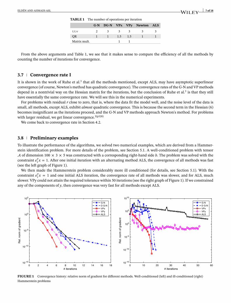
3.8 Preliminary examplesTo illustrate the performance of the algorithms, we solved two numerical examples, which are derived from a Hammer-stein identification problem. For more details of the problem, see Section 5.1. A well-conditioned problem with tensor of dimension 100 × 3 × 5 was constructed with a corresponding right-hand side b. The problem was solved with theconstraint eT

1 x = 1. After one initial iteration with an alternating method ALS, the convergence of all methods was fast(see the left graph of Figure 1).

We then made the Hammerstein problem considerably more ill conditioned (for details, see Section 5.1). With theconstraint eT

1 x = 1 and one initial ALS iteration, the convergence rate of all methods was slower, and for ALS, muchslower. VPy could not attain the required tolerance within 50 iterations (see the right graph of Figure 1). If we constrainedany of the components of y, then convergence was very fast for all methods except ALS.

0 2 4 6 8 10 12 14 16 18

# iterations

10

10

10

10

10

Rel

. nor

m o

f gra

dien

t

0 10 20 30 40 50 60

# iterations

10

10

10

10

10

10

Rel

. nor

m o

f gra

dien

t

FIGURE 1 Convergence history: relative norm of gradient for different methods. Well-conditioned (left) and ill-conditioned (right)Hammerstein problems

8 of 18 ELDÉN AND AHMADI-ASL

Clearly, the convergence properties depend on the conditioning of the problem and on how the linear constraint ischosen. These two examples demonstrate that an understanding of the conditioning of the LBLS problem is needed.

4 PERTURBATION THEORY

Consider the first-order condition for the linearly constrained BLS problem,

JTr(x, 𝑦) = 0,

where J is defined in (5), and (x, y) is a stationary point. Add a small perturbation to the tensor and the right-hand side, = + 𝛿 and b = b + 𝛿b, where

||𝛿|| ≤ 𝜖, ||𝛿b|| ≤ 𝜖. (12)

Further, assume that the perturbation of is so small that the perturbed Jacobian JT has full column rank, and theperturbed Hessian is positive definite. Denote the perturbed solution

x + 𝛿x =(

1x

)+(

0𝛿x

), 𝑦 + 𝛿𝑦, r + 𝛿r. (13)

A straightforward calculation (see Appendix A) shows that the first-order condition, after omitting terms that are (𝜖2),gives the following equation for the perturbation of the solution:

⎛⎜⎜⎝−I Jx J𝑦JT

x 0 Ar

JT𝑦 ��T

r 0

⎞⎟⎟⎠(𝛿r𝛿x𝛿𝑦

)=

(𝛿b − 𝛿 · (x, 𝑦)2,3−𝛿 · (r, 𝑦)1,3−𝛿 · (r, x)1,2

), (14)

where Ar is identified with · (r)1, and 𝛿 · (r, 𝑦)1,3 ∈ Rm−1 and 𝛿 · (r, x)1,2 ∈ Rn are treated as column vectors. Thematrix in (14) is the Hessian when r has been included in the problem formulation.

In order to express the solution conveniently, we rewrite (14) as(−I JJT Tr

)(𝛿r𝛿z

)=(𝛿b − 𝛿 · (x, 𝑦)2,3

𝛿(r, x, 𝑦)

), (15)

where

Tr =(

0 Ar��T

r 0

), 𝛿z =

(𝛿x𝛿𝑦

), 𝛿(r, x, 𝑦) =

(−𝛿 · (r, 𝑦)1,3−𝛿 · (r, x)1,2

). (16)

The solution is (𝛿r𝛿z

)=(−I + JH−1JT JH−1

H−1JT H−1

)(𝛿b − 𝛿 · (x, 𝑦)2,3

𝛿(r, x, 𝑦)

), (17)

where H = JT J + Tr is the Hessian (6).We can now estimate the perturbations ||𝛿r|| and ||𝛿z||.Theorem 1. Consider the bilinear least squares problem with linear equality constraint (1) with full rank Jacobian Jand positive definite Hessian H. Let + 𝛿 and b + 𝛿b be perturbed data and assume that 𝛿 is so small that theperturbed Jacobian has full rank, and the perturbed Hessian is positive definite. Let (x, y) be a stationary point, and denotethe perturbed solution as in (13). Then, if second-order terms are neglected, we can estimate from (17)

||𝛿r|| ⪅ (1 +

𝜎2max(J)

𝜆min(H)

)(||𝛿b|| + ||𝛿 · (x, 𝑦)2,3||) + 𝜎max(J)||r|| ||𝛿||𝜆min(H)

‖‖‖‖‖(

x𝑦

)‖‖‖‖‖ , (18)

‖‖‖‖‖(𝛿x𝛿𝑦

)‖‖‖‖‖ ⪅ 𝜎max(J)𝜆min(H)

(||𝛿b|| + ||𝛿 · (x, 𝑦)2,3||) + ||r|| ||𝛿||𝜆min(H)

‖‖‖‖‖(

x𝑦

)‖‖‖‖‖ , (19)

where 𝜆min(H) is the smallest eigenvalue of H and 𝜎max(J) is the largest singular value of J.

ELDÉN AND AHMADI-ASL 9 of 18

Proof. The results are proved by straightforward estimation of the terms in (17), using ||H−1||2 ≤ 1∕𝜆min(H) and||J||||2 ≤ 𝜎max(J). The last term in both right-hand sides follows from

‖‖‖𝛿(r, x, 𝑦)‖‖‖2=‖‖‖‖‖(𝛿 · (r, 𝑦)1,3𝛿 · (r, x)1,2

)‖‖‖‖‖2

≤(||𝛿||2 ||𝑦||2 + ||𝛿||2 ||x||2) ||r||2,

using ||𝛿|| ≤ ||𝛿||.The estimates (18) and (19) are fundamental in the sense that they are based on the geometry of the problem at the

stationary point (see section 9.1.2 of the work of Björck4 and see also the work of Wedin18). However, the eigenvalues of Hdepend on the residual and that dependence is not visible in the estimates. Therefore, in Theorem 2, we derive alternativeestimates that are valid for small residuals. First, we give two lemmas.

Lemma 1. Let Tr be defined by (16).Then,

||Tr||2 ≤ |||| ||r||. (20)

Proof. Because the eigenvalues of the symmetric matrix Tr are plus/minus the singular values of Ar, we have ||Tr||2 =||Ar||2. Let A(1) be the mode-1 matricization of , that is, it is the matrix whose columns are all the mode-1 vectorsof . Then, ||Ar||2 = || · (r)1||2 = ||rTA(1)||2 ≤ ||r|| ||A(1)||2 ≤ ||r|| ||A(1)|| = ||r|| |||| ≤ ||r|| ||||,where we have used the inequality ||A||2 ≤ ||A||.Lemma 2. Let J = QR be the thin QR decomposition, and let 𝜎min(J) =∶ 𝜎min > 0 be the smallest singular value of J(and R). Assume that, at a stationary point, |||| ||r||

𝜎2min

= 𝜂 < 1, (21)

holds. Then,

||H−1||2 ≤1𝜎2

min

11 − 𝜂

, (22)

||JH−1||2 ≤1𝜎min

11 − 𝜂

, (23)

||JH−1JT||2 ≤1

1 − 𝜂. (24)

Proof. Using the QR decomposition, we have

H−1 =(

RTR + Tr)−1 = R−1(I + R−TTrR−1)−1R−T ,

and ||H−1||2 ≤ ||R−1||22 ||(I + R−TTrR−1)−1||2.By Lemma 1 and assumption (21), we have ‖‖R−TTrR−1‖‖2 ≤ 𝜂 < 1.

For any matrix X, which satisfies ||X||2 < 1, we can estimate ||(I + X)−1||2 < 1∕(1 − ||X||2). Therefore, we get

||H−1||2 ≤1𝜎2

min

11 − 𝜂

.

The proofs of the other two inequalities are analogous.

It is seen from section 9.1.2 of the work of Björck4 that (21) is a sufficient condition for the Hessian to be positivedefinite and, thus, for the stationary point to be a local minimum. In section 9.1.2 of the work of Björck,4 a slightly weakercondition is used; however, using (21), we can see in the following theorem the likeness to the perturbation theory for thelinear least squares problem.

10 of 18 ELDÉN AND AHMADI-ASL

Theorem 2. Let the assumptions of Theorem 1 hold, and further assume that (21) is satisfied. Then, if second-orderterms are neglected, we can estimate from (17),

||𝛿r|| ⪅ 11 − 𝜂

((2 − 𝜂)(||𝛿b|| + ||𝛿 · (x, 𝑦)2,3||) + ||r|| ||𝛿||

𝜎min

‖‖‖‖‖(

x𝑦

)‖‖‖‖‖), (25)

‖‖‖‖‖(𝛿x𝛿𝑦

)‖‖‖‖‖ ⪅ 11 − 𝜂

(1𝜎min

(||𝛿b|| + ||𝛿 · (x, 𝑦)2,3||) + ||r|| ||𝛿||𝜎2

min

‖‖‖‖‖(

x𝑦

)‖‖‖‖‖). (26)

Proof. The results are proved by straightforward estimation of the terms in (17), using Lemma 2.

The estimates (25)–(26) have (not surprisingly) the same structure as the corresponding estimates for the linear leastsquares problem; see, for example, theorem 2.2.6 of the work of Björck.4 For instance, if r = 0, then the conditioning ofthe solution x and y together depends essentially on the condition number of the Jacobian. However, if r ≠ 0, there isalso a dependence on the square of the condition number of the Jacobian in the form ||r||∕𝜎2

min.The second estimate (19) has the disadvantage that 𝛿x and 𝛿y are lumped together. Due to the bilinear and separable

nature of the problem, one would like to have separate estimates for these perturbations. We will now derive such a resultfor the case r = 0.

4.1 Estimates of ||𝜹x || and ||𝜹y || in the case r= 0Assuming that the problem is consistent, r = 0, we derive explicit expressions for the perturbations 𝛿x and 𝛿y. We furtherassume that J has full column rank. Using the partitioned Jacobian (5), we can write the second equation of (17) as

S(𝛿x𝛿𝑦

)=(

JTx Jx JT

x J𝑦JT𝑦 Jx JT

𝑦 J𝑦

)(𝛿x𝛿𝑦

)=(

JTx

JT𝑦

)c, (27)

where c = 𝛿b − 𝛿 · (x, 𝑦)2,3. Let the thin QR decompositions of the blocks of J be

Jx = QxRx, Qx ∈ Rl×(m−1), Rx ∈ R

(m−1)×(m−1), (28)

J𝑦 = Q𝑦R𝑦, Q𝑦 ∈ Rl×n, R𝑦 ∈ R

n×n, (29)where the columns of Qx and Qy are orthonormal, and Rx and Ry are upper triangular and nonsingular. Inserting the QRfactors in (27), we get (

RTx Rx RT

x QTx Q𝑦R𝑦

RT𝑦QT

𝑦QxRx RT𝑦R𝑦

)(𝛿x𝛿𝑦

)=(

RTx QT

x

RT𝑦QT

𝑦

)c. (30)

Defining (𝛿x𝛿𝑦

)=(

Rx 𝛿xR𝑦 𝛿𝑦

), (31)

E = QTx Q𝑦, and multiplying by the inverses of RT

x and RT𝑦 , (30) becomes(

I EET I

)(𝛿x𝛿𝑦

)=(

QTx

QT𝑦

)c.

It is easy to verify that (I E

ET I

)−1

=(

I + ES−1ET −ES−1

−S−1ET S−1

),

where S = I − ETE = QT𝑦 (I − QxQT

x )TQ𝑦. The nonsingularity of the Schur complement S follows from the fact that thematrix (

I EET I

)is positive definite. Therefore, we have

𝛿x =((I + ES−1ET)QT

x − ES−1QT𝑦

)c.

ELDÉN AND AHMADI-ASL 11 of 18

After rewriting this and using 𝛿x = Rx𝛿x, we get

𝛿x = R−1x QT

x Pxc, Px = I − Q𝑦

(QT𝑦

(I − QxQT

x)

Q𝑦

)−1QT𝑦

(I − QxQT

x). (32)

We recognize Px as an oblique projection; see, for example, the work of Hansen.19 Clearly, we have derived part of theMoore–Penrose pseuodoinverse of J.

Proposition 1. Assume that the matrix J = (Jx J𝑦) has full column rank and that the blocks have QR decompositions(28)–(29). Then, its Moore–Penrose pseudoinverse is equal to

J+ =(

J+x Px

J+𝑦 P𝑦

)=(

R−1x QT

x Px

R−1𝑦 QT

𝑦P𝑦

), (33)

where Px is defined in (32) and Py is symmetrically defined.

The proof is given in Appendix B.We now have the following theorem.

Theorem 3. Assume that, at the optimal point (x, y), the Jacobian J and the perturbed Jacobian have full column rankand that the residual satisfies r = 0. Let 𝜎min(Rx) > 0 and 𝜎min(R𝑦) > 0 be the smallest singular values of Rx and Ry,respectively. Then, to first order,

||𝛿x|| ⪅ ‖‖QTx Px‖‖

𝜎min(Rx)(||𝛿b|| + ||𝛿 · (x, 𝑦)2,3||), (34)

||𝛿𝑦|| ⪅ ‖‖QT𝑦P𝑦‖‖

𝜎min(R𝑦)(||𝛿b|| + ||𝛿 · (x, 𝑦)2,3||), (35)

where Px is defined in (32), and Py is symmetrically defined.

The theorem shows that, in this case, the conditioning of x and y depends on the condition number of Rx and Ry,respectively, and on the geometric properties of the range spaces of Jx and Jy.20 Note that the norm of an oblique projectionis usually larger than 1. If the range of Jx is orthogonal to that of Jy, that is, QT

x Q𝑦 = 0, then Px becomes an orthogonalprojection onto the null space of Jy, and QT

x Px = QTx , that is, the perturbations of 𝛿x and 𝛿y are completely independent.

If the residual is small and the problem is not too ill conditioned, that is, if|||| ||r||𝜎2

min

= 𝜂 ≪ 1,

is satisfied, then the estimates (34)–(35) hold approximately also in the case r ≠ 0. Therefore, it makes sense to basedecisions on the implementation of the linear constraint on the conditioning of Jx and Jy, separately.

4.2 Convergence rate IIFrom the work of Ramsin et al.21 and theorem 1 of the work of Wedin,18 one can prove that the convergence factor 𝜌of the Gauss–Newton method is bounded from above by the eigenvalue of the largest modulus of the curvature matrixK = −(J+)TTrJ+ at the stationary point†, where J+ is the Moore–Penrose pseudoinverse. Thus,

𝜌 ≤ maxi

|𝜆i(K)| =∶ ��. (36)

As J+ = R−1QT , the convergence rate depends on the conditioning of J. Moreover, we have an expression (33) for thepseudoinverse, which, using the block structure of Tr, gives

K = −(C + CT), C = PTx QxR−T

x ArR−1𝑦 QT

𝑦P𝑦.

Therefore, the convergence rate depends also on the conditioning of the two blocks of the Jacobian. As it would be quiteexpensive to choose the solution component to constrain so that �� is minimized, we base the decision on the conditioningof the Jacobian or the two blocks of the Jacobian.

†The factor 𝜌 is the maximum of a Rayleigh quotient for K over tangent vectors of the surface ||r (x, y)||.

12 of 18 ELDÉN AND AHMADI-ASL

4.3 Implementation of the linear constraintIn the description of the algorithms, we assumed that the linear constraint is eT

1 x = 1. The preliminary experiments inSection 3.8 show clearly that the actual choice of which component of x or y to put equal to 1 can make a difference in theconvergence speed of the algorithms, especially when the problem is ill conditioned. This is confirmed by the theoreticalarguments in the preceding section.

In the absence of other information, the natural starting value for x and y is a random vector. In order to collect someinformation about the problem at hand, we propose to start the solution procedure by iterating a small number of stepswith ALS and then try to choose the constraint so that the problem becomes as well conditioned as possible, whichpresumably would lead to fast convergence.

Consider first the G-N methods. Let (x(k), y(k)) be the result after k ALS iterations, and compute the Jacobian J = (Jx J𝑦) =( · (𝑦(k))3 · (x(k))2). From the thin QR decomposition J = QR, we delete the columns of R one at a time and check thecondition number of the matrix of remaining columns. We let the best conditioned matrix determine which componentof x or y to be put equal to 1.

From Theorem 3, we see that the conditioning x and y may be different. Therefore, it makes sense to consider themseparately and check which constraint on x gives the best conditioned sub-Jacobian, and similarly for y. The overall bestconditioned constraint is chosen. Using this procedure for VPx, we eliminate the less well-conditioned part of the solutionand iterate for the best conditioned part. With VPy, we do the opposite: We eliminate the best conditioned part and iteratefor the other. Note, however, that, as is shown in the work of Ruhe et al.3 and is visible in our experiments, the asymptoticrate of convergence is the same for the G-N and VP methods. We will see that our choice of constraint improves thebehavior of VPx in early iterations, as compared with that of G-N.

In view of the slow convergence of ALS, the selection of the constrained component may be improved if, after a fewiterations with the G-N and VP methods, we recheck which constraint gives the best conditioned matrix.

Consider now the computational cost for determining the constraint that gives the best conditioned problem for theG-N methods. For small problems (e.g., the Hammerstein problems in Section 5), the computing time for checking theconditioning by computing the singular value decomposition (SVD) of the respective Jacobian with one column deletedwould be negligible. However, the cost is O(l(m + n)3), so for larger problems, this may become significant. In principle,it can be reduced to O(l(m + n)2) by using algorithms for updating the R factor in the QR decomposition (see section6.5.2 of the work of Golub et al.14), combined with condition estimators (see section 3.5.4 of the work of Golub et al.14).Therefore, for large problems, the cost for checking the conditioning would be of the same order of magnitude as that forone iteration of the Gauss–Newton methods (see Section 3.6).

On the other hand, for problems of dimension of the order 200–1000, the efficiency of the function qr in MATLABis so high that it beats a hand-coded function that performs the updates of the R factor. Therefore, in our numericalexperiments, we use the function qr for each modified R matrix, combined with the condition estimator condest inMATLAB, which avoids the SVD.

The computational cost for the corresponding procedure for the VP methods is lower as we deal with smaller matrices.

5 NUMERICAL EXPERIMENTS

In this section, we investigate the performance of the different algorithms for the LBLS problem, by solving a small Ham-merstein problem and a larger problem with random data. All the numerical experiments were performed using MATLAB2017b together with the TensorToolbox.17

As stopping criterion for the iterations, we used the relative gradient, that is, the norm of the gradient divided by ||b||.To measure the separated conditioning of the problems solved, based on (34) and (35), we computed the approximate

condition numbers

𝜅x = ||Jx|| ‖‖R−1x QT

x Px‖‖ , 𝜅𝑦 = ||J𝑦|| ‖‖R−1𝑦 QT

𝑦P𝑦‖‖ . (37)

Here, we have normalized the numbers by multiplying by ||Jx|| and ||Jy||, respectively.

5.1 Test 1: A Hammerstein problemIn the theory of system identification, Hammerstein systems are used to model various practical process; see, for example,the references in the work of Wang et al.2 Our presentation is based on that paper. The system consists of a static

ELDÉN AND AHMADI-ASL 13 of 18

nonlinearity followed by a linear dynamics. Note that, here, we temporarily use notation that is common in the systemidentification literature: x(t) is the input signal, u(t) is the internal signal, and y(t) and v(t) are output and noise signals,respectively. The following input–output equation describes the Hammerstein system

𝑦(k) =n∑𝑗=1

b𝑗x (k − 𝑗) + v(k), (38)

where k = 1, 2,… l. It is assumed that the nonlinear function x(t) can be expressed as a linear combination of knownbasis functions 𝜙i,

x(k) = 𝑓 [u(k)] =m∑

i=1ai𝜙i(u(k)), (39)

so from (38) and (39), we have

𝑦(k) =n∑𝑗=1

m∑i=1

aib𝑗𝜙i (u(k − 𝑗)) + v(k).

Thus, the Hammerstein system can be written in terms of tensor notations as

· (a, b)2,3 = 𝑦 + v,

where ∈ Rl×m×n is a 3-tensor with elements aijk = 𝜙i(u(k − j)).Due to the noise, one usually considers a least squares problem,

mina,b

|| · (a, b)2,3 − 𝑦||,for the identification of the parameters.

In the literature, several methods have been proposed to solve Hammerstein systems, among which we mention the nor-malized iterative method,22 the Levenberg–Marquardt method and separable least squares,23 gradient-based algorithms,24

et cetera. We simulated a system with the following parameters, which are similar to those in the work of Wang et al.2

• u(k) is uniformly distributed in the interval [ −3, 3]. Then, u is filtered as in work of Wang et al.2(p2631) (MATLAB'sfilter) with filter function 1∕(1 − 0.5q−1).

• The noise vector is 𝜂 = 𝜏 ||b||∕ ||v||v, where the components of v are normally distributed with zero mean andvariance 1; we use 𝜏 to vary the noise level.

• 𝜙k (t) = tk, k = 1,…, 5.• (l,m,n) = (100, 5, 3).

We now go back to the notation that is used in the rest of this paper. We chose the “true” parameters in the system to be

x = (1, 2, 5, 7, 1), 𝑦 = (0.4472,−0.8944, 0.6)

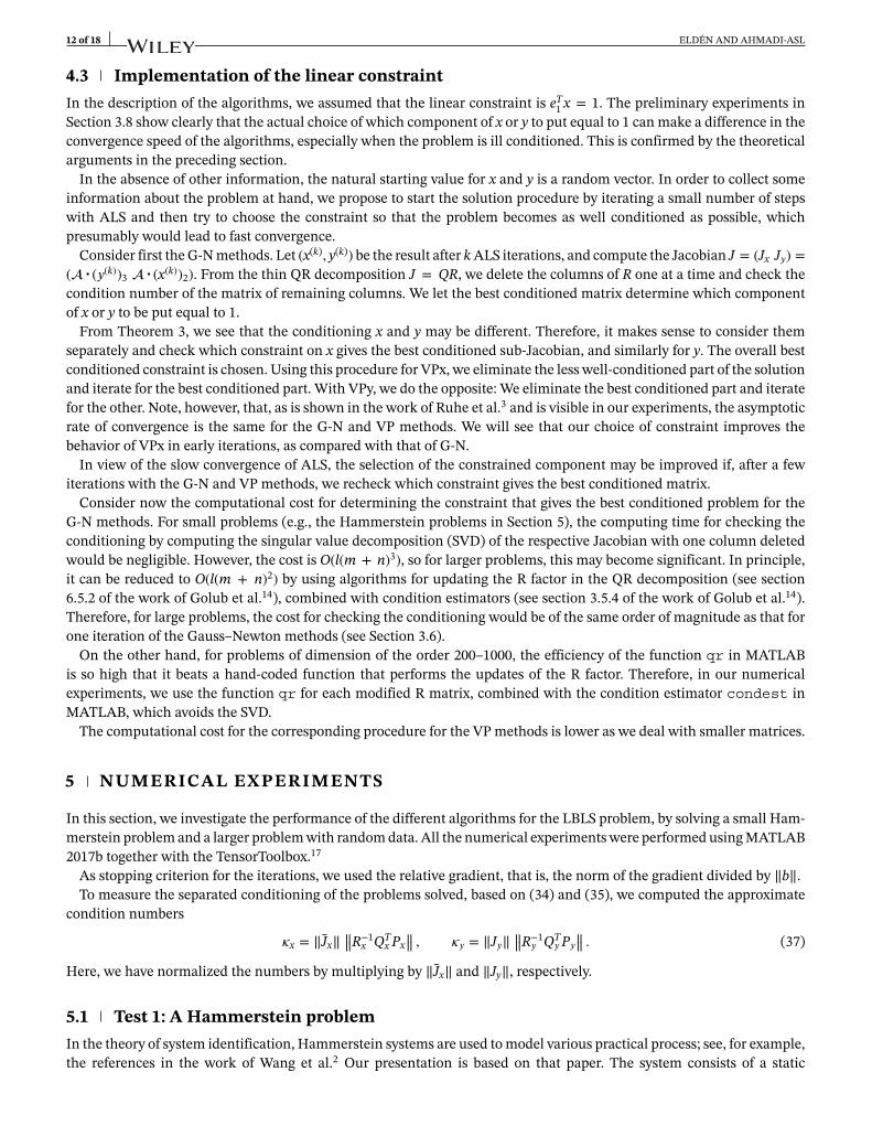
and generated the right-hand side b = · (x, 𝑦)2,3. As initial approximations, we took normally distributed vectors withmean zero and variance 1, and we started with one ALS iteration. The G-N and VP methods chose to impose the linearconstraint on the second component of y. The iterations were stopped when the relative residual was below 0.5 · 10−9. Inour first test, we had no noise (𝜏 = 0). The convergence histories are shown in Figure 2.

Clearly, the problem is very well conditioned: The approximate condition numbers (37) were of the order 407 and 1.2,respectively. With no noise, we can check the accuracy of the solution, and all relative errors were of the order 10−15 orsmaller.

We also ran the same problem with 𝜏 = 0.1. The convergence histories were very similar, except that DG-N was moreconservative and converged more slowly, in 20 iterations.

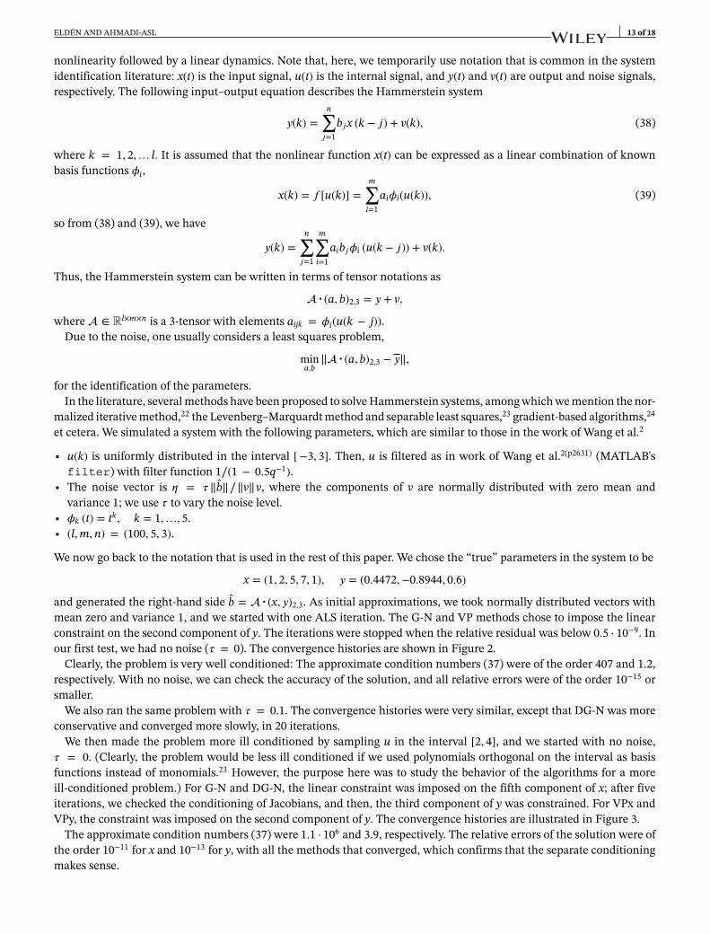
We then made the problem more ill conditioned by sampling u in the interval [2, 4], and we started with no noise,𝜏 = 0. (Clearly, the problem would be less ill conditioned if we used polynomials orthogonal on the interval as basisfunctions instead of monomials.23 However, the purpose here was to study the behavior of the algorithms for a moreill-conditioned problem.) For G-N and DG-N, the linear constraint was imposed on the fifth component of x; after fiveiterations, we checked the conditioning of Jacobians, and then, the third component of y was constrained. For VPx andVPy, the constraint was imposed on the second component of y. The convergence histories are illustrated in Figure 3.

The approximate condition numbers (37) were 1.1 · 106 and 3.9, respectively. The relative errors of the solution were ofthe order 10−11 for x and 10−13 for y, with all the methods that converged, which confirms that the separate conditioningmakes sense.

14 of 18 ELDÉN AND AHMADI-ASL

0 1 2 3 4 5 6

# iterations

10

10

10

10

10

Rel

. nor

m o

f gra

dien

t

FIGURE 2 Test 1: Well-conditioned Hammerstein problem with no noise. Convergence histories

0 1 2 3 4 5 6 7 8 9

# iterations

10

10

10

10

10

10

Rel

. nor

m o

f gra

dien

t

0 5 10 15 20 25 30

# iterations

10

10

10

10

10

10

Rel

. nor

m o

f gra

dien

t

FIGURE 3 Test 1: ill-conditioned Hammerstein problem with no noise. 𝜏 = 0 (top) and noise level 𝜏 = 0.1 (bottom). Convergence histories

ELDÉN AND AHMADI-ASL 15 of 18

We then added noise with 𝜏 = 0.1. For G-N and DG-N, the linear constraint was first imposed on the first componentof y and, then, after five iterations, on the fifth component of x. For VPx and VPy, the second component of y was con-strained. This problem is very ill conditioned: The condition number of the Hessian was of the order 1011, but it was stillpositive definite at the solution. The condition (21) was not satisfied, and the separated condition numbers (37) are nolonger relevant. The convergence was slower for the Gauss–Newton method (see the bottom plot of Figure 3). Our imple-mentation of the damped Gauss–Newton method seems to be too conservative. On the other hand, VPx takes advantageof the fact that the separated problem for y is well conditioned and converges fast.

Comparing the convergence rates in the two plots of Figure 3, we see that, for 𝜏 = 0, the Gauss–Newton and VPmethods exhibit superlinear convergence. In the case, when 𝜏 = 0.1, the convergence rate is clearly linear. The computedestimate �� of the convergence factor was of the order 0.02, which is consistent with the slope of the curves.

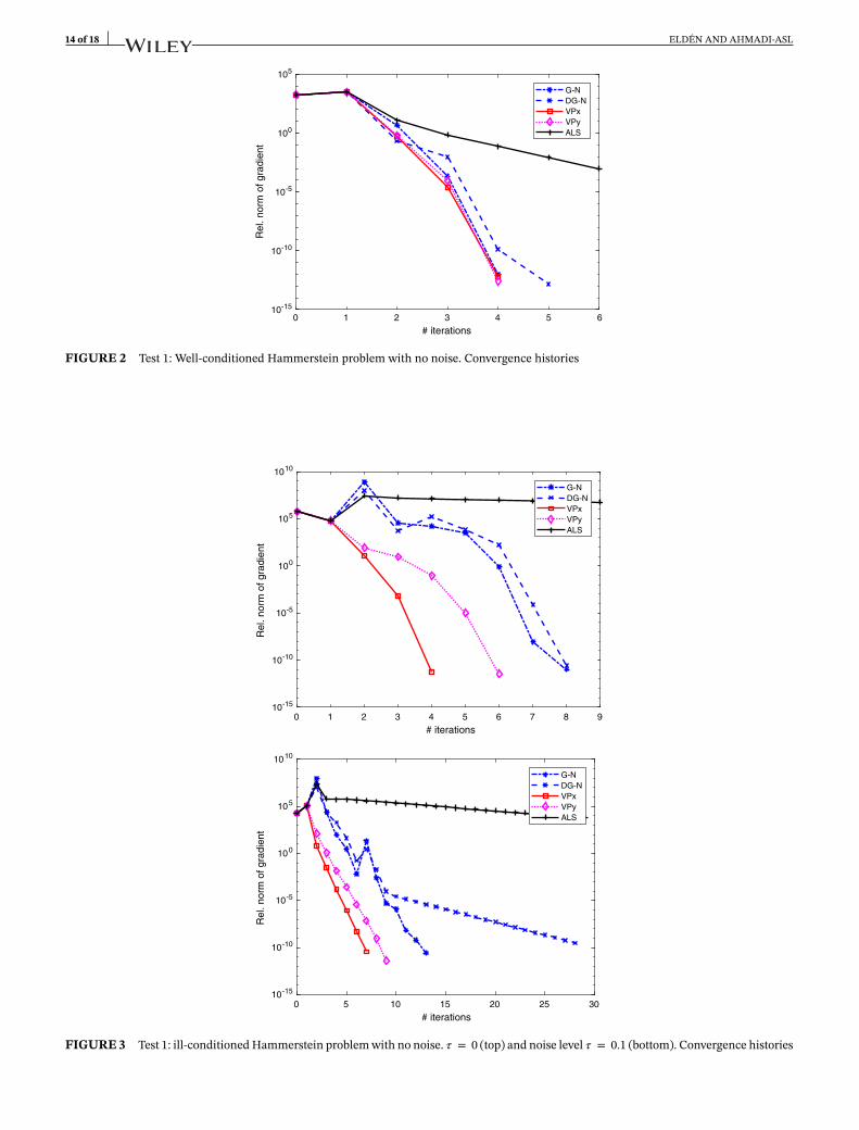
5.2 Test 2: Random dataWe let ∈ R500×200×200 be a tensor, whose elements are normally distributed N(0,1); the elements of the vectors x and yare sampled from a uniform distribution in [0, 1]. A bilinear least squares problem was constructed with right-hand side

b = b + 𝜂, b = · (x, 𝑦)2,3, 𝜂 = 𝜏 ||b|| d||d|| ,where the elements of d were normally distributed N(0,1). Before starting the iterations with the tested algorithms, weperformed three iterations of the alternating least squares method (starting from the random vectors) to get an initialapproximation. The stopping criterion was 0.5 · 10−10.

0 2 4 6 8 10 12 14

# iterations

10

10

10

10

10

Rel

. nor

m o

f gra

dien

t

0 10 20 30 40 50 60

# iterations

10

10

10

10

10

Rel

. nor

m o

f gra

dien

t

FIGURE 4 Test 2: random tensor of dimensions (500, 200, 200). Convergence histories with 𝜏 = 0.001 (top plot) and 𝜏 = 0.1 (bottom)

16 of 18 ELDÉN AND AHMADI-ASL

We first let 𝜏 = 0.001. As the solution vectors are random, it does not make sense to state which component was chosento be constrained. It is sufficient to say that, for G-N and DG-N, the constraint was first imposed on a component of y; afterfive iterations, a component of x was constrained. For VPx and VPy, a component of y was constrained. The convergenceis illustrated in Figure 4. The separated condition numbers (37) were of the order 64.

For the examples run so far, the G-N and VP methods all converged reasonably fast and it did not make sense to useNewton's method. However, for the random tensor problem with noise 𝜏 = 0.1, the convergence was considerably slower(see Figure 4). The condition number of the Hessian was of the order 5 · 103. The condition (21) was not satisfied. Theestimated convergence factor was �� = 0.69, which is consistent with the slope of the curves in Figure 4. For this problem,all methods switched constraints.

It did happen for some random tensors with 𝜏 = 0.1 that the methods converged to different solutions, correspondingto local minima. To increase robustness, we here performed six ALS iterations initially.

Here, we also tested to use Newton's method in combination with VPx. From the figure, we see that the convergencerate of VPx is linear. If we assume that the norm of the gradient is approximately Rk, where k is the iteration number and Ris the convergence rate, then we can estimate R by computing the quotient of two consecutive norms of the gradient. Fromour experience, this estimate varies in the early iterations and stabilizes as the iterations proceed. When the differencebetween these estimates for the VPx method was less than 2%, we switched to Newton iterations.

It is difficult to compare the efficiency of algorithms by timing experiments in MATLAB, due to the fact that the pro-grammer does not have control of all the aspects (especially data movement, and optimized functions vs. MATLAB code;cf. Section 3.6) that determine the speed of execution. Therefore, in order to just give a rough estimate of execution times,we here mention that the execution times for the last example were 24, 24, 21, 26, and 8.5 s, for G-N, DG-N, VPx, VPy,and VPxN, respectively (cf. Table 1). The computations were performed on a laptop computer (Intel Core i3-4030U CPU,1.90 GHz × 4) running Ubuntu Linux.

6 CONCLUSIONS AND FUTURE WORK

In this paper, we have studied different iterative methods to solve the LBLS problem. The methods were Gauss–Newtonmethods, G-N and DG-N; VP methods, VPx and VPy; Newton's method; and an alternating least squares method, ALS.Perturbation theory was presented that gave information used in the design of the algorithms. We showed that the workfor one iteration was of the same order of magnitude for all the methods, and therefore, we could make a fair compar-ison by counting the number of iterations for convergence. The methods were tested using a well-conditioned and anill-conditioned small Hammerstein identification problem and a larger artificial test problem.

Our experiments showed that, overall, the convergence of the ALS method was inferior to all the other methods.VPx converged faster and more consistently than VPy, G-N, and DG-N for the Hammerstein problems and for thewell-conditioned artificial problem. For the less well-conditioned artificial problem, with a larger data perturbation, allmethods converged more slowly. Here, we used a combination of VPx and Newton's method, which gave a dramaticallyimproved convergence rate.

The results of this paper indicate that the VP method VPx is the method of choice, possibly combined with Newton'smethod for problems with slower convergence rate. More work is needed to investigate the use of methods with close toquadratic convergence, for example, a robust variant of Newton's method. This could be especially worthwhile becauseNewton's method requires essentially the same work per iteration as the other methods. We plan to investigate this in thefuture, with emphasis on problems from actual applications.

The methods in this paper are intended for small- and medium-size problems. Large and sparse problems occur ininformation sciences; see, for example, the works of Lampos et al.10,11 We are presently studying algorithms for suchproblems. By a certain projection, the problem will be reduced to a medium-size LBLS problem, for which the methodsof this paper can be used.

More general problems, where the unknowns are matrices, for example,

minX ,Y

|| · (X ,Y )2,3 − ||,are studied in the works of Hoff9 and Lock.12 The methods of this paper can be adapted to such problems. This is a topicof our future research.

ELDÉN AND AHMADI-ASL 17 of 18

ACKNOWLEDGEMENT

We are grateful to an anonymous referee for the constructive criticism and helpful comments. The second author wassupported by the Mega Grant project (14.756.31.0001).

ORCID

Lars Eldén https://orcid.org/0000-0003-2281-856X

REFERENCES1. Bai E, Liu D. Least squares solutions of bilinear equations. Syst Control Lett. 2006;55:466–472.2. Wang J, Zhang Q, Ljung L. Revisiting Hammerstein system identification through the two-stage algorithm for bilinear parameter

estimation. Automatica. 2009;45:2627–2633.3. Ruhe A, Wedin P-Å. Algorithms for separable nonlinear least squares problems. SIAM Rev. 1980;22:318–337.4. Björck Å. Numerical methods for least squares problems. Philadelphia, PA: SIAM; 1996.5. Golub G, Pereyra V. The differentiation of pseudo-inverses and nonlinear least squares problems whose variables separate. SIAM J Numer

Anal. 1973;10:413–432.6. Ding F, Liu XP, Liu G. Identification methods for Hammerstein nonlinear systems. Digit Signal Process. 2011:21;215–238.7. Johnson CR, Smigoc H, Yang D. Solution theory for systems of bilinear equations. Lin Multilin Alg. 2014;62:1553–1566.8. Linder M, Sundberg R. Second order calibration: bilinear least squares regression and a simple alternative. Chemom Intell Lab Syst.

1998:159–178.9. Hoff PD. Multilinear tensor regression for longitudinal relational data. Ann Appl Stat. 2015:1169–1193.

10. Lampos V, Preotiuc-Pietro D, Cohn T. A user-centric model of voting intention from social media. In: Proceedings of the 51st AnnualMeeting of the Association for Computational Linguistics; 2013 Aug 4–9; Sofia, Bulgaria. Association for Computational Linguistics,Stroudsberg, PA; 2013. p. 993–1003.

11. Lampos V, Preotiuc-Pietro D, Samangooei S, Gelling D, Cohn T. Extracting socioeconomic patterns from the news: modelling text andoutlet importance jointly. In: Proceedings of the ACL 2014 Workshop on Language Technologies and Computational Social Science 2014;2014 Jun 26; Baltimore, MD. Association for Computational Linguistics, Stroudsberg, PA; 2014. p. 13–17.

12. Lock EF. Tensor-on-tensor regression. J Comput Graph Stat. 2017;27:638–647.13. Kolda TG, Bader BW. Tensor decompositions and applications. SIAM Rev. 2009;51:455–500.14. Golub G, Loan CFV. Matrix computations. 4th ed. Baltimore, MD: Johns Hopkins Press; 2013.15. Kaufman L. A variable projection method for solving separable nonlinear least squares problems. BIT Numer Math. 1975;15:49–57.16. Powell MJD. On search directions for minimization algorithms. Math Program. 1973;4:193–201.17. Bader B, Kolda T. Algorithm 862: MATLAB tensor classes for fast algorithm prototyping. ACM Trans Math Softw. 2006;32:635–653.18. Wedin P-Å. On the Gauss-Newton method for the non-linear least squares problem. Stockolm, Sweden: Institutet för Tillämpad

Matematik; 1974.19. Hansen PC. Oblique projections and standard-form transformations for discrete inverse problems. Numer Linear Algebra Appl.

2013;20:250–258.20. Szyld DB. The many proofs of an identity on the norm of oblique projections. Numer Algor. 2006;42:309–323.21. Ramsin H, Wedin P-Å. A comparison of some algorithms for the nonlinear least squares problem. BIT Numer Math. 1977;17:72–90.22. Li G, Wen C. Convergence of normalized iterative identification of Hammerstein systems. Syst Control Lett. 2011;60:929–935.23. Westwick DT, Kearney RE. Separable least squares identification of nonlinear Hammerstein models: application to stretch reflex dynamics.

Ann Biomed Eng. 2001;29:707–718.24. Ding F, Liu X, Chu J. Gradient-based and least-squares-based iterative algorithms for Hammerstein systems using the hierarchical

identification principle. IET Control Theory Appl. 2013;7:176–184.

How to cite this article: Eldén L, Ahmadi-Asl S. Solving bilinear tensor least squares problems and applicationto Hammerstein identification. Numer Linear Algebra Appl. 2018;e2226. https://doi.org/10.1002/nla.2226

APPENDIX A : DERIVATION OF THE PERTURBATION EQUATION 14

Recall that the perturbed quantity x + 𝛿x is

x + 𝛿x =(

1x

)+(

0𝛿x

). (A1)

18 of 18 ELDÉN AND AHMADI-ASL

Assume that the perturbations 𝛿 and 𝛿b satisfy (12). Consider first the perturbation of the residual,

r + 𝛿r = ( + 𝛿) · (x + 𝛿x, 𝑦 + 𝛿𝑦)2,3 − b − 𝛿b= r + · (𝛿x, 𝑦)2,3 + · (x, 𝛿𝑦)2,3 + 𝛿 · (x, 𝑦)2,3 − 𝛿b + O(𝜖2).

Ignoring O(𝜖2) and using (A1), we can write

−𝛿r + Jx𝛿x + J𝑦𝛿𝑦 = 𝛿b − 𝛿 · (x, 𝑦)2,3,

which is the first equation in (14).The perturbation of the first-order condition rTJ = 0 can be conveniently written using the notation of Section 2,

(J + 𝛿J) · (r + 𝛿r)1 = J · (r)1 + 𝛿J · (r)1 + J · (𝛿r)1 + O(𝜖2) = 0,

which, using J · (r)1 = 0 and ignoring O(𝜖2), gives

𝛿J · (r)1 + J · (𝛿r)1 = 0. (A2)

Using J = ( · (·, 𝑦)2,3 · (x, ·)2,3 ) and inserting the perturbed quantities, we get

𝛿J =( · (·, 𝛿𝑦)2,3 · (𝛿x, ·)2,3

)+(𝛿 · (·, 𝑦)2,3 𝛿 · (x, ·)2,3

)+ O(𝜖2),

and

𝛿J · (r)1 =( · (r, ·, 𝛿𝑦) · (r, 𝛿x, ·)

)+(𝛿 · (r, ·, 𝑦) 𝛿 · (r, x, ·)

)+ O(𝜖2). (A3)

Inserting J · (𝛿r)1 = ( · (𝛿r, ·, 𝑦) · (𝛿r, x, ·) ) and (A3) in (A2) and ignoring O(𝜖2), we get two equations,

· (𝛿r, 𝑦)1,3 + · (r, 𝛿𝑦)1,3 = −𝛿 · (r, 𝑦)1,3

· (𝛿r, x)1,2 + · (r, 𝛿x)1,2 = −𝛿 · (r, x)1,2.

From (A1), we have · (r, 𝛿x)1,2 = · (r, 𝛿x)1,2. Thus, translating the tensor expressions to matrix form, we have derivedthe last two equations in (14).

APPENDIX B : PROOF OF PROPOSITION 1

Proof. We put

X =(

R−1x QT

x Px

R−1𝑦 QT

𝑦P𝑦

),

and verify that the four identities uniquely defining the Moore–Penrose pseuodoinverse (see, e.g., section 5.5.2 of thework of Golub et al.14),

(i) JXJ = J, (ii) XJX = X ,(iii) JX = (JX)T , (iv) XJ = (XJ)T ,

are satisfied. Clearly, PxQx = Qx and PxQy = 0, as well as PyQy = Qy and PyQx = 0. Therefore,

XJ =

(R−1

x QTx Px

R−1𝑦 QT

𝑦P𝑦

)(QxRx Q𝑦R𝑦) =

(I 00 I

).

Thus, the identities (i), (ii), and (iv) hold. Then, we have

JX = QxQTx Px + Q𝑦QT

𝑦P𝑦.

Performing the multiplications using (32), we obtain some terms that are symmetric by inspection and the followingtwo terms:

−(Tx + T𝑦) ∶= QxF(I − FTF)−1QT𝑦 + Q𝑦FT(I − FFT)−1QT

x ,

where F = QTx Q𝑦. It is straightforward, using the SVD of F, to show that (F(I − FTF )−1)T = FT(I − FFT)−1, and

therefore, TTx = T𝑦, which implies that Tx + Ty is symmetric. This shows that (iii) holds, and the proposition is proved.