Embed Size (px)
Citation preview
arX
iv:h
ep-t
h/06
1027
3v2
6 F
eb 2
007
Solvable Critical Dense Polymers
Paul A. Pearce and Jørgen Rasmussen
Department of Mathematics and Statistics, University of Melbourne
Parkville, Victoria 3010, Australia
[email protected], [email protected]
Abstract
A lattice model of critical dense polymers is solved exactly for finite strips. The modelis the first member of the principal series of the recently introduced logarithmic minimalmodels. The key to the solution is a functional equation in the form of an inversion iden-tity satisfied by the commuting double-row transfer matrices. This is established directlyin the planar Temperley-Lieb algebra and holds independently of the space of link stateson which the transfer matrices act. Different sectors are obtained by acting on link stateswith s−1 defects where s = 1, 2, 3, . . . is an extended Kac label. The bulk and boundaryfree energies and finite-size corrections are obtained from the Euler-Maclaurin formula.The eigenvalues of the transfer matrix are classified by the physical combinatorics of thepatterns of zeros in the complex spectral-parameter plane. This yields a selection rule forthe physically relevant solutions to the inversion identity and explicit finitized charactersfor the associated quasi-rational representations. In particular, in the scaling limit, we
confirm the central charge c = −2 and conformal weights ∆s = (2−s)2−18
for s = 1, 2, 3, . . ..We also discuss a diagrammatic implementation of fusion and show with examples howindecomposable representations arise. We examine the structure of these representationsand present a conjecture for the general fusion rules within our framework.
brought to you by COREView metadata, citation and similar papers at core.ac.uk
provided by CERN Document Server
1 Introduction
Familiar materials such as plastics, nylon, polyester and plexiglass are made from poly-mers. Polymers consist of very long chain molecules with a large number of repeatingstructural units called monomers. Polymers exist in low- or high-temperature phaseswhich are characterised as either dense or dilute. Polymers are dense if they fill a finite(non-zero) fraction of the available volume in the thermodynamic limit. In this paper, weare concerned with statistical models of dense polymers in two dimensions, both on thelattice and in the continuum. From the viewpoint of lattice statistical mechanics, poly-mers are of interest as prototypical examples of systems involving (extended) non-localdegrees of freedom. It might be expected that the non-local nature of these degrees offreedom has a profound effect on the associated conformal field theory (CFT) obtainedin the continuum scaling limit. Indeed, we confirm that the associated CFT is in factlogarithmic at least in the sense that certain representations of the dilatation Virasorogenerator L0 are non-diagonalizable and exhibit Jordan cells.
A simple model [1] of linear polymers, including excluded volume effects, is basedon self-avoiding walks and can be obtained from the O(n) model in the limit n → 0.Similarly, a model [2] of branching polymers (spanning trees) is obtained from the Q-statePotts model, or more precisely the dichromatic polynomial, in the limit Q→ 0. Althoughthese approaches [3, 4, 5, 6] have yielded much insight into polymers, including thecentral charge, conformal weights and conformal characters, they rely on the propertiesof analytic continuation in n or Q.
In this paper, we propose a Yang-Baxter integrable model of critical dense polymerson the square lattice whose properties are directly accessible without the need for an-alytic continuation. In fact, this model is the first member LM(1, 2) of the principalseries of the recently introduced integrable family of logarithmic minimal models [7]. Westudy the model on a finite-width strip subject to certain boundary conditions. Remark-ably, as for the square lattice Ising model, the transfer matrices of this model satisfy asingle functional equation in the form of an inversion identity which is independent ofthe boundary conditions. This enables us to obtain the exact properties of the modelon a finite lattice. The conformal properties are then readily accessible from finite-sizecorrections. In particular, in the continuum scaling limit, we confirm the central charge
c = −2 and conformal weights ∆s = (2−s)2−18
where the extended Kac label s = 1, 2, 3, . . .labels the boundary condition. Although all of these representations appear to be diago-nalizable, we show how indecomposable representations are obtained by fusing boundaryconditions.
In contrast to simple rational CFTs, in the case of logarithmic CFTs, there can bemany different models with the same central charge and conformal weights. Specifi-cally, the logarithmic theories at c = −2 include Hamiltonian walks on a Manhattanlattice [8, 9], the rational triplet theory [10, 11, 12], symplectic fermions [13], the Abeliansandpile model [14], dimers [15], the travelling salesman problem [16] as well as branchingpolymers [17]. Although much is known about these models, it seems fair to say that at
1
present the precise relation between these various models is still not clear.The layout of this paper is as follows. In Section 2, we define our model of critical
dense polymers and the planar Temperley-Lieb (TL) algebra [18] on which it is built. InSection 3, we set up double-row transfer matrices and prove the inversion identity directlyin the planar TL algebra. We define vector spaces of link states on which the transfermatrices act and relate these to the boundary conditions. We solve the inversion identityto obtain the general solution for the eigenvalues of the transfer matrices. The physicallyrelevant solutions, in the sectors with ℓ = s − 1 defects, are obtained empirically byselection rules encoded in suitably defined double-column diagrams. In Section 4, thefinite-size corrections to the eigenvalues are obtained by applying the Euler-Maclaurinformula yielding the bulk and boundary free energies and confirming the central charge
c = −2 and conformal weights ∆s = (2−s)2−18
. In Section 5, the finitized conformalcharacters for s = 1, 2, 3, . . . are obtained explicitly from finite-width partition functionson the strip. It is also verified that these yield the quasi-rational characters of [7] in thecontinuum scaling limit. We discuss the Hamiltonian limit of the double-row transfermatrix in Section 6. In Section 7, we consider indecomposable representations. While itis well known [19] that the TL algebra admits indecomposable representations at rootsof unity, this abstract result gives no hint as to how to construct these representations onthe lattice or to relate them to physical models with physical boundary conditions. Herewe exhibit the indecomposable representations of the dilatation generator L0 arising fromthe lattice Hamiltonian and discuss how the fusion of such representations is implementedin terms of boundary conditions. The lattice approach to fusion is well established [20]in the context of boundary rational CFT and we extend the same principles here tologarithmic CFT. We conclude with some remarks and directions for future research inSection 8.
2 Lattice Model
2.1 Critical dense polymers
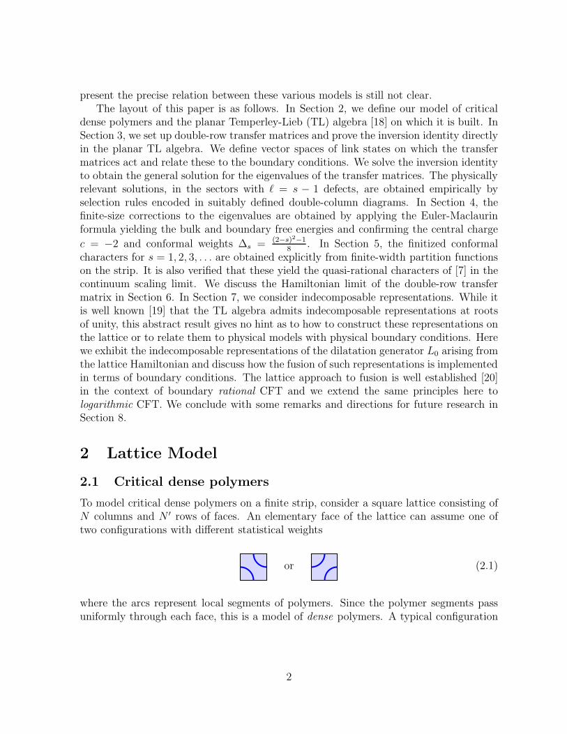
To model critical dense polymers on a finite strip, consider a square lattice consisting ofN columns and N ′ rows of faces. An elementary face of the lattice can assume one oftwo configurations with different statistical weights
or (2.1)
where the arcs represent local segments of polymers. Since the polymer segments passuniformly through each face, this is a model of dense polymers. A typical configuration
2
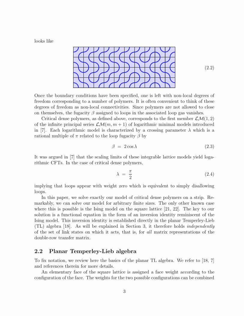
looks like
(2.2)
Once the boundary conditions have been specified, one is left with non-local degrees offreedom corresponding to a number of polymers. It is often convenient to think of thesedegrees of freedom as non-local connectivities. Since polymers are not allowed to closeon themselves, the fugacity β assigned to loops in the associated loop gas vanishes.
Critical dense polymers, as defined above, corresponds to the first member LM(1, 2)of the infinite principal series LM(m, m + 1) of logarithmic minimal models introducedin [7]. Each logarithmic model is characterized by a crossing parameter λ which is arational multiple of π related to the loop fugacity β by
β = 2 cosλ (2.3)
It was argued in [7] that the scaling limits of these integrable lattice models yield loga-rithmic CFTs. In the case of critical dense polymers,
λ =π
2(2.4)
implying that loops appear with weight zero which is equivalent to simply disallowingloops.
In this paper, we solve exactly our model of critical dense polymers on a strip. Re-markably, we can solve our model for arbitrary finite sizes. The only other known casewhere this is possible is the Ising model on the square lattice [21, 22]. The key to oursolution is a functional equation in the form of an inversion identity reminiscent of theIsing model. This inversion identity is established directly in the planar Temperley-Lieb(TL) algebra [18]. As will be explained in Section 3, it therefore holds independently
of the set of link states on which it acts, that is, for all matrix representations of thedouble-row transfer matrix.
2.2 Planar Temperley-Lieb algebra
To fix notation, we review here the basics of the planar TL algebra. We refer to [18, 7]and references therein for more details.
An elementary face of the square lattice is assigned a face weight according to theconfiguration of the face. The weights for the two possible configurations can be combined
3
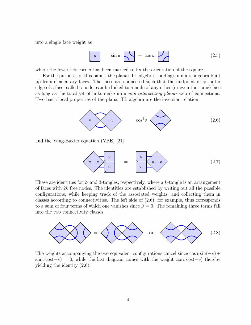
into a single face weight as
u = sin u + cos u (2.5)
where the lower left corner has been marked to fix the orientation of the square.For the purposes of this paper, the planar TL algebra is a diagrammatic algebra built
up from elementary faces. The faces are connected such that the midpoint of an outeredge of a face, called a node, can be linked to a node of any other (or even the same) faceas long as the total set of links make up a non-intersecting planar web of connections.Two basic local properties of the planar TL algebra are the inversion relation
v −v = cos2v (2.6)
and the Yang-Baxter equation (YBE) [21]
u
v
u− v =v
u
u− v (2.7)
These are identities for 2- and 3-tangles, respectively, where a k-tangle is an arrangementof faces with 2k free nodes. The identities are established by writing out all the possibleconfigurations, while keeping track of the associated weights, and collecting them inclasses according to connectivities. The left side of (2.6), for example, thus correspondsto a sum of four terms of which one vanishes since β = 0. The remaining three terms fallinto the two connectivity classes
= or (2.8)
The weights accompanying the two equivalent configurations cancel since cos v sin(−v)+sin v cos(−v) = 0, while the last diagram comes with the weight cos v cos(−v) therebyyielding the identity (2.6).
4
3 Solution on a Finite Strip
3.1 Double-row transfer matrix
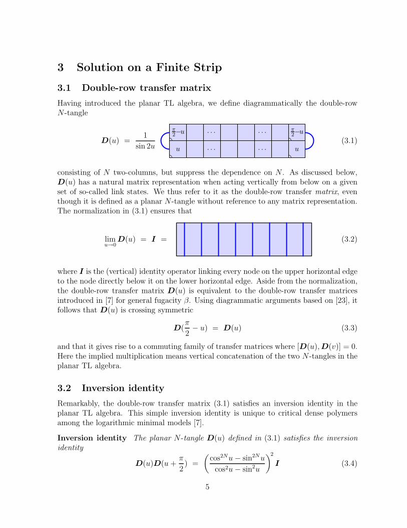
Having introduced the planar TL algebra, we define diagrammatically the double-rowN -tangle
D(u) =1
sin 2uu u
π2−u
π2−u
. . . . . .
. . . . . .
(3.1)
consisting of N two-columns, but suppress the dependence on N . As discussed below,D(u) has a natural matrix representation when acting vertically from below on a givenset of so-called link states. We thus refer to it as the double-row transfer matrix, eventhough it is defined as a planar N -tangle without reference to any matrix representation.The normalization in (3.1) ensures that
limu→0
D(u) = I = (3.2)
where I is the (vertical) identity operator linking every node on the upper horizontal edgeto the node directly below it on the lower horizontal edge. Aside from the normalization,the double-row transfer matrix D(u) is equivalent to the double-row transfer matricesintroduced in [7] for general fugacity β. Using diagrammatic arguments based on [23], itfollows that D(u) is crossing symmetric
D(π
2− u) = D(u) (3.3)
and that it gives rise to a commuting family of transfer matrices where [D(u), D(v)] = 0.Here the implied multiplication means vertical concatenation of the two N -tangles in theplanar TL algebra.
3.2 Inversion identity
Remarkably, the double-row transfer matrix (3.1) satisfies an inversion identity in theplanar TL algebra. This simple inversion identity is unique to critical dense polymersamong the logarithmic minimal models [7].
Inversion identity The planar N -tangle D(u) defined in (3.1) satisfies the inversion
identity
D(u)D(u +π
2) =
(
cos2Nu− sin2Nu
cos2u− sin2u
)2
I (3.4)
5
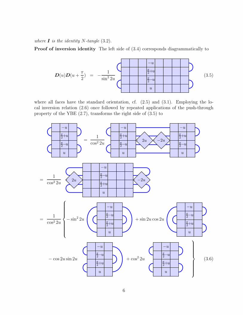
where I is the identity N-tangle (3.2).
Proof of inversion identity The left side of (3.4) corresponds diagrammatically to
D(u)D(u +π
2) = − 1
sin2 2u
u
π2−u
π2+u
−u
(3.5)
where all faces have the standard orientation, cf. (2.5) and (3.1). Employing the lo-cal inversion relation (2.6) once followed by repeated applications of the push-throughproperty of the YBE (2.7), transforms the right side of (3.5) to
u
π2−u
π2+u
−u
=1
cos2 2u
u
π2−u
π2+u
−u
u
π2−u
π2+u
−u
2u −2u
=1
cos2 2u
u
π2+u
π2−u
−u
2u −2u
=1
cos2 2u
− sin2 2u
u
π2+u
π2−u
−u
+ sin 2u cos 2u
u
π2+u
π2−u
−u
− cos 2u sin 2u
u
π2+u
π2−u
−u
+ cos2 2u
u
π2+u
π2−u
−u
(3.6)
6
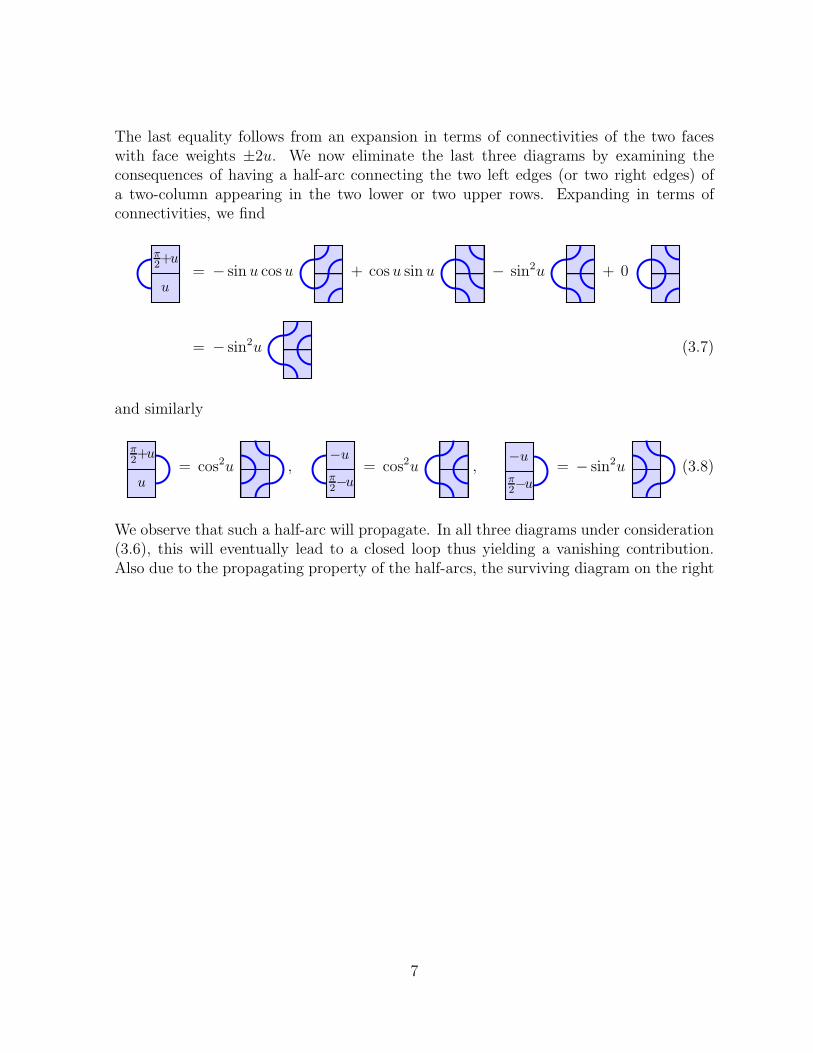
The last equality follows from an expansion in terms of connectivities of the two faceswith face weights ±2u. We now eliminate the last three diagrams by examining theconsequences of having a half-arc connecting the two left edges (or two right edges) ofa two-column appearing in the two lower or two upper rows. Expanding in terms ofconnectivities, we find
π2+u
u
= − sin u cosu + cos u sin u − sin2u + 0
= − sin2u (3.7)
and similarly
π2+u
u
= cos2u ,π2−u
−u
= cos2u ,π2−u
−u= − sin2u (3.8)
We observe that such a half-arc will propagate. In all three diagrams under consideration(3.6), this will eventually lead to a closed loop thus yielding a vanishing contribution.Also due to the propagating property of the half-arcs, the surviving diagram on the right
7
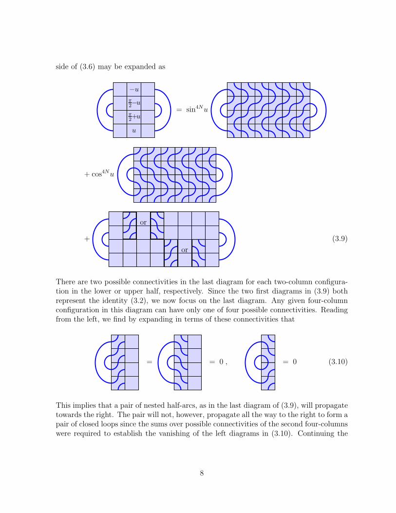
side of (3.6) may be expanded as
u
π2+u
π2−u
−u
= sin4Nu
+ cos4Nu
+
or
or
(3.9)
There are two possible connectivities in the last diagram for each two-column configura-tion in the lower or upper half, respectively. Since the two first diagrams in (3.9) bothrepresent the identity (3.2), we now focus on the last diagram. Any given four-columnconfiguration in this diagram can have only one of four possible connectivities. Readingfrom the left, we find by expanding in terms of these connectivities that
= = 0 , = 0 (3.10)
This implies that a pair of nested half-arcs, as in the last diagram of (3.9), will propagatetowards the right. The pair will not, however, propagate all the way to the right to form apair of closed loops since the sums over possible connectivities of the second four-columnswere required to establish the vanishing of the left diagrams in (3.10). Continuing the
8
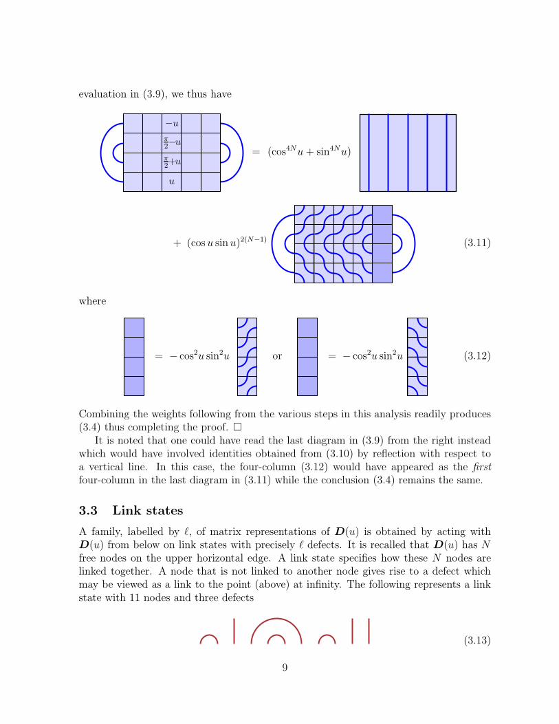
evaluation in (3.9), we thus have
u
π2+u
π2−u
−u
= (cos4Nu + sin4Nu)
+ (cos u sinu)2(N−1) (3.11)
where
= − cos2u sin2u or = − cos2u sin2u (3.12)
Combining the weights following from the various steps in this analysis readily produces(3.4) thus completing the proof. �
It is noted that one could have read the last diagram in (3.9) from the right insteadwhich would have involved identities obtained from (3.10) by reflection with respect toa vertical line. In this case, the four-column (3.12) would have appeared as the first
four-column in the last diagram in (3.11) while the conclusion (3.4) remains the same.
3.3 Link states
A family, labelled by ℓ, of matrix representations of D(u) is obtained by acting withD(u) from below on link states with precisely ℓ defects. It is recalled that D(u) has Nfree nodes on the upper horizontal edge. A link state specifies how these N nodes arelinked together. A node that is not linked to another node gives rise to a defect whichmay be viewed as a link to the point (above) at infinity. The following represents a linkstate with 11 nodes and three defects
(3.13)
9
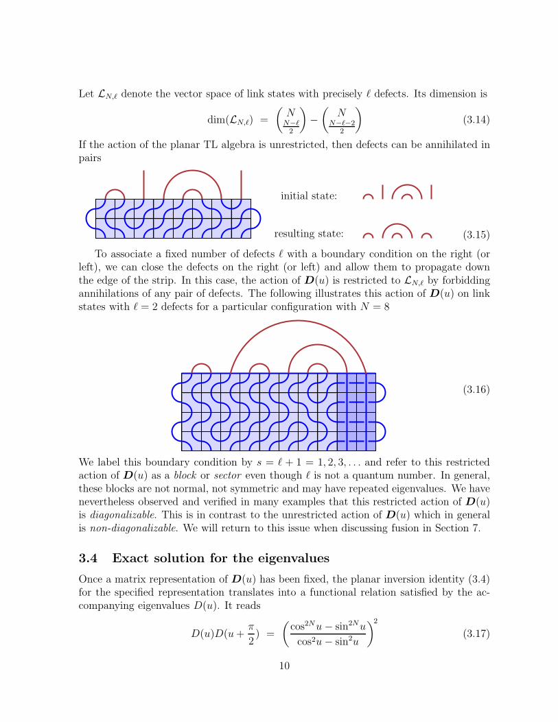
Let LN,ℓ denote the vector space of link states with precisely ℓ defects. Its dimension is
dim(LN,ℓ) =
(
NN−ℓ
2
)
−(
NN−ℓ−2
2
)
(3.14)
If the action of the planar TL algebra is unrestricted, then defects can be annihilated inpairs
initial state:
resulting state: (3.15)
To associate a fixed number of defects ℓ with a boundary condition on the right (orleft), we can close the defects on the right (or left) and allow them to propagate downthe edge of the strip. In this case, the action of D(u) is restricted to LN,ℓ by forbiddingannihilations of any pair of defects. The following illustrates this action of D(u) on linkstates with ℓ = 2 defects for a particular configuration with N = 8
(3.16)
We label this boundary condition by s = ℓ + 1 = 1, 2, 3, . . . and refer to this restrictedaction of D(u) as a block or sector even though ℓ is not a quantum number. In general,these blocks are not normal, not symmetric and may have repeated eigenvalues. We havenevertheless observed and verified in many examples that this restricted action of D(u)is diagonalizable. This is in contrast to the unrestricted action of D(u) which in generalis non-diagonalizable. We will return to this issue when discussing fusion in Section 7.
3.4 Exact solution for the eigenvalues
Once a matrix representation of D(u) has been fixed, the planar inversion identity (3.4)for the specified representation translates into a functional relation satisfied by the ac-companying eigenvalues D(u). It reads
D(u)D(u +π
2) =
(
cos2Nu− sin2Nu
cos2u− sin2u
)2
(3.17)
10
where the normalization (3.2) and the crossing symmetry (3.3) yield the conditions
D(0) = 1, D(π
2− u) = D(u) (3.18)
The analysis of (3.17) depends on the parity of N as we have the factorization
cos2Nu− sin2Nu
cos2u− sin2u=
N
2N−1
N2−1
∏
j=1
( 1
sin2 jπN
− sin2 2u)
, N even
1
2N−1
N−12
∏
j=1
( 1
sin2 (2j−1)π2N
− sin2 2u)
, N odd
(3.19)
It is now straightforward to solve the functional relation (3.17), subject to (3.18), bysharing out the zeros. We find
D(u) =
N
2N−1
N2−1
∏
j=1
( 1
sin jπN
+ ǫj sin 2u)( 1
sin jπN
+ µj sin 2u)
, N even
1
2N−1
N−12
∏
j=1
( 1
sin (2j−1)π2N
+ ǫj sin 2u)( 1
sin (2j−1)π2N
+ µj sin 2u)
, N odd
(3.20)
where ǫ2j = µ2
j = 1 for all j. The appearance of two sets of parameters {ǫj} and {µj}stems from the overall squaring in (3.17).
For either parity of N in (3.20), the maximum eigenvalue is obtained for ǫj = µj = 1for all j and corresponds to the ground state in the associated sector. Excited statesare generated by switching a (finite) number of the parameters ǫj , µj from 1 to −1.The number of possible excitations following from (3.20) is 2N−2 and 2N−1, respectively,clearly exceeding the number of link states with a definite number of defects, cf. (3.14).We thus need a set of selection rules to determine which eigenvalues actually appear inthe spectrum and therefore are physical. This information is neatly encoded by specifyingthe patterns of complex zeros of D(u) which are allowed.
Generally, the zeros of an eigenvalue D(u) come in conjugate pairs in the complexu-plane and appear with a periodicity π in the real part of u. They follow from (3.20)and are collectively described by
u ∈{
(2 + νj)π
4± i
2ln tan
tj2
}
+ πZ (3.21)
where νj is ǫj or µj, and where we have introduced the arguments
tj =
{ jπN
, N even
(2j−1)π2N
, N odd(3.22)
11
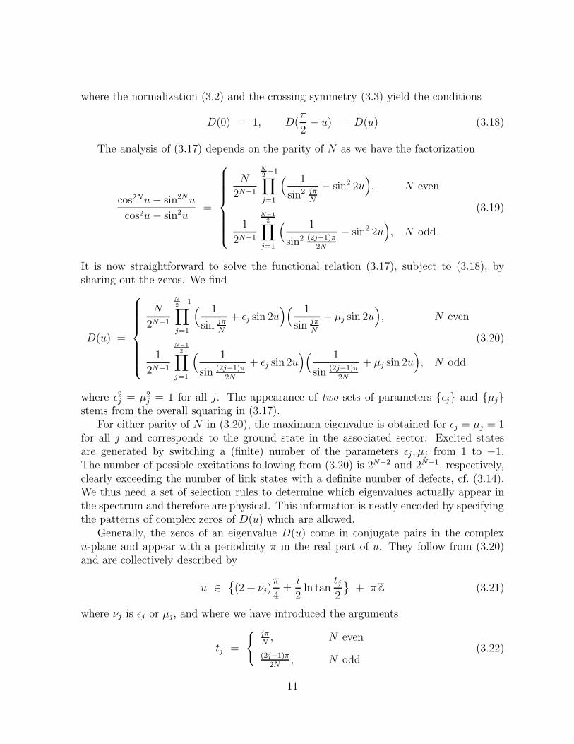
A typical pattern for N = 12 is
−π4
π4
π2
3π4
y5
y4
y3
y2
y1
−y5
−y4
−y3
−y2
−y1
(3.23)
where
yj = − i
2ln tan
tj2
(3.24)
The infinite analyticity strip bounded by u = −π4
and u = 3π4
is called the physicalstrip. All zeros in the strip lie either on the boundary or on the vertical centre line(1-strings). In contrast to the usual situation in the context of Bethe ansatz, these zeroscan occur either as single or double zeros. A single zero is indicated by a grey dot whilea double zero is indicated by a black dot. Counting a double zero twice, the number ofzeros with fixed imaginary value ±yj and real part either π
4or 3π
4is two. This follows
straightforwardly from (3.21) since νj can be either ǫj or µj , as depicted in (3.23). Thefact that the zeros appear in complex conjugate pairs is now seen to be a consequence ofthe crossing symmetry (3.18) and the periodicity in the u-plane.
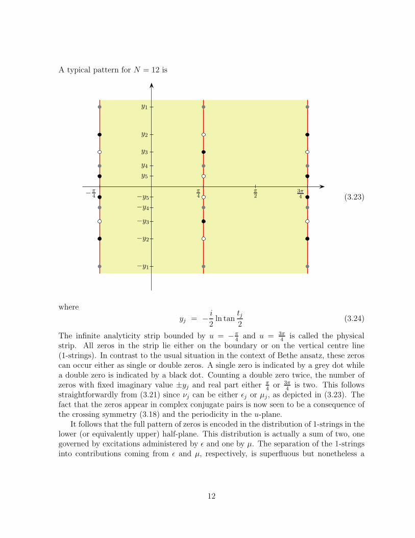
It follows that the full pattern of zeros is encoded in the distribution of 1-strings in thelower (or equivalently upper) half-plane. This distribution is actually a sum of two, onegoverned by excitations administered by ǫ and one by µ. The separation of the 1-stringsinto contributions coming from ǫ and µ, respectively, is superfluous but nonetheless a
12
helpful refinement later for the description of the selection rules. It is illustrated here
←→ (3.25)
where the left side corresponds to (3.23) while the two columns to the right encode sepa-rately the ǫ and µ excitations. Not all such double-column configurations will appear. Acharacterization of a set of admissible two-column configurations provides a descriptionof the selection rules. This combinatorial designation of the physical states is termed‘physical combinatorics’. The details of the combinatorial content is the topic of ourforthcoming paper [24]. A synopsis follows below and is used in our description of theselection rules to be discussed subsequently. As we will see, the double-column configu-rations also provide a natural basis for defining the associated finitized characters.
3.5 Double-column configurations
A single-column configuration of height M consists of M sites arranged as a column. Thesites are labelled from the bottom by the integers 1, . . . , M and are weighted accordinglyby 1, . . . , M . A site can be occupied or unoccupied. The signature S of a single-columnconfiguration is constructed as the set of weights of the occupied sites in the configurationlisted in descending order. The weight w of a configuration is given by the sum of thesignature entries
w(S) =∑
j
Sj (3.26)
A double-column configuration of height M consists of a pair of single-column config-urations of height M . The notions of signature and weight are readily extended from thesingle-column case as illustrated by the right side of (3.25). It has weight w = 11 whilethe signature is
S = (L, R), L = (3), R = (4, 3, 1) (3.27)
Here L and R refer to the signatures of the left and right single-column configurations,respectively. With m and n indicating the number of occupied sites in the left and rightcolumns, respectively, the weight w of a double-column configuration is given by
w(L, R) =
m∑
j=1
Lj +
n∑
j=1
Rj (3.28)
The set of single-column configurations of height M admits the partial ordering
S � S ′ if Sj ≤ S ′j, j = 1, . . . , m (3.29)
13
where S and S ′ are two such single-column configurations with m and m′ occupied sites,respectively. A double-column configuration with signature S = (L, R) is called admissi-
ble if L � R. This presupposes, in particular, that
0 ≤ m ≤ n ≤ M (3.30)
The configuration (3.25) is seen to be admissible. This convention for admissibility cor-responds to µ being dominant over ǫ. We let AM
m,n denote the set of admissible double-column configurations with m occupied sites in the left column and n occupied sites in theright column. It is noted that the set AM
m,n is empty if and only if one of the inequalities(3.30) is violated.
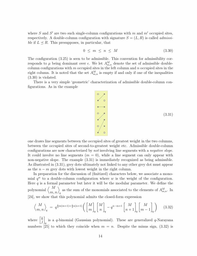
There is a very simple ‘geometric’ characterization of admissible double-column con-figurations. As in the example
(3.31)
one draws line segments between the occupied sites of greatest weight in the two columns,between the occupied sites of second-to-greatest weight etc. Admissible double-columnconfigurations are now characterized by not involving line segments with a negative slope.It could involve no line segments (m = 0), while a line segment can only appear withnon-negative slope. The example (3.31) is immediately recognized as being admissible.As illustrated in (3.31), grey dots ultimately not linked to any other grey dot must appearas the n−m grey dots with lowest weight in the right column.
In preparation for the discussion of (finitized) characters below, we associate a mono-mial qw to a double-column configuration where w is the weight of the configuration.Here q is a formal parameter but later it will be the modular parameter. We define the
polynomial⟨ M
m, n
⟩
qas the sum of the monomials associated to the elements of AM
m,n. In
[24], we show that this polynomial admits the closed-form expression
⟨
Mm, n
⟩
q= q
12m(m+1)+ 1
2n(n+1)
( [
Mm
]
q
[
Mn
]
q
− qn−m+1
[
Mn + 1
]
q
[
Mm− 1
]
q
)
(3.32)
where[
kj
]
qis a q-binomial (Gaussian polynomial). These are generalized q-Narayana
numbers [25] to which they coincide when m = n. Despite the minus sign, (3.32) is
14
actually fermionic in the sense that it is a polynomial with only non-negative coefficients[24].
3.6 Selection rules
We now turn to the description of the selection rules. They depend on the parity ofN . Based on a body of empirical data obtained by examining the double-row transfermatrices analytically as well as numerically, we make the following conjecture.
Selection rules For a system with N columns and ℓ defects where N− ℓ ≡ 0 mod 2, the
selection rules are equivalent to singling out the following sets of admissible double-column
configurations
N even :
N−ℓ2
⋃
m=0
(
AN−2
2
m,m+ ℓ−22
∪ AN−2
2
m,m+ ℓ2
)
, N odd :
N−ℓ2
⋃
m=0
AN−1
2
m,m+ ℓ−12
(3.33)
By construction, all these unions are disjoint unions. It is noted that the case where
ℓ = 0 is special since AN−2
2m,m−1 = ∅. As argued below, ℓ = 0 gives rise to the identity field
in the associated CFT.
4 Finite-Size Corrections
The partition function of critical dense polymers on a lattice of N columns and M doublerows is defined by
ZN,M = Tr D(u)M =∑
n
Dn(u)M =∑
n
e−MEn(u) (4.1)
where the sum is over all eigenvalues of D(u) including possible multiplicities and En(u)is the energy associated to the eigenvalue Dn(u). A refinement of (4.1) to treat explicitlysectors with different numbers of defects is given in the next section. Conformal invarianceof the model in the continuum scaling limit would dictate [26, 27] that the leading finite-size corrections for large N are of the form
En(u) = − ln Dn(u) ≃ 2Nfbulk + fbdy +2π sin 2u
N
(
− c
24+ ∆ + k
)
(4.2)
Here fbulk is the bulk free energy per face, fbdy is the boundary or surface free energy, whilec is the central charge of the CFT whose spectrum of conformal weights is given by thepossible values of ∆ with excitations or descendants labelled by the non-negative integersk. As the analysis below will confirm, the asymptotic behaviour of the eigenvalues (3.20)are in accordance with (4.2).
15
The logarithms of the eigenvalues (3.20) involves sums of terms which are singular inthe limit N →∞. To remedy this, one can introduce the function
F (t) = ln( t
sin t+ t sin 2u
)
= ln t + ln( 1
sin t+ sin 2u
)
(4.3)
which is well defined as t → 0 and where the u dependence for simplicity has beenformally suppressed. This trick was employed in a similar analysis [22] of the Isingmodel, and it allows us to examine the asymptotic behaviour of the logarithms. Indeed,the Euler-Maclaurin formula now gives
m∑
k=0
F (a + kh) ≃ 1
h
∫ b
a
F (t)dt +1
2[F (b) + F (a)] +
h
12[F ′(b)− F ′(a)] (4.4)
where b = a + mh, and due to the split (4.3), we also need to approximate the logarithmof the gamma function
ln Γ(y) ≃ (y − 12) ln y − y + 1
2ln(2π) +
1
12y(4.5)
As a partial evaluation of the energies (4.2), we find
ln∏
j
( 1
sin tj+ ǫj sin 2u
)
≃∑
j
(
F (tj)− ln tj)
− 2 sin 2u∑
j∈E
tj (4.6)
where E is the subset of j indices for which ǫj = −1 and E remains finite as N → ∞.Likewise, M denotes the subset of j indices for which µj = −1 and it also remains finiteas N →∞. The argument tj is defined in (3.22). We finally find
En(u) ≃ 2Nfbulk + fbdy
+2π sin 2u
N
( 2
24+
∑
j∈EN,n
j +∑
j∈MN,n
j)
, N even
( 2
24− 1
8+
∑
j∈EN,n
(j − 12) +
∑
j∈MN,n
(j − 12))
, N odd
(4.7)
In these expressions, the bulk free energy per face is given by
fbulk = ln√
2− 1
π
∫ π/2
0
ln( 1
sin t+ sin 2u
)
dt (4.8)
whereas the boundary free energy is given by
fbdy = ln(1 + sin 2u) (4.9)
16
5 Conformal Field Theory
The next task and our main objective is to calculate analytically the conformal dataassociated with our model of critical dense polymers. By comparing the expressions (4.7)with the finite-size corrections (4.2), the central charge is readily seen to be
c = −2 (5.1)
while the lowest conformal weights for given parity of N are ∆ = 0 and ∆ = −18,
respectively. The full spectrum of conformal weights and their excitations are discussedin the following.
5.1 Finitized characters
It is recalled that the matrix representation of the double-row transfer matrix dependson which space D(u) is acting. Since the action of D(u) on LN is upper block-triangular,the partition function (4.1) may be written
ZN,M =∑
s
∑
n
D(s)n (u)M =
∑
s
∑
n
e−ME(s)n (u) (5.2)
where D(s)n (u) and E
(s)n (u) are the eigenvalues and associated energies obtained by re-
stricting to the ℓ = s− 1 sector. Likewise, information on the excitations or descendantsare contained in the appropriate sets E (s)
N,n andM(s)N,n, cf. (4.7). Here we have introduced
the extended Kac label s related to the number of defects ℓ by
s = ℓ + 1 (5.3)
Now, the link between the lattice model and the characters of the CFT is governedby the modular parameter q defined by
q = e−2πτ , τ =M
Nsin 2u (5.4)
The ratio M/N is the aspect ratio and ϑ = 2u is the anisotropy angle related to thegeometry of the lattice. As already discussed, the spectrum of the CFT is extracted fromthe eigenvalues, that is, the specification of E (s)
N,n and M(s)N,n for all s. This amounts to
determining appropriate selection rules. The relevant rules are stated explicitly in (3.33)where ℓ = s− 1.
For finite N , we thus find that the full spectrum can be organized in finitized charactersχ(N)
s (q) and we find that they are given by
χ(N)s (q) =
q112
N−s+12
∑
m=0
(⟨ N−22
m, m + s−32
⟩
q+
⟨ N−22
m, m + s−12
⟩
q
)
, s odd
q−124
− s−24
N−s+12
∑
m=0
⟨ N−12
m, m + s−22
⟩
qq−m, s even
(5.5)
17
where some terms may vanish, cf. (3.30). It is emphasized that these are fermionic
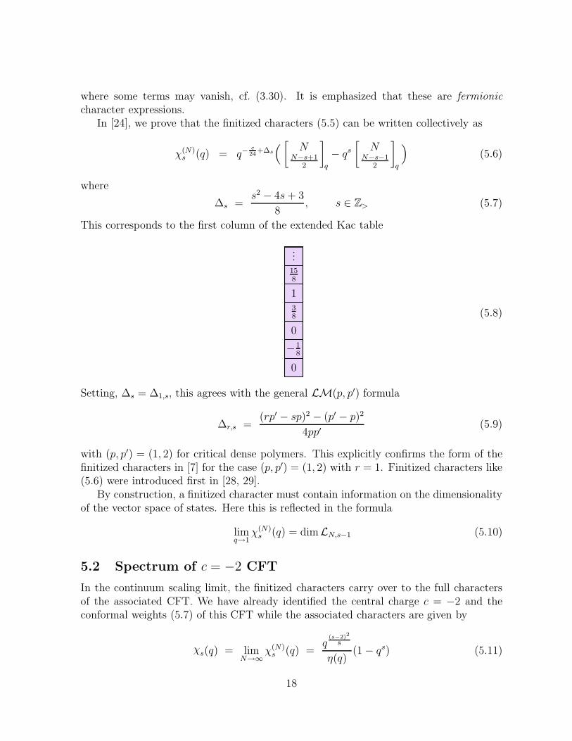
character expressions.In [24], we prove that the finitized characters (5.5) can be written collectively as
χ(N)s (q) = q−
c24
+∆s
(
[
NN−s+1
2
]
q
− qs
[
NN−s−1
2
]
q
)
(5.6)
where
∆s =s2 − 4s + 3
8, s ∈ Z> (5.7)
This corresponds to the first column of the extended Kac table
0
−18
0
38
1
158
...
(5.8)
Setting, ∆s = ∆1,s, this agrees with the general LM(p, p′) formula
∆r,s =(rp′ − sp)2 − (p′ − p)2
4pp′(5.9)
with (p, p′) = (1, 2) for critical dense polymers. This explicitly confirms the form of thefinitized characters in [7] for the case (p, p′) = (1, 2) with r = 1. Finitized characters like(5.6) were introduced first in [28, 29].
By construction, a finitized character must contain information on the dimensionalityof the vector space of states. Here this is reflected in the formula
limq→1
χ(N)s (q) = dimLN,s−1 (5.10)
5.2 Spectrum of c = −2 CFT
In the continuum scaling limit, the finitized characters carry over to the full charactersof the associated CFT. We have already identified the central charge c = −2 and theconformal weights (5.7) of this CFT while the associated characters are given by
χs(q) = limN→∞
χ(N)s (q) =
q(s−2)2
8
η(q)(1− qs) (5.11)
18
where the Dedekind eta function is defined by
η(q) = q124
∞∏
m=1
(1− qm) (5.12)
The character χs(q) is recognized as the Virasoro character of a particular quasi-rational highest-weight representation of the Virasoro algebra. To appreciate this, werecall that the Verma module Vr,s of a Virasoro highest-weight representation of highestweight (5.9) is defined for all r, s ∈ Z> and p, p′ two coprime positive integers. Theassociated quotient module
Qr,s = Vr,s/Vr,−s (5.13)
is also defined for every pair of positive integers r, s and corresponds to a quasi-rationalrepresentation. The character of such a quasi-rational representation is given by
χr,s(q) =q
1−c24
η(q)
(
q∆r,s − q∆r,−s)
=q
1−c24
η(q)q∆r,s (1− qrs)
where c = 1 − 6 (p′−p)2
pp′. Critical dense polymers correspond to (p, p′) = (1, 2) in which
case χ1,s(q) = χs(q), as already indicated.So far for critical dense polymers, from the lattice approach, we have only identified
sectors with r = 1. The associated quasi-rational characters correspond to representa-tions (1, s) which are only irreducible for s = 1 or s even. From the point of view of CFT,one conventionally works with irreducible representations as the natural building blocks.This is indeed the case in [30] where the complete set of irreducible representations nec-essarily involve sectors corresponding to r > 1, even after identification of irreduciblerepresentations with identical characters following the classification of irreducible char-acters in the appendix of [7]. A lattice analysis of the set of irreducible representationswill appear elsewhere.
A variety of character identities exist for the set of quasi-rational representations. Inparticular, every quasi-rational character (5.14) with r > 1 can be written as a linearcombination of characters with r = 1
χ1+k,s(q) =k
∑
j=0
χs+4j−2k(q) (5.14)
where it is implicit that
χ0(q) = 0, χ−s(q) = −χs(q) (5.15)
This extends to general r, s and coprime p, p′ [24] by admitting linear combinations ofthe p left-most columns in the extended Kac table
χr+kp,s(q) =k
∑
j=0
χr,s+(2j−k)p′(q) +k−1∑
j=0
χp−r,s+(2j+1−k)p′(q) (5.16)
employing a straightforward extension of (5.15). It is emphasized, though, that thesecharacter identities are blind to any Jordan cells, cf. Section 7.
19
6 Hamiltonian Limit
The Hamiltonian limit of the double-row transfer matrix D(u) is defined in the planaralgebra as the N -tangle appearing as the leading non-trivial term in an expansion withrespect to u, that is,
D(u) = I − 2uH + O(u2) (6.1)
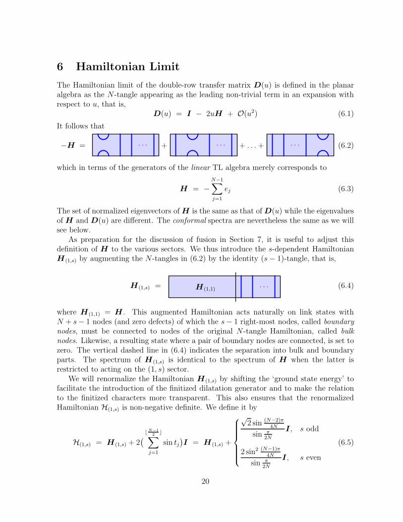
It follows that
−H = . . . + . . . + . . . + . . . (6.2)
which in terms of the generators of the linear TL algebra merely corresponds to
H = −N−1∑
j=1
ej (6.3)
The set of normalized eigenvectors of H is the same as that of D(u) while the eigenvaluesof H and D(u) are different. The conformal spectra are nevertheless the same as we willsee below.
As preparation for the discussion of fusion in Section 7, it is useful to adjust thisdefinition of H to the various sectors. We thus introduce the s-dependent HamiltonianH(1,s) by augmenting the N -tangles in (6.2) by the identity (s− 1)-tangle, that is,
H(1,s) = H(1,1). . . (6.4)
where H(1,1) = H . This augmented Hamiltonian acts naturally on link states withN + s− 1 nodes (and zero defects) of which the s− 1 right-most nodes, called boundary
nodes, must be connected to nodes of the original N -tangle Hamiltonian, called bulk
nodes. Likewise, a resulting state where a pair of boundary nodes are connected, is set tozero. The vertical dashed line in (6.4) indicates the separation into bulk and boundaryparts. The spectrum of H(1,s) is identical to the spectrum of H when the latter isrestricted to acting on the (1, s) sector.
We will renormalize the Hamiltonian H(1,s) by shifting the ‘ground state energy’ tofacilitate the introduction of the finitized dilatation generator and to make the relationto the finitized characters more transparent. This also ensures that the renormalizedHamiltonian H(1,s) is non-negative definite. We define it by
H(1,s) = H(1,s) + 2(
⌊N−12
⌋∑
j=1
sin tj)
I = H(1,s) +
√2 sin (N−2)π
4N
sin π2N
I, s odd
2 sin2 (N−1)π4N
sin π2N
I, s even
(6.5)
20
where tj is defined in (3.22), and find that its eigenvalues are given by
2∑
j∈E(s)N
sin tj + 2∑
j∈M(s)N
sin tj (6.6)
Since the eigenvalues of H(1,s) can be expressed as the linear combinations (6.6) of
terms like sin tj , we may now define the finitized dilatation generator L(1,s)0 by replacing
these summands sin tj by Ntj/2π in the Jordan canonical form of H(1,s)− 1+(−1)s
16I when
the diagonal entries of the latter are expressed as in (6.6). That is, we are defining thefinitized dilatation generator by the formal replacement
L(1,s)0 = Jordan
(
H(1,s) −1 + (−1)s
16I
)
∣
∣
∣
∣
∣
sin tj 7→Ntj
2π
(6.7)
The dependence on N has been suppressed. An eventual off-diagonal part of this Jordancanonical form is unaltered by this replacement. We observe, though, that the Hamilto-nian H(1,s) is diagonalizable. This is in accordance with our observation in Section 3.3that the double-row transfer matrix D(u) itself is diagonalizable when restricted to thesector (1, s). In the discussion of fusion in Section 7, on the other hand, we will encounterHamiltonians which are not diagonalizable.
It also follows that the eigenvalues of L(1,s)0 are
∑
j∈E(s)N
j +∑
j∈M(s)N
j, s odd
−1
8+
∑
j∈E(s)N
(j − 12) +
∑
j∈M(s)N
(j − 12), s even (6.8)
in accordance with (4.7). This confirms the assertion above that the double-row transfermatrix and the Hamiltonian have the same conformal spectra. We can also re-expressthe finitized characters as
χ(N)1,s (q) = Tr qL
(1,s)0 −c/24 (6.9)
thus mimicking the definition of the ordinary Virasoro characters.
7 Fusion
In this section, we explain the diagrammatic implementation of fusion within our frame-work [7]. Although we focus here on critical dense polymers and the sectors with r = 1(labelled by s = 1, 2, . . .), the construction extends to the other logarithmic minimalmodels and sectors with r > 1, albeit with more involved computations. For conveniencein the description of our fusion prescription, we work with the Hamiltonian limit of thedouble-row transfer matrix. The conclusions about fusion are the same but more tediousto reach when the analysis is based on the double-row transfer matrix D(u) itself.
21
7.1 Fusion prescription
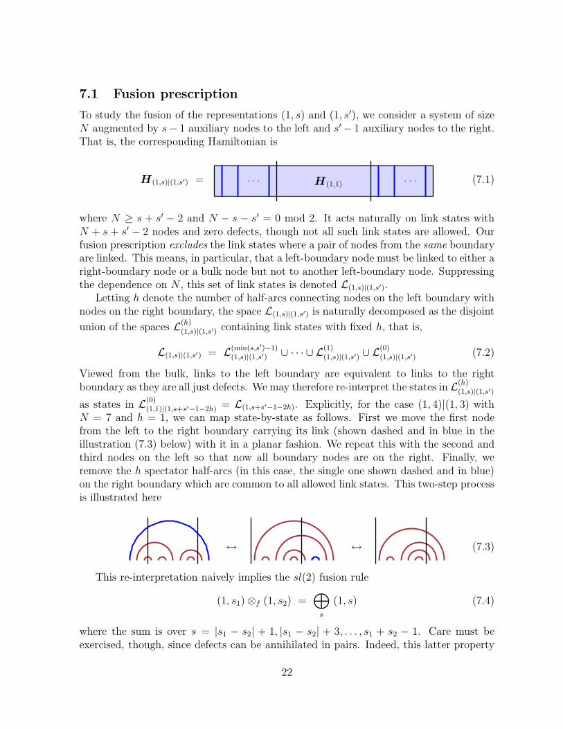
To study the fusion of the representations (1, s) and (1, s′), we consider a system of sizeN augmented by s− 1 auxiliary nodes to the left and s′− 1 auxiliary nodes to the right.That is, the corresponding Hamiltonian is
H(1,s)|(1,s′) = . . . H(1,1). . . (7.1)
where N ≥ s + s′ − 2 and N − s − s′ = 0 mod 2. It acts naturally on link states withN + s + s′ − 2 nodes and zero defects, though not all such link states are allowed. Ourfusion prescription excludes the link states where a pair of nodes from the same boundaryare linked. This means, in particular, that a left-boundary node must be linked to either aright-boundary node or a bulk node but not to another left-boundary node. Suppressingthe dependence on N , this set of link states is denoted L(1,s)|(1,s′).
Letting h denote the number of half-arcs connecting nodes on the left boundary withnodes on the right boundary, the space L(1,s)|(1,s′) is naturally decomposed as the disjoint
union of the spaces L(h)(1,s)|(1,s′) containing link states with fixed h, that is,
L(1,s)|(1,s′) = L(min(s,s′)−1)(1,s)|(1,s′) ∪ · · · ∪ L(1)
(1,s)|(1,s′) ∪ L(0)(1,s)|(1,s′) (7.2)
Viewed from the bulk, links to the left boundary are equivalent to links to the rightboundary as they are all just defects. We may therefore re-interpret the states in L(h)
(1,s)|(1,s′)
as states in L(0)(1,1)|(1,s+s′−1−2h) = L(1,s+s′−1−2h). Explicitly, for the case (1, 4)|(1, 3) with
N = 7 and h = 1, we can map state-by-state as follows. First we move the first nodefrom the left to the right boundary carrying its link (shown dashed and in blue in theillustration (7.3) below) with it in a planar fashion. We repeat this with the second andthird nodes on the left so that now all boundary nodes are on the right. Finally, weremove the h spectator half-arcs (in this case, the single one shown dashed and in blue)on the right boundary which are common to all allowed link states. This two-step processis illustrated here
↔ ↔ (7.3)
This re-interpretation naively implies the sl(2) fusion rule
(1, s1)⊗f (1, s2) =⊕
s
(1, s) (7.4)
where the sum is over s = |s1 − s2| + 1, |s1 − s2| + 3, . . . , s1 + s2 − 1. Care must beexercised, though, since defects can be annihilated in pairs. Indeed, this latter property
22
implies that the action of the Hamiltonian on (7.2) is upper block-triangular rather thanblock-diagonal. There is thus the possibility of forming indecomposable representations inwhich case the right side of (7.4) is not a direct sum. In the following, we will characterizethese representations and conjecture the fusion rules applying to the complete set ofrepresentations generated by fusion of the (1, s) building blocks.
Due to the decomposition (7.2), the renormalization of the Hamiltonian H (1,s)|(1,s′) isdefined as in (6.5) by
H(1,s)|(1,s′) = H(1,s)|(1,s′) +
√2 sin (N−2)π
4N
sin π2N
I, s + s′ even
2 sin2 (N−1)π4N
sin π2N
I, s + s′ odd
(7.5)
Due to the decomposition (7.2) and the subsequent re-interpretation, the eigenvalues ofH(1,s)|(1,s′) are
2∑
j∈E(s+s′−1−2h)N
sin tj + 2∑
j∈M(s+s′−1−2h)N
sin tj, h = 0, . . . , min(s, s′)− 1 (7.6)
The associated finitized dilatation generator thus reads
L(1,s)|(1,s′)0 = Jordan
(
H(1,s)|(1,s′) −1− (−1)s+s′
16I
)
∣
∣
∣
∣
∣
sin tj 7→Ntj
2π
(7.7)
and has eigenvalues∑
j∈E(s+s′−1−2h)N
j +∑
j∈M(s+s′−1−2h)N
j, h = 0, . . . , min(s, s′)− 1, s + s′ even
−1
8+
∑
j∈E(s+s′−1−2h)N
(j − 12) +
∑
j∈M(s+s′−1−2h)N
(j − 12), h = 0, . . . , min(s, s′)− 1, s + s′ odd
(7.8)
7.2 Indecomposable representations
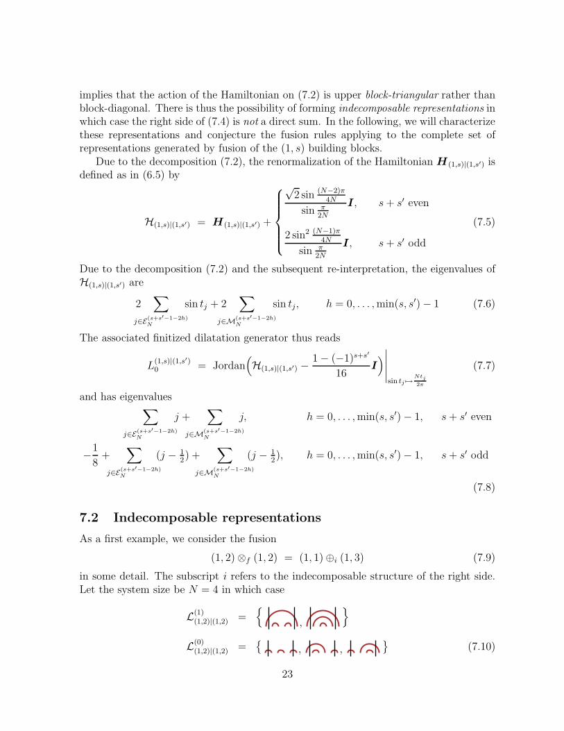
As a first example, we consider the fusion
(1, 2)⊗f (1, 2) = (1, 1)⊕i (1, 3) (7.9)
in some detail. The subscript i refers to the indecomposable structure of the right side.Let the system size be N = 4 in which case
L(1)(1,2)|(1,2) =
{
,
}
L(0)(1,2)|(1,2) =
{
, ,}
(7.10)
23
Acting on these link states listed in the order indicated here, the matrix representationof the Hamiltonian H(1,2)|(1,2) is
H(1,2)|(1,2) = −
0 2 0 1 11 0 0 0 00 0 0 1 10 0 1 0 00 0 1 0 0
(7.11)
The Jordan canonical form of the Hamiltonian H(1,2)|(1,2) thus reads
Jordan(
H(1,2)|(1,2)
)
= diag[
(
0 10 0
)
, 2 sinπ
4,
(
4 sin π4
10 4 sin π
4
)
]
(7.12)
in which case the finitized dilatation generator, after the replacement sin π47→ 4π
4
2π= 1
2,
becomes
L(1,2)|(1,2)0 = diag
[
(
0 10 0
)
, 1,
(
2 10 2
)
]
(7.13)
Also for N = 4, the finitized dilatation generators associated to H(1,1) and H(1,3) arelikewise found to be
L(1,1)0 = diag[0, 2], L
(1,3)0 = diag[0, 1, 2] (7.14)
This means that the finitized partition function associated to (7.11) decomposes as
Z(4)(1,2)|(1,2)(q) = χ
(4)(1,1)(q) + χ
(4)(1,3)(q) = q1/12[(1 + q2) + (1 + q + q2)]
= q1/12(2 + q + 2q2) (7.15)
in accordance with the fusion rule (7.9).The decomposition (7.15) does not contain information on the rank-two Jordan cells
appearing in (7.13) as the characters only reflect the diagonal part. The non-trivialJordan-cell structure is a finite-size manifestation of the right side of (7.9) being inde-
composable. It is observed that a Jordan cell is formed whenever possible and we haveverified for N = 2, 4, 6, 8 that this property persists. It is also noted that the Hamilto-nian is upper block-triangular meaning that states contributing to χ3(q) can be mappedto states contributing to χ1(q) but not vice versa. These observations are compatiblewith the properties of the indecomposable representation R1,1, appearing in [30], withcharacter χ1(q) + χ3(q). Assuming equivalence of the indecomposable representations,we will adopt their notation here and henceforth denote the right side of (7.9) by R1,1.
As a second example, we consider the fusion
(1, 2)⊗f (1, 4) = (1, 3)⊕i (1, 5) (7.16)
24
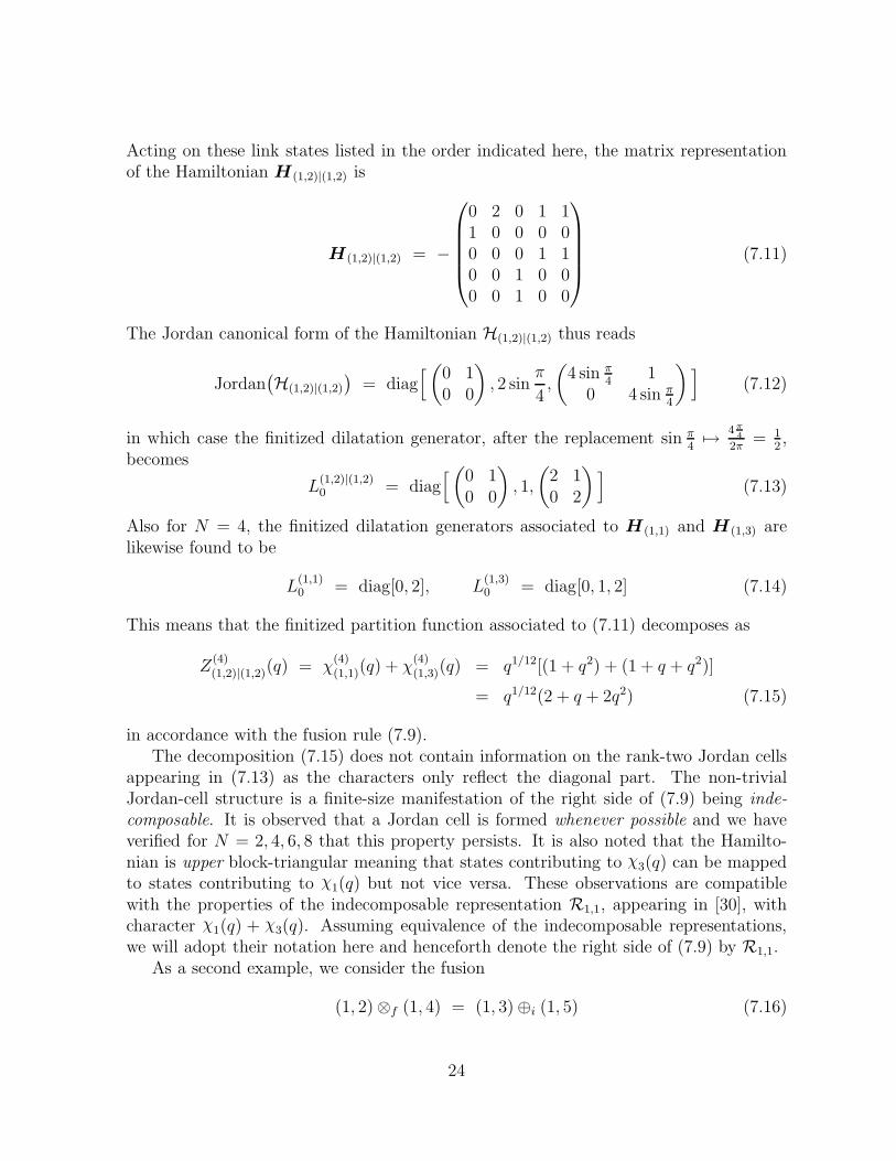
Let the system size be N = 6 in which case
L(1)(1,2)|(1,4) =
{
, , , ,
, , , ,
}
L(0)(1,2)|(1,4) =
{
, , , ,
}
(7.17)
Acting on these link states listed in the order indicated here, the matrix representationof the Hamiltonian H(1,2)|(1,4) is
H(1,2)|(1,4) = −
0
B
B
B
B
B
B
B
B
B
B
B
B
B
B
B
B
B
B
B
B
B
@
0 2 1 0 0 0 1 0 0 0 1 1 0 01 0 0 0 0 0 0 0 0 0 0 0 0 01 0 0 1 1 0 0 0 0 0 0 0 1 00 0 1 0 0 1 0 0 0 0 0 0 0 10 1 1 0 0 1 2 0 1 0 0 0 0 00 0 0 1 1 0 0 1 0 0 0 0 0 00 0 0 0 1 0 0 0 0 0 0 0 0 00 0 0 0 0 1 1 0 2 0 0 0 0 00 0 0 0 0 0 0 1 0 0 0 0 0 00 0 0 0 0 0 0 0 0 0 1 1 0 00 0 0 0 0 0 0 0 0 1 0 0 0 00 0 0 0 0 0 0 0 0 1 0 0 1 00 0 0 0 0 0 0 0 0 0 0 1 0 10 0 0 0 0 0 0 0 0 0 0 0 1 0
1
C
C
C
C
C
C
C
C
C
C
C
C
C
C
C
C
C
C
C
C
C
A
(7.18)
The Jordan canonical form of the associated renormalized Hamiltonian H(1,2)|(1,4) thusreads
Jordan(
H(1,2)|(1,4)
)
= diag[
0,
(
1 10 1
)
,
(√3 1
0√
3
)
, 2, 1 +√
3, 1 +√
3, 2√
3,
(
2 +√
3 1
0 2 +√
3
)
,
(
1 + 2√
3 1
0 1 + 2√
3
)
, 2 + 2√
3]
(7.19)
where we have used that 2 sin π6
= 1 and 2 sin π3
=√
3. The associated finitized dilatationgenerator is now found to be
L(1,2)|(1,4)0 = diag
[
0,
(
1 10 1
)
,
(
2 10 2
)
, 2, 3, 3, 4,
(
4 10 4
)
,
(
5 10 5
)
, 6]
(7.20)
It is observed that the repeated eigenvalue 3 does not form a Jordan cell. This is unlikethe fusion (7.9) above where a Jordan cell is formed whenever possible. Also for N = 6,the finitized dilatation generators associated to H(1,3) and H(1,5) are likewise found tobe
L(1,3)0 = diag[0, 1, 2, 2, 3, 4, 4, 5, 6], L
(1,5)0 = diag[1, 2, 3, 4, 5] (7.21)
25
This means that the finitized partition function associated to (7.18) decomposes as
Z(6)(1,2)|(1,4)(q) = χ
(6)(1,3)(q) + χ
(6)(1,5)(q)
= q1/12[(1 + q + 2q2 + q3 + 2q4 + q5 + q6) + q(1 + q + q2 + q3 + q4)]
= q1/12(1 + 2q + 3q2 + 2q3 + 3q4 + 2q5 + q6) (7.22)
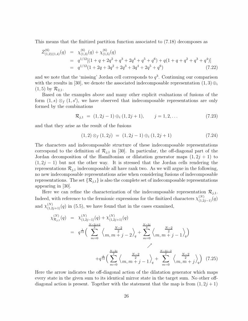
and we note that the ‘missing’ Jordan cell corresponds to q3. Continuing our comparisonwith the results in [30], we denote the associated indecomposable representation (1, 3)⊕i
(1, 5) by R2,1.Based on the examples above and many other explicit evaluations of fusions of the
form (1, s) ⊗f (1, s′), we have observed that indecomposable representations are onlyformed by the combinations
Rj,1 = (1, 2j − 1)⊕i (1, 2j + 1), j = 1, 2, . . . (7.23)
and that they arise as the result of the fusions
(1, 2)⊗f (1, 2j) = (1, 2j − 1)⊕i (1, 2j + 1) (7.24)
The characters and indecomposable structure of these indecomposable representationscorrespond to the definition of Rj,1 in [30]. In particular, the off-diagonal part of theJordan decomposition of the Hamiltonian or dilatation generator maps (1, 2j + 1) to(1, 2j − 1) but not the other way. It is stressed that the Jordan cells rendering therepresentations Rj,1 indecomposable all have rank two. As we will argue in the following,no new indecomposable representations arise when considering fusions of indecomposablerepresentations. The set {Rj,1} is also the complete set of indecomposable representationsappearing in [30].
Here we can refine the characterization of the indecomposable representation Rj,1.
Indeed, with reference to the fermionic expressions for the finitized characters χ(N)(1,2j−1)(q)
and χ(N)(1,2j+1)(q) in (5.5), we have found that in the cases examined,
χ(N)Rj,1
(q) = χ(N)(1,2j−1)(q) + χ(N)
(1,2j+1)(q)
= q112
(
N−2j+22
∑
m=0
⟨ N−22
m, m + j − 2
⟩
q+
N−2j
2∑
m=0
⟨ N−22
m, m + j − 1
⟩
q
)
ր
+q112
(
N−2j
2∑
m=0
⟨ N−22
m, m + j − 1
⟩
q+
N−2j−22
∑
m=0
⟨ N−22
m, m + j
⟩
q
)
(7.25)
Here the arrow indicates the off-diagonal action of the dilatation generator which mapsevery state in the given sum to its identical mirror state in the target sum. No other off-diagonal action is present. Together with the statement that the map is from (1, 2j + 1)
26
to (1, 2j − 1) only, this gives a full description of the indecomposable structure of (thefinitized version of) Rj,1. It is noted that the number of Jordan cells appearing in thefinitized version of Rj,1 is given by
limq→1
N−2j
2∑
m=0
⟨ N−22
m, m + j − 1
⟩
q=
(
N − 1N−2j
2
)
−(
N − 1N+2j
2
)
= limq→1
χ(N−1)1,2j (q) (7.26)
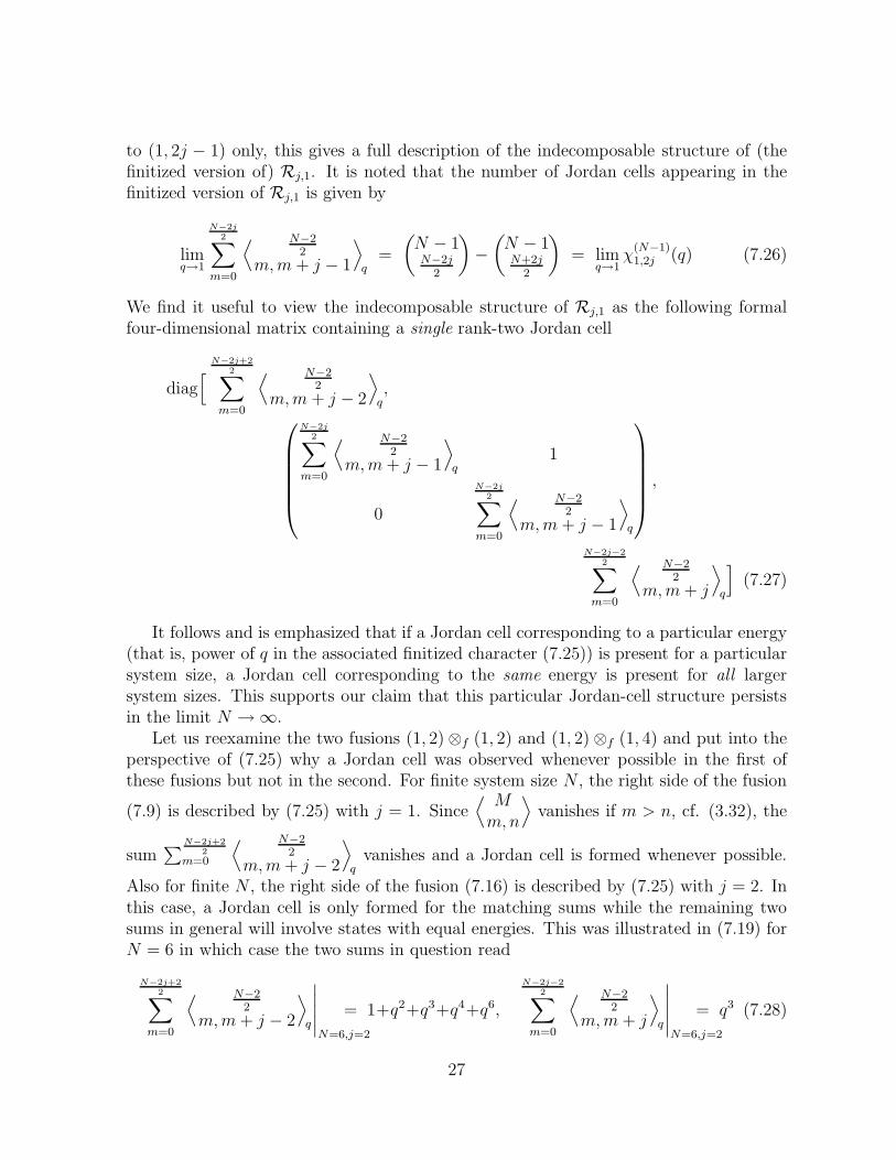
We find it useful to view the indecomposable structure of Rj,1 as the following formalfour-dimensional matrix containing a single rank-two Jordan cell
diag[
N−2j+22
∑
m=0
⟨ N−22
m, m + j − 2
⟩
q,
N−2j2
∑
m=0
⟨ N−22
m, m + j − 1
⟩
q1
0
N−2j2
∑
m=0
⟨ N−22
m, m + j − 1
⟩
q
,
N−2j−22
∑
m=0
⟨ N−22
m, m + j
⟩
q
]
(7.27)
It follows and is emphasized that if a Jordan cell corresponding to a particular energy(that is, power of q in the associated finitized character (7.25)) is present for a particularsystem size, a Jordan cell corresponding to the same energy is present for all largersystem sizes. This supports our claim that this particular Jordan-cell structure persistsin the limit N →∞.
Let us reexamine the two fusions (1, 2)⊗f (1, 2) and (1, 2)⊗f (1, 4) and put into theperspective of (7.25) why a Jordan cell was observed whenever possible in the first ofthese fusions but not in the second. For finite system size N , the right side of the fusion
(7.9) is described by (7.25) with j = 1. Since⟨ M
m, n
⟩
vanishes if m > n, cf. (3.32), the
sum∑
N−2j+22
m=0
⟨ N−22
m, m + j − 2
⟩
qvanishes and a Jordan cell is formed whenever possible.
Also for finite N , the right side of the fusion (7.16) is described by (7.25) with j = 2. Inthis case, a Jordan cell is only formed for the matching sums while the remaining twosums in general will involve states with equal energies. This was illustrated in (7.19) forN = 6 in which case the two sums in question read
N−2j+22
∑
m=0
⟨ N−22
m, m + j − 2
⟩
q
∣
∣
∣
∣
∣
N=6,j=2
= 1+q2+q3+q4+q6,
N−2j−22
∑
m=0
⟨ N−22
m, m + j
⟩
q
∣
∣
∣
∣
∣
N=6,j=2
= q3 (7.28)
27
This explains why the Jordan cell corresponding to q3 was ‘missing’.We wish to point out that one can be misled when considering very small system sizes
N . As this example illustrates
χ(2j−2)Rj,1
(q) = q12+∆1,2j−1 = χ
(2j−2)(1,2j−1)(q) (7.29)
an ambiguity due to finite-size effects can arise since the indecomposable structure ofRj,1 is only visible if N is big enough to accommodate it.
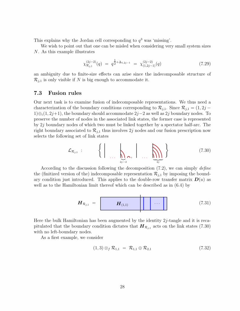
7.3 Fusion rules
Our next task is to examine fusion of indecomposable representations. We thus need acharacterization of the boundary conditions corresponding to Rj,1. Since Rj,1 = (1, 2j −1)⊕i(1, 2j+1), the boundary should accommodate 2j−2 as well as 2j boundary nodes. Topreserve the number of nodes in the associated link states, the former case is representedby 2j boundary nodes of which two must be linked together by a spectator half-arc. Theright boundary associated to Rj,1 thus involves 2j nodes and our fusion prescription nowselects the following set of link states
LRj,1:
{
,. . .|{z}
2j−2
. . .| {z }
2j
}
(7.30)
According to the discussion following the decomposition (7.2), we can simply define
the (finitized version of the) indecomposable representation Rj,1 by imposing the bound-ary condition just introduced. This applies to the double-row transfer matrix D(u) aswell as to the Hamiltonian limit thereof which can be described as in (6.4) by
HRj,1= H(1,1)
. . . (7.31)
Here the bulk Hamiltonian has been augmented by the identity 2j-tangle and it is reca-pitulated that the boundary condition dictates that HRj,1
acts on the link states (7.30)with no left-boundary nodes.
As a first example, we consider
(1, 3)⊗f R1,1 = R1,1 ⊕R2,1 (7.32)
28
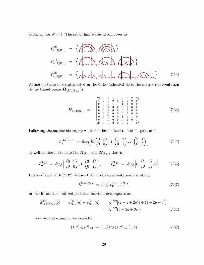
explicitly for N = 4. The set of link states decomposes as
L(2)(1,3)|R1,1
={
,
}
L(1)(1,3)|R1,1
={
, ,
}
L(0)(1,3)|R1,1
={
, , ,
}
(7.33)
Acting on these link states listed in the order indicated here, the matrix representationof the Hamiltonian H(1,3)|R1,1
is
H(1,3)|R1,1= −
0
B
B
B
B
B
B
B
B
B
B
B
@
0 2 0 1 1 0 0 0 01 0 0 0 0 0 0 0 00 0 0 1 1 1 0 0 00 0 1 0 0 0 0 0 00 0 1 0 0 0 0 0 00 0 0 0 0 0 0 0 00 0 0 0 0 1 0 1 00 0 0 0 0 0 1 0 10 0 0 0 0 0 0 1 0
1
C
C
C
C
C
C
C
C
C
C
C
A
(7.34)
Following the outline above, we work out the finitized dilatation generator
L(1,3)|R1,1
0 = diag[
0,
(
0 10 0
)
, 1,
(
1 10 1
)
, 2,
(
2 10 2
)
]
(7.35)
as well as those associated to HR1,1 and HR2,1 , that is,
LR1,1
0 = diag[
(
0 10 0
)
, 1,
(
2 10 2
)
]
, LR2,1
0 = diag[
0,
(
1 10 1
)
, 2]
(7.36)
In accordance with (7.32), we see that, up to a permutation operation,
L(1,3)|R1,1
0 = diag[LR1,1
0 , LR2,1
0 ] (7.37)
in which case the finitized partition function decomposes as
Z(4)(1,3)|R1,1
(q) = χ(4)R1,1
(q) + χ(4)R2,1
(q) = q1/12[(2 + q + 2q2) + (1 + 2q + q2)]
= q1/12(3 + 3q + 3q2) (7.38)
As a second example, we consider
(1, 2)⊗f R1,1 = (1, 2)⊕ (1, 2)⊕ (1, 4) (7.39)
29
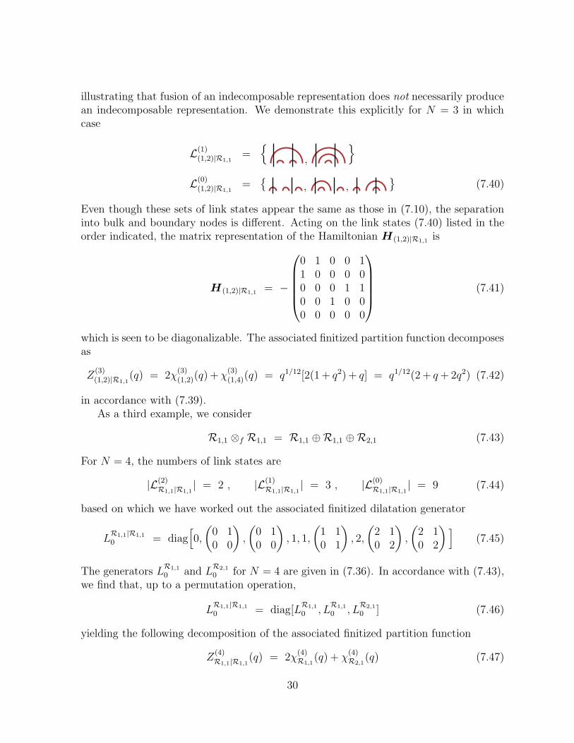
illustrating that fusion of an indecomposable representation does not necessarily producean indecomposable representation. We demonstrate this explicitly for N = 3 in whichcase
L(1)(1,2)|R1,1
={
,
}
L(0)(1,2)|R1,1
={
, ,}
(7.40)
Even though these sets of link states appear the same as those in (7.10), the separationinto bulk and boundary nodes is different. Acting on the link states (7.40) listed in theorder indicated, the matrix representation of the Hamiltonian H(1,2)|R1,1
is
H(1,2)|R1,1 = −
0 1 0 0 11 0 0 0 00 0 0 1 10 0 1 0 00 0 0 0 0
(7.41)
which is seen to be diagonalizable. The associated finitized partition function decomposesas
Z(3)(1,2)|R1,1
(q) = 2χ(3)(1,2)(q) + χ
(3)(1,4)(q) = q1/12[2(1 + q2) + q] = q1/12(2 + q + 2q2) (7.42)
in accordance with (7.39).As a third example, we consider
R1,1 ⊗f R1,1 = R1,1 ⊕R1,1 ⊕R2,1 (7.43)
For N = 4, the numbers of link states are
|L(2)R1,1|R1,1
| = 2 , |L(1)R1,1|R1,1
| = 3 , |L(0)R1,1|R1,1
| = 9 (7.44)
based on which we have worked out the associated finitized dilatation generator
LR1,1|R1,1
0 = diag[
0,
(
0 10 0
)
,
(
0 10 0
)
, 1, 1,
(
1 10 1
)
, 2,
(
2 10 2
)
,
(
2 10 2
)
]
(7.45)
The generators LR1,1
0 and LR2,1
0 for N = 4 are given in (7.36). In accordance with (7.43),we find that, up to a permutation operation,
LR1,1|R1,1
0 = diag[LR1,1
0 , LR1,1
0 , LR2,1
0 ] (7.46)
yielding the following decomposition of the associated finitized partition function
Z(4)R1,1|R1,1
(q) = 2χ(4)R1,1
(q) + χ(4)R2,1
(q) (7.47)
30
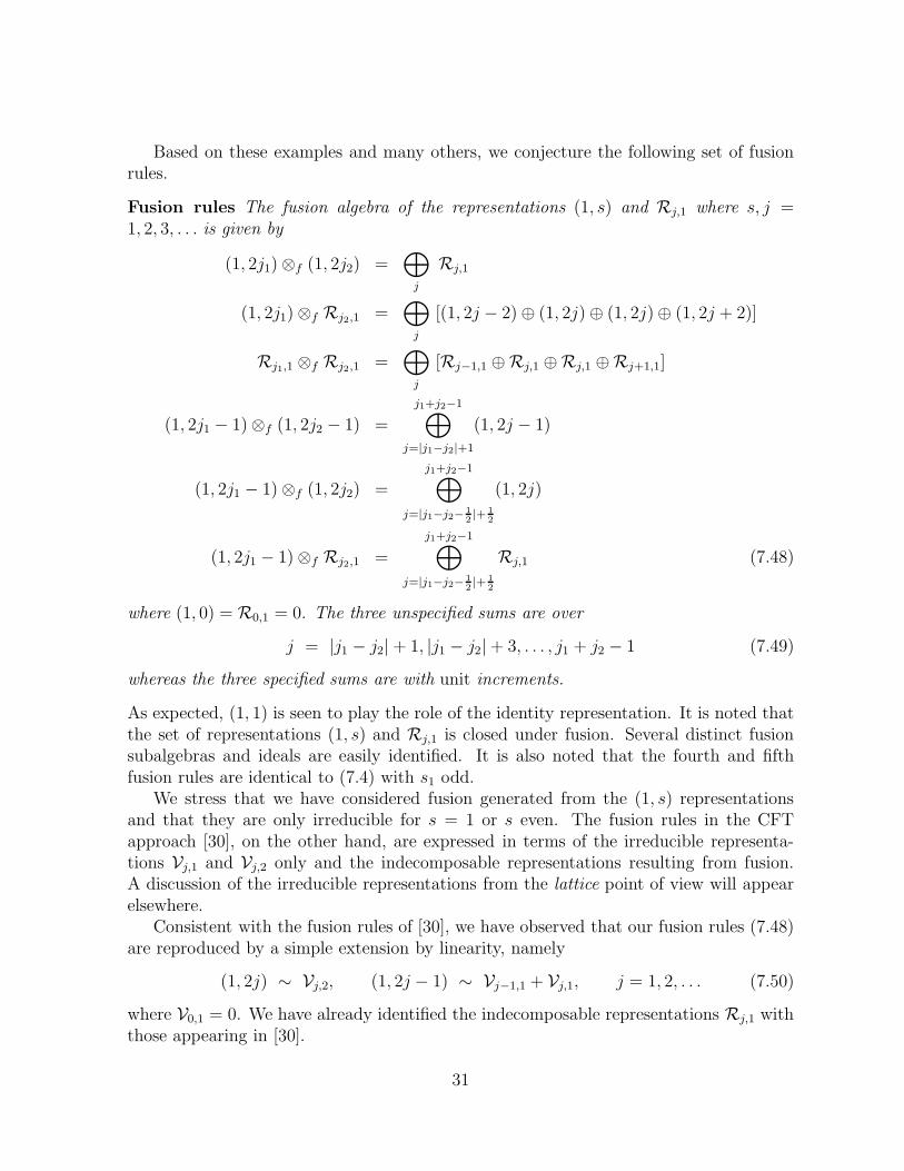
Based on these examples and many others, we conjecture the following set of fusionrules.
Fusion rules The fusion algebra of the representations (1, s) and Rj,1 where s, j =1, 2, 3, . . . is given by
(1, 2j1)⊗f (1, 2j2) =⊕
j
Rj,1
(1, 2j1)⊗f Rj2,1 =⊕
j
[(1, 2j − 2)⊕ (1, 2j)⊕ (1, 2j)⊕ (1, 2j + 2)]
Rj1,1 ⊗f Rj2,1 =⊕
j
[Rj−1,1 ⊕Rj,1 ⊕Rj,1 ⊕Rj+1,1]
(1, 2j1 − 1)⊗f (1, 2j2 − 1) =
j1+j2−1⊕
j=|j1−j2|+1
(1, 2j − 1)
(1, 2j1 − 1)⊗f (1, 2j2) =
j1+j2−1⊕
j=|j1−j2−12|+ 1
2
(1, 2j)
(1, 2j1 − 1)⊗f Rj2,1 =
j1+j2−1⊕
j=|j1−j2−12|+ 1
2
Rj,1 (7.48)
where (1, 0) = R0,1 = 0. The three unspecified sums are over
j = |j1 − j2|+ 1, |j1 − j2|+ 3, . . . , j1 + j2 − 1 (7.49)
whereas the three specified sums are with unit increments.
As expected, (1, 1) is seen to play the role of the identity representation. It is noted thatthe set of representations (1, s) and Rj,1 is closed under fusion. Several distinct fusionsubalgebras and ideals are easily identified. It is also noted that the fourth and fifthfusion rules are identical to (7.4) with s1 odd.
We stress that we have considered fusion generated from the (1, s) representationsand that they are only irreducible for s = 1 or s even. The fusion rules in the CFTapproach [30], on the other hand, are expressed in terms of the irreducible representa-tions Vj,1 and Vj,2 only and the indecomposable representations resulting from fusion.A discussion of the irreducible representations from the lattice point of view will appearelsewhere.
Consistent with the fusion rules of [30], we have observed that our fusion rules (7.48)are reproduced by a simple extension by linearity, namely
(1, 2j) ∼ Vj,2, (1, 2j − 1) ∼ Vj−1,1 + Vj,1, j = 1, 2, . . . (7.50)
where V0,1 = 0. We have already identified the indecomposable representations Rj,1 withthose appearing in [30].
31
8 Conclusion
In this paper, we have solved exactly a model of critical dense polymers on strips offinite width. This has been achieved, without invoking an n → 0 or Q → 0 limit,by solving directly our model of critical dense polymers within the framework of Yang-Baxter integrability. The calculations have been carried out for an infinite family of(1, s) integrable boundary conditions which impose ℓ = s − 1 defects in the bulk. Ourstudy of the physical combinatorics, which is the classification of the physical statesusing combinatorial objects, has revealed some interesting connections to q-Narayananumbers and natural generalizations thereof. Using the planar TL algebra, Yang-Baxtertechniques and functional equations in the form of inversion identities, we have been ableto calculate analytically the bulk and boundary free energies, the central charge c = −2,
the conformal weights ∆s = (2−s)2−18
and conformal characters in accord with previousresults [3, 4, 5, 6]. More particularly, since we were able to solve the model exactlyfor finite system sizes, we have explicitly confirmed the finitized conformal charactersproposed in [7].
In support of our claim that the CFT associated with critical dense polymers islogarithmic, we have shown in explicit examples how fusion of our (1, s) boundary con-ditions in some cases lead to indecomposable representations Rj,1. We have argued, byimplementing fusion diagrammatically, that fusion among the (1, s) representations andindecomposable representations Rj,1 closes, and we have conjectured the general form ofthe associated fusion rules. A proper comparison with the fusion algebra of Gaberdieland Kausch [30], however, requires that our fusion algebra is formulated in terms of ir-
reducible representations alongside the indecomposable representations. A discussion ofthese irreducible representations from the lattice point of view will appear elsewhere. Wehave nevertheless found that the fusion rules presented here are in accordance with thosein [30] in the sense that our fusion rules can be obtained from theirs by extending bylinearity to the (1, s) representations.
Again, it is a well-known abstract result [19] that the TL algebra admits indecom-posable representations at roots of unity. We emphasize that our motivation here is toconstruct explicit lattice Hamiltonians for these representations in the case of criticaldense polymers, to relate them to physical boundary conditions and to understand theirfusion properties in physical terms.
To claim a complete understanding of our model of critical dense polymers, we shouldstudy its extension from the strip to other topologies. Most importantly, the model shouldbe examined on the geometric cylinder and torus where the effects of non-contractibleloops will play a role. This constitutes work in progress.
Acknowledgments
This work is supported by the Australian Research Council. The authors thank Jean-Bernard Zuber for discussions.
32
References
[1] P.G. de Gennes, Phys. Rev. Lett. A38 (1972) 339; Scaling Concepts in Polymer
Physics, Cornell University, Ithaca (1979); J. des Cloizeaux, J. Phys. (Paris) 36
(1975) 281.
[2] C.M. Fortuin, P.W. Kasteleyn, Physica 57 (1972) 536; F.Y. Wu, Rev. Mod. Phys.54 (1982) 235.
[3] H. Saleur, J. Phys. A20 (1987) 455–470; J. Phys. A19 (1986) L807–L810; Phys.Rev. B35 (1987) 3657–3660.
[4] B. Duplantier, J. Phys. A19 (1986) L1009–L1014.
[5] H. Saleur, Nucl. Phys. B382 (1992) 486–531.
[6] N. Read, H. Saleur, Nucl. Phys. B613 (2001) 409.
[7] P.A. Pearce, J. Rasmussen, J.-B. Zuber, J. Stat. Mech. (2006) P11017.
[8] B. Duplantier, F. David, J. Stat. Phys. 51 (1988) 327–434.
[9] A. Sedrakyan, Nucl. Phys. B554 (1999) 514-536.
[10] M.R. Gaberdiel, H.G. Kausch, Phys. Lett. B386 (1996) 131–137.
[11] B.L. Feigin, A.M. Gainutdinov, A.M. Semikhatov, I.Yu. Tipunin, Nucl. Phys. B757
(2006) 303-343; Kazhdan-Lusztig dual quantum group for logarithmic extensions of
Virasoro models, hep-th/0606506 (2006).
[12] M.R. Gaberdiel, I. Runkel, J. Phys. A39 (2006) 14745-14780.
[13] H.G. Kausch, Nucl. Phys. B583 (2000) 513–541.
[14] S. Mahieu, P. Ruelle, Phys. Rev. E64 (2001) 066130; P. Ruelle, Phys. Lett. B539
(2002) 172–177; G. Piroux, P. Ruelle, J. Stat. Mech. 0410 (2004) P005; J. Phys.A38 (2005) 1451–1472; Phys. Lett. B607 (2005) 188–196.
[15] N.S. Izmailian, V.B. Priezzhev, P. Ruelle, C.-K. Hu, Phys. Rev. Lett. 95 (2005)260602.
[16] J.L. Jacobsen, N. Read, H. Saleur, Phys. Rev. Lett. 93 (2004) 038701.
[17] E.V. Ivashkevich, C.-K. Hu, Phys. Rev. E71 (2005) 015104 (R).
[18] V.F.R. Jones, Planar algebras I, math.QA/9909027.
33
[19] P.P. Martin, Potts models and related problems in statistical mechanics, Series onAdvances in Statistical Mechanics, Volume 5, World Scientific, Singapore (1991).
[20] J.L. Cardy, Nucl. Phys. B270 (1986) 186; Nucl. Phys. B275 (1986) 200; H. Saleur,M. Bauer, Nucl. Phys. B320 (1989) 591–624; J.L. Cardy, Nucl. Phys. B324 (1989)581–596; R.E. Behrend, P.A. Pearce, J.-B. Zuber, J. Phys. A31 (1998) L763-L770;R.E. Behrend, P.A. Pearce, V.B. Petkova, J.-B. Zuber, Nucl. Phys. B579 (2000)707-773; R.E. Behrend, P.A. Pearce, J. Stat. Phys. 102 (2001) 577–640.
[21] R.J. Baxter Exactly solved models in statistical mechanics (London, 1982) AcademicPress.
[22] D.L. O’Brien, P.A. Pearce, S.O. Warnaar, Physica A228 (1996) 63–77.
[23] R.E. Behrend, P.A. Pearce, D.L. O’Brien, J. Stat. Phys. 84 (1996) 1–48.
[24] P.A. Pearce, J. Rasmussen, Physical combinatorics of critical dense polymers, inpreparation (2006).
[25] J. Furlinger, J. Hofbauer, J. Combin. Theory A40 (1985) 248–264; P. Branden,Discrete Math. 281 (2004) 67–81.
[26] H.W.J. Blote, J.L. Cardy, M.P. Nightingale, Phys. Rev. Lett. 56 (1986) 742–745.
[27] I. Affleck, Phys. Rev. Lett. 56 (1986) 746-748.
[28] E. Melzer, Int. J. Mod. Phys. A9 (1994) 1115.
[29] A. Berkovich, Nucl. Phys. B431 (1994) 315.
[30] M.R. Gaberdiel, H.G. Kausch, Nucl. Phys. B477 (1996) 293–318.
34