Geometry on Non-Solvable Equations – A Survey

Linfan MAO

(Chinese Academy of Mathematics and System Science, Beijing 100190, P.R.China)

E-mail: maolinfan@163.com

Abstract: As we known, an objective thing not moves with one’s volition,

which implies that all contradictions, particularly, in these semiotic systems

for things are artificial. In classical view, a contradictory system is mean-

ingless, contrast to that of geometry on figures of things catched by eyes of

human beings. The main objective of sciences is holding the global behav-

ior of things, which needs one knowing both of compatible and contradictory

systems on things. Usually, a mathematical system included contradictions is

said to be a Smarandache system. Beginning from a famous fable, i.e., the

6 blind men with an elephant, this report shows the geometry on contradic-

tory systems, including non-solvable algebraic linear or homogenous equations,

non-solvable ordinary differential equations and non-solvable partial differen-

tial equations, classify such systems and characterize their global behaviors

by combinatorial geometry, particularly, the global stability of non-solvable

differential equations. Applications of such systems to other sciences, such as

those of gravitational fields, ecologically industrial systems can be also found

in this report. All of these discussions show that a non-solvable system is

nothing else but a system underlying a topological structure G 6≃ Kn with

a common intersection, i.e., mathematical combinatorics contrast to those of

solvable system underlying Kn, where n is the number of equations in this

system. However, if we stand on a geometrical viewpoint, they are compatible

and both of them are meaningful for human beings.

Key Words: Smarandache system, non-solvable system of equations, topo-

logical graph, GL-solution, global stability, ecologically industrial systems,

gravitational field, mathematical combinatorics.

AMS(2010): 03A10,05C15,20A05, 34A26,35A01,51A05,51D20,53A35

1Reported at the International Conference on Geometry and Its Applications, Jardpour Uni-

versity, October 16-18, 2014, Kolkata, India.

1

§1. Introduction

Loosely speaking, a geometry is mainly concerned with shape, size, position, · · ·etc., i.e., local or global characters of a figure in space. Its mainly objective is to

hold the global behavior of things. However, things are always complex, even hybrid

with other things. So it is difficult to know its global characters, or true face of a

thing sometimes.

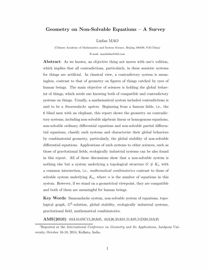
Let us consider a famous fable, i.e., the 6 blind men with an elephant following.

Fig.1

In this proverb, there are 6 blind men were asked to determine what an elephant

looked like by feeling different parts of the elephant’s body. The man touched the

elephant’s leg, tail, trunk, ear, belly or tusk respectively claims it’s like a pillar,

a rope, a tree branch, a hand fan, a wall or a solid pipe, such as those shown in

Fig.1 following. Each of them insisted on his own and not accepted others. They

then entered into an endless argument. All of you are right! A wise man explains

to them: why are you telling it differently is because each one of you touched the

different part of the elephant. So, actually the elephant has all those features what

you all said. Thus, the best result on an elephant for these blind men is

An elephant = 4 pillars⋃

1 rope⋃

1 tree branch⋃ 2 hand fans

⋃1 wall

⋃1 solid pipe,

i.e., a Smarandache multi-spaces ([23]-[25]) defined following.

2

Definition 1.1([12]-[13]) Let (Σ1;R1), (Σ2;R2), · · ·, (Σm;Rm) be m mathematical

systems, different two by two. A Smarandache multi-system Σ is a unionm⋃

i=1

Σi with

rules R =m⋃

i=1

Ri on Σ, denoted by(Σ; R

).

Then, what is the philosophical meaning of this fable for one understanding the

world? In fact, the situation for one realizing behaviors of things is analogous to

the blind men determining what an elephant looks like. Thus, this fable means the

limitation or unilateral of one’s knowledge, i.e., science because of all of those are

just correspondent with the sensory cognition of human beings.

Besides, we know that contradiction exists everywhere by this fable, which

comes from the limitation of unilateral sensory cognition, i.e., artificial contradiction

of human beings, and all scientific conclusions are nothing else but an approximation

for things. For example, let µ1, µ2, · · · , µn be known and νi, i ≥ 1 unknown characters

at time t for a thing T . Then, the thing T should be understood by

T =

(n⋃

i=1

µi)⋃(⋃

k≥1

νk)

in logic but with an approximation T =n⋃

i=1

µi for T by human being at time t.

Even for T , these are maybe contradictions in characters µ1, µ2, · · · , µn with endless

argument between researchers, such as those implied in the fable of 6 blind men with

an elephant. Consequently, if one stands still on systems without contradictions, he

will never hold the real face of things in the world, particularly, the true essence of

geometry for limited of his time.

However, all things are inherently related, not isolated in philosophy, i.e., under-

lying an invariant topological structure G ([4],[22]). Thus, one needs to characterize

those things on contradictory systems, particularly, by geometry. The main objec-

tive of this report is to discuss the geometry on contradictory systems, including

non-solvable algebraic equations, non-solvable ordinary or partial differential equa-

tions, classify such systems and characterize their global behaviors by combinatorial

geometry, particularly, the global stability of non-solvable differential equations. For

terminologies and notations not mentioned here, we follow references [11], [13] for

topological graphs, [3]-[4] for topology, [12],[23]-[25] for Smarandache multi-spaces

and [2],[26] for partial or ordinary differential equations.

3

§2. Manifolds on Equation Systems

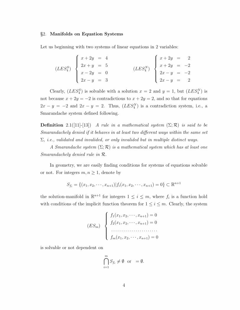
Let us beginning with two systems of linear equations in 2 variables:

(LESS4 )

x + 2y = 4

2x + y = 5

x − 2y = 0

2x − y = 3

(LESN4 )

x + 2y = 2

x + 2y = −2

2x − y = −2

2x − y = 2

Clearly, (LESS4 ) is solvable with a solution x = 2 and y = 1, but (LESN

4 ) is

not because x + 2y = −2 is contradictious to x + 2y = 2, and so that for equations

2x − y = −2 and 2x − y = 2. Thus, (LESN4 ) is a contradiction system, i.e., a

Smarandache system defined following.

Definition 2.1([11]-[13]) A rule in a mathematical system (Σ;R) is said to be

Smarandachely denied if it behaves in at least two different ways within the same set

Σ, i.e., validated and invalided, or only invalided but in multiple distinct ways.

A Smarandache system (Σ;R) is a mathematical system which has at least one

Smarandachely denied rule in R.

In geometry, we are easily finding conditions for systems of equations solvable

or not. For integers m, n ≥ 1, denote by

Sfi= (x1, x2, · · · , xn+1)|fi(x1, x2, · · · , xn+1) = 0 ⊂ R

n+1

the solution-manifold in Rn+1 for integers 1 ≤ i ≤ m, where fi is a function hold

with conditions of the implicit function theorem for 1 ≤ i ≤ m. Clearly, the system

(ESm)

f1(x1, x2, · · · , xn+1) = 0

f2(x1, x2, · · · , xn+1) = 0

. . . . . . . . . . . . . . . . . . . . . . .

fm(x1, x2, · · · , xn+1) = 0

is solvable or not dependent on

m⋂

i=1

Sfi6= ∅ or = ∅.

4

Conversely, if D is a geometrical space consisting of m manifolds D1, D2, · · · , Dm

in Rn+1, where,

Di = (x1, x2, · · · , xn+1)|f [i]k (x1, x2, · · · , xn+1) = 0, 1 ≤ k ≤ mi =

mi⋂

k=1

Sf[i]k

.

Then, the system

f[i]1 (x1, x2, · · · , xn+1) = 0

f[i]2 (x1, x2, · · · , xn+1) = 0

. . . . . . . . . . . . . . . . . . . . . . . .

f[i]mi(x1, x2, · · · , xn+1) = 0

1 ≤ i ≤ m

is solvable or not dependent on the intersection

m⋂

i=1

Di 6= ∅ or = ∅.

Thus, we obtain the following result.

Theorem 2.2 If a geometrical space D consists of m parts D1, D2, · · · , Dm, where,

Di = (x1, x2, · · · , xn+1)|f [i]k (x1, x2, · · · , xn+1) = 0, 1 ≤ k ≤ mi, then the system

(ESm) consisting of

f[i]1 (x1, x2, · · · , xn+1) = 0

f[i]2 (x1, x2, · · · , xn+1) = 0

. . . . . . . . . . . . . . . . . . . . . . .

f[i]mi(x1, x2, · · · , xn+1) = 0

1 ≤ i ≤ m

is non-solvable if

m⋂

i=1

Di = ∅.

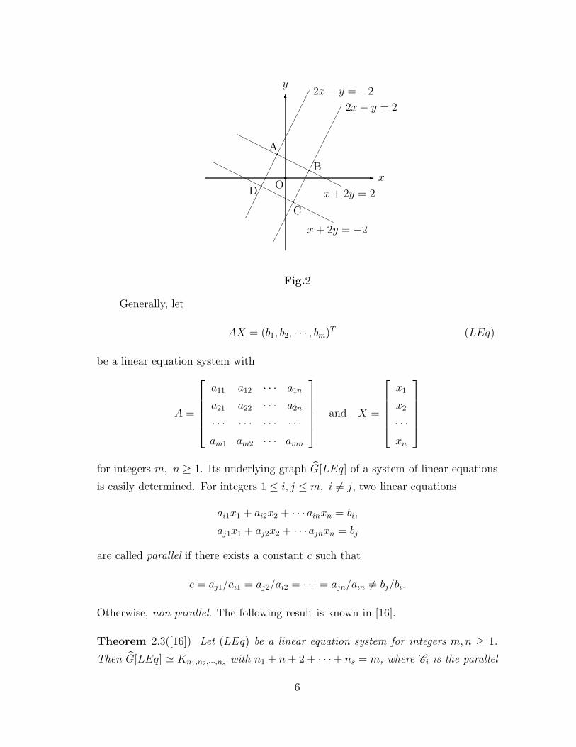
Now, whether is it meaningless for a contradiction system in the world? Cer-

tainly not! As we discussed in the last section, a contradiction is artificial if such

a system indeed exists in the world. The objective for human beings is not just

finding contradictions, but holds behaviors of such systems. For example, although

the system (LESN4 ) is contradictory, but it really exists, i.e., 4 lines in R2, such as

those shown in Fig.2.

5

-6

Ox

y

x + 2y = 2

x + 2y = −2

2x − y = −2

2x − y = 2

A

B

C

D

Fig.2

Generally, let

AX = (b1, b2, · · · , bm)T (LEq)

be a linear equation system with

A =

a11 a12 · · · a1n

a21 a22 · · · a2n

· · · · · · · · · · · ·am1 am2 · · · amn

and X =

x1

x2

· · ·xn

for integers m, n ≥ 1. Its underlying graph G[LEq] of a system of linear equations

is easily determined. For integers 1 ≤ i, j ≤ m, i 6= j, two linear equations

ai1x1 + ai2x2 + · · ·ainxn = bi,

aj1x1 + aj2x2 + · · ·ajnxn = bj

are called parallel if there exists a constant c such that

c = aj1/ai1 = aj2/ai2 = · · · = ajn/ain 6= bj/bi.

Otherwise, non-parallel. The following result is known in [16].

Theorem 2.3([16]) Let (LEq) be a linear equation system for integers m, n ≥ 1.

Then G[LEq] ≃ Kn1,n2,···,nswith n1 + n + 2 + · · ·+ ns = m, where Ci is the parallel

6

family by the property that all equations in a family Ci are parallel and there are no

other equations parallel to lines in Ci for integers 1 ≤ i ≤ s, ni = |Ci| for integers

1 ≤ i ≤ s in (LEq) and (LEq) is non-solvable if s ≥ 2.

Particularly, for linear equation system on 2 variables, let H be a planar graph

with edges straight segments on R2. The c-line graph LC(H) on H is defined by

V (LC(H)) = straight lines L = e1e2 · · · el, s ≥ 1 in H;E(LC(H)) = (L1, L2)| L1 = e1

1e12 · · · e1

l , L2 = e21e

22 · · · e2

s, l, s ≥ 1

and there adjacent edges e1i , e2

j in H, 1 ≤ i ≤ l, 1 ≤ j ≤ s.

Then, a simple criterion in [16] following is interesting.

Theorem 2.4([16]) A linear equation system (LEq2) on 2 variables is non-solvable

if and only if G[LEq2] ≃ LC(H)), where H is a planar graph of order |H| ≥ 2 on

R2 with each edge a straight segment

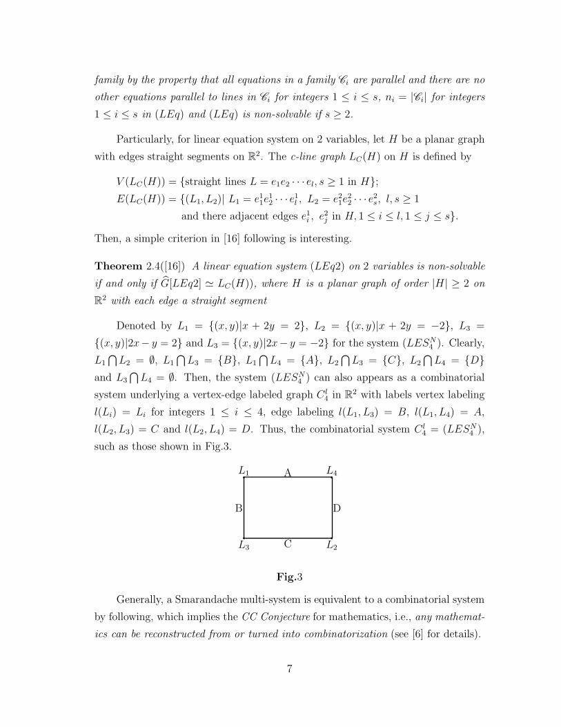
Denoted by L1 = (x, y)|x + 2y = 2, L2 = (x, y)|x + 2y = −2, L3 =

(x, y)|2x− y = 2 and L3 = (x, y)|2x− y = −2 for the system (LESN4 ). Clearly,

L1

⋂L2 = ∅, L1

⋂L3 = B, L1

⋂L4 = A, L2

⋂L3 = C, L2

⋂L4 = D

and L3

⋂L4 = ∅. Then, the system (LESN

4 ) can also appears as a combinatorial

system underlying a vertex-edge labeled graph C l4 in R2 with labels vertex labeling

l(Li) = Li for integers 1 ≤ i ≤ 4, edge labeling l(L1, L3) = B, l(L1, L4) = A,

l(L2, L3) = C and l(L2, L4) = D. Thus, the combinatorial system C l4 = (LESN

4 ),

such as those shown in Fig.3.

L1

L2L3

L4A

B

C

D

Fig.3

Generally, a Smarandache multi-system is equivalent to a combinatorial system

by following, which implies the CC Conjecture for mathematics, i.e., any mathemat-

ics can be reconstructed from or turned into combinatorization (see [6] for details).

7

Definition 2.5([11]-[13]) For any integer m ≥ 1, let(Σ; R

)be a Smarandache

multi-system consisting of m mathematical systems (Σ1;R1), (Σ2;R2), · · ·, (Σm;Rm).

An inherited topological structure GL[S]

of(Σ; R

)is a topological vertex-edge la-

beled graph defined following:

V(GL[S])

= Σ1, Σ2, · · · , Σm,

E(GL[S])

= (Σi, Σj) |Σi

⋂Σj 6= ∅, 1 ≤ i 6= j ≤ m with labeling

L : Σi → L (Σi) = Σi and L : (Σi, Σj) → L (Σi, Σj) = Σi

⋂Σj

for integers 1 ≤ i 6= j ≤ m.

Thus, a Smarandache system is equivalent to a combinatorial system, i.e.,(Σ; R

)≃ GL

[S]

underlying with a graph G[S]

without labels. Particularly, let

these mathematical systems (Σ1;R1), (Σ2;R2), · · ·, (Σm;Rm) be geometrical spaces,

for instance manifolds M1, M2, · · · , Mm with respective dimensions n1, n2, · · · , nm in

Definition 2.3, we get a geometrical space with M =m⋃

i=1

Mi underlying a topological

graph GL[M]. Such a geometrical space GL

[M]

is called a combinatorial manifold,

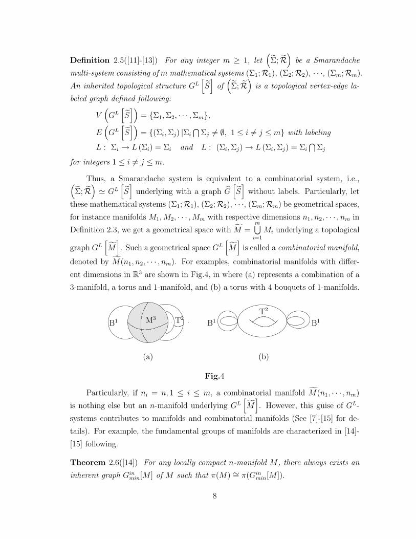
denoted by M(n1, n2, · · · , nm). For examples, combinatorial manifolds with differ-

ent dimensions in R3 are shown in Fig.4, in where (a) represents a combination of a

3-manifold, a torus and 1-manifold, and (b) a torus with 4 bouquets of 1-manifolds.

M3B1 T2

(a)

T2

B1 B1

(b)

Fig.4

Particularly, if ni = n, 1 ≤ i ≤ m, a combinatorial manifold M(n1, · · · , nm)

is nothing else but an n-manifold underlying GL[M]. However, this guise of GL-

systems contributes to manifolds and combinatorial manifolds (See [7]-[15] for de-

tails). For example, the fundamental groups of manifolds are characterized in [14]-

[15] following.

Theorem 2.6([14]) For any locally compact n-manifold M , there always exists an

inherent graph Ginmin[M ] of M such that π(M) ∼= π(Gin

min[M ]).

8

Particularly, for an integer n ≥ 2 a compact n-manifold M is simply-connected

if and only if Ginmin[M ] is a finite tree.

Theorem 2.7([15]) Let M be a finitely combinatorial manifold. If for ∀(M1, M2) ∈E(GL

[M]), M1 ∩ M2 is simply-connected, then

π1(M) ∼=

⊕

M∈V (G[M ])

π1(M)

⊕π1(G

[M]).

Furthermore, it provides one with a listing of manifolds by graphs in [14].

Theorem 2.8([14]) Let A [M ] = (Uλ; ϕλ) | λ ∈ Λ be a atlas of a locally compact

n-manifold M . Then the labeled graph GL|Λ| of M is a topological invariant on |Λ|,

i.e., if HL1

|Λ| and GL2

|Λ| are two labeled n-dimensional graphs of M , then there exists

a self-homeomorphism h : M → M such that h : HL1

|Λ| → GL2

|Λ| naturally induces an

isomorphism of graph.

Why the system (ESm) consisting of

f[i]1 (x1, x2, · · · , xn) = 0

f[i]2 (x1, x2, · · · , xn) = 0

. . . . . . . . . . . . . . . . . . . . . .

f[i]mi(x1, x2, · · · , xn) = 0

1 ≤ i ≤ m

is non-solvable ifm⋂

i=1

Di = ∅ in Theorem 2.2? In fact, it lies in that the solution-

manifold of (ESm) is the intersection of Di, 1 ≤ i ≤ m. If it is allowed combinatorial

manifolds to be solution-manifolds, then there are no contradictions once more even

ifm⋂

i=1

Di = ∅. This fact implies that including combinatorial manifolds to be solution-

manifolds of systems (ESm) is a better understanding things in the world.

§3. Surfaces on Homogenous Polynomials

Let

P1(x), P2(x), · · · , Pm(x) (ESn+1m )

be m homogeneous polynomials in variables x1, x2, · · · , xn+1 with coefficients in C

and

∅ 6= SPi= (x1, x2, · · · , xn+1)|Pi (x) = 0 ⊂ P

nC

9

for integers 1 ≤ i ≤ m, which are hypersurfaces, particularly, curves if n = 2 passing

through the original of Cn+1.

Similarly, parallel hypersurfaces in Cn+1 are defined following.

Definition 3.1 Let P (x), Q(x) be two complex homogenous polynomials of degree

d in n + 1 variables and I(P, Q) the set of intersection points of P (x) with Q(x).

They are said to be parallel, denoted by P ‖ Q if d ≥ 1 and there are constants

a, b, · · · , c (not all zero) such that for ∀x ∈ I(P, Q), ax1 + bx2 + · · ·+ cxn+1 = 0, i.e.,

all intersections of P (x) with Q(x) appear at a hyperplane on PnC, or d = 1 with

all intersections at the infinite xn+1 = 0. Otherwise, P (x) are not parallel to Q(x),

denoted by P 6‖ Q.

Then, these polynomials in (ESn+1m ) can be classified into families C1, C2, · · · , Cl

by this parallel property such that Pi ‖ Pj if Pi, Pj ∈ Ck for an integer 1 ≤ k ≤ l,

where 1 ≤ i 6= j ≤ mand it is maximal if each Ci is maximal for integers 1 ≤ i ≤ l,

i.e., for ∀P ∈ Pk(x), 1 ≤ k ≤ m\Ci, there is a polynomial Q(x) ∈ Ci such that

P 6‖ Q. The following result is a generalization of Theorem 2.3.

Theorem 3.2([19]) Let n ≥ 2 be an integer. For a system (ESn+1m ) of homogenous

polynomials with a parallel maximal classification C1, C2, · · · , Cl,

G[ESn+1m ] ≤ K(C1, C2, · · · , Cl)

and with equality holds if and only if Pi ‖ Pj and Ps 6‖ Pi implies that Ps 6‖ Pj, where

K(C1, C2, · · · , Cl) denotes a complete l-partite graphs. Conversely, for any subgraph

G ≤ K(C1, C2, · · · , Cl), there are systems (ESn+1m ) of homogenous polynomials with

a parallel maximal classification C1, C2, · · · , Cl such that

G ≃ G[ESn+1m ].

Particularly, if all polynomials in (ESn+1m ) be degree 1, i.e., hyperplanes with a

parallel maximal classification C1, C2, · · · , Cl, then

G[ESn+1m ] = K(C1, C2, · · · , Cl).

The following result is immediately known by definition.

10

Theorem 3.3 Let (ESn+1m ) be a GL-system consisting of homogenous polynomials

P (x1), P (x2), · · · , P (xm) in n + 1 variables with respectively hypersurfaces SPi, 1 ≤

i ≤ m. Then, M =m⋃

i=1

SPiis an n-manifold underlying graph G[ESn+1

m ] in Cn+1.

For n = 2, we can further determine the genus of surface M in R3 following.

Theorem 3.4([19]) Let S be a combinatorial surface consisting of m orientable

surfaces S1, S2, · · · , Sm underlying a topological graph GL[S] in R3. Then

g(S) = β(G⟨S⟩) +

m∑

i=1

(−1)i+1∑

i⋂l=1

Skl6=∅

[g

(i⋂

l=1

Skl

)− c

(i⋂

l=1

Skl

)+ 1

],

where g

(i⋂

l=1

Skl

), c

(i⋂

l=1

Skl

)are respectively the genus and number of path-connected

components in surface Sk1

⋂Sk2

⋂ · · ·⋂Skiand β(G

⟨S⟩) denotes the Betti number

of topological graph G⟨S⟩.

Notice that for a curve C determined by homogenous polynomial P (x, y, z) of

degree d in P2C, there is a compact connected Riemann surface S by the Noether’s

result such that

h : S − h−1(Sing(C)) → C − Sing(C)

is a homeomorphism with genus

g(S) =1

2(d − 1)(d − 2) −

∑

p∈Sing(C)

δ(p),

where δ(p) is a positive integer associated with the singular point p in C. Further-

more, if Sing(C) = ∅, i.e., C is non-singular then there is a compact connected

Riemann surface S homeomorphism to C with genus1

2(d− 1)(d− 2). By Theorem

3.4, we obtain the genus of S determined by homogenous polynomials following.

Theorem 3.5([19]) Let C1, C2, · · · , Cm be complex curves determined by homogenous

polynomials P1(x, y, z), P2(x, y, z), · · · , Pm(x, y, z) without common component, and

let

RPi,Pj=

deg(Pi)deg(Pj)∏

k=1

(cijk z − bij

k y)eijk , ωi,j =

deg(Pi)deg(Pj)∑

k=1

∑

eijk6=0

1

11

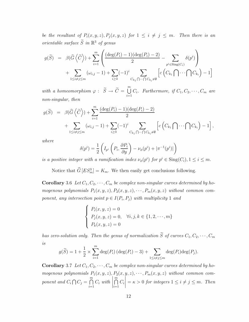
be the resultant of Pi(x, y, z), Pj(x, y, z) for 1 ≤ i 6= j ≤ m. Then there is an

orientable surface S in R3 of genus

g(S) = β(G⟨C⟩) +

m∑

i=1

(deg(Pi) − 1)(deg(Pi) − 2)

2−

∑

pi∈Sing(Ci)

δ(pi)

+∑

1≤i6=j≤m

(ωi,j − 1) +∑

i≥3

(−1)i∑

Ck1

⋂···⋂

Cki6=∅

[c(Ck1

⋂· · ·⋂

Cki

)− 1]

with a homeomorphism ϕ : S → C =m⋃

i=1

Ci. Furthermore, if C1, C2, · · · , Cm are

non-singular, then

g(S) = β(G⟨C⟩) +

m∑

i=1

(deg(Pi) − 1)(deg(Pi) − 2)

2

+∑

1≤i6=j≤m

(ωi,j − 1) +∑

i≥3

(−1)i∑

Ck1

⋂···⋂

Cki6=∅

[c(Ck1

⋂· · ·⋂

Cki

)− 1],

where

δ(pi) =1

2

(Ipi

(Pi,

∂Pi

∂y

)− νφ(p

i) + |π−1(pi)|)

is a positive integer with a ramification index νφ(pi) for pi ∈ Sing(Ci), 1 ≤ i ≤ m.

Notice that G [ES3m] = Km. We then easily get conclusions following.

Corollary 3.6 Let C1, C2, · · · , Cm be complex non-singular curves determined by ho-

mogenous polynomials P1(x, y, z), P2(x, y, z), · · · , Pm(x, y, z) without common com-

ponent, any intersection point p ∈ I(Pi, Pj) with multiplicity 1 and

Pi(x, y, z) = 0

Pj(x, y, z) = 0,

Pk(x, y, z) = 0

∀i, j, k ∈ 1, 2, · · · , m

has zero-solution only. Then the genus of normalization S of curves C1, C2, · · · , Cm

is

g(S) = 1 +1

2×

m∑

i=1

deg(Pi) (deg(Pi) − 3) +∑

1≤i6=j≤m

deg(Pi)deg(Pj).

Corollary 3.7 Let C1, C2, · · · , Cm be complex non-singular curves determined by ho-

mogenous polynomials P1(x, y, z), P2(x, y, z), · · · , Pm(x, y, z) without common com-

ponent and Ci

⋂Cj =

m⋂i=1

Ci with

∣∣∣∣m⋂

i=1

Ci

∣∣∣∣ = κ > 0 for integers 1 ≤ i 6= j ≤ m. Then

12

the genus of normalization S of curves C1, C2, · · · , Cm is

g(S) = g(S) = (κ − 1)(m − 1) +m∑

i=1

(deg(Pi) − 1)(deg(Pi) − 2)

2.

Particularly, if all curves in C3 are lines, we know an interesting result following.

Corollary 3.8 Let L1, L2, · · · , Lm be distinct lines in P2C with respective normal-

izations of spheres S1, S2, · · · , Sm. Then there is a normalization of surface S of

L1, L2, · · · , Lm with genus β(G⟨L⟩). Particularly, if G

⟨L⟩) is a tree, then S is

homeomorphic to a sphere.

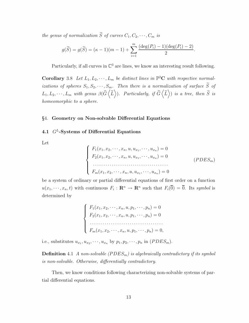
§4. Geometry on Non-solvable Differential Equations

4.1 GL-Systems of Differential Equations

Let

F1(x1, x2, · · · , xn, u, ux1, · · · , uxn) = 0

F2(x1, x2, · · · , xn, u, ux1, · · · , uxn) = 0

. . . . . . . . . . . . . . . . . . . . . . . . . . . . . . . . . . . .

Fm(x1, x2, · · · , xn, u, ux1, · · · , uxn) = 0

(PDESm)

be a system of ordinary or partial differential equations of first order on a function

u(x1, · · · , xn, t) with continuous Fi : Rn → Rn such that Fi(0) = 0. Its symbol is

determined by

F1(x1, x2, · · · , xn, u, p1, · · · , pn) = 0

F2(x1, x2, · · · , xn, u, p1, · · · , pn) = 0

. . . . . . . . . . . . . . . . . . . . . . . . . . . . . . . . . . .

Fm(x1, x2, · · · , xn, u, p1, · · · , pn) = 0,

i.e., substitutes ux1, ux2, · · · , uxnby p1, p2, · · · , pn in (PDESm).

Definition 4.1 A non-solvable (PDESm) is algebraically contradictory if its symbol

is non-solvable. Otherwise, differentially contradictory.

Then, we know conditions following characterizing non-solvable systems of par-

tial differential equations.

13

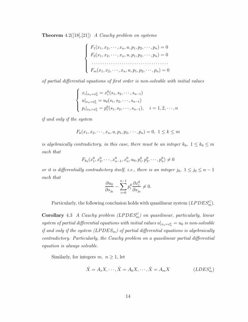
Theorem 4.2([18],[21]) A Cauchy problem on systems

F1(x1, x2, · · · , xn, u, p1, p2, · · · , pn) = 0

F2(x1, x2, · · · , xn, u, p1, p2, · · · , pn) = 0

. . . . . . . . . . . . . . . . . . . . . . . . . . . . . . . . . . . .

Fm(x1, x2, · · · , xn, u, p1, p2, · · · , pn) = 0

of partial differential equations of first order is non-solvable with initial values

xi|xn=x0n

= x0i (s1, s2, · · · , sn−1)

u|xn=x0n

= u0(s1, s2, · · · , sn−1)

pi|xn=x0n

= p0i (s1, s2, · · · , sn−1), i = 1, 2, · · · , n

if and only if the system

Fk(x1, x2, · · · , xn, u, p1, p2, · · · , pn) = 0, 1 ≤ k ≤ m

is algebraically contradictory, in this case, there must be an integer k0, 1 ≤ k0 ≤ m

such that

Fk0(x01, x

02, · · · , x0

n−1, x0n, u0, p

01, p

02, · · · , p0

n) 6= 0

or it is differentially contradictory itself, i.e., there is an integer j0, 1 ≤ j0 ≤ n − 1

such that∂u0

∂sj0

−n−1∑

i=0

p0i

∂x0i

∂sj0

6= 0.

Particularly, the following conclusion holds with quasilinear system (LPDESCm).

Corollary 4.3 A Cauchy problem (LPDESCm) on quasilinear, particularly, linear

system of partial differential equations with initial values u|xn=x0n

= u0 is non-solvable

if and only if the system (LPDESm) of partial differential equations is algebraically

contradictory. Particularly, the Cauchy problem on a quasilinear partial differential

equation is always solvable.

Similarly, for integers m, n ≥ 1, let

X = A1X, · · · , X = AkX, · · · , X = AmX (LDES1m)

14

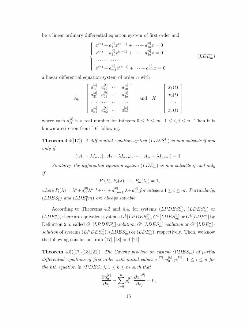
be a linear ordinary differential equation system of first order and

x(n) + a[0]11x

(n−1) + · · ·+ a[0]1nx = 0

x(n) + a[0]21x

(n−1) + · · ·+ a[0]2nx = 0

· · · · · · · · · · · ·x(n) + a

[0]m1x

(n−1) + · · · + a[0]mnx = 0

(LDEnm)

a linear differential equation system of order n with

Ak =

a[k]11 a

[k]12 · · · a

[k]1n

a[k]21 a

[k]22 · · · a

[k]2n

· · · · · · · · · · · ·a

[k]n1 a

[k]n2 · · · a

[k]nn

and X =

x1(t)

x2(t)

· · ·xn(t)

where each a[k]ij is a real number for integers 0 ≤ k ≤ m, 1 ≤ i, j ≤ n. Then it is

known a criterion from [16] following.

Theorem 4.4([17]) A differential equation system (LDES1m) is non-solvable if and

only if

(|A1 − λIn×n|, |A2 − λIn×n|, · · · , |Am − λIn×n|) = 1.

Similarly, the differential equation system (LDEnm) is non-solvable if and only

if

(P1(λ), P2(λ), · · · , Pm(λ)) = 1,

where Pi(λ) = λn+a[0]i1 λn−1+· · ·+a

[0]i(n−1)λ+a

[0]in for integers 1 ≤ i ≤ m. Particularly,

(LDES11) and (LDEn

1 m) are always solvable.

According to Theorems 4.3 and 4.4, for systems (LPDESCm), (LDES1

m) or

(LDEnm), there are equivalent systems GL[LPDESC

m], GL[LDES1m] or GL[LDEn

m] by

Definition 2.5, called GL[LPDESCm]-solution, GL[LDES1

m] -solution or GL[LDEnm]-

solution of systems (LPDESCm), (LDES1

m) or (LDEnm), respectively. Then, we know

the following conclusion from [17]-[18] and [21].

Theorem 4.5([17]-[18],[21]) The Cauchy problem on system (PDESm) of partial

differential equations of first order with initial values x[k0]i , u

[k]0 , p

[k0]i , 1 ≤ i ≤ n for

the kth equation in (PDESm), 1 ≤ k ≤ m such that

∂u[k]0

∂sj

−n∑

i=0

p[k0]i

∂x[k0]i

∂sj

= 0,

15

and the linear homogeneous differential equation system (LDES1m) (or (LDEn

m))

both are uniquely GL-solvable, i.e., GL[PDES], GL[LDES1m] and GL[LDEn

m] are

uniquely determined.

For ordinary differential systems (LDES1m) or (LDEn

m), we can further replace

solution-manifolds S [k] of the kth equation in GL[LDES1m] and GL[LDEn

m] by their

solution basis

B[k] = β

[k]

i (t)eα[k]i t | 1 ≤ i ≤ n or C

[k] = tleλ[k]i t | 1 ≤ i ≤ s, 1 ≤ l ≤ ki .

because each solution-manifold of (LDES1m) (or (LDEn

m)) is a linear space.

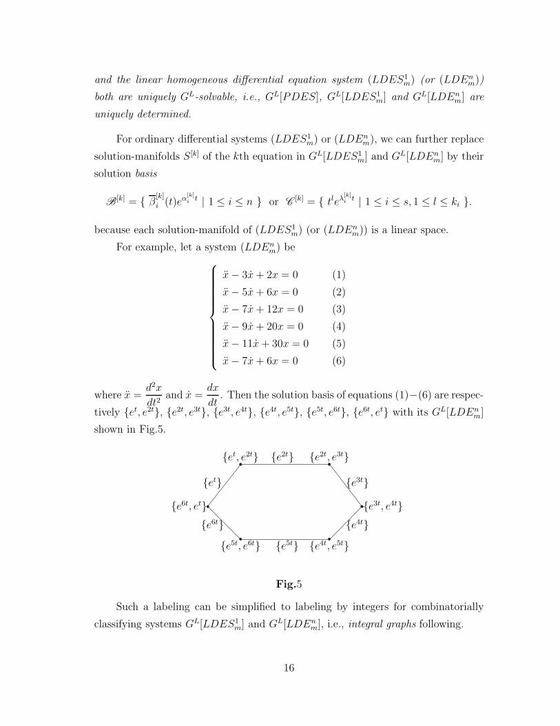
For example, let a system (LDEnm) be

x − 3x + 2x = 0 (1)

x − 5x + 6x = 0 (2)

x − 7x + 12x = 0 (3)

x − 9x + 20x = 0 (4)

x − 11x + 30x = 0 (5)

x − 7x + 6x = 0 (6)

where x =d2x

dt2and x =

dx

dt. Then the solution basis of equations (1)−(6) are respec-

tively et, e2t, e2t, e3t, e3t, e4t, e4t, e5t, e5t, e6t, e6t, et with its GL[LDEnm]

shown in Fig.5.

et, e2t e2t, e3t

e3t, e4t

e4t, e5te5t, e6t

e6t, et

e2t

e3t

e4te5t

e6t

et

Fig.5

Such a labeling can be simplified to labeling by integers for combinatorially

classifying systems GL[LDES1m] and GL[LDEn

m], i.e., integral graphs following.

16

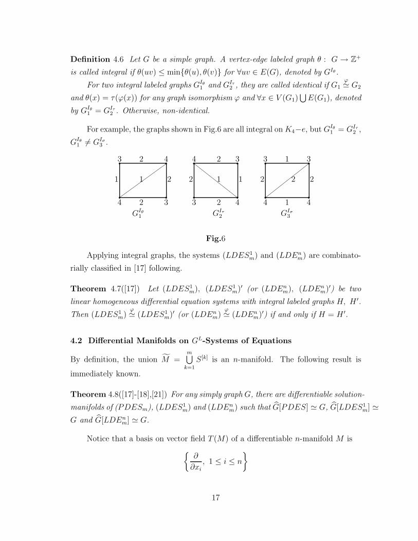
Definition 4.6 Let G be a simple graph. A vertex-edge labeled graph θ : G → Z+

is called integral if θ(uv) ≤ minθ(u), θ(v) for ∀uv ∈ E(G), denoted by GIθ .

For two integral labeled graphs GIθ

1 and GIτ

2 , they are called identical if G1

ϕ≃ G2

and θ(x) = τ(ϕ(x)) for any graph isomorphism ϕ and ∀x ∈ V (G1)⋃

E(G1), denoted

by GIθ

1 = GIτ

2 . Otherwise, non-identical.

For example, the graphs shown in Fig.6 are all integral on K4−e, but GIθ

1 = GIτ

2 ,

GIθ

1 6= GIσ

3 .

3 4

4 3

1

2

2

1 2 2 1 1

4 2

2 4

3

3

3 3

4 4

2

GIθ

1 GIτ

2

2 2

1

1

GIσ

3

Fig.6

Applying integral graphs, the systems (LDES1m) and (LDEn

m) are combinato-

rially classified in [17] following.

Theorem 4.7([17]) Let (LDES1m), (LDES1

m)′ (or (LDEnm), (LDEn

m)′) be two

linear homogeneous differential equation systems with integral labeled graphs H, H ′.

Then (LDES1m)

ϕ≃ (LDES1m)′ (or (LDEn

m)ϕ≃ (LDEn

m)′) if and only if H = H ′.

4.2 Differential Manifolds on GL-Systems of Equations

By definition, the union M =m⋃

k=1

S [k] is an n-manifold. The following result is

immediately known.

Theorem 4.8([17]-[18],[21]) For any simply graph G, there are differentiable solution-

manifolds of (PDESm), (LDES1m) and (LDEn

m) such that G[PDES] ≃ G, G[LDES1m] ≃

G and G[LDEnm] ≃ G.

Notice that a basis on vector field T (M) of a differentiable n-manifold M is

∂

∂xi

, 1 ≤ i ≤ n

17

and a vector field X can be viewed as a first order partial differential operator

X =n∑

i=1

ai

∂

∂xi

,

where ai is C∞-differentiable for all integers 1 ≤ i ≤ n. Combining Theorems 4.5

and 4.8 enables one to get a result on vector fields following.

Theorem 4.9([21]) For an integer m ≥ 1, let Ui, 1 ≤ i ≤ m be open sets in Rn

underlying a graph defined by V (G) = Ui|1 ≤ i ≤ m, E(G) = (Ui, Uj)|Ui

⋂Uj 6=

∅, 1 ≤ i, j ≤ m. If Xi is a vector field on Ui for integers 1 ≤ i ≤ m, then there

always exists a differentiable manifold M ⊂ Rn with atlas A = (Ui, φi)|1 ≤ i ≤ m

underlying graph G and a function uG ∈ Ω0(M) such that Xi(uG) = 0, 1 ≤ i ≤ m.

§5. Applications

In philosophy, every thing is a GL-system with contradictions embedded in our

world, which implies that the geometry on non-solvable system of equations is in

fact a truthful portraying of things with applications to various fields, particularly,

the understanding on gravitational fields and the controlling of industrial systems.

5.1 Gravitational Fields

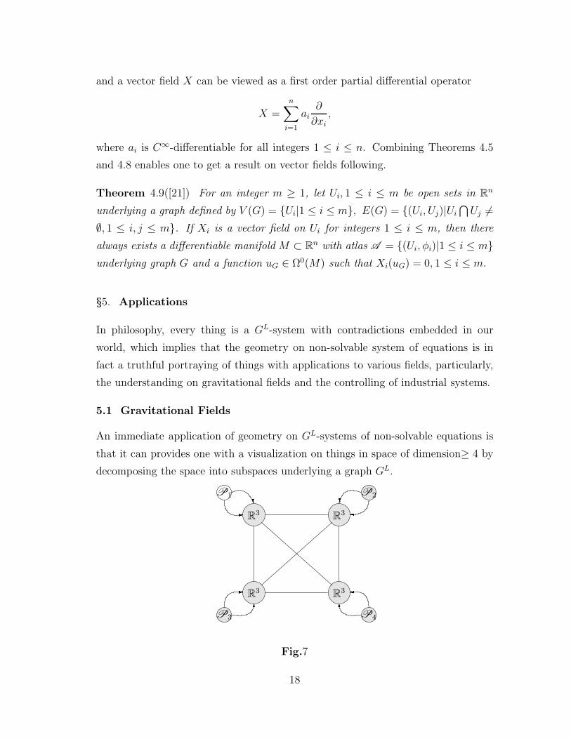
An immediate application of geometry on GL-systems of non-solvable equations is

that it can provides one with a visualization on things in space of dimension≥ 4 by

decomposing the space into subspaces underlying a graph GL.

R3 R3

R3 R3

P1 P2

P3 P4

- ? ?- 6 6

Fig.7

18

For example, a decomposition of a Euclidean space into R3 is shown in Fig.7, where

GL ≃ K4, a complete graph of order 4 and P1, P2, P3, P4 are the observations on

its subspaces R3. Notice that R3 is in a general position and R3⋂

R3 6≃ R3 here.

Generally, if GL ≃ Km, we know its dimension following.

Theorem 5.1([9],[13]) Let EKm(3) be a Km-space of R

31, · · · , R3

︸ ︷︷ ︸m

. Then its minimum

dimension

dimminEKm(3) =

3, if m = 1,

4, if 2 ≤ m ≤ 4,

5, if 5 ≤ m ≤ 10,

2 + ⌈√m⌉, if m ≥ 11

and maximum dimension

dimmaxEKm(3) = 2m − 1

with R3i

⋂R3

j =m⋂

i=1

R3i for any integers 1 ≤ i, j ≤ m.

For the gravitational field, by applying the geometrization of gravitation in R3,

Einstein got his gravitational equations with time ([1])

Rµν − 1

2Rgµν + λgµν = −8πGT µν

where Rµν = Rµανα = gαβRαµβν , R = gµνR

µν are the respective Ricci tensor, Ricci

scalar curvature, G = 6.673 × 10−8cm3/gs2, κ = 8πG/c4 = 2.08 × 10−48cm−1 ·g−1 · s2, which has a spherically symmetric solution on Riemannian metric, called

Schwarzschild spacetime

ds2 = f(t)(1 − rs

r

)dt2 − 1

1 − rs

r

dr2 − r2(dθ2 + sin2 θdφ2)

for λ = 0 in vacuum, where rg is the Schwarzschild radius. Thus, if the dimension of

the universe≥ 4, all these observations are nothing else but a projection of the true

faces on our six organs, a pseudo-truth. However, different from the string theory,

we can characterize its global behavior by KLm-space solutions of R

3 (See [8]-[10] for

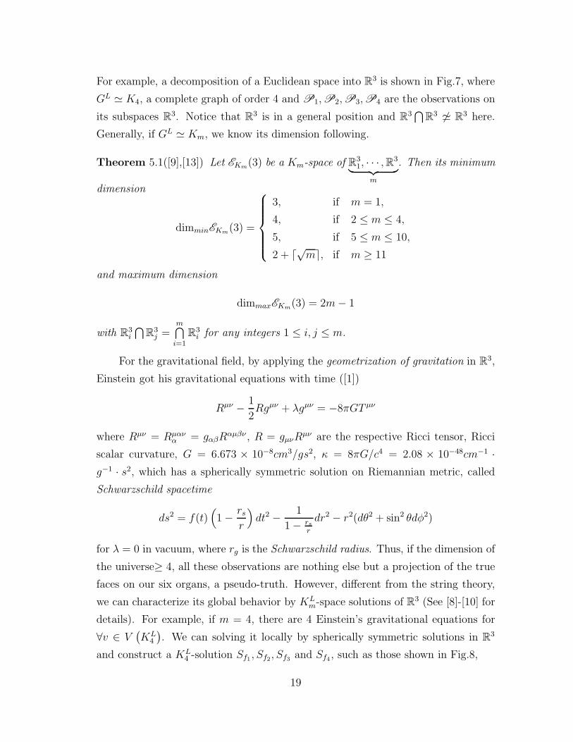
details). For example, if m = 4, there are 4 Einstein’s gravitational equations for

∀v ∈ V(KL

4

). We can solving it locally by spherically symmetric solutions in R

3

and construct a KL4 -solution Sf1 , Sf2, Sf3 and Sf4 , such as those shown in Fig.8,

19

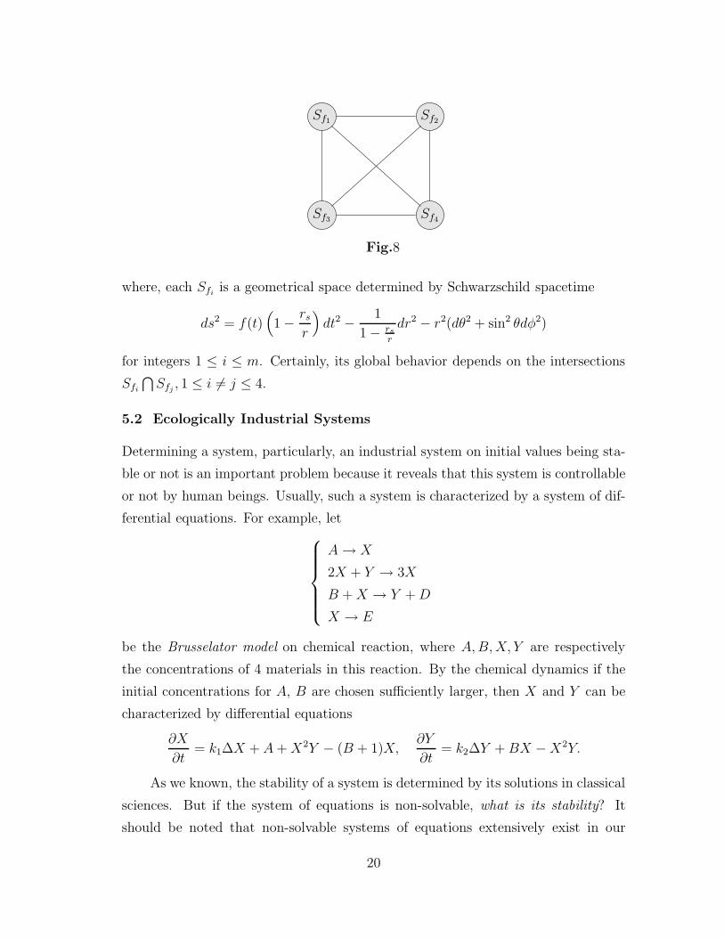
Sf1 Sf2

Sf3 Sf4

Fig.8

where, each Sfiis a geometrical space determined by Schwarzschild spacetime

ds2 = f(t)(1 − rs

r

)dt2 − 1

1 − rs

r

dr2 − r2(dθ2 + sin2 θdφ2)

for integers 1 ≤ i ≤ m. Certainly, its global behavior depends on the intersections

Sfi

⋂Sfj

, 1 ≤ i 6= j ≤ 4.

5.2 Ecologically Industrial Systems

Determining a system, particularly, an industrial system on initial values being sta-

ble or not is an important problem because it reveals that this system is controllable

or not by human beings. Usually, such a system is characterized by a system of dif-

ferential equations. For example, let

A → X

2X + Y → 3X

B + X → Y + D

X → E

be the Brusselator model on chemical reaction, where A, B, X, Y are respectively

the concentrations of 4 materials in this reaction. By the chemical dynamics if the

initial concentrations for A, B are chosen sufficiently larger, then X and Y can be

characterized by differential equations

∂X

∂t= k1∆X + A + X2Y − (B + 1)X,

∂Y

∂t= k2∆Y + BX − X2Y.

As we known, the stability of a system is determined by its solutions in classical

sciences. But if the system of equations is non-solvable, what is its stability? It

should be noted that non-solvable systems of equations extensively exist in our

20

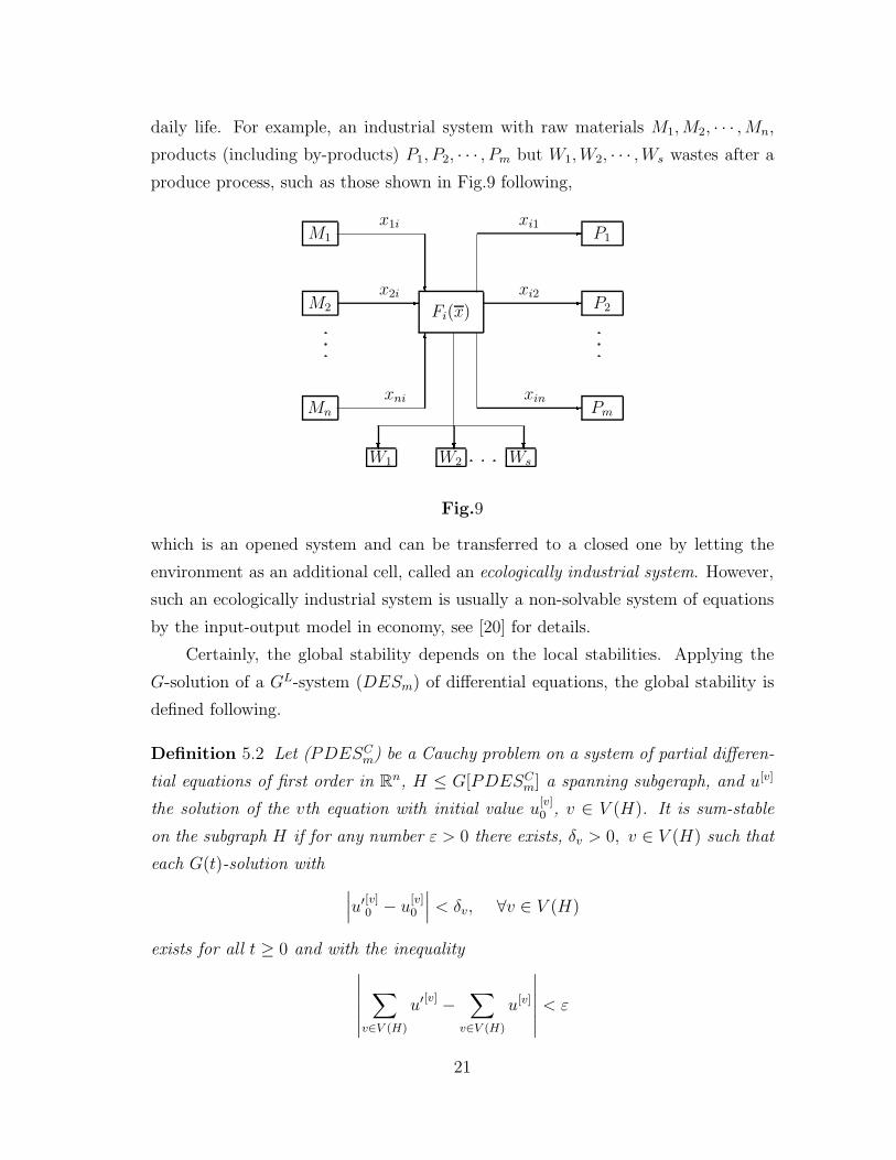
daily life. For example, an industrial system with raw materials M1, M2, · · · , Mn,

products (including by-products) P1, P2, · · · , Pm but W1, W2, · · · , Ws wastes after a

produce process, such as those shown in Fig.9 following,

Fi(x)

M1

M2

Mn

6?-x1i

x2i

xni

P1

P2

Pm

---

xi1

xi2

xin

W1 W2 Ws

? ? ?Fig.9

which is an opened system and can be transferred to a closed one by letting the

environment as an additional cell, called an ecologically industrial system. However,

such an ecologically industrial system is usually a non-solvable system of equations

by the input-output model in economy, see [20] for details.

Certainly, the global stability depends on the local stabilities. Applying the

G-solution of a GL-system (DESm) of differential equations, the global stability is

defined following.

Definition 5.2 Let (PDESCm) be a Cauchy problem on a system of partial differen-

tial equations of first order in Rn, H ≤ G[PDESC

m] a spanning subgeraph, and u[v]

the solution of the vth equation with initial value u[v]0 , v ∈ V (H). It is sum-stable

on the subgraph H if for any number ε > 0 there exists, δv > 0, v ∈ V (H) such that

each G(t)-solution with

∣∣∣u′[v]0 − u

[v]0

∣∣∣ < δv, ∀v ∈ V (H)

exists for all t ≥ 0 and with the inequality∣∣∣∣∣∣

∑

v∈V (H)

u′[v] −∑

v∈V (H)

u[v]

∣∣∣∣∣∣< ε

21

holds, denoted by G[t]H∼ G[0] and G[t]

Σ∼ G[0] if H = G[PDESCm]. Furthermore, if

there exists a number βv > 0, v ∈ V (H) such that every G′[t]-solution with

∣∣∣u′[v]0 − u

[v]0

∣∣∣ < βv, ∀v ∈ V (H)

satisfies

limt→∞

∣∣∣∣∣∣

∑

v∈V (H)

u′[v] −∑

v∈V (H)

u[v]

∣∣∣∣∣∣= 0,

then the G[t]-solution is called asymptotically stable, denoted by G[t]H→ G[0] and

G[t]Σ→ G[0] if H = G[PDESC

m].

Let (PDESCm) be a system

∂u

∂t= Hi(t, x1, · · · , xn−1, p1, · · · , pn−1)

u|t=t0 = u[i]0 (x1, x2, · · · , xn−1)

1 ≤ i ≤ m (APDESC

m)

A point X[i]0 = (t0, x

[i]10, · · · , x[i]

(n−1)0) with Hi(t0, x[i]10, · · · , x[i]

(n−1)0) = 0 for an inte-

ger 1 ≤ i ≤ m is called an equilibrium point of the ith equation in (APDESm). A

result on the sum-stability of (APDESm) is known in [18] and [21] following.

Theorem 5.3([18],[21]) Let X[i]0 be an equilibrium point of the ith equation in

(APDESm) for each integer 1 ≤ i ≤ m. If

m∑

i=1

Hi(X) > 0 andm∑

i=1

∂Hi

∂t≤ 0

for X 6=m∑

i=1

X[i]0 , then the system (APDESm) is sum-stability, i.e., G[t]

Σ∼ G[0].

Furthermore, ifm∑

i=1

∂Hi

∂t< 0

for X 6=m∑

i=1

X[i]0 , then G[t]

Σ→ G[0].

Particularly, if the non-solvable system is a linear homogenous differential equa-

tion systems (LDES1m), we further get a simple criterion on its zero GL-solution,

i.e., all vertices with 0 labels in [17] following.

22

Theorem 5.4([17]) The zero G-solution of linear homogenous differential equa-

tion systems (LDES1m) is asymptotically sum-stable on a spanning subgraph H ≤

G[LDES1m] if and only if Reαv < 0 for each βv(t)e

αvt ∈ Bv in (LDES1) hold for

∀v ∈ V (H).

References

[1] M.Carmeli, Classical Fields–General Relativity and Gauge Theory, World Sci-

entific, 2001.

[2] Fritz John. Partial Differential Equations(4th Edition). New York, USA:

Springer-Verlag, 1982.

[3] H.Iseri, Smarandache Manifolds, American Research Press, Rehoboth, NM,2002.

[4] John M.Lee, Introduction to Topological Manifolds, Springer-Verlag New York,

Inc., 2000.

[5] F.Klein, A comparative review of recent researches in geometry, Bull. New

York Math. Soc., 2(1892-1893), 215-249.

[6] Linfan Mao, Combinatorial speculation and combinatorial conjecture for math-

ematics, International J.Math. Combin. Vol.1(2007), No.1, 1-19.

[7] Linfan Mao, Geometrical theory on combinatorial manifolds, JP J.Geometry

and Topology, Vol.7, No.1(2007),65-114.

[8] Linfan Mao, Combinatorial fields-an introduction, International J. Math.Combin.,

Vol.1(2009), Vol.3, 1-22.

[9] Linfan Mao, A combinatorial decomposition of Euclidean spaces Rn with con-

tribution to visibility, International J. Math.Combin., Vol.1(2010), Vol.1, 47-64.

[10] Linfan Mao, Relativity in combinatorial gravitational fields, Progress in Physics,

Vol.3(2010), 39-50.

[11] Linfan Mao, Automorphism Groups of Maps, Surfaces and Smarandache Ge-

ometries, First edition published by American Research Press in 2005, Second

edition is as a Graduate Textbook in Mathematics, Published by The Education

Publisher Inc., USA, 2011.

[12] Linfan Mao, Smarandache Multi-Space Theory, First edition published by Hexis,

Phoenix in 2006, Second edition is as a Graduate Textbook in Mathematics,

Published by The Education Publisher Inc., USA, 2011.

23

[13] Linfan Mao, Combinatorial Geometry with Applications to Field Theory, First

edition published by InfoQuest in 2005, Second edition is as a Graduate Text-

book in Mathematics, Published by The Education Publisher Inc., USA, 2011.

[14] Linfan Mao, Graph structure of manifolds with listing, International J.Contemp.

Math. Sciences, Vol.5, 2011, No.2,71-85.

[15] Linfan Mao, A generalization of Seifert-Van Kampen theorem for fundamental

groups, Far East Journal of Math.Sciences, Vol.61 No.2 (2012), 141-160.

[16] Linfan Mao, Non-solvable spaces of linear equation systems, International J.

Math. Combin., Vol.2 (2012), 9-23.

[17] Linfan Mao, Global stability of non-solvable ordinary differential equations with

applications, International J.Math. Combin., Vol.1 (2013), 1-37.

[18] Linfan Mao, Non-solvable equation systems with graphs embedded in Rn, In-

ternational J.Math. Combin., Vol.2 (2013), 8-23, Also in Proceedings of the

First International Conference on Smarandache Multispace and Multistructure,

The Education Publisher Inc. July, 2013

[19] Linfan Mao, Geometry on GL-systems of homogenous polynomials, Interna-

tional J.Contemp. Math. Sciences, Vol.9 (2014), No.6, 287-308.

[20] Linfan Mao, A topological model for ecologically industrial systems, Interna-

tional J.Math. Combin., Vol.1 (2014), 109-117.

[21] Linfan Mao, Non-solvable partial differential equations of first order with ap-

plications, Submitted.

[22] Linfan Mao, Mathematics on non-mathematics - A combinatorial contribution,

Submitted.

[23] F.Smarandache, Paradoxist Geometry, State Archives from Valcea, Rm. Valcea,

Romania, 1969, and in Paradoxist Mathematics, Collected Papers (Vol. II),

Kishinev University Press, Kishinev, 5-28, 1997.

[24] F.Smarandache, Multi-space and multi-structure, in Neutrosophy. Neutrosophic

Logic, Set, Probability and Statistics, American Research Press, 1998.

[25] F.Smarandache, A Unifying Field in Logics. Neutrosopy: Neturosophic Proba-

bility, Set, and Logic, American research Press, Rehoboth, 1999.

[26] Wolfgang Walter, Ordinary Differential Equations, Springer-Verlag New York,

Inc., 1998.

24