Embed Size (px)
Citation preview
© 2013. Dr. M. M. Hossain & J. Ferdous Ema. This is a research/review paper, distributed under the terms of the Creative Commons Attribution-Noncommercial 3.0 Unported License http://creativecommons.org/licenses/by-nc/3.0/), permitting all non commercial use, distribution, and reproduction in any medium, provided the original work is properly cited.
Global Journal of Science Frontier Research Mathematics and Decision Sciences Volume 13 Issue 6 Version 1.0 Year 2013 Type : Double Blind Peer Reviewed International Research Journal Publisher: Global Journals Inc. (USA) Online ISSN: 2249-4626 & Print ISSN: 0975-5896
Solution of Kinematic Wave Equation Using Finite Difference Method and Finite Element Method
By Dr. M. M. Hossain & J. Ferdous Ema University of Dhaka, Bangladesh
Abstract - The Various Numerical Methods are applied to solve the spatially varied unsteady flow equations (Kinematic Wave) in predicting the discharge, depth and velocity in a river. Solutions of Kinematic Wave equations through finite difference method (Crank Nicolson) and finite element method are developed for this study. The computer program is also developed in Lahey ED Developer and for graphical representation Tecplot 7 software is used. Finally some problems are solved to understand the method.
Keywords : kinematic wave, overland flow, channel flow, finite element method, crank-nicolson method.
GJSFR-F Classification : MSC 2010: 51J15 , 81R20, 35R20
Solution of Kinematic Wave Equation Using Finite Difference Method and Finite Element Method
Strictly as per the compliance and regulations of
:
Solution of Kinematic Wave Equation Using
Finite Difference Method and Finite Element
Method Dr. M. M. Hossain
α
&
J. Ferdous
Ema
σ
Keywords : kinematic wave, overland flow, channel flow, finite element method, crank-nicolson method.
Hydrology (from Greek : Yδωρ, hudōr, "water"; and λόγoς, logos, "study")
is the
study of the movement, Distribution, and quality of water throughout the Earth and thus
addresses both the hydrologic cycle and water resources. So in the broadest sense it is the
study of water in all its phases and includes hydraulics, the physics and chemistry of
water, meteorology, geology and biology. But the word as used by the scientists and
engineers usually has a considerably narrower connotation. In this more limited sense,
“Hydrology can be defined as that branch of physical geography, which is concerned with
the origin. distributaries movement and properties of the waters of the Earth”. The study
of hydrology thus concerns itself with the occurrence and transportation of the waters
through air, Over the ground and through the strata of the earth and this includes three
important phases of what is known as the hydrological cycle, namely rainfall, runoff and
evaporation. Hydrology is therefore, bounded above by meteorology, below by geology
and at land’s end by oceanology. Engineering hydrology includes those segments of
hydrology pertinent to the design and operation of engineering projects for the control
and use of water. Hydrology means the science of water. It is a branch of earth science.
Basically it is an applied science. Domains of hydrology include hydrometeorology, surface hydrology, hydrogeology,
drainage basin management and water quality, where water plays the central role. In
general sense hydrology deals with (i)
Water resources estimation (ii) Acquisition of
processes such as precipitation, runoff and evapo-transporation.
Authors α σ
:
Department of Mathematics, University of Dhaka, Dhaka-1000, Bangladesh. E-mail : [email protected]
Notes
© 2013 Global Journals Inc. (US)
25
Globa
lJo
urna
lof
Scienc
eFr
ontie
rResea
rch
V
olum
eXIII
Issue
e
rsion
IV
VI
Yea
r
2 013
F)
)
Abstract - The Various Numerical Methods are applied to solve the spatially varied unsteady flow equations (Kinematic Wave) in predicting the discharge, depth and velocity in a river. Solutions of Kinematic Wave equations through finite difference method (Crank Nicolson) and finite element method are developed for this study. The computer program is also developed in Lahey ED Developer and for graphical representation Tecplot 7 software is used. Finally some problems are solved to understand the method.
a) Kinemtic Wave Equations From Saint Venant Equations
The St. Venant equations characterizing the dynamic flow can be written as:
Continuity: )i(qx
Q
t
A
(1)
Momentum: )A
vu(q)ss(g
x
yg
x
uu
t
u0f
0
(2)
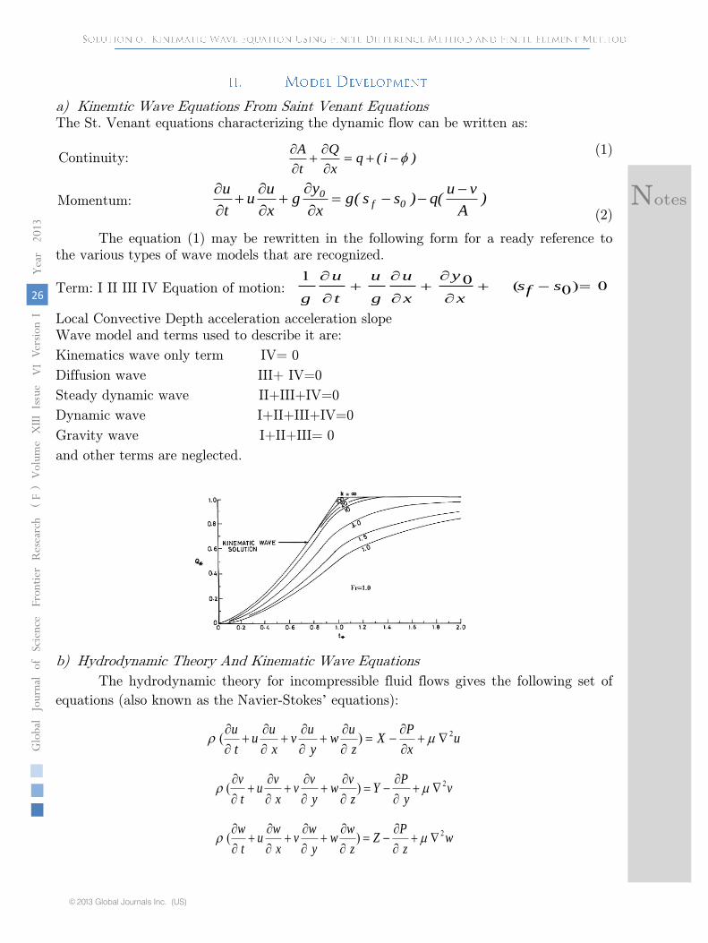
The equation (1) may be rewritten in the following form for a ready reference to
the various types of wave models that are recognized.
Term: I II III IV Equation of motion:
0)(1
00
ss
x
y
x
u
g
u
t
u
gf
Local Convective Depth acceleration acceleration slope
Wave model and terms used to describe it are:
Kinematics wave only term IV= 0
Diffusion wave III+ IV=0
Steady dynamic wave II+III+IV=0
Dynamic wave I+II+III+IV=0
Gravity wave I+II+III= 0
and other terms are neglected.
b) Hydrodynamic Theory And Kinematic Wave Equations
The hydrodynamic theory for incompressible fluid flows gives the following set of
equations (also known as the Navier-Stokes’ equations):
ux
PX
z
uw
y
uv
x
uu
t
u 2)(
vy
PY
z
vw
y
vv
x
vu
t
v 2)(
wz
PZ
z
ww
y
wv
x
wu
t
w 2)(
26
Globa
lJo
urna
lof
Scienc
eFr
ontie
rResea
rch
V
olum
eXIII
Issue
e
rsion
IV
VI
Yea
r
2013
F
)
)
© 2013 Global Journals Inc. (US)
Notes

and continuity equation: 0z
w
y
v
x
u
where ;2
2
2
2
2
22
zyx
the mass density ;
u, v and w are the velocity components in the x, y and z direction respectively;
X, Y, Z are the body forces per unit volume;
P = pressure and viscosity.
c)
Elements Used In Kinematics Wave Models
In this work, for computational purpose, the following two types of elements have
been identified:
(i)
Overland flow elements and
(ii)
Channel flow elements (Fig. 3.1)
d)
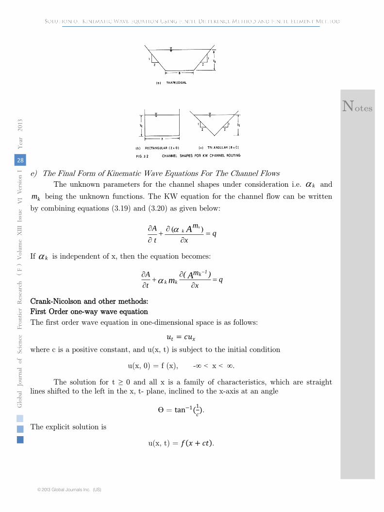
Trapezoidal Channel Cross Section
A trapezoidal cross-section is the most general type of channel cross-section. It is
defined by the cannel side slope (Z), and the channel bottom width (B) (Fig.3.2).
Notes
© 2013 Global Journals Inc. (US)
27
Globa
lJo
urna
lof
Scienc
eFr
ontie
rResea
rch
V
olum
eXIII
Issue
e
rsion
IV
VI
Yea
r
2 013
F)
)
e)
The Final Form of Kinematic Wave Equations For The Channel Flows
The unknown parameters for the channel shapes under consideration i.e. k
and
km being the unknown functions. The KW equation for the channel flow can be written
by combining equations (3.19) and (3.20) as given below:
qx
m
t
A A k
k
)(
If k
is independent of x, then the equation becomes:
qx
)m(
t
A Am
1k
kk
Crank-Nicolson and other methods:
First Order one-way wave equation
The first order wave equation in one-dimensional space is as follows:
𝑢𝑡 = 𝑐𝑢𝑥
where c is a positive constant, and u(x, t) is subject to the initial condition
u(x, 0) = f (x), -∞
<
x <
∞.
The solution for t ≥
0 and all x is a family of characteristics, which are straight
lines shifted to the left in the x, t-
plane, inclined to the x-axis at an angle
Ɵ
= tan−1(1
𝑐).
The explicit solution is
u(x, t) = 𝑓 𝑥 + 𝑐𝑡 .
28
Globa
lJo
urna
lof
Scienc
eFr
ontie
rResea
rch
V
olum
eXIII
Issue
e
rsion
IV
VI
Yea
r
2013
F
)
)
© 2013 Global Journals Inc. (US)
Notes

Finite Element Formulation for Solving KW Equation:
x
jh
jh
jxxx
h
211
)()(1
),( tj
hxM
jj
txh
Channel Discretization and Selection of Approximations Functions
The flow equations are one-dimensional. The channel is divided into small reaches
called elements. Each element will be modeled with the same flow equations but with
different channel geometry and hydraulic parameters. The elements equations are later
assembled into global matrix equations for solution. By applying the Galerkin’s principle
to the continuity equation the following equation is obtained:
Figure (A) : Finite Difference Computational Mesh
Figure (B) : Finite Element Computational Mesh
0)),((1
dxtxqx
yv
x
vy
t
yN T
x
x
K
Ii
IK
K
Notes
© 2013 Global Journals Inc. (US)
29
Globa
lJo
urna
lof
Scienc
eFr
ontie
rResea
rch
V
olum
eXIII
Issue
e
rsion
IV
VI
Yea
r
2 013
F)
)
Where 1
1
K
is the expression for summary individual element equation from 1 to
(k-1) elements; NT transpose to the shape functions.
Using the shape functions, Equations may be written as
0),(1
0
1
1
Ldstxqx
yv
x
vY
t
yN T
K
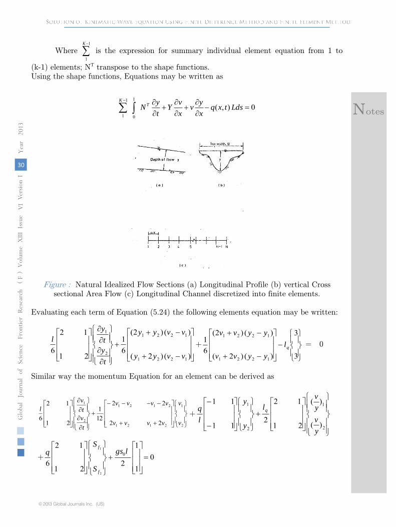
Figure
:
Natural Idealized Flow Sections (a) Longitudinal Profile (b) vertical Cross
sectional Area Flow (c) Longitudinal Channel discretized into finite elements.
Evaluating each term of Equation (5.24) the following elements equation may be written:
)()2(
)()2(
61
21
12
61221
1221
2
1
vvyy
vvyy
t
y
t
y
l+
3
3
)()2(
)()2(
61
1221
1221
ql
yyvv
yyvv
= 0
Similar way the momentum Equation for an element can be derived as
2
1
2121
2121
2
1
22
22
121
21
12
6v
v
vvvv
vvvv
t
v
t
v
l+
2
1
2
1
)(
)(
21
12
211
11
y
v
y
v
l
y
y
l
q q
+ 01
1
221
12
60
2
1
lgs
S
Sq
f
f
30
Globa
lJo
urna
lof
Scienc
eFr
ontie
rResea
rch
V
olum
eXIII
Issue
e
rsion
IV
VI
Yea
r
2013
F
)
)
© 2013 Global Journals Inc. (US)
Notes
The element properties originally expressed in local coordinates need to be
transformed into global coordinates before a solution algorithm is initated. Based on the
node to node relationship, it is possible to generate an overall element property matrix for
the entire domain, a process called assembling of element equations.
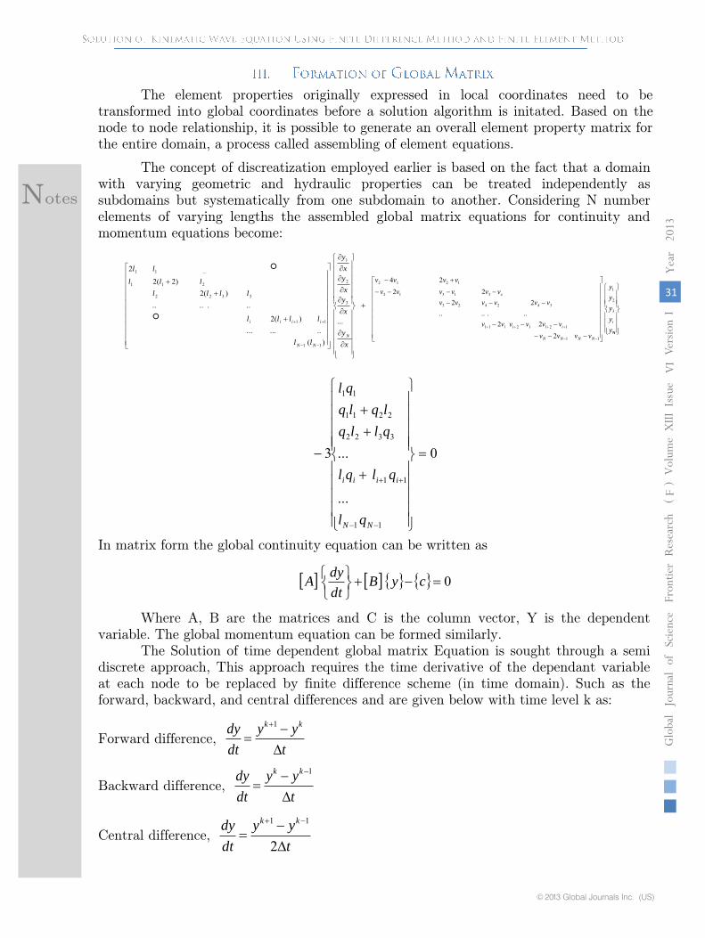
The concept of discreatization employed earlier is based on the fact that a domain
with varying geometric and hydraulic properties can be treated independently as
subdomains but systematically from one subdomain to another. Considering N number
elements of varying lengths the assembled global matrix equations for continuity and
momentum equations become:
x
y
x
y
x
y
x
y
ll
llll
llll
lll
ll
N
NN
iiii ...
)(........
)(2
.......)(2
)2(2
2
3
2
1
11
11
3322
211
...11
Ny
y
y
y
y
vvvv
vvvvvv
vvvvvv
vvvvvv
vvvv
i
NNNN
iii
z
3
2
1
11
1211211
342423
31312
1212
2
22.......
2222
24
0
...
...3
11
11
3322
2211
11
NN
iiii
ql
qlql
qllq
lqlq
ql
In matrix form the global continuity equation can be written as
0
cyBdt
dyA
Where A, B are the matrices and C is the column vector, Y is the dependent
variable. The global momentum equation can be formed similarly.
The Solution of time dependent global matrix Equation is sought through a semi
discrete approach, This approach requires the time derivative of the dependant variable
at each node to be replaced by finite difference scheme (in time domain). Such as the
forward, backward, and central differences and are given below with time level k as:
Forward difference, t
yy
dt
dy kk
1
Backward difference, t
yy
dt
dy kk
1
Central difference, t
yy
dt
dy kk
2
11
Notes
© 2013 Global Journals Inc. (US)
31
Globa
lJo
urna
lof
Scienc
eFr
ontie
rResea
rch
V
olum
eXIII
Issue
e
rsion
IV
VI
Yea
r
2 013
F)
)

An implicit equation will be generated from this Equation with the aid of the time
weighting factor in the next section.
Development of the Numerical models
The deterministic stream flow models are investigated with three distinct options:
(1) the kinematic flow models comprises (a) the simplified version of momentum equation
that neglects pressure and inertia terms are compared to friction and gravity terms and
(b) the complete form of continuity equation; (2) the diffusion flow models comprises (a)
the simplified momentum equation that accounts only for pressure, friction, and gravity
terms and (b) the complete form of continuity equation; and (3) the complete flow model
comprises (a) the complete form of momentum equation and (b) the complete continuity
equation.
The kinematic flow model is investigated in both explicit and implicit sense. The
explicit kinematic flow model leads to linear equations. They are solved using a direct
method similar to the tridiagonal matrix algorithm set up by varga (1962). The solution
proceeds by matrix reduction similar to Gaussian elimination. In contrast the explicit
model, the implicit kinematic model yields a set of non-linear tridiagonal matrix equations
which are solved by the functional Newton-Raphson iterative method.
The diffusion model as well as the complete flow model each results in a non-linear
bitridiagonal matrix equation. The functional Newton-Raphson’s method, along with the
direct solution algorithm, triangular decomposition technique that yields a recursion
algorithm (Douglas, et al, 1959, Von Rosenberg, 1969), is utilized to predict depth and
velocity of flow for each option.
Finite Element Kinematic Wave Model
Explicit Model:
The non-linear continuity equation is easily converted to linear form by use of
geometric and flow relations:
𝜕𝐴
𝜕𝑡+
𝜕𝑄
𝜕𝑥−
𝑞 𝑥, 𝑡 = 0
Where, A = Area of flow,
𝐿2
;
Q = volumetric flow rate, 𝐿3
𝑇
The appropriate simplified momentum equation for coupling with the continuity
equation has been obtained and is presented below
𝑆𝑓 =
𝑆0 =
𝑛1
2 𝑣2
𝑅4
3 =
𝑣2𝑅4
3
𝑀2
Or 𝑄 =
𝐴𝑅2
3 𝑆0
12
𝑛1
=
𝑀𝐴𝑅2
3
𝑆0
12
These equations are written in matrix units. For fps units first equation to be
divided by 2.216 and the second equation to be multiplied by 1.486.
32
Globa
lJo
urna
lof
Scienc
eFr
ontie
rResea
rch
V
olum
eXIII
Issue
e
rsion
IV
VI
Yea
r
2013
F
)
)
© 2013 Global Journals Inc. (US)
Substitution of Equation (5.29a) in Equation (5.28) yields
01
cyBt
yyA k
kk
Notes
2
1
2 11
11
21
21
12
6Q
Q
t
A
t
A
lj
- 01
1
2
ql
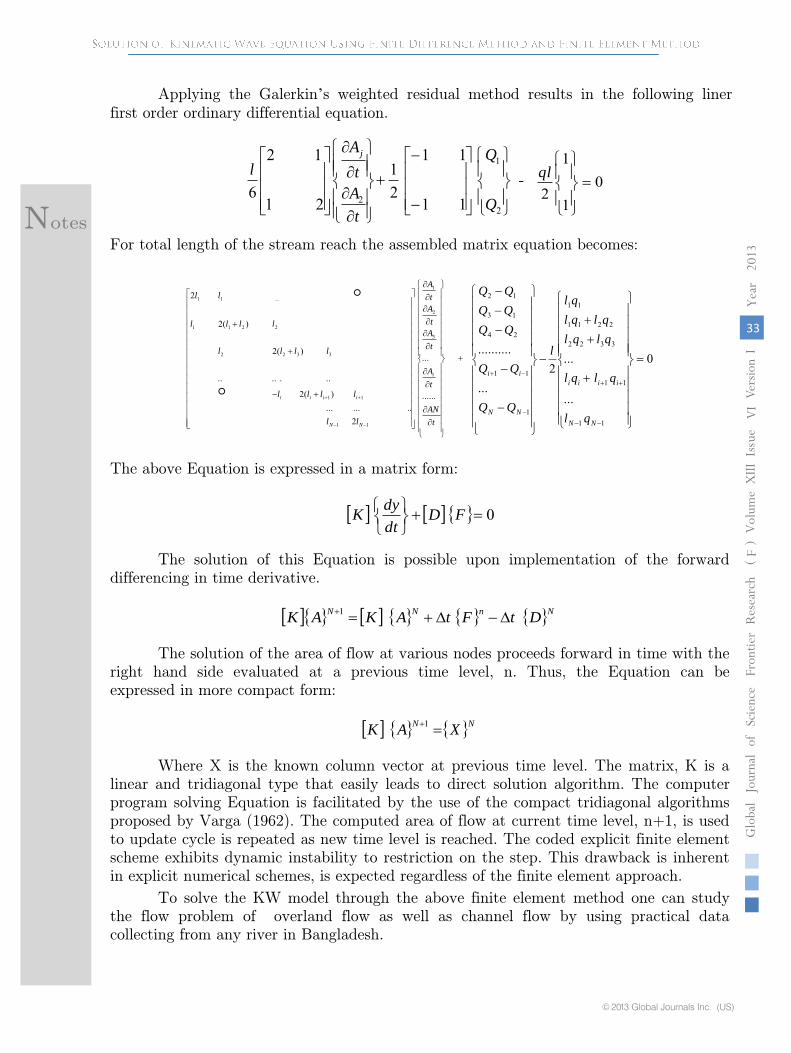
For total length of the stream reach the assembled matrix equation becomes:
t
AN
t
A
t
A
t
A
t
A
ll
llll
llll
llll
ll
i
NN
iiii ......
...
2........
)(2
.......
)(2
)(2
2
3
2
1
11
11
3322
2211
...11
0
...
...2
...
..........
11
11
3322
2211
11
1
11
24
13
12
NN
iiii
NN
ii
ql
qlql
qlql
qlql
ql
l
The above Equation is expressed in a matrix form:
0
FDdt
dyK
The solution of this Equation is possible upon implementation of the forward
differencing in time derivative.
NnNNDtFtAKAK
1
The solution of the area of flow at various nodes proceeds forward in time with the
right hand side evaluated at a previous time level, n. Thus, the Equation can be
expressed in more compact form:
NNXAK
1
Where X is the known column vector at previous time level. The matrix, K is a
linear and tridiagonal type that easily leads to direct solution algorithm. The computer
program solving Equation is facilitated by the use of the compact tridiagonal algorithms
proposed by Varga (1962). The computed area of flow at current time level, n+1, is used
to update cycle is repeated as new time level is reached. The coded
explicit finite element
scheme exhibits dynamic instability to restriction on the step. This drawback is inherent
in explicit numerical schemes, is expected regardless of the finite element approach.
To solve the KW model through the above finite element
method one can study
the flow problem of overland flow as well as channel flow by using practical data
collecting from any river in Bangladesh.
Notes
© 2013 Global Journals Inc. (US)
33
Globa
lJo
urna
lof
Scienc
eFr
ontie
rResea
rch
V
olum
eXIII
Issue
e
rsion
IV
VI
Yea
r
2 013
F)
)
Applying the Galerkin’s weighted residual method results in the following liner
first order ordinary differential equation.
that the dynamic approached are the best to account for the physical processes associated
with the runoff mechanics of the watersheds. Among these approaches, the kinematic
wave theory is the best suited to the prevailing condition.
A further work can be done by developing computer program using these methods
to solve KW equation for channel
and overland flows for various practical data set
collecting from any small river in Bangladesh
1.
Amien,
M.,
and
Chu, H.L.
(1975).
Implicit Numerical Modeling of
Unsteady Flows.
J. of Hydr. Div., Proc. ASCE., Vol. 101(HY1):
717-731.
2.
Amien, M., and
Fang, C.S.
(1970).Implicit Flood routing in Natural Channels.
J. of Hyd. Div., Proc. ASCE, Vol.96 (HY12):
2481-2500.
3.
Brakensick, D.L.
(1967A).
A Simulated Watershed Flow System for Hydrograph
Prediction: A Kinematics Application. Paper No.3,
Proc. Of the Intl. Hydrology Symp, Fort Colino, Colardo.
4.
Cambell, S.Y., Parlange, J.Y. and
Rose, C.W.
(1984).
Overland Flow on Converging
and Diverging Surfaces-Kinematics model and Similarly Solutions.
J. Hydrology, Vol. (67): 367-374.
5.
Carnahan, B., Luther, H.A., and
Wilkes, J.O.
(1969).
Applied Numerical Methods. John Willy, New York.
6.
Cow, V.T.
(1959).
Open channel Hydraulics.
McGraw-Hill Book Company. New York.
7.
Clark, C.O.
(1945). Storage and the Unit Hydrograph.
Proc. ASCE, Vol. 69: 1333-
1360.
8.
Clarke, R.T
(1973).
Mathematical Models in Hydrology.
Food and Agri. Organ. Of the United Nations, Irrigation and Drainage paper No. 19, Rome.
9.
Cooley, R.L., and
Moin, S.A.
(1976).
Finite Element Solution of St. Venant
Equations.
J. of Hyd. Div., Proc. ASCE, Vol. 102(NY6): 759-775.
10.
Dooge, J.C.I.
(1959).
A General Theory of the Unit Hydrograph.
Journal of Geophysical Res., AUG, 64(2):241-256
11.
DeVriesm J.J., and
MacArthur, R. C.
(1979).
Introduction and Application of
Kinematics Wave Routing Techniques Using HEC-1. Training Doc. No. 10,
HEC, DAVIS, California, USA.
12.
Dooge, J.C.I.
(1969).
A General Theory of the Unit Hydrograph.
Journal of Geophysical Res., AUG, 64(2): 241-256.
13.
Dooge, J.C.I.
(1973).
Linear Theory of Hydrologic Systems.
U.S. Dept. Agri., Agri. Res. Serv., Tech. Bull. 1468, 327 pp.
14.
Freeze, R.A.
(1978).
Mathematical Models of Hill slope Hydrology, in Hill slope
Hydrology, M.J. Kirkby, eds.,
John Wiley & Sons Ltd., New York.
15.
Hossain, M. M.
(1989).
Application of Kinematics Wave Theory to Small Watersheds
Ph.D. Thesis. Submitted in the
Roorkee University, UP, India.
34
Globa
lJo
urna
lof
Scienc
eFr
ontie
rResea
rch
V
olum
eXIII
Issue
e
rsion
IV
VI
Yea
r
2013
F
)
)
© 2013 Global Journals Inc. (US)
suitable surface hydrological model for study the movement of overland, (i.e. through its
surface runoff) as well as stream flow components of the hydrologic cycle. To achieve
these objectives, various techniques and available models were studied. It was concluded
A hydrological model is an important tool for estimating and organizing
quantitative hydrologic information. The main objectives of this thesis is to develop a
Notes
20.
Nash, J.E.
(1957).
The Form of Instantaneous Unit Hydrograph.
IASH General Assembly, Toronto, Pub.45:
114-119.
21.
Nash, J.E.
(1960).
A unit Hydrograph Study with Particular Reference to British
Catchments.
Proc. Inst, Civ. Engrs., No. 17,
PP:
249-281.
22.
Noye, J.
(1982).
Numerical Solutions of Partial Differential Equations.
North-Holland Publishing Company, Amsterdam.
23.
Overton, D.E. and Meadows, M.E.
(1976).
Storm water Modeling.
Academic Press, New York.
24.
Parlangem J.Y., Rose, C.W. and
Sander, G.C.
(1981).
Kinematics Flow
Approximation of runoff on a plane: An exact analytical solution.
J.
Hydrol. Vol. 52:
171-178.
25.
Pederson, J. T., Peters, J.C. and
Helweg, O.J.
(1980).
Hydrographs by Single Linear
Reservoir Model.
J. of Hydr. Div. ASEC, Vol.106 (HY5):
837-652.
26.
Randkivi, A.J
(1979). Hydrology.
Pergaman Press, England
27.
Rose, C. W., Parlange. J.Y., Sander, G.C.,
Cambell, S.Y. and Barry.
D.A.
(1983).
Kinematics Flow Approximation to Runoff on a Plane: An Approximate Analytic
Solution.
J. Hydrol., Vol62:
363-369.
Notes
© 2013 Global Journals Inc. (US)
35
Globa
lJo
urna
lof
Scienc
eFr
ontie
rResea
rch
V
olum
eXIII
Issue
e
rsion
IV
VI
Yea
r
2 013
F)
)
16. King, I.P. (1977). Finite Element Methods for Unsteady Flow Through Irregular
Channels. Proc. First Conf. on Finite Elements in Water Resoures, Princeton Univ., U.S.A., July 1976; Finite Elements in Water Resources, Pentech Press, PP: 165-184.
17. Mathur, B. S. (2972). Runoff Hydrographs for Uneven Spatial Distribution of Rainfall
Ph.D. thesis, The Indian Institute of Tech., New Delhi, India.
18. Moore. I.D. et al. (1985). Kinematics Overland Flow: Generalization of Rose’s approximate Solution. J. of Hydrology, Vol. 82: 233-245
19. Moore. I.D. et al. (1985). Kinematics Overland Flow: Generalization of Rose’s approximate Solution. Part II, J, of Hydrol., Vol. 92: 351-362