Acoustic Wave Equation

Sjoerd de Ridder (most of the slides) & Biondo Biondi

January 16th 2011

Table of Topics

I Basic Acoustic Equations

I Wave Equation

I Finite Differences

I Finite Difference Solution

I Pseudospectral Solution

I Stability and Accuracy

I Green’s function

I Perturbation Representation

I Born Approximation

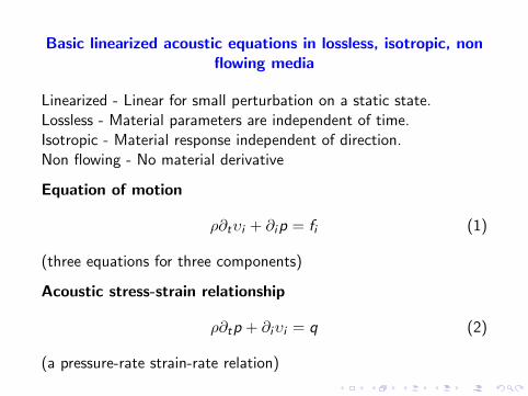
Basic linearized acoustic equations in lossless, isotropic, nonflowing media

Linearized - Linear for small perturbation on a static state.Lossless - Material parameters are independent of time.Isotropic - Material response independent of direction.Non flowing - No material derivative

Equation of motion

ρ∂tυi + ∂ip = fi (1)

(three equations for three components)

Acoustic stress-strain relationship

ρ∂tp + ∂iυi = q (2)

(a pressure-rate strain-rate relation)

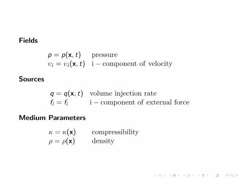
Fields

p = p(x, t) pressureυi = υi (x, t) i− component of velocity

Sources

q = q(x, t) volume injection ratefi = fi i− component of external force

Medium Parameters

κ = κ(x) compressibilityρ = ρ(x) density

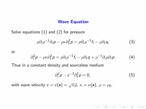
Wave Equation

Solve equations (1) and (2) for pressure

ρ∂iρ−1∂ip − ρκ∂2

t p = ρ∂iρ−1fi − ρ∂tq, (3)

or∂2

i p − ρκ∂2t p = ρ∂iρ

−1fi − ρ∂tq + ρ−1∂iρ∂ip. (4)

Thus in a constant density and sourceless medium

∂2i p − c−2∂2

t p = 0, (5)

with wave velocity c = c(x) =√

κρ, κ = κ(x), ρ = ρ0.

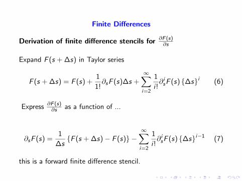
Finite Differences

Derivation of finite difference stencils for ∂F (s)∂s

Expand F (s + ∆s) in Taylor series

F (s + ∆s) = F (s) +1

1!∂sF (s)∆s +

∞∑i=2

1

i !∂ i

sF (s) {∆s}i (6)

Express ∂F (s)∂s as a function of ...

∂sF (s) =1

∆s{F (s + ∆s)− F (s)} −

∞∑i=2

1

i !∂ i

sF (s) {∆s}i−1 (7)

this is a forward finite difference stencil.

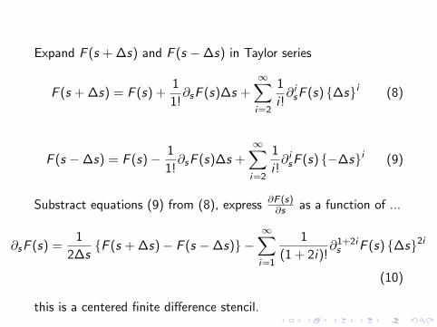
Expand F (s + ∆s) and F (s −∆s) in Taylor series

F (s + ∆s) = F (s) +1

1!∂sF (s)∆s +

∞∑i=2

1

i !∂ i

sF (s) {∆s}i (8)

F (s −∆s) = F (s)− 1

1!∂sF (s)∆s +

∞∑i=2

1

i !∂ i

sF (s) {−∆s}i (9)

Substract equations (9) from (8), express ∂F (s)∂s as a function of ...

∂sF (s) =1

2∆s{F (s + ∆s)− F (s −∆s)} −

∞∑i=1

1

(1 + 2i)!∂1+2i

s F (s) {∆s}2i

(10)

this is a centered finite difference stencil.

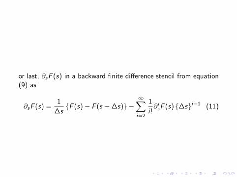
or last, ∂sF (s) in a backward finite difference stencil from equation(9) as

∂sF (s) =1

∆s{F (s)− F (s −∆s)} −

∞∑i=2

1

i !∂ i

sF (s) {∆s}i−1 (11)

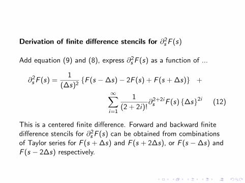
Derivation of finite difference stencils for ∂2s F (s)

Add equation (9) and (8), express ∂2s F (s) as a function of ...

∂2s F (s) =

1

(∆s)2{F (s −∆s)− 2F (s) + F (s + ∆s)} +

∞∑i=1

1

(2 + 2i)!∂2+2i

s F (s) {∆s}2i (12)

This is a centered finite difference. Forward and backward finitedifference stencils for ∂2

s F (s) can be obtained from combinationsof Taylor series for F (s + ∆s) and F (s + 2∆s), or F (s −∆s) andF (s − 2∆s) respectively.

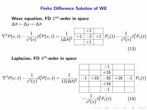
Finite Difference Solution of WE

Wave equation, FD 2nd -order in space∆h = ∆y = ∆h

∇2P(x , t)− 1

c2(x)∂2

t P(x , t) =1

(∆h)2

+1

+1 −2 +1

+1

Px(t)−1

c2(x)∂2

t Px(t)

(13)

Laplacian, FD 4th-order in space

∇2P(x , t)− 1

c2(x)∂2

t P(x , t) =1

12(∆h)2

−1

+16

−1 +16 −30 +16 −1

+16

−1

Px(t)

− 1

c2(x)∂2

t Px(t) (14)

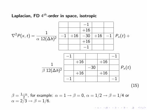
Laplacian, FD 4th-order in space, isotropic

∇2P(x , t) =1

α 12(∆h)2

−1

+16

−1 +16 −30 +16 −1

+16

−1

Px(t) +

1

β 12(∆h)2

−1 −1

+16 +16

−30

+16 +16

−1 −1

Px(t)

(15)

β = 1−α2 , for example: α = 1 → β = 0, α = 1/2 → β = 1/4 or

α = 2/3 → β = 1/6.

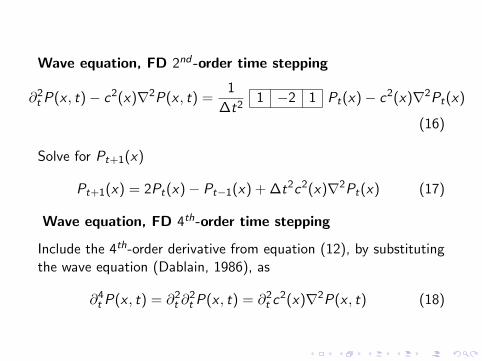
Wave equation, FD 2nd -order time stepping

∂2t P(x , t)− c2(x)∇2P(x , t) =

1

∆t21 −2 1 Pt(x)− c2(x)∇2Pt(x)

(16)

Solve for Pt+1(x)

Pt+1(x) = 2Pt(x)− Pt−1(x) + ∆t2c2(x)∇2Pt(x) (17)

Wave equation, FD 4th-order time stepping

Include the 4th-order derivative from equation (12), by substitutingthe wave equation (Dablain, 1986), as

∂4t P(x , t) = ∂2

t ∂2t P(x , t) = ∂2

t c2(x)∇2P(x , t) (18)

Pseudospectral (Fourier) methods

I Laplacian computed using FFTs:

c2 (x)∇2Pt (x) ≈ c2 (x) FFT−1

{−

∣∣∣~k∣∣∣2 FFT [Pt (x)]

}

I Wave equation, FD 2nd-order time stepping andpseudospectral Laplacian:Pt+1 (x) =

2Pt (x)− Pt−1 (x) + ∆t2c2 (x) FFT−1

{−

∣∣∣~k∣∣∣2 FFT [Pt (x)]

}

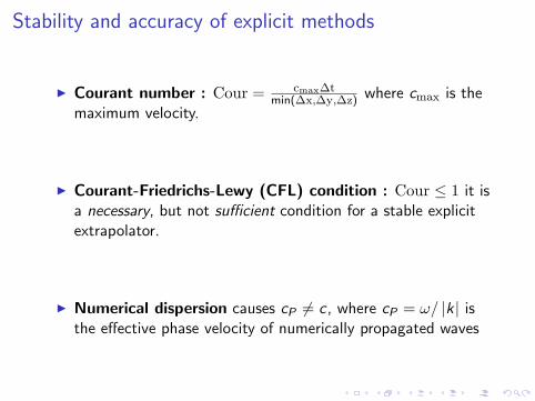
Stability and accuracy of explicit methods

I Courant number : Cour = cmax∆tmin(∆x,∆y,∆z) where cmax is the

maximum velocity.

I Courant-Friedrichs-Lewy (CFL) condition : Cour ≤ 1 it isa necessary, but not sufficient condition for a stable explicitextrapolator.

I Numerical dispersion causes cP 6= c , where cP = ω/ |k| isthe effective phase velocity of numerically propagated waves

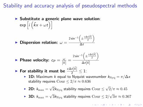
Stability and accuracy analysis of pseudospectral methods

I Substitute a generic plane wave solution:

exp[i(~kx + ωt

)]

I Dispersion relation: ω =2 sin−1

„± c∆t|~k|

2

«∆t

I Phase velocity: cP = ω

|~k| =2 sin−1

„± c∆t|~k|

2

«∆t|~k|

I For stability it must bec∆t|~k|

2 ≤ 1:I 1D: Maximum k equal to Nyquist wavenumber kNyq = π/∆x

stability requires Cour ≤ 2/π ≈ 0.636

I 2D: kmax =√

2kNyq stability requires Cour ≤√

2/π ≈ 0.45

I 3D: kmax =√

3kNyq stability requires Cour ≤ 2/√

3π ≈ 0.367

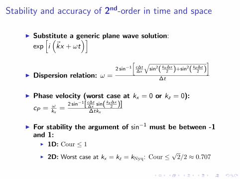
Stability and accuracy of 2nd-order in time and space

I Substitute a generic plane wave solution:

exp[i(~kx + ωt

)]

I Dispersion relation: ω =2 sin−1

»c∆t∆x

qsin2( kx∆x

2 )+sin2( kz∆z2 )

–∆t

I Phase velocity (worst case at kx = 0 or kz = 0):

cP = ωkx

=2 sin−1[ c∆t

∆xsin( kx∆x

2 )]∆tkx

I For stability the argument of sin−1 must be between -1and 1:

I 1D: Cour ≤ 1

I 2D: Worst case at kx = kz = kNyq: Cour ≤√

2/2 ≈ 0.707

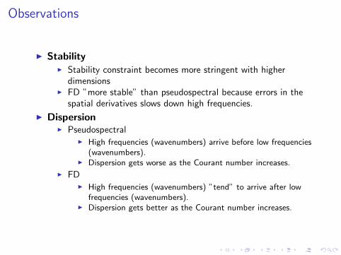
Observations

I StabilityI Stability constraint becomes more stringent with higher

dimensionsI FD ”more stable” than pseudospectral because errors in the

spatial derivatives slows down high frequencies.

I DispersionI Pseudospectral

I High frequencies (wavenumbers) arrive before low frequencies(wavenumbers).

I Dispersion gets worse as the Courant number increases.

I FDI High frequencies (wavenumbers) ”tend” to arrive after low

frequencies (wavenumbers).I Dispersion gets better as the Courant number increases.

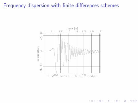
Frequency dispersion with finite-differences schemes

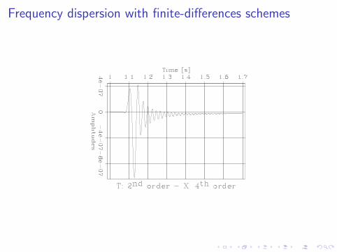
Frequency dispersion with finite-differences schemes

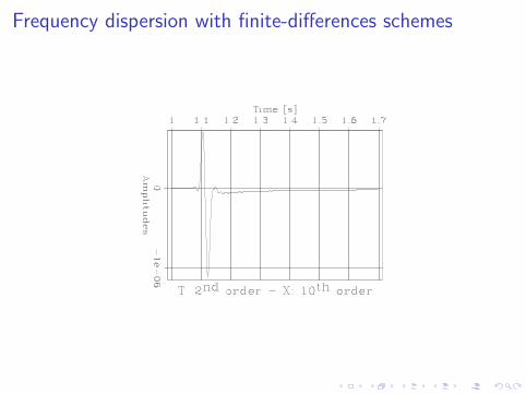
Frequency dispersion with finite-differences schemes

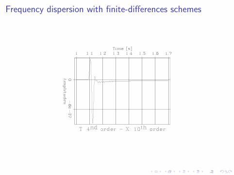
Frequency dispersion with finite-differences schemes

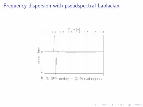
Frequency dispersion with pseudspectral Laplacian

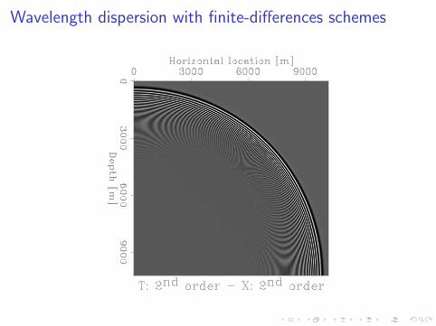
Wavelength dispersion with finite-differences schemes

Wavelength dispersion with finite-differences schemes

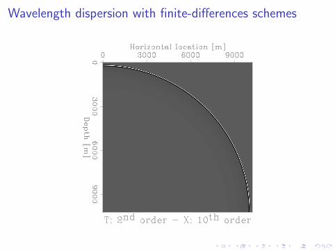
Wavelength dispersion with finite-differences schemes

Wavelength dispersion with finite-differences schemes

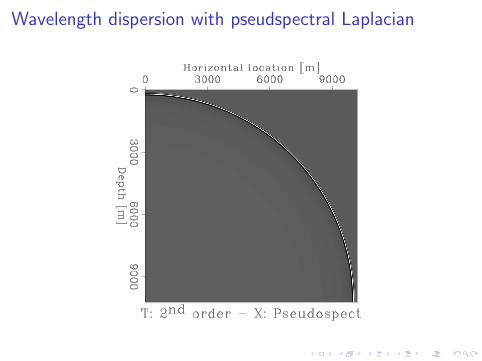
Wavelength dispersion with pseudspectral Laplacian

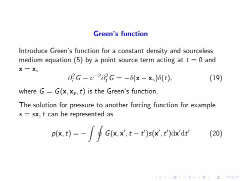
Green’s function

Introduce Green’s function for a constant density and sourcelessmedium equation (5) by a point source term acting at t = 0 andx = xs

∂2i G − c−2∂2

t G = −δ(x− xs)δ(t), (19)

where G = G (x, xs , t) is the Green’s function.

The solution for pressure to another forcing function for examples = sx, t can be represented as

p(x, t) = −∫ ∮

G (x, x′, t − t ′)s(x′, t ′)dx′dt ′ (20)

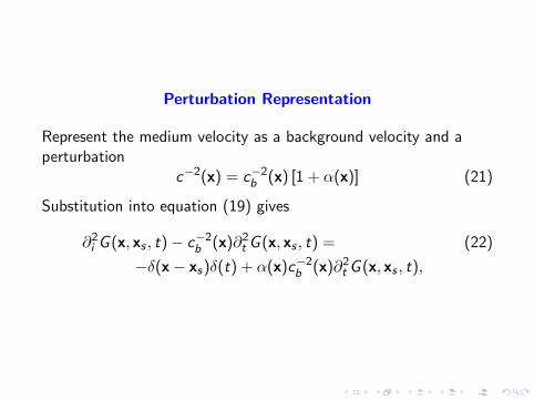
Perturbation Representation

Represent the medium velocity as a background velocity and aperturbation

c−2(x) = c−2b (x) [1 + α(x)] (21)

Substitution into equation (19) gives

∂2i G (x, xs , t)− c−2

b (x)∂2t G (x, xs , t) = (22)

−δ(x− xs)δ(t) + α(x)c−2b (x)∂2

t G (x, xs , t),

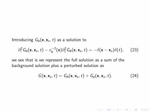
Introducing Gb(x, xs , t) as a solution to

∂2i Gb(x, xs , t)− c−2

b (x)∂2t Gb(x, xs , t) = −δ(x− xs)δ(t), (23)

we see that is we represent the full solution as a sum of thebackground solution plus a perturbed solution as

G (x, xs , t) = Gb(x, xs , t) + Gp(x, xs , t). (24)

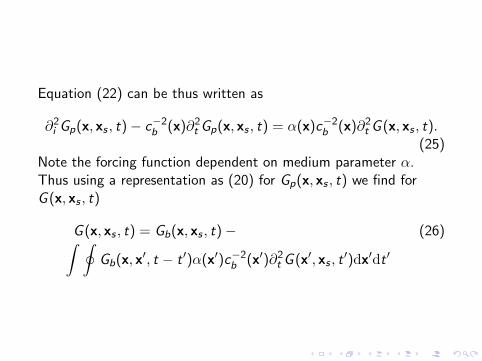
Equation (22) can be thus written as

∂2i Gp(x, xs , t)− c−2

b (x)∂2t Gp(x, xs , t) = α(x)c−2

b (x)∂2t G (x, xs , t).

(25)Note the forcing function dependent on medium parameter α.Thus using a representation as (20) for Gp(x, xs , t) we find forG (x, xs , t)

G (x, xs , t) = Gb(x, xs , t)− (26)∫ ∮Gb(x, x

′, t − t ′)α(x′)c−2b (x′)∂2

t G (x′, xs , t′)dx′dt ′

Born Approximation

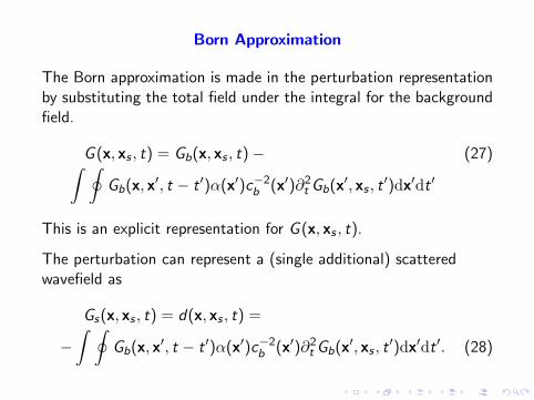
The Born approximation is made in the perturbation representationby substituting the total field under the integral for the backgroundfield.

G (x, xs , t) = Gb(x, xs , t)− (27)∫ ∮Gb(x, x

′, t − t ′)α(x′)c−2b (x′)∂2

t Gb(x′, xs , t

′)dx′dt ′

This is an explicit representation for G (x, xs , t).

The perturbation can represent a (single additional) scatteredwavefield as

Gs(x, xs , t) = d(x, xs , t) =

−∫ ∮

Gb(x, x′, t − t ′)α(x′)c−2

b (x′)∂2t Gb(x

′, xs , t′)dx′dt ′. (28)