Solar MPPT Solar MPPT TechniquesTechniques

Geno GargasGeno Gargas

ECE 548ECE 548Prof. KhalighProf. Khaligh

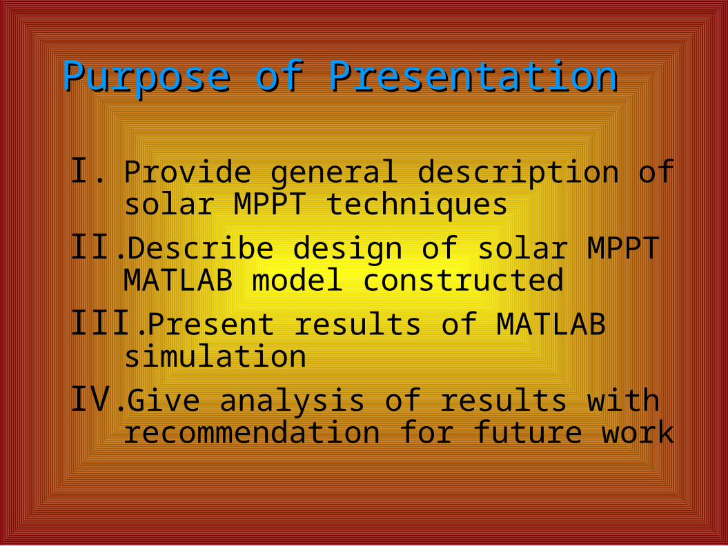
Purpose of PresentationPurpose of Presentation

I. Provide general description of solar MPPT techniques

II. Describe design of solar MPPT MATLAB model constructed

III. Present results of MATLAB simulation

IV. Give analysis of results with recommendation for future work

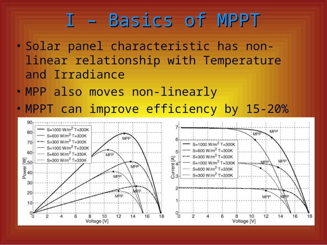
I – Basics of MPPTI – Basics of MPPT• Solar panel characteristic has non-linear relationship

with Temperature and Irradiance

• MPP also moves non-linearly

• MPPT can improve efficiency by 15-20%

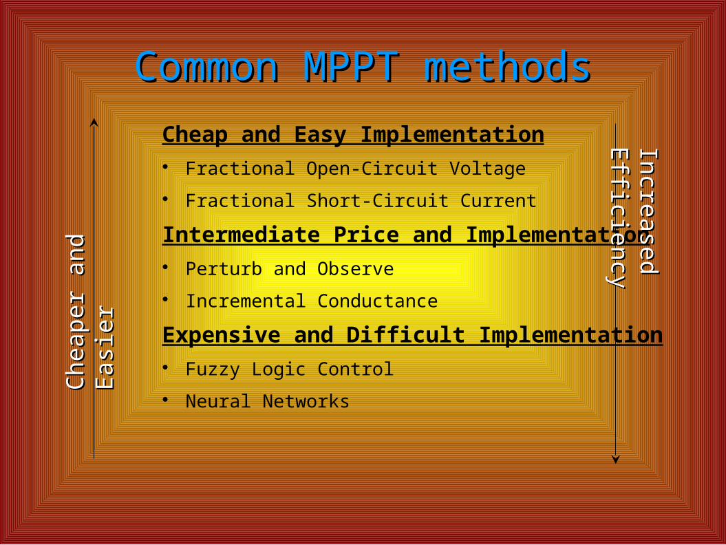
Common MPPT methodsCommon MPPT methods

Cheap and Easy Implementation Fractional Open-Circuit Voltage

Fractional Short-Circuit Current

Intermediate Price and Implementation Perturb and Observe

Incremental Conductance

Expensive and Difficult Implementation Fuzzy Logic Control

Neural Networks

Incre

ase

d E

fficie

ncy

Incre

ase

d E

fficie

ncy

Ch

eap

er

an

d E

asi

er

Ch

eap

er

an

d E

asi

er

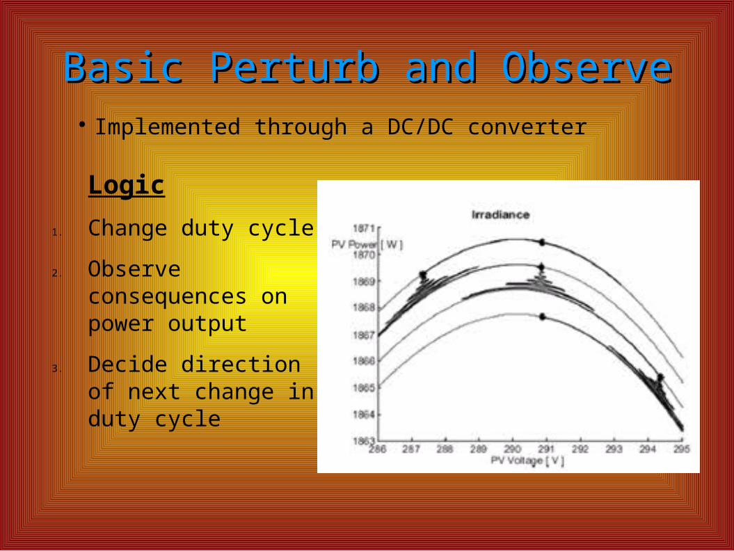
Basic Perturb and ObserveBasic Perturb and Observe Implemented through a DC/DC converter

Logic

1. Change duty cycle

2. Observe consequences on power output

3. Decide direction of next change in duty cycle

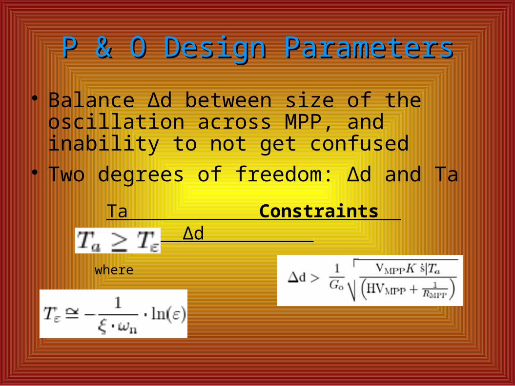
P & O Design ParametersP & O Design Parameters

Balance Δd between size of the oscillation across MPP, and inability to not get confused

Two degrees of freedom: Δd and Ta

Ta Constraints Δd

where

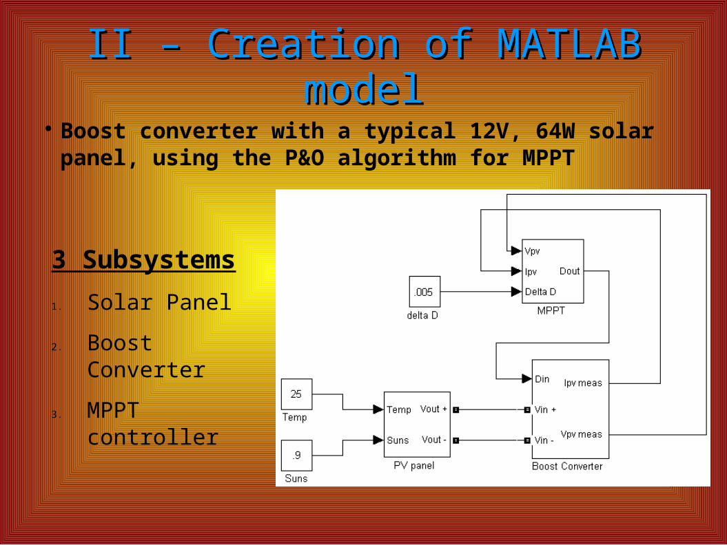
II – Creation of MATLAB modelII – Creation of MATLAB model Boost converter with a typical 12V, 64W solar

panel, using the P&O algorithm for MPPT

3 Subsystems

1. Solar Panel

2. Boost Converter

3. MPPT controller

1 - PV model design1 - PV model design

Vout -

2

Vout +

1

ih

Vpv

v+-

Rs

Rh

Photocurrent 1

s

-+

Photocurrent

s -+

Ipv control

Vpv

Ipv

Ih

Temp

Ipv s

Ipv

i+ -

Ih control

Temp

Suns

Ih s

Ih

i+ -

Diode

Suns

2

Temp

1

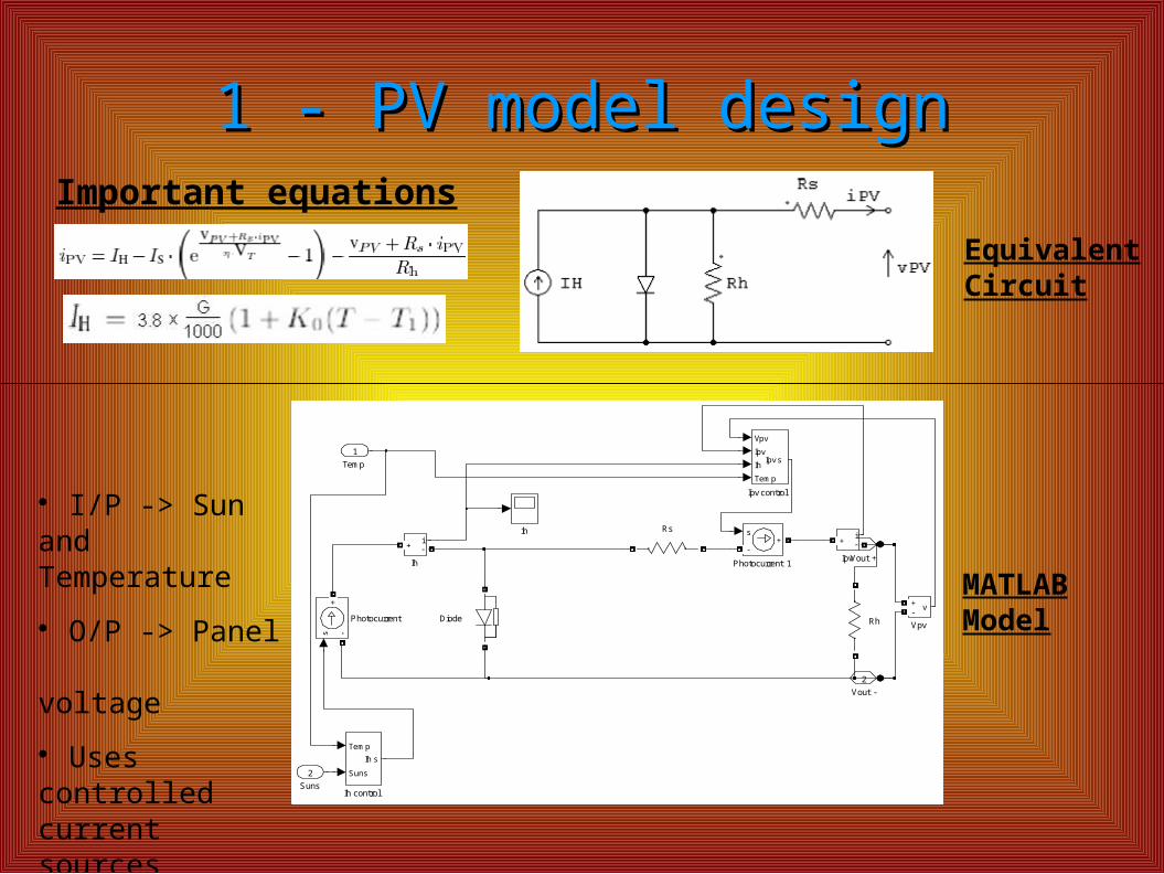
Important equations

Equivalent Circuit

MATLAB Model

I/P -> Sun and Temperature

O/P -> Panel voltage

Uses controlled current sources

PV model simulationPV model simulation

0 5 10 15 200

0.5

1

1.5

2

2.5

3

3.5

4

4.5

Panel Voltage (V)

Pan

el C

urre

nt (

A)

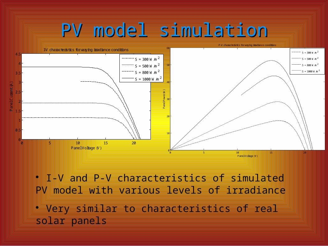
I-V characteristics for varying irradiance conditions

S = 300 W/m2

S = 500 W/m2

S = 800 W/m2

S = 1000 W/m2

0 5 10 15 200

10

20

30

40

50

60

Panel Voltage (V)

Pan

el P

ower

(W

)

P-V characteristics for varying irradiance conditions

S = 300 W/m2

S = 500 W/m2

S = 800 W/m2

S = 1000 W/m2

I-V and P-V characteristics of simulated PV model with various levels of irradiance

Very similar to characteristics of real solar panels

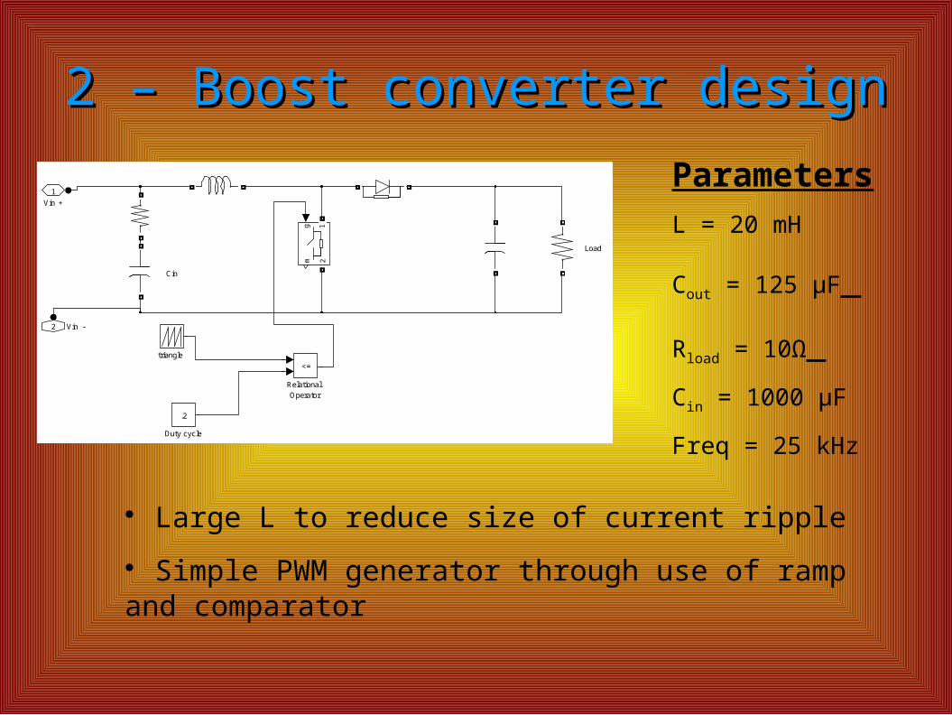
2 – Boost converter design2 – Boost converter design

Load

Cin

Vin -2

Vin +

1

triangle

RelationalOperator

<=

gm

12

Duty cycle

.2

ParametersL = 20 mH

Cout = 125 μF

Rload = 10Ω Cin = 1000 μF

Freq = 25 kHz

Large L to reduce size of current ripple

Simple PWM generator through use of ramp and comparator

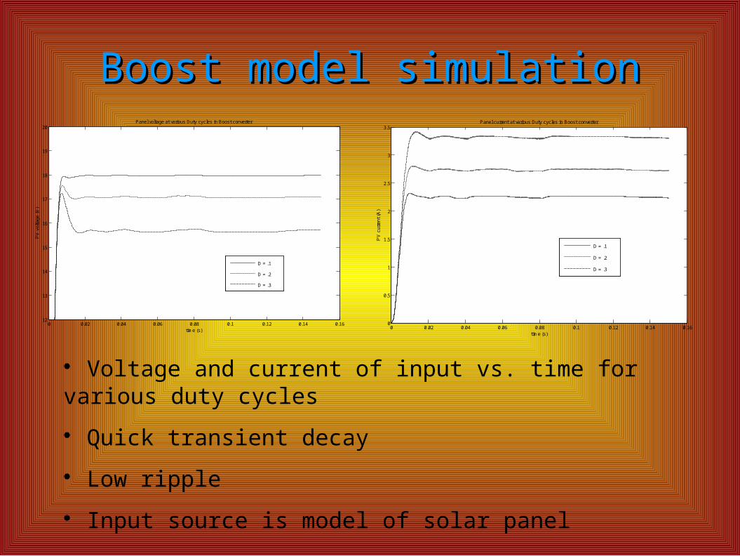
Boost model simulationBoost model simulation

0 0.02 0.04 0.06 0.08 0.1 0.12 0.14 0.160

0.5

1

1.5

2

2.5

3

3.5

time (s)

PV

cur

rent

(A

)

Panel current at various Duty cycles in Boost converter

D = .1

D = .2

D = .3

0 0.02 0.04 0.06 0.08 0.1 0.12 0.14 0.1612

13

14

15

16

17

18

19

20

time (s)

PV

vol

tage

(V

)

Panel voltage at various Duty cycles in Boost converter

D = .1

D = .2

D = .3

Voltage and current of input vs. time for various duty cycles

Quick transient decay

Low ripple

Input source is model of solar panel

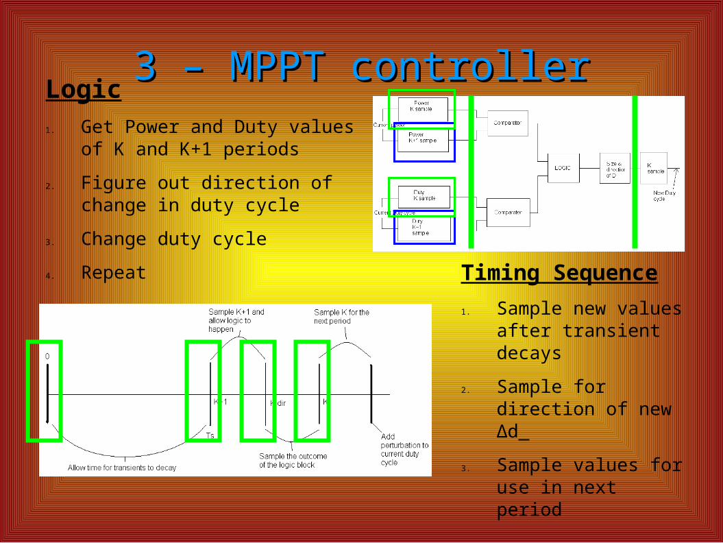
3 – MPPT controller3 – MPPT controller

Timing Sequence

1. Sample new values after transient decays

2. Sample for direction of new Δd

3. Sample values for use in next period

4. Make change in Δd

Logic1. Get Power and Duty values of

K and K+1 periods

2. Figure out direction of change in duty cycle

3. Change duty cycle

4. Repeat

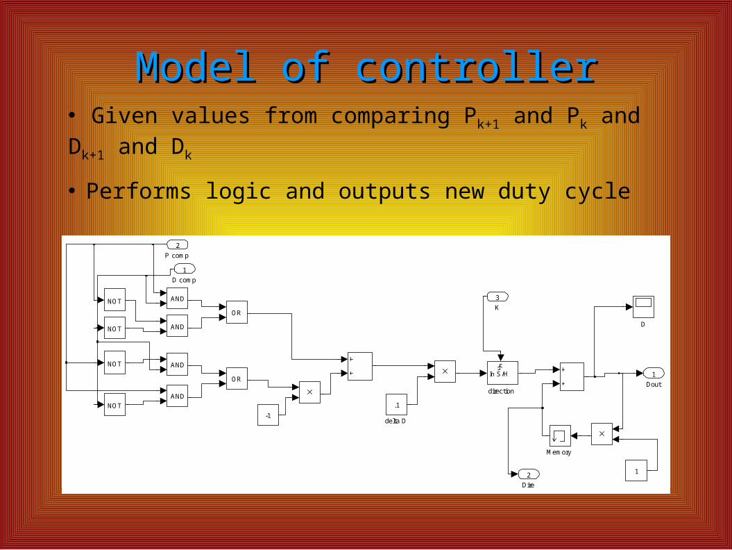
Model of controllerModel of controller

Dire

2

Dout

1

direction

In S/H

1

delta D

.1

Memory

OR

ANDNOT

ANDNOT

NOT

NOT AND

OR

AND

D

-1

K

3

P comp

2

D comp

1

Given values from comparing Pk+1 and Pk and Dk+1 and Dk

Performs logic and outputs new duty cycle

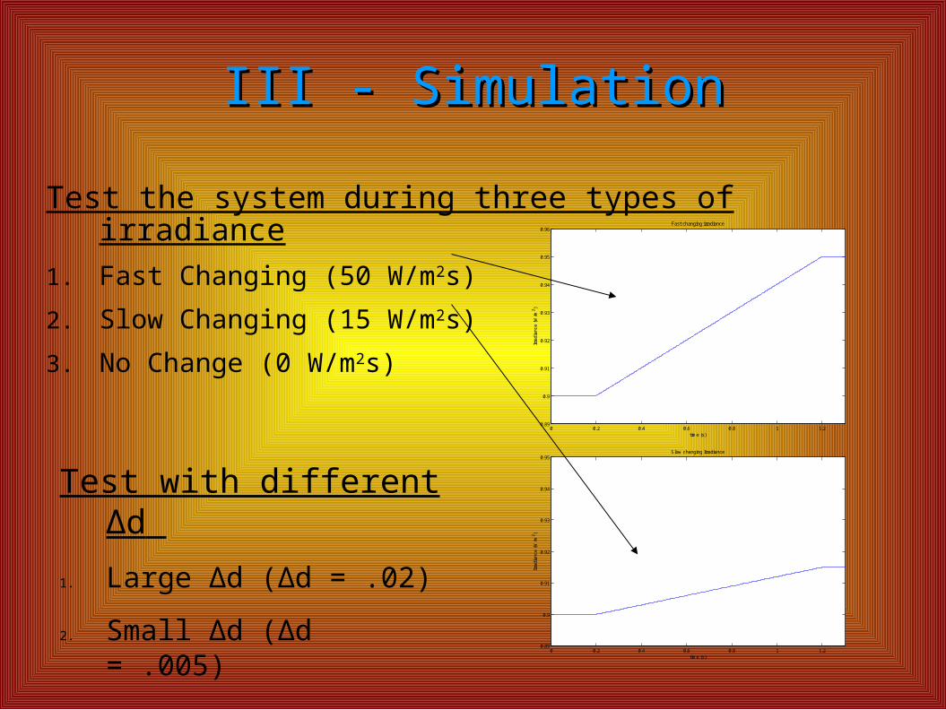
III - SimulationIII - Simulation

Test the system during three types of irradiance

1. Fast Changing (50 W/m2s)

2. Slow Changing (15 W/m2s)

3. No Change (0 W/m2s)

Test with different Δd

1. Large Δd (Δd = .02)

2. Small Δd (Δd = .005)

0 0.2 0.4 0.6 0.8 1 1.20.89

0.9

0.91

0.92

0.93

0.94

0.95

0.96

time (s)

Irra

dian

ce (

W/m

2 )

Fast changing irradiance

0 0.2 0.4 0.6 0.8 1 1.20.89

0.9

0.91

0.92

0.93

0.94

0.95

time (s)

Irra

dian

ce (

W/m

2 )

Slow changing Irradiance

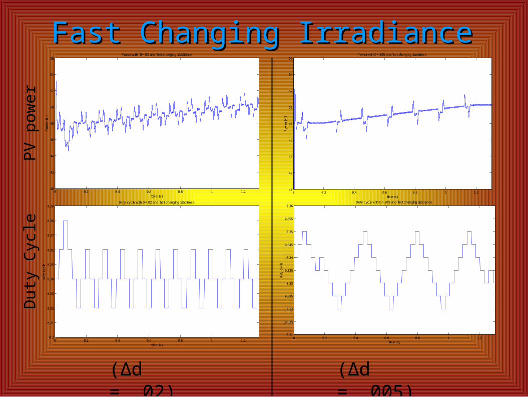
Fast Changing IrradianceFast Changing Irradiance

0 0.2 0.4 0.6 0.8 1 1.240

42

44

46

48

50

52

54

56

time (s)

Pow

er (

W)

Power with D=.02 and fast changing irradiance

0 0.2 0.4 0.6 0.8 1 1.20.3

0.31

0.32

0.33

0.34

0.35

0.36

0.37

0.38

0.39

time (s)

duty

cyc

le

Duty cycle with D=.02 and fast changing irradiance

(Δd = .02)

0 0.2 0.4 0.6 0.8 1 1.240

42

44

46

48

50

52

54

56

time (s)

Pow

er (

W)

Power with D=.005 and fast changing irradiance

0 0.2 0.4 0.6 0.8 1 1.20.31

0.315

0.32

0.325

0.33

0.335

0.34

0.345

0.35

0.355

0.36

time (s)

duty

cyc

le

Duty cycle with D=.005 and fast changing irradiance

(Δd = .005)

PV

pow

er

Du

ty C

ycl

e

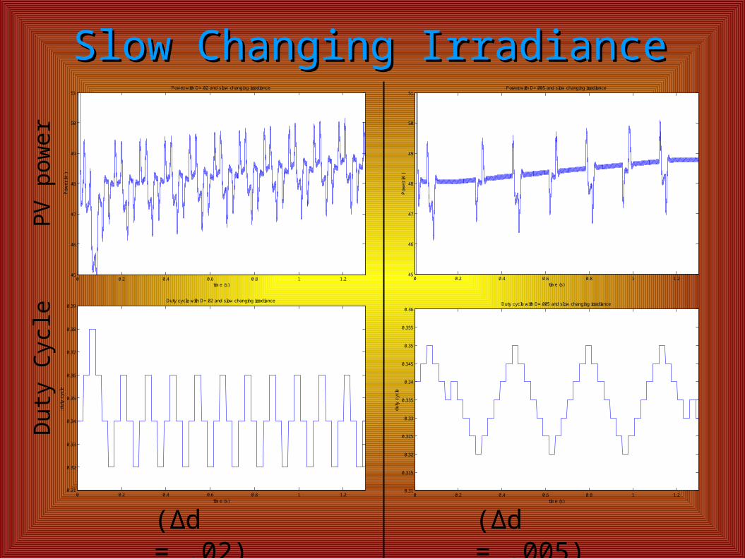
Slow Changing IrradianceSlow Changing Irradiance

(Δd = .02) (Δd = .005)

PV

pow

er

Du

ty C

ycl

e

0 0.2 0.4 0.6 0.8 1 1.20.31

0.32

0.33

0.34

0.35

0.36

0.37

0.38

0.39

time (s)

duty

cyc

le

Duty cycle with D=.02 and slow changing irradiance

0 0.2 0.4 0.6 0.8 1 1.245

46

47

48

49

50

51

time (s)

Pow

er (

W)

Power with D=.005 and slow changing irradiance

0 0.2 0.4 0.6 0.8 1 1.20.31

0.315

0.32

0.325

0.33

0.335

0.34

0.345

0.35

0.355

0.36

time (s)

duty

cyc

le

Duty cycle with D=.005 and slow changing irradiance

0 0.2 0.4 0.6 0.8 1 1.245

46

47

48

49

50

51

time (s)

Pow

er

(W)

Power with D=.02 and slow changing irradiance

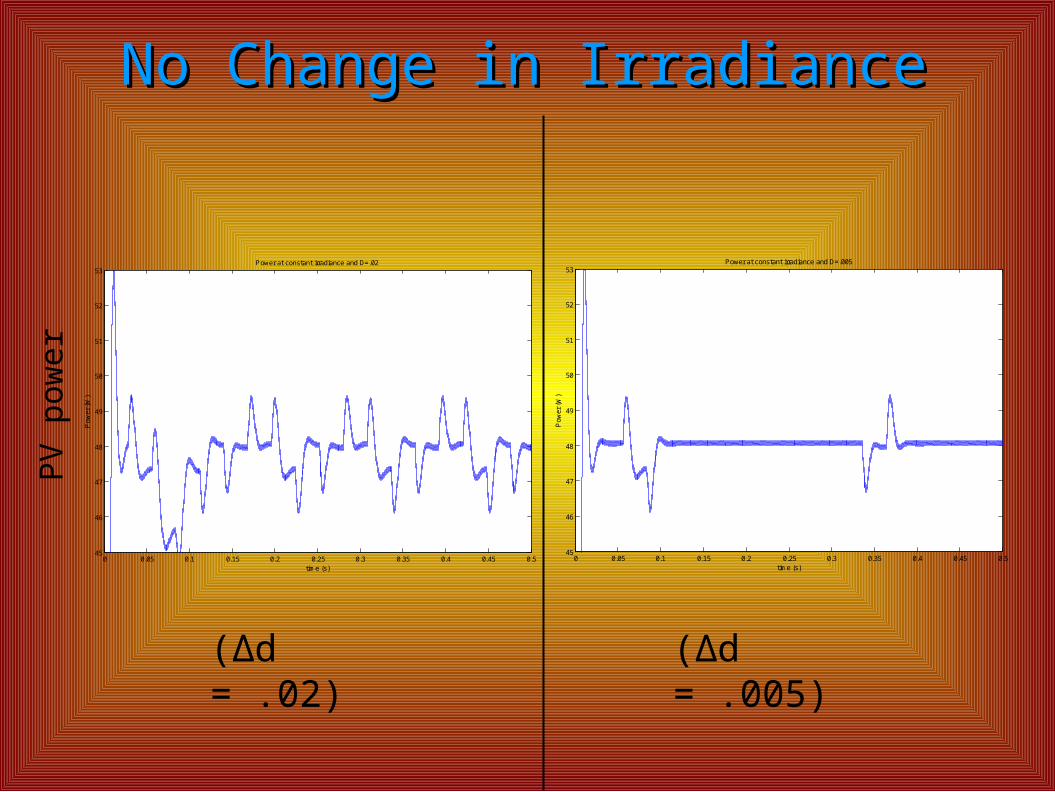
No Change in IrradianceNo Change in Irradiance

(Δd = .02) (Δd = .005)

PV

pow

er

0 0.05 0.1 0.15 0.2 0.25 0.3 0.35 0.4 0.45 0.545

46

47

48

49

50

51

52

53

time (s)

Pow

er (

W)

Power at constant irradiance and D=.02

0 0.05 0.1 0.15 0.2 0.25 0.3 0.35 0.4 0.45 0.545

46

47

48

49

50

51

52

53

time (s)

Pow

er (

W)

Power at constant irradiance and D=.005

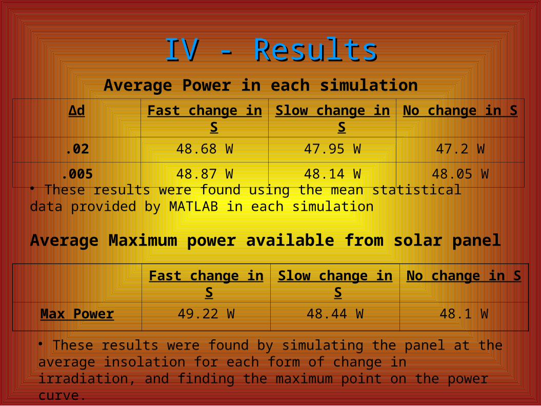
IV - ResultsIV - Results

Δd Fast change in S Slow change in S No change in S

.02 48.68 W 47.95 W 47.2 W

.005 48.87 W 48.14 W 48.05 W

Average Power in each simulation

These results were found using the mean statistical data provided by MATLAB in each simulation

Average Maximum power available from solar panel

Fast change in S Slow change in S No change in S

Max Power 49.22 W 48.44 W 48.1 W

These results were found by simulating the panel at the average insolation for each form of change in irradiation, and finding the maximum point on the power curve.

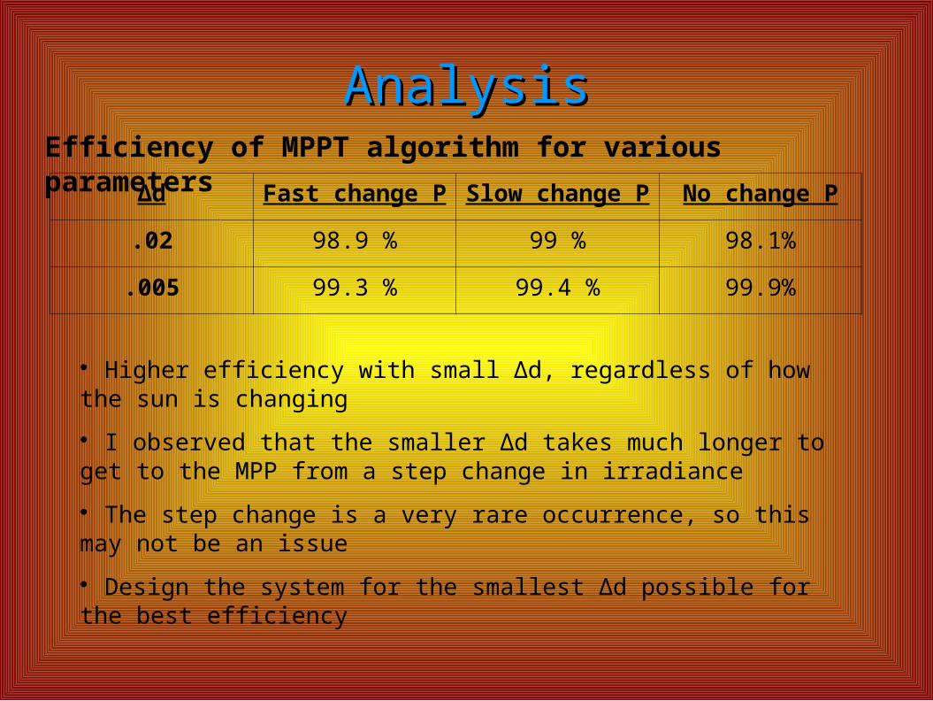
AnalysisAnalysis

Δd Fast change P Slow change P No change P

.02 98.9 % 99 % 98.1%

.005 99.3 % 99.4 % 99.9%

Efficiency of MPPT algorithm for various parameters

Higher efficiency with small Δd, regardless of how the sun is changing

I observed that the smaller Δd takes much longer to get to the MPP from a step change in irradiance

The step change is a very rare occurrence, so this may not be an issue

Design the system for the smallest Δd possible for the best efficiency

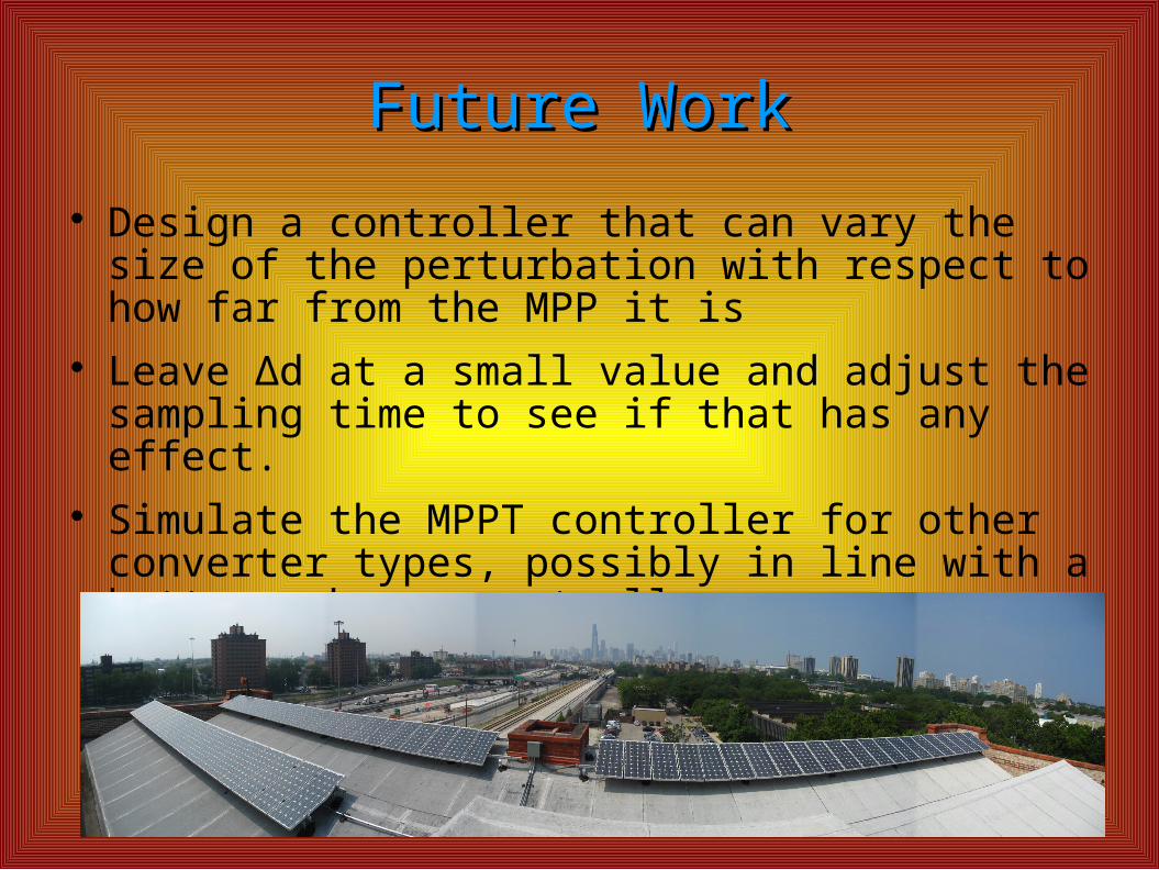
Future WorkFuture Work

Design a controller that can vary the size of the perturbation with respect to how far from the MPP it is

Leave Δd at a small value and adjust the sampling time to see if that has any effect.

Simulate the MPPT controller for other converter types, possibly in line with a battery charge controller