Solar Irradiance Curves, Cirrus Contamination, and Sun Glint

Bo-Cai Gao1, Rong-Rong Li1, David Thompson2, and Robert O. Green2

June 2014

1Remote Sensing Division, Naval Research Laboratory, Washington, DC2Jet Propulsion Lab, California Institute of Technology, Pasadena, CA

INTRODUCTION

• Solar irradiance curves – In the mid-1990s, we started to question the

validity of the 1985 standard solar irradiance curve by C. Wehrli of World

Radiation Center in Switzerland. A paper on the subject was published in

1996 (Applied Optics)

• Cirrus contamination – We began to address the cirrus detection and

correction issue in early 1990s.

• Sun glint – By analyzing the AVIRIS data acquired over Salton Sea in

California in the summer of 1988, we realized that the sunglint effects in

the 0.4 – 2.5 micron wavelength range are spectrally flat, and the sunglint

effects should, in principle, be correctable.

2

Relevant Equations and Definitions

In the absence of gas absorption, the radiance at the satellite level is:

L*obs = L*0 + Lg t'u + Lw tu, (1)

L*0: path radiance; Lw: water leaving radiance;

Lg: radiance reflected at water surface; t’u & tu: upward transmittances

Multiply Eq. (1) by p and divide by (m0 E0), Eq. (1) becomes:

p Lobs / (m0 E0) = p L*0 / (m0 E0) + p Lg t'u [td / (m0 E0 td ) ]

+ p Lw tu [td / (m0 E0 td )] (2)

where E0 = solar irr., m0 = cosine of solar zenith angle. We define:

Satellite apparent reflectance: r*obs = p Lobs / (m0 E0), (3)

r*atm = p L*0 / (m0 E0), (4)

Glint reflectance: rg = p Lg / (m0 E0 td ) (5)

Water leaving reflectance: rw = p Lw / (m0 E0 td ) = p Lw / Ed (6)

Remote sensing reflectance: Rrs = rw / p = Lw / Ed (6’)

Substitute Eqs (3) – (6) into Eq. (2), we get:

r*obs = r*atm + rg td tu + rw td tu (7)

After consideration of gas absorption and multiple reflection between the

atmosphere and surface, & denoting r*atm+glint = r*atm + rg td tu, we can get:

rw = (r*obs/Tg - r*

atm+glint) / [td tu + s (r*obs/Tg - r*

atm+glint) ] (8)

Gao, B.-C., M. J. Montes, Z. Ahmad, and C. O. Davis, Appl. Opt., 39, 887-896, February 2000.

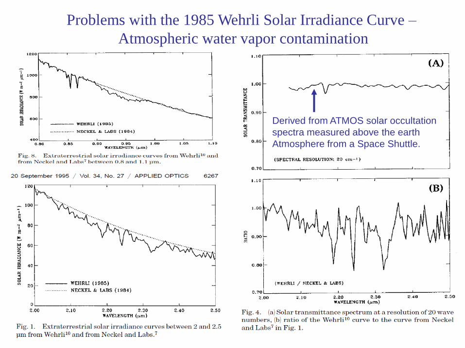
Problems with the 1985 Wehrli Solar Irradiance Curve –

Atmospheric water vapor contamination

Derived from ATMOS solar occultation

spectra measured above the earth

Atmosphere from a Space Shuttle.

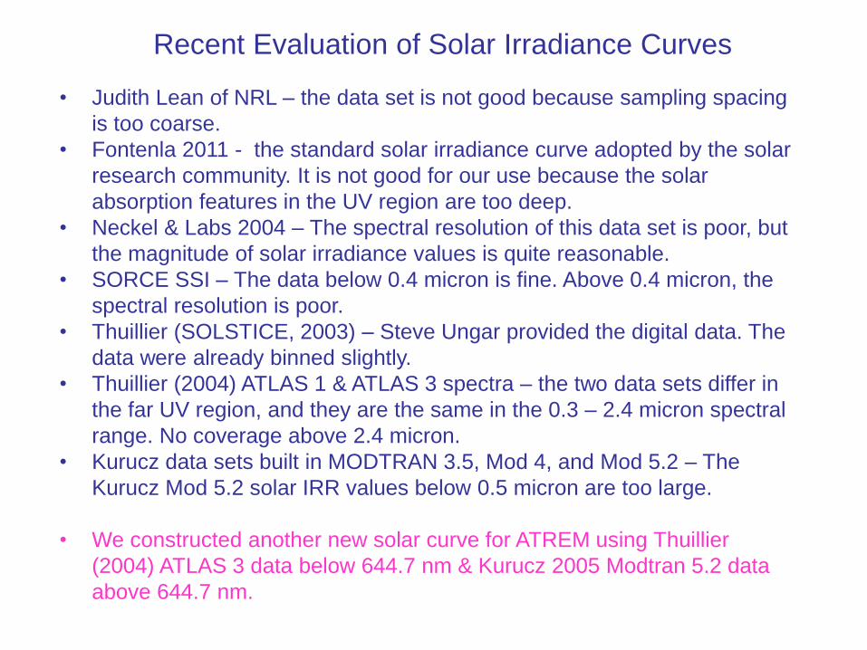
Recent Evaluation of Solar Irradiance Curves

• Judith Lean of NRL – the data set is not good because sampling spacing

is too coarse.

• Fontenla 2011 - the standard solar irradiance curve adopted by the solar

research community. It is not good for our use because the solar

absorption features in the UV region are too deep.

• Neckel & Labs 2004 – The spectral resolution of this data set is poor, but

the magnitude of solar irradiance values is quite reasonable.

• SORCE SSI – The data below 0.4 micron is fine. Above 0.4 micron, the

spectral resolution is poor.

• Thuillier (SOLSTICE, 2003) – Steve Ungar provided the digital data. The

data were already binned slightly.

• Thuillier (2004) ATLAS 1 & ATLAS 3 spectra – the two data sets differ in

the far UV region, and they are the same in the 0.3 – 2.4 micron spectral

range. No coverage above 2.4 micron.

• Kurucz data sets built in MODTRAN 3.5, Mod 4, and Mod 5.2 – The

Kurucz Mod 5.2 solar IRR values below 0.5 micron are too large.

• We constructed another new solar curve for ATREM using Thuillier

(2004) ATLAS 3 data below 644.7 nm & Kurucz 2005 Modtran 5.2 data

above 644.7 nm.

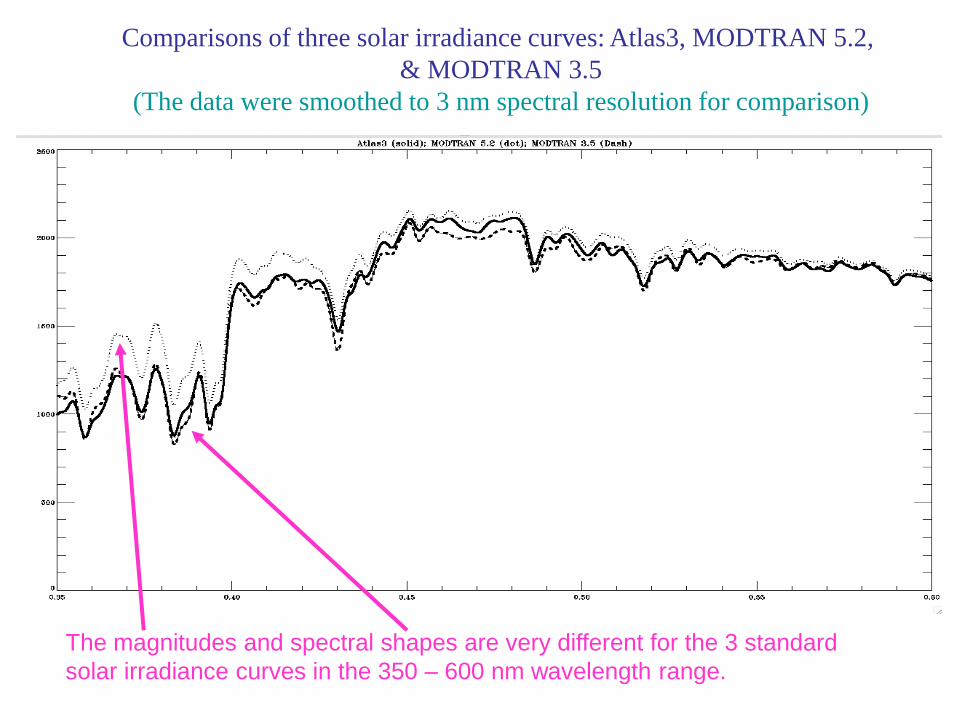
Comparisons of three solar irradiance curves: Atlas3, MODTRAN 5.2,

& MODTRAN 3.5

(The data were smoothed to 3 nm spectral resolution for comparison)

The magnitudes and spectral shapes are very different for the 3 standard

solar irradiance curves in the 350 – 600 nm wavelength range.

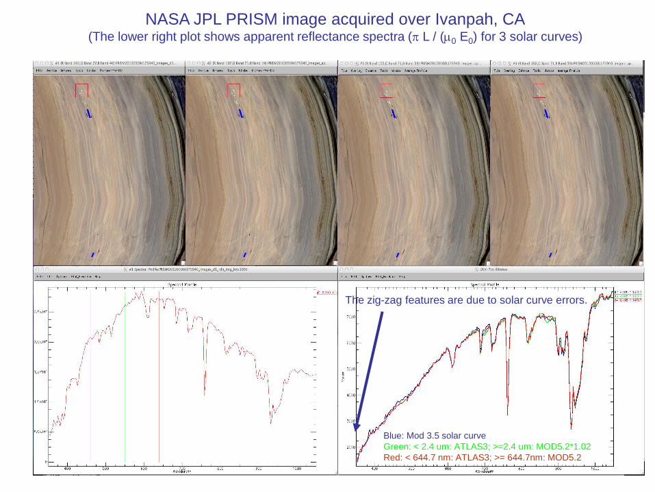
Blue: Mod 3.5 solar curve

Green: < 2.4 um: ATLAS3; >=2.4 um: MOD5.2*1.02

Red: < 644.7 nm: ATLAS3; >= 644.7nm: MOD5.2

NASA JPL PRISM image acquired over Ivanpah, CA(The lower right plot shows apparent reflectance spectra (p L / (m0 E0) for 3 solar curves)

The zig-zag features are due to solar curve errors.

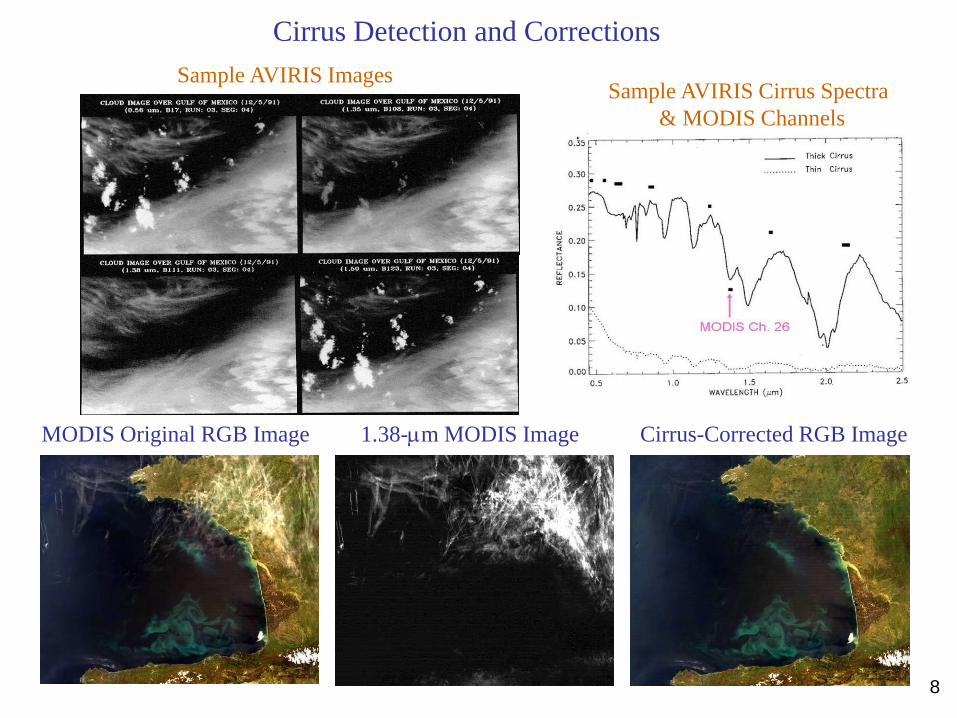
MODIS Original RGB Image 1.38-mm MODIS Image Cirrus-Corrected RGB Image

Cirrus Detection and Corrections

Sample AVIRIS ImagesSample AVIRIS Cirrus Spectra

& MODIS Channels

8

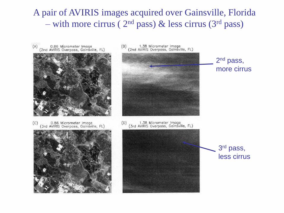
A pair of AVIRIS images acquired over Gainsville, Florida

– with more cirrus ( 2nd pass) & less cirrus (3rd pass)

2nd pass,

more cirrus

3rd pass,

less cirrus

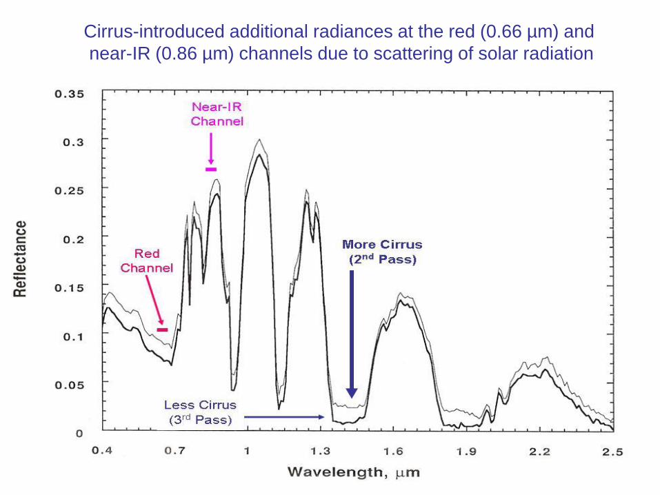
Cirrus-introduced additional radiances at the red (0.66 µm) and

near-IR (0.86 µm) channels due to scattering of solar radiation

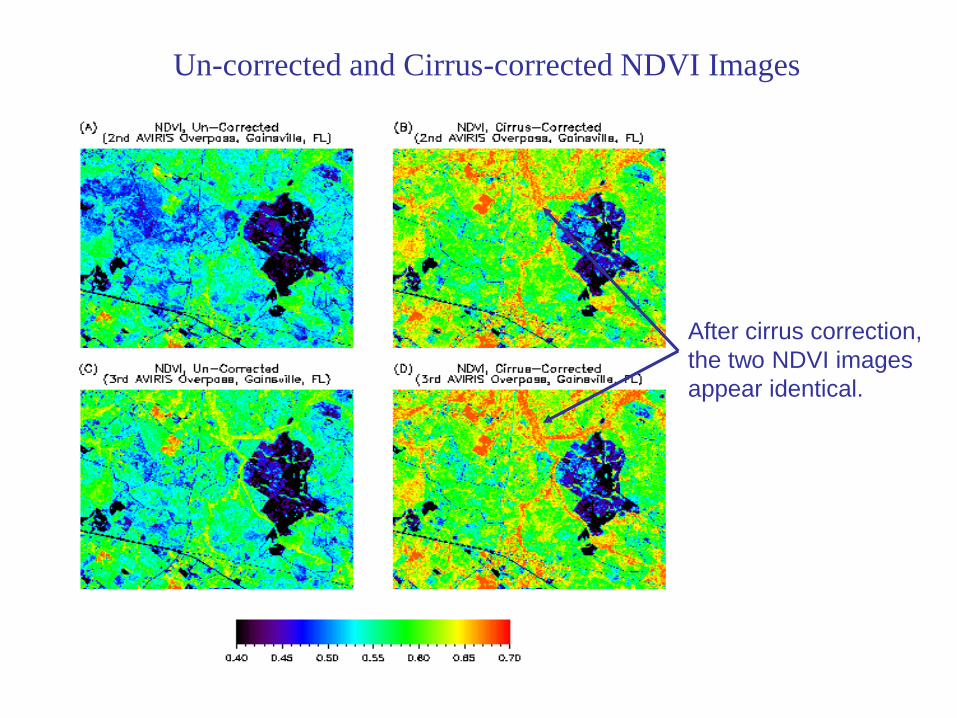
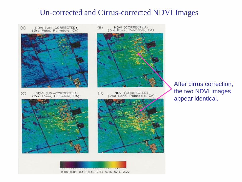
Un-corrected and Cirrus-corrected NDVI Images

After cirrus correction,

the two NDVI images

appear identical.

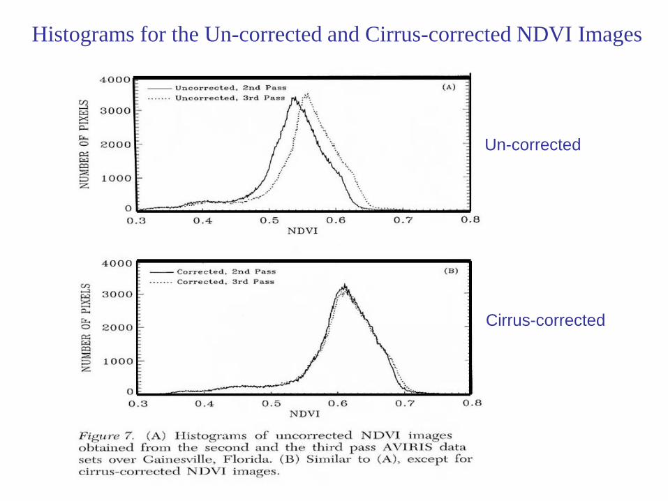
Histograms for the Un-corrected and Cirrus-corrected NDVI Images

Un-corrected

Cirrus-corrected

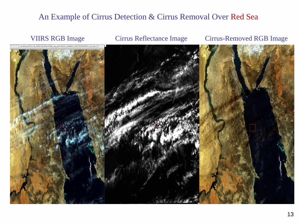
An Example of Cirrus Detection & Cirrus Removal Over Red Sea

VIIRS RGB Image Cirrus-Removed RGB ImageCirrus Reflectance Image

13

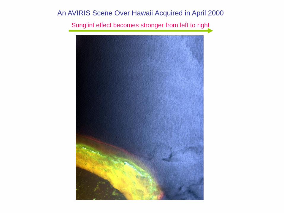
An AVIRIS Scene Over Hawaii Acquired in April 2000

Sunglint effect becomes stronger from left to right

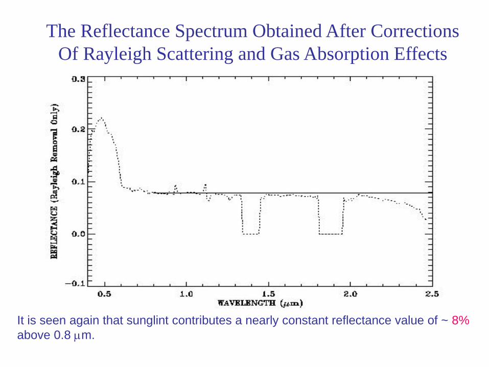
The Reflectance Spectrum Obtained After Corrections

Of Rayleigh Scattering and Gas Absorption Effects

It is seen again that sunglint contributes a nearly constant reflectance value of ~ 8%

above 0.8 mm.

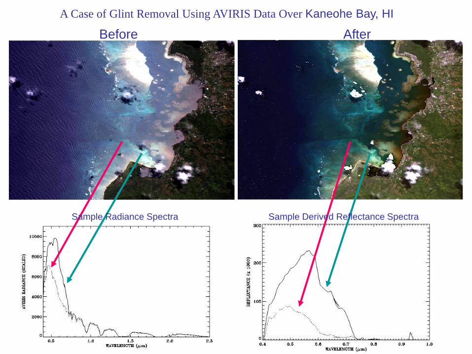
A Case of Glint Removal Using AVIRIS Data Over Kaneohe Bay, HI

Before After

Sample Derived Reflectance SpectraSample Radiance Spectra

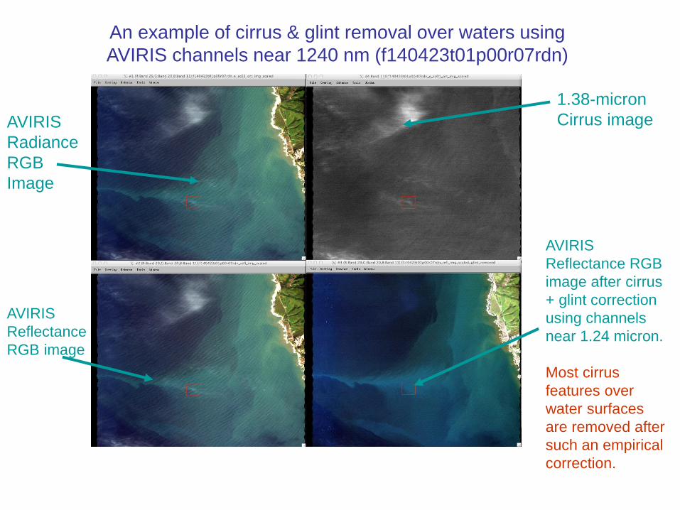
An example of cirrus & glint removal over waters using

AVIRIS channels near 1240 nm (f140423t01p00r07rdn)

AVIRIS

Radiance

RGB

Image

1.38-micron

Cirrus image

AVIRIS

Reflectance

RGB image

AVIRIS

Reflectance RGB

image after cirrus

+ glint correction

using channels

near 1.24 micron.

Most cirrus

features over

water surfaces

are removed after

such an empirical

correction.

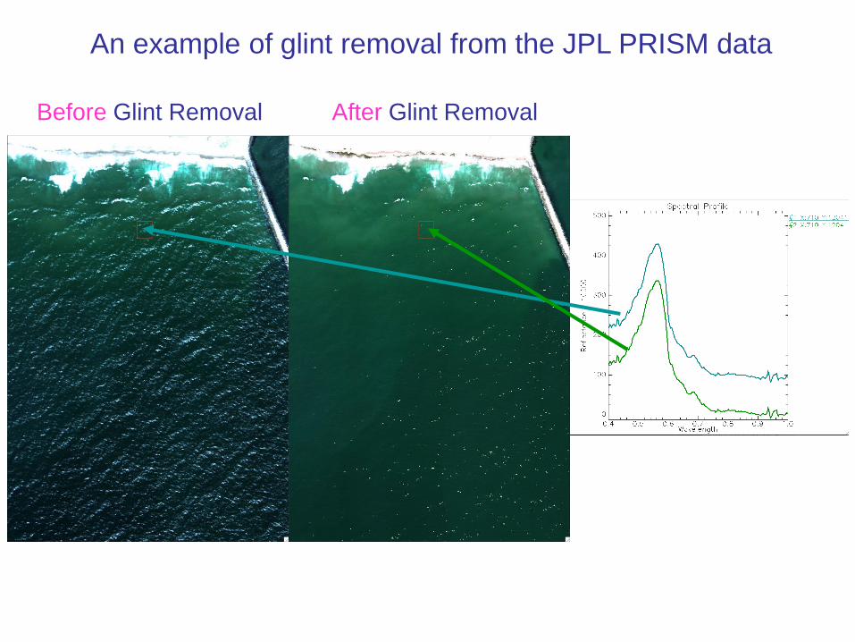
An example of glint removal from the JPL PRISM data

Before Glint Removal After Glint Removal

SUMMARY

• In this presentation, I have covered three topics – solar irradiance curves,

cirrus detection and corrections, and empirical glint removal.

• For proper retrieval of land surface reflectances and water leaving

reflectances from hyperspectral imaging data, we still need an improved

solar irradiance curve.

• So far, the empirical techniques presented here for removing thin cirrus

and sunglint effects have not been used in operational codes.

Improvements in treating the downward and upward atmospheric

transmittance terms are still needed.

Un-corrected and Cirrus-corrected NDVI Images

After cirrus correction,

the two NDVI images

appear identical.

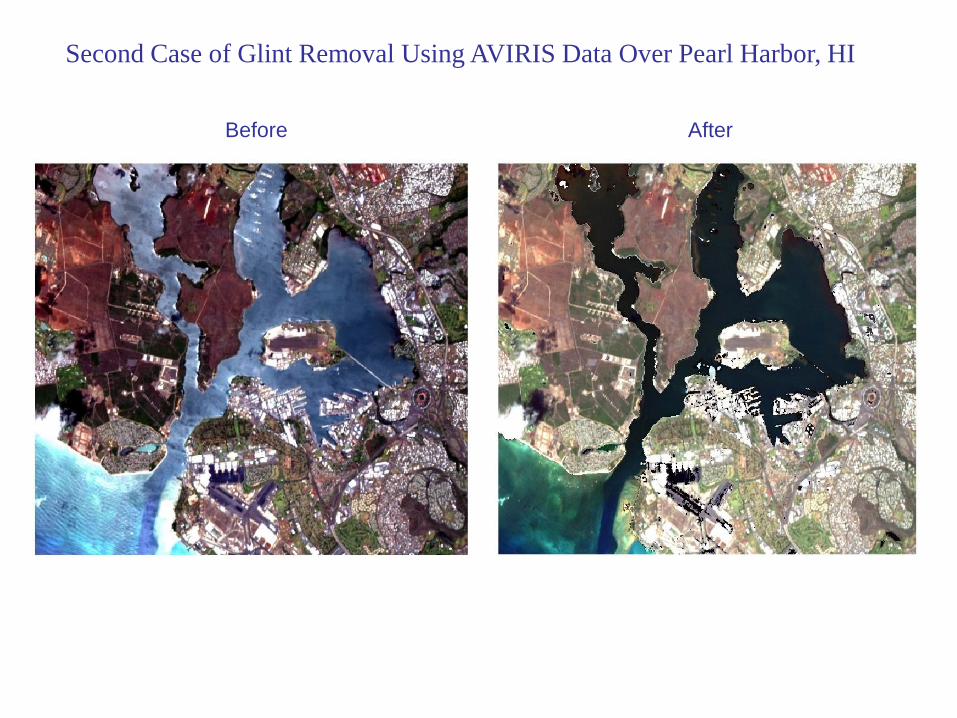
Second Case of Glint Removal Using AVIRIS Data Over Pearl Harbor, HI

Before After