Embed Size (px)
Citation preview
SOLAR ENERGY CONVERSION SYSTEMS
ENGINEERING AND ECONOMIC ANALYSIS
INPUT DEFINITION
Volume I
GILBERTO RUSSO*
prepared for the
UNITED STATES
DEPARTMENT OF ENERGY
under contractNo. EX-76-A-01-2295Task Order 37b
*on leave from the Polytechnic of Torino, Italy, Faculty of Engineering
TABLE OF CONTENTS
INTRODUCTION
1 SOLAR RADIATION
1.1 Solar Constant Computation
2 ASTRONOMICAL PARAMETERS
2.1 Sun-Earth Distance
2.2 Declination Angle
2.3 Azimuth and Altitude of the Sun
2.3.1 Altitude
2.3.2 Azimuth
2.4 Daytime
2.5 Zenith Angle
2.6 Examples
2.6.1 Declination Angle Computation
2.6.2 Solar Altitude Computation
2.6.3 Solar Azimuth Computation
2.6.4 Geometrical Daylength Computation
2.6.5 Problems
3 INTERACTION OF THE SOLAR RADIATION WITH THEATMOSPHERE
3.1 Radiation Absorption in the Atmosphere
Page
1
14
15
19
19
20
21
22
23
24
26
27
28
29
30
32
33
44
45
Page
3.1.1 The Absorption Spectrum of WaterVapor and Water 48
3.1.2 The Absorption Spectrum of Ozoneand Oxygen 51
3.1.3 The Absorption Spectrum of MinorRadiation-Absorbing AtmosphericConstituents 52
3.2 Radiation Scattering in the Atmosphere 53
4 SOLAR ENERGY RADIATIVE FLUX DEPLETION 60
4.1 Optical Depth for a Vertical Path 62
4.2 Atmospheric Mass: Optical Depth for anArbitrary Inclined Path 66
4.3 Integral Transmission Factor of theAtmosphere 75
4.4 Attenuation of Solar Radiation by Clouds 79
5 CORRELATION OF THE SOLAR ENERGY RADIATIVE FLUXDEPLETION WITH METEOROLOGICAL CONDITIONS 89
5.1 Depletion "Constant" of the Atmosphere 91
5.1.1 Macroclimatic Approximation 91
5.1.2 Microclimatic Approximation 98
5.2 Quantitative Aspects of the Cloud Presence 130
5.2.1 Macroclimatic Approximation 130
5.2.2 Microclimatic Approximation 131
5.3 Solmet - Meteorological Data 134
5.4 Summary and Model Input Data 138
5.4.1 Energy Flux Density in a ClearAtmosphere (No Clouds) 138
5.4.2 Energy Flux Density for anAtmosphere with Clouds
5.4.3 Energy Flux
APPENDIX Al: IRRADIANCE:MEASURE
DEFINITIONS AND UNITS OF
1 Units of Measure
1.1 Radiometric Scale (S.I. Units)
1.2 Photometric Scale
2 Definitions
APPENDIX A2: RADIATION LAWS APPLIED TO COMPUTATIONOF SOLAR ENERGY FLUXES
1 Lambert's Law
2 Stefan-Boltzmann's Law
3 Kirchoff's Law
4.1 First Wien's Law
4.2 Second Wien's Law
5 Planck's Law
APPENDIX A3: COMPUTATION OF THE AMOUNT OF PRECIPITABLEWATER AND OF THE EQUIVALENT HEIGHT OF THEATMOSPHERE
1 Precipitable Water Computation
2 Equivalent Height Computation
APPENDIX A4: INSOLATION CLIMATOLOGY DATA ON SOLMETFORMAT
Page
140
141
144
144
145
146
148
150
150
151
151
152
153
153
155
161
171
179
APPENDIX A5: W.M.O. CLOUD DEFINITION ANDCLASSIFICATION
1 Cloud Classification
2 Cloud Definition
APPENDIX A6: ANALOGIC RECORDS OF SURFACE WEATHEROBSERVATION
CONVERSION TABLE
NOMENCLATURE
REFERENCES
Page
187
187
189
193
196
200
205
ABSTRACT
After defining Solar Energy Conversion System Input
characteristics, an analytical model of the atmosphere is
developed. This model is capable of computing the Solar Energy
Flux on the collector area for a techno-economic feasibility
analysis of Solar Energy Systems.
A deterministic approach permits the evaluation of the
energy input to the system, at proper intervals of time, on
the basis of a few meteorological data. The selective inter-
action of the electromagnetic energy flux and atmospheric
matter is described: the analytical model is derived and imple-
mented on CIRR2 codes for the global energy flux computation;
and comparison with experimental values is performed.
INTRODUCTION
"Felix qui potuit rerum cognoscere causas"
Virgil, Georg.: II 490
Energy Conversion Systems engineering may be considered as
an interface between the energy load and the energy input. Upon
definition of the energy load, Primary Energy Conversion Systems
are engineered on the basis of an energy input that may be con-
sidered available any time at the desired intensity: this allows
a quasi-steady state mode of operation of the system (and of the
components) and reduces the excursion of the design parameters
during operation. Solar Energy Conversion Systems must be
designed taking into account a highly variable energy input to
the system; they therefore operate in non-steady state condi-
tions that strongly affect the performances of the system and
the energy output itself. Consequently, economic evaluations
of the system should take into account the transient mode of
operation of the system.
Therefore, Solar Energy Conversion Systems engineering
optimization, economic analysis and those energy strategies
that strongly consider them, heavily rely on an adequate know-
ledge of the energy input to the system, i.e. on an adequate
1
knowledge of the solar energy radiative flux on the collector
area, both for system and components' analysis.
The quantity and reliability of experimental data available
in the U.S. are discussed on Chapter 5 and Appendices A4 and A6.
As will be shown, the availability, quality and quantity of the
data will sensibly improve the standardization of instruments,
number of stations, etc. being improved. The present situation,
however, is somewhat more critical. Besides,the availability
of the data for most other countries of the world, as concerns
energy flux values, is particularly poor and the information
unreliable, although these countries represent a highly attrac-
tive potential market.
The alternative to using experimental data is to compute
them. A stochastic or a deterministic approach may be used.
The former may be performed with regression models, e.g. through
correlation of the various radiative components of the radiation
flux or through Monte Carlo methods, but generally obtained
through largely macroclimatic correlations using empirical
algorithms or through time-consuming large-scale meteo-atmos-
pheric models. The criteria adopted in this work are the
construction of an ahalytical model of the atmosphere on the
basis of a reduced number of "generally" available meteorologi-
cal parameters (i.e., parameters already available through
standard measurements), giving to the analytical model the
2
characteristics of a physical model of the atmosphere rather
than a mathematical algorithm of correlation, with a relative
low time of computation.
This solution is consistent with the engineering of the
system due to the fact that many aspects of this engineering
(for components and systems) are achieved via computer (due to
the large time-dependent number of variables), and optimization
techniques and techno-economical feasibility analysis are imple-
mented through computer models. It is attractive because of the
worldwide dearth of solar energy flux data (but not of some
standard meteorological measurements, such as pressure, tempera-
ture, relative humidity, etc.). The last point is particularly
important. The measurement of most meteorological parameters
is standardized; the instrumentation and techniques of measure-
ments are simple and economical; a considerable amount of
historical data are available; meteorological parameters do
not change as rapidly--step function--as solar energy fluxes,
and therefore a relatively reduced number of measurements would
allow the computation, even on a minute basis, of the solar
energy flux. The only exception to this are clouds, but their
presence may be simulated with a stochastic approach without
losing much precision and without losing information on the
gradients of solar energy flux values. Besides, some informa-
tion on clouds is generally available, in that they are an
important component in determining the radiative equilibrium
of the Earth. This information permits a day-to-day match of
3
solar energy flux density with, for instance, experimental values.
This is of paramount importance for load profiles (e.g., analysis
of the homeostasis of electrical energy obtained through solar
energy conversion with the utilities grid).
This approach has been chosen because it appears that an
analytical model of the atmosphere may be realized, up to a
certain degree of precision, using available standard meteoro-
logical measurements. Its precision appears to be comparable
to the precision (or anyhow to the real information content)
of the solar energy flux measurements (obviously affected by
errors and "local" effects that distort their real information
content). An increase in precision of the physical model is
theoretically possible, but it would then be problematic to find
the necessary input data, i.e., the phenomena involved in the
selective interaction of electromagnetic solar flux and the
components of the atmosphere may be described, in a relatively
simple way, by the classic-physics approach, but the informa-
tion needed to perform the calculation (information on the
atmospheric system) is not available.
This same concept of information content approach has
eliminated the regression models, e.g., computing the direct
component of this energy flux from its global component or
computing historical data from actual data.
Another reason why this approach has been used is that
our purpose is to obtain a day-to-day (or hour-to-hour) match
4
of computed to experimental data, as has been shown previously
with the homeostasis example. That is, we are mainly interested
in a deterministic approach; this is why other powerful stochastic
(non-deterministic) approaches, although considered, have been
abandoned (e.g., Monte Carlo methods).
The analytical model should therefore behave as a "transfer
function: for the "normalization" of the solar energy input.
The solar energy radiative characteristics are presented
in Chapter 1 and radiation laws are recalled in Appendix Al;
the computation of astronomical parameters is performed in
Chapter 2; the selective interaction between the electromagnetic
energy and the components of the atmosphere is discussed in
Chapter 3; the solar energy flux depletion model is presented
in Chapter 4, where the mathematical algorithm is developed;
the correlation of the energy flux depletion to the meteorologi-
cal parameters (on a macro- and micro-climatic approximation)
and the analysis of the meteorological input data (as well as
alternative ways of computing some of the input data) are per-
formed in Chapter 5 and Appendices A2, A3, A4, A5, and A6.
Chapter 6 (in Volume II) contains the implementation
criteria of the global energy flux model. The characteristics
of the CIRR2 code obtained upon implementation of the analytical
model are reported in Appendix A7 (Volume II); the analysis of
5
the final results and samples of output information are reported
in Chapter 7 (Volume II). Direct and diffuse components compu-
tation will be performed in Volume III.
Finally, Volume IV will report overall analysis performed
with CIRR's codes (all related to the input definition).
It should be noted that the input definition of Solar
Energy Conversion Systems is viewed as an introduction and not
as a conclusion to this work, which aims to develop a techno-
economical feasibility and optimization analysis.
Therefore, the main criteria of development of the analy-
tical model of the atmosphere are related to the fact that, due
to the characterization of Solar Energy Conversion Systems,
with respect to Primary Energy Conversion Systems, the solar
energy input should be known following certain requirements.
It has been briefly shown how those requirements are satisfied
by the approach chosen. It would be proper, for the future
development of the work, to stress the real content of those
requirements, which follows directly from the characteristics
of the Solar Energy Conversion Systems. Those characteristics
become evident from a rigorous definition of Solar Energy Con-
version Systems. The next paragraphs will be devoted to this
task.
6
Any Energy Conversion System--including one-component
systems--that has a partial or total energy input solar energy
radiative flux, on either a passive or an active component, is
here defined as a Solar Energy Conversion System. A further
condition, imposed on the output of the energy conversion
system, is that the output supplies a load that, independent of
its entity or entropy content, would otherwise be covered by
primary energy--i.e., energy available through conversion of
natural high-available-energy "fuels"--or would not be covered
at all. This is the definition that will be used in the fol-
lowing volumes, when performing the techno-economical feasibility
analysis.
Many differentiations among Solar Energy Conversion
Systems have been proposed and adopted, depending on the type
of analysis performed either on systems or components differen-
tiations, on materials technology differentiations, on the end
use of the energy converted, or on the temperature at which
this energy is available.
In this work, the definition of the different Solar Energy
Conversion Systems will be based mainly on the type of physical
phenomena involved in the conversion, or the level of availability
of the energy output and/or the type of technology employed [1].
A Solar Energy System with no machinery, i.e., no dynamic
component or dynamic artificial working fluid, whose main
7
function is to trap and not to convert the solar energy within the
system, will be defined a a Passive Solar Energy System, or as
a Solar Energy System. The component definition is implicit
above. It should be emphasized that the so-called passive sys-
tems are not considered as Solar Energy Conversion Systems, since
they do not convert or even transport energy. This is non-trivial
information, although it will be used mainly on the engineering
optimization part of this work. As concerns the input definition,
many--but not all--of the considerations that will be presented
apply to any Solar Energy System [2].
The active systems definition follows, being antithetical.
All Solar Energy Conversion Systems are active following these
criteria; therefore, we will refer to them just as Solar Energy
Conversion Systems.
A first subdivision considered is between direct and in-
direct conversion systems. The former converts the electromag-
netic flux into electrical energy with no machinery or dynamic
subsystem or component associated with the conversion phenome-
non itself (electromagnetic radiation to electrical energy).
Machinery or dynamic modules may be part of the system, though,
but are not actively involved in the energy conversion phenomenon
itself. The effect of their presence may only optimize the
engineering or economic characteristics of the system as a whole.
The latter do not convert the electromagnetic energy flux into
8
electricity satisfying the above-mentioned constraints--i.e.,
they are not based on the same physical phenomenon--or do not
convert the electromagnetic flux into electrical energy at all,
but into energy generally at lower availability levels.
The indirect energy conversion systems may have, as energy
output from the subsystem or component involved in the energy
conversion, energy at high or low availability. The threshold
between the two different levels of availability is arbitrarily
taken as the availability that would correspond to energy fur-
nished as heat at 100 C and 1 atm. of pressure, with respect
to the ambience at 20 C. This is only a reference value,
and varies, for instance, with location and period of the year.
This apparently complex definition corresponds to the differen-
tiation between low-temperature and high-temperature conversion
systems.
Those are the considerations that concern the phenomena
involved and the thermodynamics of the conversion ("physical
phenomena").
The systems may also be differentiated by their technical
or operative characteristics (concentrators or not, sun-tracking
or fixed-collector areas, etc.). Those differentiations will be
considered as second order, in the sense that all the systems
will be primarily defined in the optic previously presented [3].
9
The engineering of these Solar Energy Conversion Systems
requires the knowledge of both the values and the dynamics of
variation of the design parameters. The latter is information
of paramount importance to engineering optimization of the sys-
tem, since the components and system's design approach employed
is the classical non-steady state conditions of operation design
(transient operation mode) [4,5]. The variations caused by this
operation on some of the design variables may induce critical
conditions of system operation (when approaching a limit curve
of component operation) and strongly affects the reliability
and efficiency of the system [6].
As has already been pointed out, those characteristics of
the Solar Energy Conversion System affect not only the engineering
but also the economics of the system, and act on the overall
efficiency. They are important and should be considered in any
energy policy analysis, since they impose certain limitations
on the conversion system [7].
There is, indeed, a well-defined difference between the
traditional approach to primary energy conversion systems and
the also traditional approach to energy conversion systems,
in that the differentiation of the energy input involves a dif-
ferent mode of operation of the two systems. Therefore, the
overall performance of the Solar Energy Conversion System will
depend upon all those parameters that affect the solar energy
radiative flux [8].
10

Implications are : (i) A sensible variation in the
instantaneous efficiency of the energy conversion: operating
conditions cannot be generally identified with the optimal
conditions of operation; this introduces: (ii) A difficulty
in the optimization of the system and consequently, a greater
importance of economic factors. (iii) The necessity of an
energy storage facility. (iv) The energy input of the solar
system depends upon the site of the installation (i.e., latitude,
meteo-atmospheric conditions); therefore, the whole system's
characteristics (i.e., positioning of the collector of Sun-
tracking, temperatures, operation mode, etc.) also depends
upon the site and so does, consequently, the cost of the
energy produced.
The above mentioned "dependence factors" depend them-
selves upon a high number of variables. Hence the use of
computing programs for the simulation of operating conditions
for the correct design and optimization, and for an economic
evaluation of the system, is both suitable and recommended.
It follows, from what has been said about the design
criteria of Solar Energy Conversion Systems, that it is neces-
sary to dispose of a certain amount of (reliable) data on all
those parameters that affect the energy input to the system
(e.g., astronomical parameters related to the beam's direction,
beam, scattered, and global values of the energy fluxes on the
collector area), at every "instant," the interval of time magni-
tude being related to the time constants of the components and
11
the system and to the type of approach; it may go from minute
to hourly or daily values [2,5].
Assuming that all the "solar-related parameters," except
the solar energy radiative flux values, may be easily computed
(and have to be computed: for instance, the inclination of the
collector affects, ceteris paribus, the amount of scattered
radiation collected, at such a point that, for proper inclina-
tions and orientations and at certain regions of the globe, the
global energy collected by the fixed surface might equal the
amount of global energy collected by a Sun-tracking, concentrat-
ing collector). Let us focus our attention on the solar energy
flux values. They should be available in a digitized array form,
on the most restrictive conditions on a minute basis, in order
to constitute a proper "transfer function;" they should be
related both to a specific year (or month or day) and to a
typical (not necessarily average) year (or month or day). They
should be available for any "Standard Climatic Area" (S.C.A.)
or, considering particularly drastic microclimatic condition
differences within the S.C.A. considered, for any location.
They should be available for the entire world (both for national
reasons and for market expansion reasons).
All this implies the need to dispose of a "transfer func-
tion" for the "normalization" of the solar input, in order to
consider the engineering of the Solar Energy Conversion System
12
as an interface between the energy load and an energy input
perfectly defined, following the requirements imposed by Solar
Energy Conversion Systems themselves.
The Solar Energy flux data has been furnishedEnergy Meteorological Research and Training Site atSciences Research Center of the State University ofAlbany.
by the Solarthe AtmosphericNew York at
The meteorological data has been furnished by Mr. WilliamJ. Drewes, Meteorologist in charge of the Weather Service Fore-cast Office of N.O.A.A. at Albany, New York.
All the information related to SOLMET format, digitizedrecords has been obtained through Mr. F. Quinlan, Chief Clima-tological Analysis Division, National Climatic Center, Environ-mental Data Service, U.S. Department of Commerce.
Mr. J. McCombie, M.I.T. student, has done the computerwork; Mr. P. Heron, M.I.T. Energy Laboratory, Technical Editor/Writer, has edited the manuscript and Ms. A. Anderson has verypatiently inputted the text on our Wang Word Processor System.
The author shares the eventual merit of this work with allof these persons and organizations and gratefully acknowledgesthem.
13
CHAPTER 1
SOLAR RADIATION
The Sun's radiation covers practically the entire
electromagnetic spectrum, from X-rays and cosmic rays through
radio waves up to wavelengths of several tenths of meters. Some
of these emissions are strongly limited in time--i.e., they are
intensive only under very particular conditions--and the
spectrum in which the Sun emits its maximum energy is sensibly
more limited: an order of magnitude of variation of the
wavelength around the visible range that lies between 4000 and
7000 A.
The temperature at the center of the Sun is estimated to be
about 15 million degrees Kelvin. However, the photosphere
(having a depth of about 0.0005 solar radius), from which most
detectable radiation is emitted, has a temperature ranging from
4500 to 7500 degrees Kelvin. The effective blackbody
temperature, i.e., the temperature a perfect radiator would have
in order to irradiate the measured amount of radiation, is about
5800 degrees Kelvin [9,10,11].
14
1.1 SOLAR CONSTANT COMPUTATION
The energy balance of the Sun-Earth system, under the
hypothesis that the dynamics of energy exchange consists of one
emission and one absorbance only, is easily derived by applying
three basic laws of irradiance (see Appendix Al):
i. Stefan-Boltzmann's Law for the emission of the Sun, Ws
is:
WS = 4 R e a T [W]
where:
RS Sun's radius [m]
E = Sun's emissivity (or graybody factor)[adimensional]
a = Stefan-Boltzmann's constant [W m-2 K
TS Sun's temperature [K].
ii.
density
(1.1)
-4]
The "solar constant," i.e., the solar energy flux
outside the atmosphere, ES, is:
W/(4 -2) = R T4-2Es Ws (4 ) R S/P [W m-2] (1.2)
15
where:
p = average distance Sun-Earth between perihelion
and aphelion [m].
iii. Stefan-Boltzmann's Law for the emission of the Earth,
WE, is:
W = 4 w R2 e 4 [WI (1.3)EO E LW]
where:
RE = Earth's radius [m]
TE = Earth's temperature [K].
The energy balance of the Earth, under the above
assumption, brings to (Kirchoff's Law):
R2 T4/-2RS Ts/P = 4 TE (1.4)
Always assuming p as an average value between the
apihelion and the perihelion of the Earth's orbit, , and
TE = 288 degrees Kelvin [12], from eq. 1.4 we obtain for TS a
value very close to 5900 degrees Kelvin. Hence, from eq. 1.2:
16
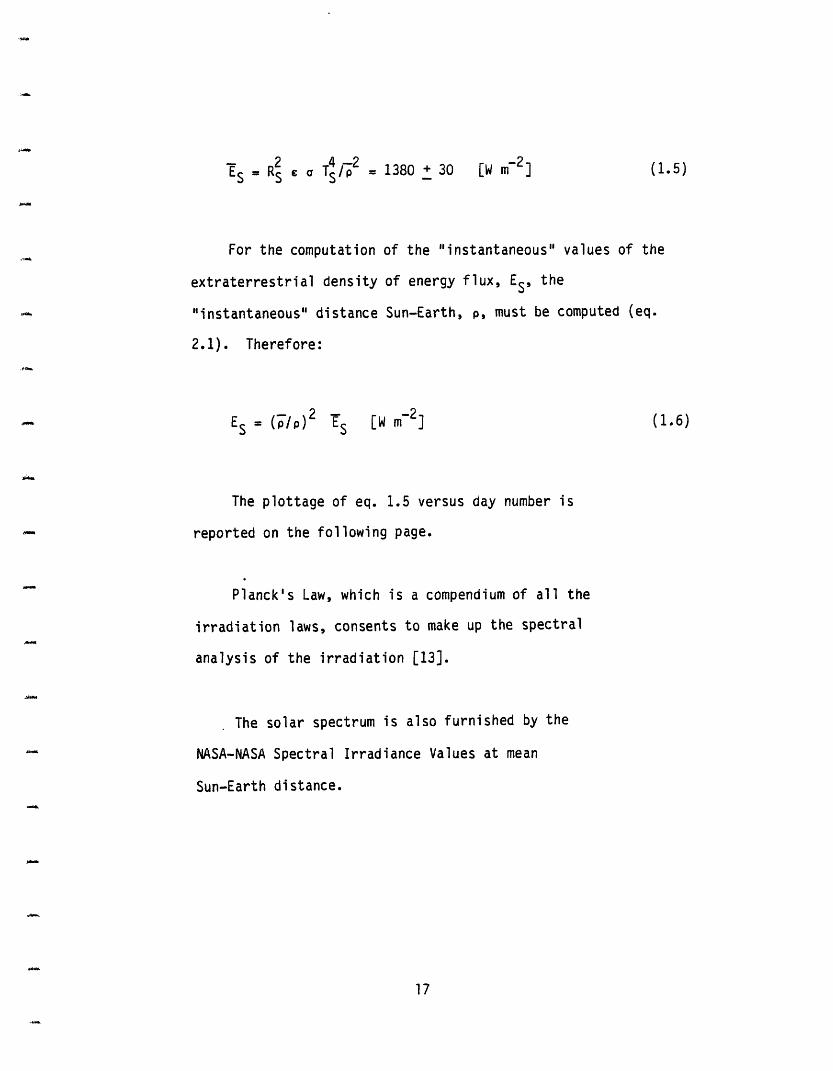
ES = RS E a T/2 = 1380 + 30 [W m 2] (1.5)
For the computation of the "instantaneous" values of the
extraterrestrial density of energy flux, E, the
"instantaneous" distance Sun-Earth, p, must be computed (eq.
2.1). Therefore:
ES = (T/P)2 Es [W m 2] (1.6)
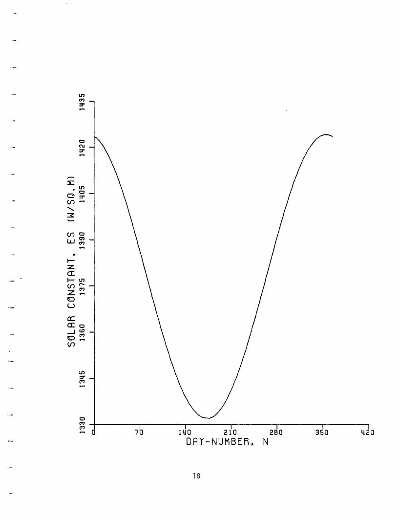
The plottage of eq. 1.5 versus day number is
reported on the following page.
Planck's Law, which is a compendium of all the
irradiation laws, consents to make up the spectral
analysis of the irradiation [13].
The solar spectrum is also furnished by the
NASA-NASA Spectral Irradiance Values at mean
Sun-Earth distance.
17
DRY-NUMBER, N
18
L,en
;3;
CU=6
ru
U,
(n
(f)0
(n 00,LJJcr,
1-,
(f)r -C,,
J0
Cr)Z cl
CD,
Cv,C,
0
CHAPTER 2
ASTRONOMICAL PARAMETERS
2.1 SUN-EARTH DISTANCE
This section considers the ideal case of a pure Sun-Earth
Newtonian system.
The parameters of the Earth orbit are known. From the
equation of the ellipse in polar coordinates, it is possible to
derive, through a trivial computation, the instantaneous
distance between the Sun and the Earth, , as a function of the
anomaly i (see Figures 1 and 2):
p = p/[1 + e cos(E)] (2.1)
= (N + 10) 2 r/365 (2.2)
where:
N = progressive number of the days of the year, first of
January, N = 1.
19
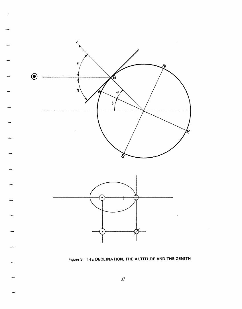
2.2 DECLINATION ANGLE
The rotation axis of the Earth is inclined with respect to
the normal to the plane of the ecliptic, at an angle = 230 27'.
This angle varies, owing to the precession motion; the
period of such motion is 25,800 years. The correspondent
variation of is only a few seconds a year, and may be
neglected.
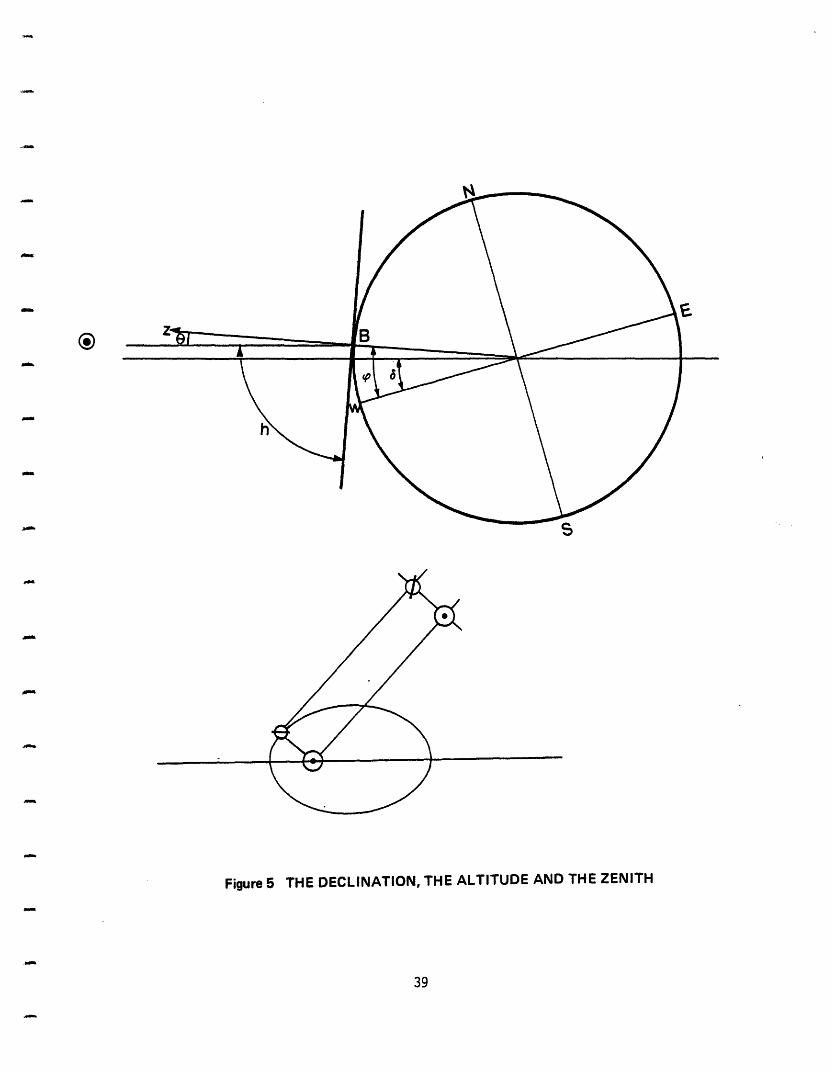
The declination, a, is defined as the angle between the
line connecting the center of the Earth to the center of the Sun
and the equatorial plane, i.e., the angle that the solar beam
forms with the equatorial plane (see Figures 3, 4, and 5).
The declination takes into account the dependence of the
inclination of the energy beam upon the Earth's position in its
orbit, even being a constant.
The inclination influences, ceteris paribus, the total
irradiance on the ground and is the cause of the Earth's
seasonal cycles. At the summer and winter solstices, s equals
+C and - respectively; at the equinoxes, s equals zero and
the length of day equals the length of night, thus:
20
-23° 27' < < + 230 27'.
The value of may be derived within an approximation of
20' - 30', from the following expression:
6 = 23' 27' cos[180(A + N + T/24)/186]' [deg] (2.3)
where:
A = 13 (12 on leap years) [adimensional]
T = G.M.T. (Greenwich Mean Time) [hours].
The declination varies from 0 to every 365/4 days: a
variation of about 15' a day. In the calculations we will
assume a daily average value for a, called 60, obtained from eq.
2.3 for T = 12.
2.3 AZIMUTH AND ALTITUDE OF THE SUN
The instantaneous position of the Sun with respect to a
frame solidary with the Earth determines the trajectory of the
apparent motion of the Sun.
21
We will determine the general law that relates the
altitude, h, and the azimuth, , of the Sun to the latitude, +,
the longitude, , and the period of the year, as a function of
time.
The latitude and the longitude of point B, where the
observer stands, are known.
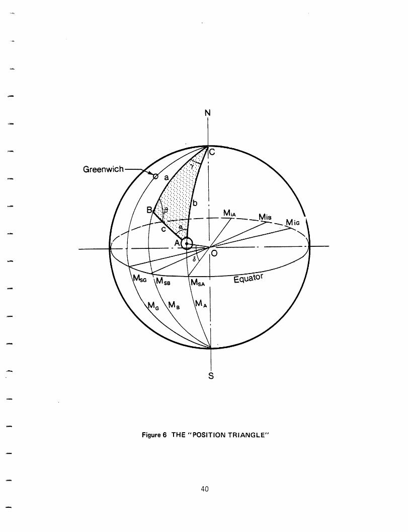
Using the Eulero formulas, we solve the spherical triangle
ABC ("position triangle"), where A is the subastral point of the
Sun, B is the observer's position, and C is the extreme pole of
the observer's hemisphere (see Figure 6):
BOC a = 90 -- (2.4)
AOC = b = 90 - a (2.5)
AOB = c = 900 - h (2.6)
cos(a) = cos(b) cos(c) + sin(b) sin(c) cos(a) (2.7)
cos(b) = cos(c) cos(a) + sin(c) sin(a) cos(s) (2.8)
cos(c) = cos(a) cos(b) + sin(a) sin(b) cos(y) (2.9)
2.3.1 Altitude
From eqs. 2.4, 2.5, 2.6, and 2.9 we derive the following
equation:
22
sin(h) = sin(^) sin(q) + cos(s) cos(4) cos(y)
The pole angle, y, of the position triangle varies with
time, because the subastral point of the Sun, A, shifts during
the day due to rotation.*
Conventionally, solar time, t, is zero when the subastral
point of the Sun is on the antimeridian of the observer. Then:
y = 180 - t = 180 - (T + x) (2.11)
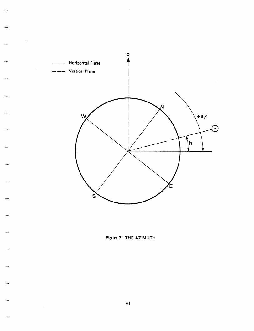
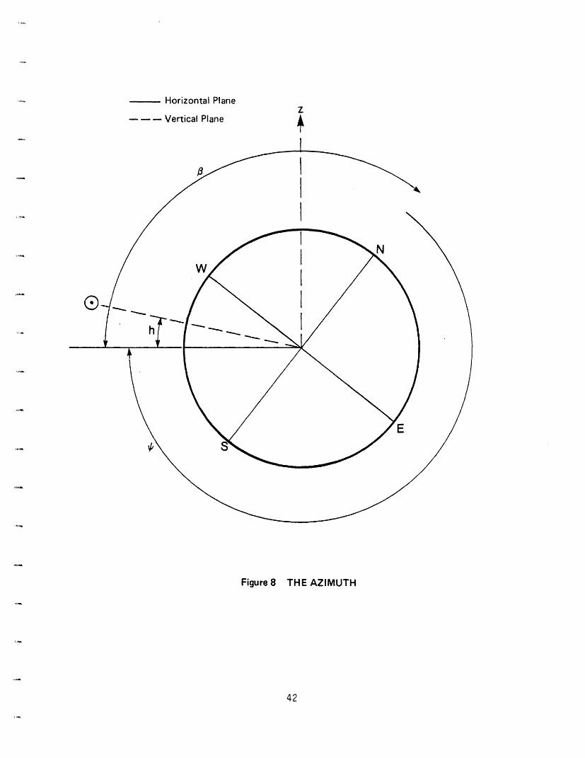
2.3.2 Azimuth
The azimuth, A, is the angle between the projection on the
horizontal plane (plane of the observer) of the meridian and
the (instantaneous) Sun-Earth axis. Conventionally, the
azimuth is measured clockwise from the North, from 0 to 360
degrees. Thus, the azimuth is equal to the angle for p
between 0 and 180 degrees (see Figure 7) and is equal to the
complement to 360 degrees of for between 180 and 360
degrees (see Figure 8):
*One complete rotation of the Earth takes 24 hours; onehour corresponds to 360/24 degrees. From now on, angles willbe given either in degrees or in hours, assuming implicitconversion when necessary.
23
(2.10)
= EAST
= 360° - 8wEST (2.13)
The angle varies between 0
5), East in antimeridian and West
general expression of (eqs. 2.4,
and 180 degrees (see Figure
in postmeridian hours; the
2.5, 2.6, 2.8) is:
cos(s) = [sin(s) - sin(h) sin(f)]/[cos(h) cos(f)] (2.14)
2.4 DAYTIME
We assume that the daytime period, D, is equal to the time
between geometrical sunrise and sunset.
However, the daytime period is actually higher than the
time we assume as D, since the Earth "sees" the Sun under an
angle of about 30', and atmospheric refraction brings solar
radiation to the ground when the Sun is one degree below the
horizon.
From eq. 2.10, recalling that at the instant of sunrise h
equals zero and calling y' the angle at that instant, we
24
(2.12)
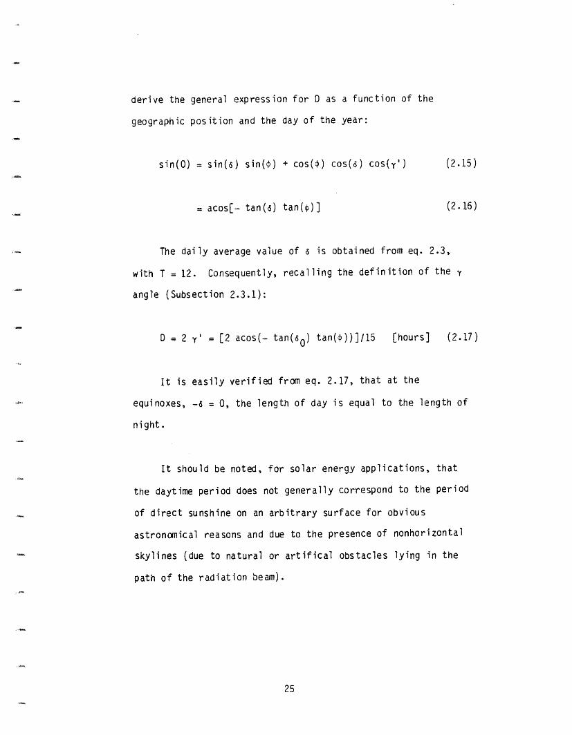
derive the general expression for D as a function of the
geographic position and the day of the year:
sin(O) = sin(6) sin(f) + cos(4) cos(s) cos(y')
= acos[- tan(s) tan(+)]
(2.15)
(2.16)
The daily average value of is obtained from eq. 2.3,
with T = 12. Consequently, recalling the definition of the y
angle (Subsection 2.3.1):
D=2
It is
equinoxes,
night.
y' = [2 acos(- tan(60) tan(f))]/15 [hours] (2.17)
easily verified from eq. 2.17, that at the
-s O0, the length of day is equal to the length of
It should be noted, for solar energy applications, that
the daytime period does not generally correspond to the period
of direct sunshine on an arbitrary surface for obvious
astronomical reasons and due to the presence of nonhorizontal
skylines (due to natural or artifical obstacles lying in the
path of the radiation beam).
25
This paper will develop one way to compute such an
"apparent" daytime on a surface for some typical cases,
although the easier computation would be an implicit one, upon
implementation of this model [14,15].
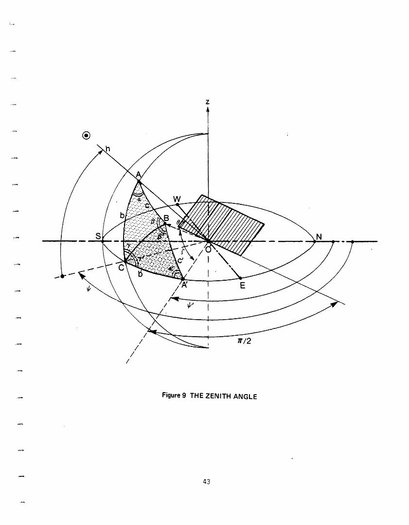
2.5 ZENITH ANGLE
The angle formed between the Sun's ray and the normal to
the surface under consideration is called the zenith angle, e
(see Figure 9).
The inclination angle of the slant surface, , will be
defined as the angle formed between the normal to the surface
and the horizontal plane (see Figure 9).
The orientation angle of the slant surface, ', will be
defined as the angle formed between the projection on the
horizontal plane of the normal to the surface and the superior
pole. This angle can be visualized if it is thought of as the
"azimuth" angle of the normal to the surface (see Figure 9).
It should be noted that, for the complete individuation of
a slant surface, two angles are needed. The definition and the
choice of the inclination and the orientation given above,
26
however, are arbitrary and do not correspond to any
"normalized" (and nonexistent) notation.
Using Eulero's formulas to solve the spheric triangles ABC
and A'BC and using the spheric rectangular triangle formulas to
solve the rectangular spheric triangles OAB, OA'B, and OBC (see
Figure 9), an expression of the zenith angle as a function of
Sun's altitude, azimuth, and the inclination and the
orientation of the slant surface, is easily obtained:
cos(e) = cos(i - 'I) cos(C) cos(h) + [1 + cos (j - 'I) cos (c)]1/2
sin(h) sin(y') ( 2.18)
where:
y' = atan[tan(c)/sin(j - '1J)]. (2.19)
2.6 EXAMPLES
This section performs a few computations with the formulas
previously defined; they should be considered examples and will
provide an idea of the order of magnitude of the computation
error.
27
2.6.1 Declination angle computation
Derive the declination of 15 h 00 m G.M.T. on April 18th
of a "common year."
The input data are:
T = 15.00 hours, N = 108, A = 13.
Therefore, using eq. 2.3:
6 = -230 27' cos[.9677(108 + 13 + 15/24)]1 = 10.90 degrees = 10° 54'
For a leap year, same day and time, the result would not
change because the input data would be T = 15, N = 109, and A =
12. The total between parentheses would be the same.
The ephemerides values of the declination,
time considered, are:
1970 ("common year"):
1972 ("leap year"):
for the day and
6 = + 10 49'
6 = + 11° 00'
It should be pointed out that the error changes with the
date, but largely within the limits of accuracy.
28
2.6.2 Solar altitude computation
Derive the solar altitude at Nome, Alaska (lat.: 640 30'
N; long.: 165 ° 24' W) at 10 h 22 m on February 26th, 1972.
The input data are:
= 64° 30' N, x = 1650 24' W, t = 10 h 22 m, N = 57,
A = 12
The longitude value shows that Nome is eleven hours West
of Greenwich (the eleventh time zone West going from x = 1570
30' to x = 172 ° 30'). Therefore, the correspondent G.M.T. may
be computed:
local time + 11 h 00 m = G.M.T.
10 h 22 m + 11 h 00 m = 21 h 22 m G.M.T.
Conversion of G.M.T. into degrees:
(21 h 00 m + 22/60)15 = 320.50 degrees = 320' 30'
The y angle is computed from eq. 2.11:
-= 180 - (3200 30' - 1659 24') = + 24° 54'
29
Proceeding as indicated by Subsection 2.5.1, the
declination is computed:
6 = - 8 55'
The exact value of the declination, from the ephemerides,
is - 8 48'.
The solar altitude, h, is computed from eq. 2.10:
h = asin[sin(- 8 55') sin(64 ° 30') + cos(- 8° 55')
cos(64' 30') cos(24" 54')] = 14.23 degrees
= 14' 14'
or, with the exact value of the declination:
h = asin[sin(- 8 48') sin(64" 30') + cos(- 8 48')
cos(64 ° 30') cos(24° 54')] = 14.34 degrees
= 140 20'
2.6.3 Solar Azimuth Computation
Derive the solar azimuth at Nome, Alaska (lat: 64' 30' N;
long.: 165 ° 24' W) at 10 h 22 m on February 26th, 1972.
30
The input data are:
= 640 30' N, = 1650 24' W, t = 10 h 22 m
and, from Subsections 2.5.1 and 2.5.2:
a = - 80 55' (exact value: - 8° 48')
h = 14 14' (exact value: 14' 20')
From eq. 2.14 the angle of the "position triangle" is
computed:
sin(- 8° 55') - sin(l4 14') sin(64 30')]acos[ cos(l4' 14') cos(64 30')
= 154.59 degrees East = 1540 35' E
or, with the exact values of a and h:
acosin(- 8 48') - sin(14' 20') sin(64" 30')]acB = acos(14- 20') cos(64- 30')
= 154.48 degrees East = 1540 29' E
Thus, from eq. 2.12:
= 154' 35' (exact value: 1540 29')
31
2.6.4 Geometrical Daylength Computation
Compute the length of the day at Nome, Alaska (lat: 640
30' N; long.: 1650 24' w) for April 18th, 1970:
Since the precession motion is not being considered, the
year datum will not be used as input. The longitude will not
affect the daylength.
The input data are:
+ = 64° 30' N, N = 108, A = 13
From Subsection 2.6.1:
60 = - 23° 27' cos[.9677(108 + 13 + 12 = 10.85 degrees
= 10° 51'
From eq. 2.17:
D = [2 acos(- tan(10 ° 51')) tan(64 ° 30')]/15
= 15.16 hours = 15 h 10 m
32
or, with the exact value of the declination:
D = [2 acos(- tan(10 ° 49'))tan(64 0 30')]/15
= 15.15 hours = 15 h 09 m
2.6.5 Problems
Further examples might be:
1. Computation of the meridian altitude of the Sun (i.e.,
maximum daily altitude of the Sun for a given location):
hmax = 90 - ( + 6)
2. Meridian altitude at the tropics for solstices and
equinoxes,
3. Pole angle, y, value at noon,
4. Geometrical sunrise and sunset azimuth angles, for a
given location on a given day,
5. Declination angle value at the equinoxes (as a
function of latitude),
33
6. Declination angle value at the solstices,
7. Geometrical day length at the Equator for solstices,
8. Geometrical day length at the Arctic Polar Circle for
solstices,
9. Geometrical day length for an equinox (is it possible,
without specifying the location?), and
10. Geometrical length of the polar night.
JM
34
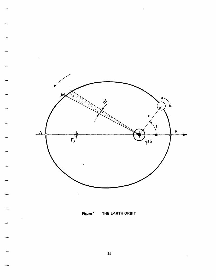
Figure 1 THE EARTH ORBIT
35
zl-�
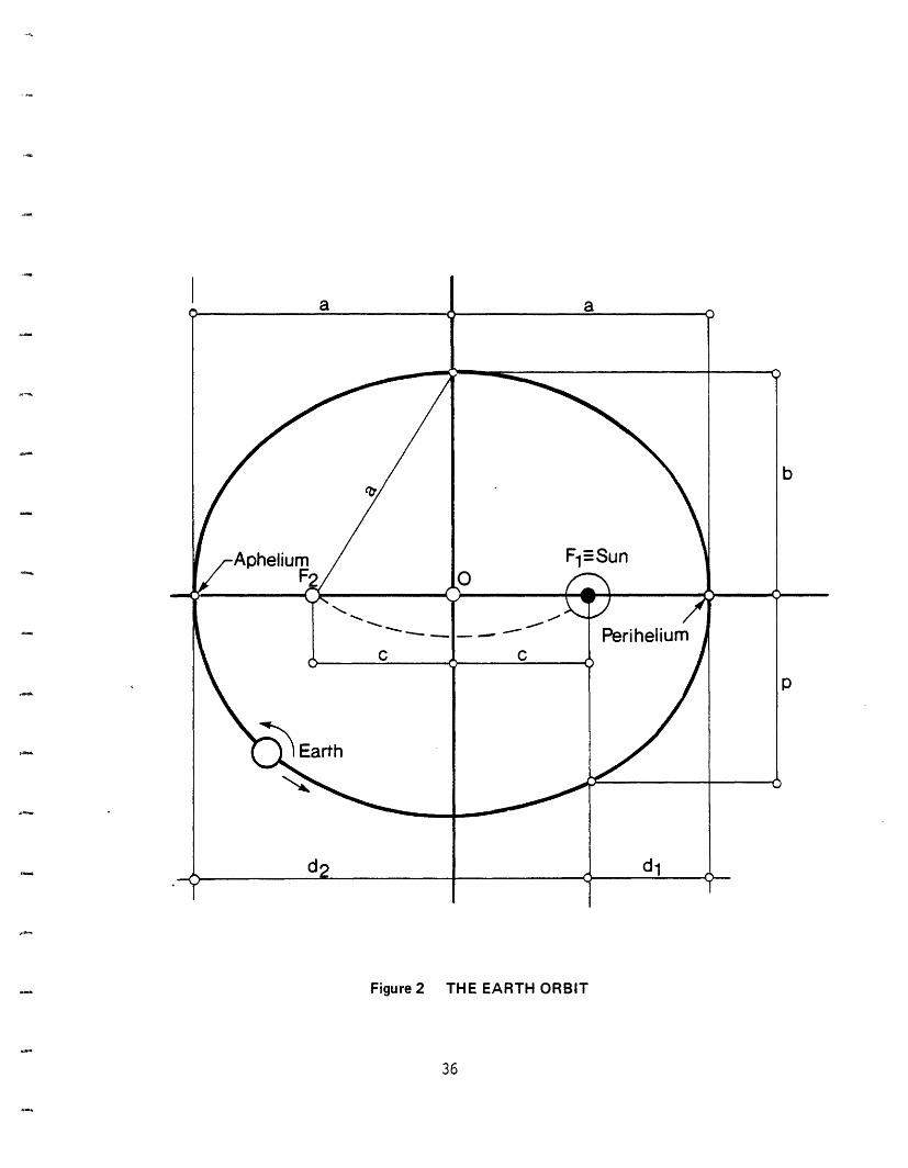
Figure 2 THE EARTH ORBIT
36
z
Figure 3 THE DECLINATION, THE ALTITUDE AND THE ZENITH
37
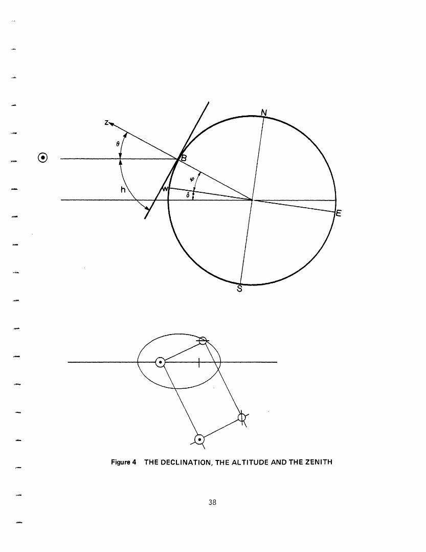
Figure 4 THE DECLINATION, THE ALTITUDE AND THE ZENITH
38
0-.
Figure 5 THE DECLINATION, THE ALTITUDE AND THE ZENITH
39
15
N
S
Figure 6 THE "POSITION TRIANGLE"
40
Horizontal Plane
Vertical Plane
Figure 7 THE AZIMUTH
41
Z
tIII
®0
Horizontal Plane
- - - Vertical Planei
Figure 8 THE AZIMUTH
42
z
N
71/2
Figure 9 THE ZENITH ANGLE
43
CHAPTER 3
INTERACTION OF THE SOLAR RADIATION WITH THE ATMOSPHERE
The interaction of the beam of radiative energy with
components of the atmosphere causes a depletion in the beam's
intensity and an alteration in the beam's characteristics, i.e.,
its spectrum and anisotropy.
The interaction is relative to the corpuscular and wave
characteristics of atmospheric components with respect to the
solar energy beam spectrum.
This interaction may be quantitatively analyzed in terms of
two phenomena: the radiation absorption and the radiation
scattering in the atmosphere. Both phenomena affect the
intensity and spectral composition of the radiation beam; the
latter will also substantially alter the beam characteristic of
the incident radiative energy.
44
3.1 RADIATION ABSORPTION IN THE ATMOSPHERE
The absorption spectrum of the atmosphere extends over an
extremely wide range, from X-ray to ultrashort waves. Thus, due
to the selective aspect of the interaction, the physical nature
of the absorption is highly varied and extremely complicated
[16,17].
One fundamental problem is determining the absorption
function--or its "complement," the transmission function-for
the entire solar spectral interval. It is useful to point out
that even under an integral approach, we cannot avoid
considering the spectral characteristics of the electromagnetic
radiation and its spectral interaction with the atmosphere.
In all cases, the main factor affecting the analysis will
be the atmospheric content of the radiation absorbent; however,
its behavior is not solely dependent on the spectrum of the
incident radiation or on its spectral lines but also in a number
of cases on the pressure and temperature of the radiation
absorbent.
Theoretically, when knowing the several principles of
spectral radiation absorption, the energy distribution of the
solar spectrum "outside" the atmosphere, and the dynamic
45
behavior of the atmosphere, it is possible to develop an
analytical model of the interaction and, consequently, the
energy distribution of the solar spectrum on the Earth, after
absorption interaction.
Physically, the definition of the absorption function may
be obtained considering only the very fine structure of the
absorption spectrum. This is an extremely complicated approach,
due to the complexity of the spectrum considered, and even the
lines-and-bands model approach is far more precise with respect
to the meteorological data available [18-23].
On the other hand, the many empirical relations that
furnish the transmittance function of the atmosphere [24] are
obtained through largely macroclimatic approaches and the
approximations made on the model may exceed the uncertainty and
lack of meteorological data. This is probably why existing
analytical models of the atmosphere are either extremely
complicated, inconsistent with available data, or only empirical
approximations.
In order to develop a proper approach for our purposes, let
us first briefly and qualitatively examine the characteristics
of the absorption spectrum of the various components of the
atmosphere. A number of tabulations of the atmospheric
46
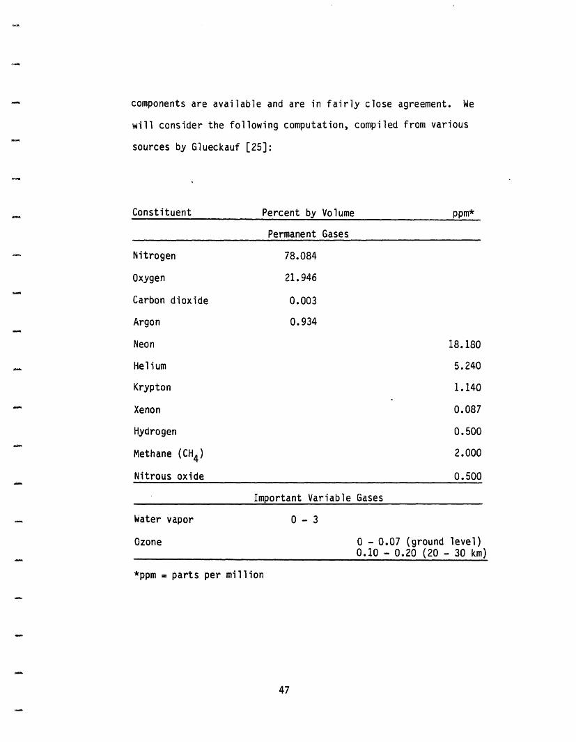
components are available and are in fairly close agreement. We
will consider the following computation, compiled from various
sources by Glueckauf [25]:
Constituent
Nitrogen
Oxygen
Carbon dioxide
Argon
Neon
Helium
Krypton
Xenon
Hydrogen
Methane (CH4)
Nitrous oxide
Percent by Volume
Permanent Gases
78.084
21.946
0.003
0.934
Important Variable Gases
Water vapor 0 - 3
Ozone 0 - 0.07 (ground level)0.10 - 0.20 (20 - 30 km)
*ppm parts per million
47
ppm*
18.180
5.240
1.140
0.087
0.500
2.000
0.500
-
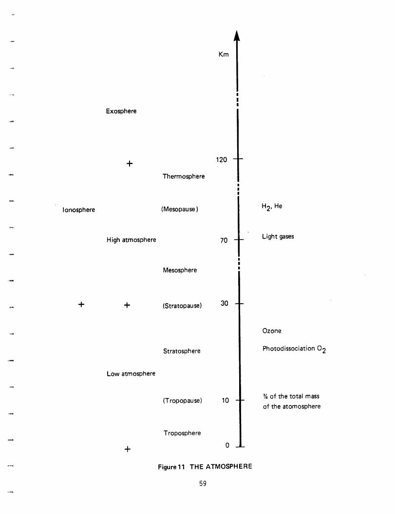
Finally, we will consider the atmosphere divided into
regions, as shown in Figure 11, using the altitude as an
extensive parameter.
Let us finally point out that three quarters of the total
mass of the atmosphere is in the troposphere.
3.1.1 The absorption spectrum of water vapor and water
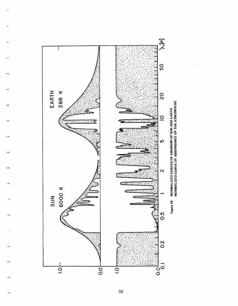
The atmospheric absorption spectrum is schematically
presented in Figure 10 [26]: The most intensive absorption
bands of the atmospheric gases are clearly individuated.
The main gases of the atmosphere, such as nitrogen and
oxygen, contribute only slightly to the radiation absorption.
The variable atmospheric constituents, such as water vapor,
oxygen and ozone (for the shortwave radiation), and carbon
dioxide, nitrogen, oxides, and hydrocarbon combinations (mainly
for the thermal radiation) have a number of absorption bands
(and lines) in various spectral regions.
As concerns solar radiation, the most intense absorption
bands are related to water vapor and ozone in the ultraviolet
48
region of the spectrum. The predominance of the water vapor in
atmospheric absorption caused by vibrational-rotational
transitions, is existent--and is a well-known effect--also due
to the fact that the energy content of the solar spectrum to
the frequencies affected by the ozone, is quite low.
The longwave radiation absorption, because it is affecting
the re-emitted radiation interaction, although we have
mentioned it, is not of interest and will not be discussed
further.
Moller [27] has proposed an empirical formula for the
calculation of the radiation absorption in the cloudless
atmosphere:
Rad. Abs. = exp[2.3026(- .740 - .347 log(m we))
- .056(log(m w)2 - .006(log(m w ))3)]
[cal cm-2 min-i]
where:
m = atmospheric mass
w, = total water vapor content in the atmosphere
in the vertical direction [g cm-2].
49
In order to account for the influence of pressure on the
radiation absorption, Moller proposed to use a value of the
pressure equal to 7/9 of the pressure of zero altitude.
Angstrom [28] proposed another formula that also takes
into account the scattering of solar radiation:
Rad. Abs. = .10[.23 w/(.23 w + )]
.21[1 - exp(- m ) exp(-.23 m )]
[cal cm-2 min-1]
where:
B = optical atmospheric mass caused by scattering.
Both these empirical relations and others available in the
literature are in fairly bad agreement. After analyzing the
available experimental data, it appears that a statistical
approach is the best for the absorption band model.
The water exerts its influence mainly on the thermal
radiation region, although water vapor has some nonintense
bands on the visible region of the spectrum.
50
3.1.2 The absorption spectrum of ozone and oxygen
Ozone has several absorption bands in the ultraviolet and
far-ultraviolet regions.
The computation of the integral of the solar radiation
flux absorbed by the ozone shows that the effect of the ozone
on the solar spectrum is extremely reduced (1 - 3 percent)
[29].
As concerns the oxygen, there are two visible bands in the
visible region, centered at .69 and .75 microns. Two other
bands, the Schumann-Runge system and the Herzberg system, are
located near the 2-micron region. Their influence on solar
radiation absorption is not great. The 1-micron
region--Holefield bands--is characterized by the presence of
unidentified, nonintensive bands. The main interest in the
study and analysis of these bands would be to individualize the
bands responsible for the dissociation-ozone "source" bands.
Atomic oxygen intensively absorbs radiation, but only in
the far-ultraviolet.
51
3.1.3 The absorption spectrum of minor radiation-absorbing
atmospheric constituents
There are nitrogen oxides (NO, N20, N204, ...,),
hydrocarbon combinations (CH4, C2H4, C2H6, ...), sulfurous
gases, heavy water (H30) and other very minor
radiation-absorbing components. Their weak and very narrow
absorption bands are located mainly in the infrared spectrum,
from 3 to 5 microns [30].
As a conclusion we might state that in the case of
shortwave radiation the absorption by water vapor strongly
predominates, while in the case of longwave radiation (thermal
radiation) carbon dioxide also plays an important role.
We will therefore consider water vapor as the only
variable component of the atmosphere, at least under a
macroclimatic approach, when calculating the transmission
function. Although water vapor usually comprises less than 3
percent of atmospheric gases, even under the particularly moist
conditions found at sea level, it may absorb up to five times
as much solar radiative energy as do all the other gases
combined. Although we are not interested in the phenomenon,
water vapor's role is predominant also as concerns the gaseous
absorption of the terrestrial radiation. A simple explanation
52
of this may be given by analyzing the vibrational and
rotational motions induced on the water molecules.
To compute the integral absorption function, two different
methods are generally used: the "spectral" method (by Elsevier
and by Kondratyev), which uses the spectral absorption
characteristics, and the "integral" method (by Brooks and by
Robinson), which uses integral absorption data.
3.2 RADIATION SCATTERING IN THE ATMOSPHERE
As has already been pointed out, the scattering of the
radiation is the second main process that characterizes the
interaction between the radiation beam and the components of
the atmosphere, as concerns the solar radiation. For the
longwave radiation, the medium's emission should also be taken
into account.
The so-called diffuse component of the solar radiation
beam on the Earth is the amount of scattered radiation that
arrives on the Earth.
Scattering phenomena are present in any location where
there is a spatial inhomogeneity of the dielectric constant of
53
the medium in which the radiation is traveling. These spatial
inhomogeneities that determine scattering may be caused by
fluctuations of a physical parameter that individuates the
state of the medium (e.g., air density) and by the localized
presence of particular components (e.g., water droplets, dust
particles, haze, smoke, etc.).
The first type of scattering is known as molecular
scattering. This definition is clearly understood if we take
into consideration that in this case the refraction index
inhomogeneities are of the same order of magnitude as the
conventional "physical" dimensions of molecules.
If the dimensions of the scattering particles are sensibly
smaller than the wavelength of the incident radiation (e.g., if
the dimensions of the scattering medium are sensibly smaller
than the wavelength), then the scattering is Rayleigh
scattering (or molecular scattering of Rayleigh).
The scattering caused by water droplets or other "large"
components is known as aerosol scattering, or as dry aerosol in
the case of dust particles.
Let us consider, in a chemical approach, a scattering
medium and a radiation beam traveling within it. For each
54
wavelength, the infinitesimal amount of radiant energy dE(x, )
scattered by the components present in an infinitesimal volume
dr on an infinitesimal solid angle d on the direction of --t
being the angle between the scattered ray considered and the
incident beam-will be:
dEs(x, P) = a(x, ) E(x) dr d (3.1)
where E(x) is the monochromatic density of energy flux of the
incident beam and (x, ) is a volume coefficient of radiation
scattering, for the wavelength and angle of scatter
considered. The a factor will also depend upon the optical
properties of the scattering medium. We express a as:
a(X, f) = (X) (p) (3.2)
where ~(q) is the scattering function that defines the
intensity of the scattered ray at an angle , and p(x) is the
parameter that takes into account the optical properties of the
scattering medium.
To compute the density of energy flux scattered over a
solid angle, by dr, eq. 3.1 may be rewritten (following eq. 3.2)
as:
55
ES(X) = 2 p(X) E(x) dr ( ( sin(Q) d (3.3)0
Normalizing dr, the volume scattering coefficient, (X)
may be defined as:
ES(~)(X) = = 2 ( (X,) (f) sin(f) d (3.4)
The theory of electromagnetic scattering would consent the
evaluation of the parameter p(X) and the function (f). Under
an empirical approach, the elaboration of the experimental data
available would furnish approximated values of the (x, P)
[31-33].
The electromagnetic scattering theory, although very
accurate under nonlimitative assumptions in describing
molecular and aerosol scattering, requires a complete
definition of the scattering medium. This complete definition,
particularly for local or aleatory aerosol conditions, is very
difficult to obtain.
Once again, empirical relations that are largely
macroclimatic are not of interest here. Instead, the widely
used semi-empirical approach of Angstrom [34] will be quoted.
56
This approach uses a so-called turbidity factor, which may be
computed rather precisely from direct irradiance data.
57
0 0
0
0w
Caw
oULO : v
- 0DI-cn
0<
ou-uJ
0 UW W
N N
00
.) U.
CVN
OUa
58
Km
Exosphere
120+
Thermosphere
(Mesopause)
High atmosphere 70
IMesosphere
+ (Stratopause) 30
Stratosphere
Low atmosphere
(Tropopause) 10
Troposphere
0
H2 , He
Light gases
Ozone
Photodissociation 02
3 of the total mass
of the atomosphere
Figure 11 THE ATMOSPHERE
59
II
Ionosphere
+
+
1 L
-
-
CHAPTER 4
SOLAR ENERGY RADIATIVE FLUX DEPLETION
Chapter 3 performed a general analysis of the interaction
of the radiative energy beam with the components of the
atmosphere.
This chapter will derive a physical model to describe the
solar energy radiative flux depletion in its atmospheric path,
taking the input data constraints into consideration.
A simple physical consideration of the interaction of the
radiation beam with the atmosphere, accepting the nonlimitative
assumption that the gas molecules do not "shadow" each other,
will permit the evaluation of the attenuation of a flux of
direct radiation, i.e., solar beam, through a slab, dz, of
atmosphere of density p(z) for each wavelength x:*
*Equation 4.1 might be rewritten as follows: dE(x)/dz =
K(x) E(x) p(z), which is the analytical representation of thefact that the attenuation of the beam on an arbitrary path dz inthe atmosphere is linearly propotional, for every wavelength, tothe number of nuclei per unit volume and to the intensity of theincident beam through a parameter of proptionality, here definedas K(x). Since the beam's depletion is linearly proportional todz through a parameter which is a function of x only, the beam'sTe'pletion with respect to z will be, as expected, exponential.
60
dE(x) = E(x) K(x) (z) dz
where K(x) is the absorbance "constant" for a determined gas
and wavelength , and z is the altitude of the slab dz
considered.
Integration, between elevation zero and elevation Z of eq.
4.1, gives:
EZ () j ZIn E(X ) =- K(x) 0EO~~~x Z
p(z) dz (4.2)
or:
ZEO(X) = EZ(x) exp[- K(x) f p(z) dz] (4.3)
where:
EZ(x) = density of energy flux of wavelength x at elevation
Z [W m-2]
Eo(x) = density of energy flux of wavelength x at elevation
o [w m-2].
Equation 4.3 is often called Beer's (or Bouguer's) Law.
61
(4.1)
The exponent of the exponential factor in the second term
of eq. 4.3 is often called "optical depth." Sometimes, the
integral term of the exponent is also referred to as "optical
depth," although it represents only a mass concept, being a
"density integral."
If the Sun is at the zenith, the beam's path will be on
the z axis (elevation or zenith axis), then an integration over
all the atmospheric path-let us say from 0 to --will furnish
the attenuation of the beam on its atmospheric path:
EO(x) = Ei(x) exp[- K(x) o(z) dz] (44)
where:
Ei(x) = density of energy flux incident on the "upper
limit" of the atmosphere [W m-2].
4.1 OPTICAL DEPTH FOR A VERTICAL PATH
Halley's Law gives the variation of atmospheric density
with the altitude, z; here it will be extended to the entire
atmosphere. This will permit computation of the integral
factor in eq. 4.4, a factor that will be defined as AO. As
stated in Halley's Law:
62
A(z=0) = A0 = J
where:
A(z=O) =
0(O) =
=
P(O) =
p(z) dz = O
p(O) exp[- z (O) g/P(O)] dz(4.5)
density integral of the atmosphere [kg m-2]
density of the atmosphere at z = 0 [kg m-3]
acceleration of gravity [m s-2]
atmospheric pressure at z = 0 [N m-2].
Developing the trivial integral
AO = p(O) [P(O)/(p(O) g)]
in eq. 4.5:
(4.6)
The term between parentheses is often referred to as
equivalent height (or scale height), H, of the atmosphere,
i.e., the height the atmosphere would have given that its
density is invariable with height and equal to p(O). Thus:
H = P(O)/(p(O) g)
Equation 4.5 may be rewritten as:
AO = p(O) H = P(O)/g
63
(4.7)
(4.8)
Obviously, if the optical depth of the atmosphere is
computed for a site at a certain altitude, its value will be
different from A0 K(x), since A depends on the elevation.
For an altitude zo, eq. 4.5 might be rewritten as:
A(z=z )= Az = z (z) dz z p(O) exp[- z p(O) g/P(O)] dz0 ~~~~~0 0 ~(4.9)
Developing the trivial integral in eq. 4.9:
Az = p(O) H exp(- z /H) (4.10)o
As expected, the optical depth value for a zero elevation
is the superior limit of the optical depth value.
The upper limit of integration (infinity) for the
atmospheric density integral, although mathematically correct,
might create some misunderstandings in its physical
interpretation.
Initially assuming the elevation-observer's location, as
always to be equal to 0, and computing A0 as a function of z,
from eq. 4.9 the following is obtained:
Ao(z) = p(O) exp[- z p(O) g/P(O)] dz [kg m2 ] (4.11)
64
or:
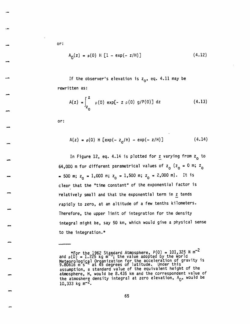
Ao(z) = p(O) H [1 - exp(- z/H)] (4.12)
If the observer's elevation is zo, eq. 4.11 may be
rewritten as:
zA(z) = p(O) exp[- z p(O) g/P(O)] dz (4.13)
or:
A(z) = p(O) H [exp(- zo/H) - exp(- z/H)] (4.14)
In Figure 12, eq. 4.14 is plotted for z varying from z to
64,000 m for different parametrical values of z (zo = 0 m; o
= 500 m; zo = 1,000 m; z = 1,500 m; zo = 2,000 m). It is
clear that the "time constant" of the exponential factor is
relatively small and that the exponential term in z tends
rapidly to zero, at an altitude of a few tenths kilometers.
Therefore, the upper limit of integration for the density
integral might be, say 50 km, which would give a physical sense
to the integration.*
*For the 1962 Sta~dard Atmosphere, P(O) = 101,325 N m-2and p(O) = 1.225 kg m- ; the value adopted by the WorldMeteorological Orqanization for the acceleration of gravity is9.80616 m s- at 45 degrees of latitude. Under thisassumption, a standard value of the equivalent height of theatmosphere, H, would be 8.435 km and the correspondent value ofthe atmoshere density integral at zero elevation, AO, would be10,333 kg m-2.
65
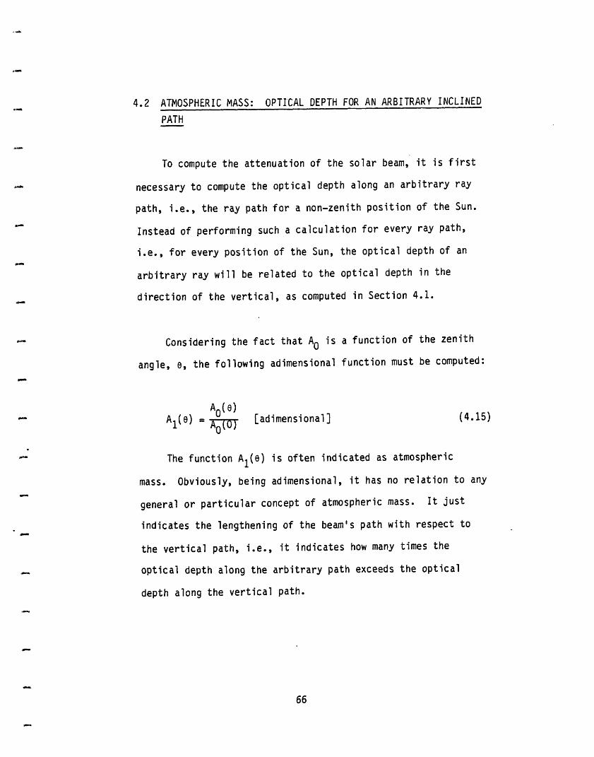
4.2 ATMOSPHERIC MASS: OPTICAL DEPTH FOR AN ARBITRARY INCLINED
PATH
To compute the attenuation of the solar beam, it is first
necessary to compute the optical depth along an arbitrary ray
path, i.e., the ray path for a non-zenith position of the Sun.
Instead of performing such a calculation for every ray path,
i.e., for every position of the Sun, the optical depth of an
arbitrary ray will be related to the optical depth in the
direction of the vertical, as computed in Section 4.1.
Considering the fact that A0 is a function of the zenith
angle, e, the following adimensional function must be computed:
Ao(e)Al (e) = o [adimensional] (4.15)
The function A1(e) is often indicated as atmospheric
mass. Obviously, being adimensional, it has no relation to any
general or particular concept of atmospheric mass. It just
indicates the lengthening of the beam's path with respect to
the vertical path, i.e., it indicates how many times the
optical depth along the arbitrary path exceeds the optical
depth along the vertical path.
66
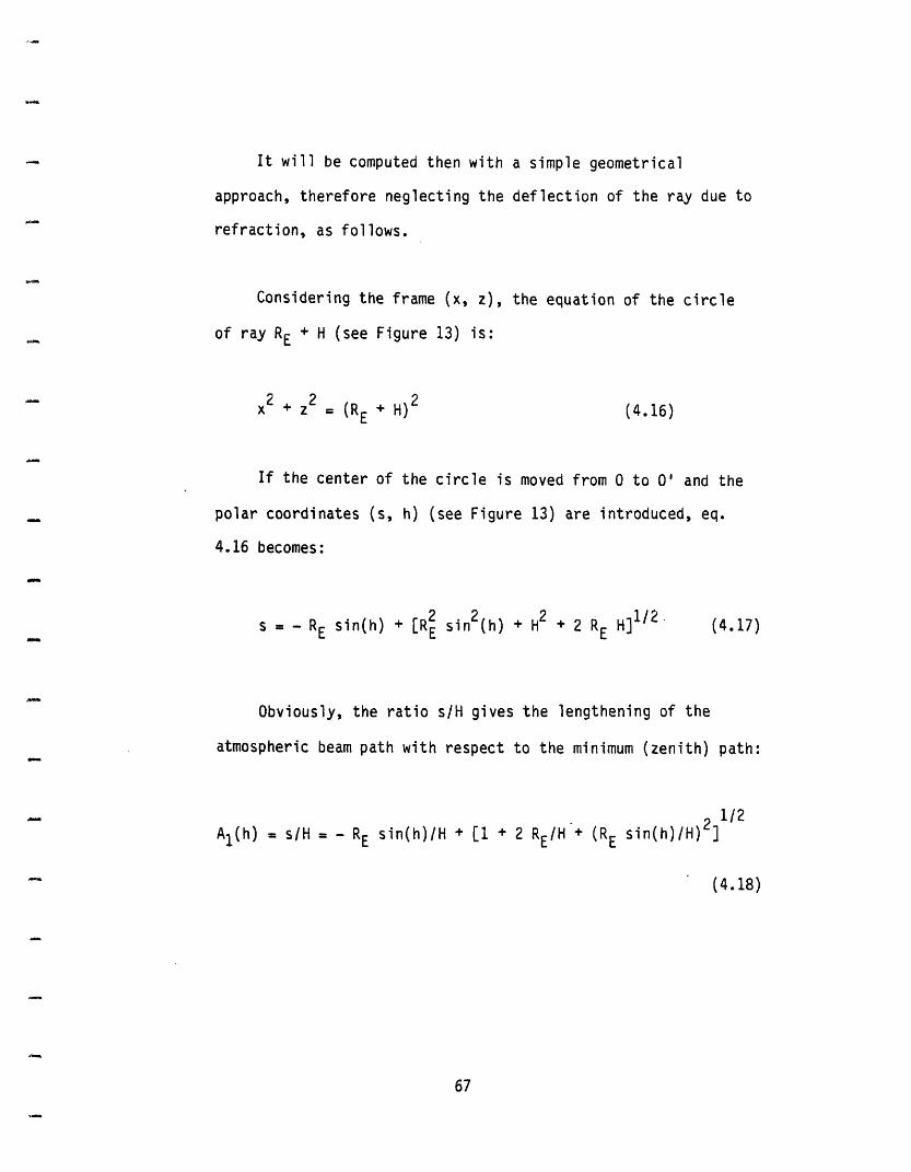
It will be computed then with a simple geometrical
approach, therefore neglecting the deflection of the ray due to
refraction, as follows.
Considering the frame (x, z), the equation of the circle
of ray RE + H (see Figure 13) is:
x2 + 2 = (RE + H) (4.16)
If the center of the circle is moved from 0 to 0' and the
polar coordinates (s, h) (see Figure 13) are introduced, eq.
4.16 becomes:
s = - RE sin(h) + [RE sin (h) + H2 + 2 RE H]1/2. (4.17)
Obviously, the ratio s/H gives the lengthening of the
atmospheric beam path with respect to the minimum (zenith) path:
1/2Al(h) = s/H = - RE sin(h)/H + [1 + 2 RE/H + (RE sin(h)/H) ]
(4.18)
67
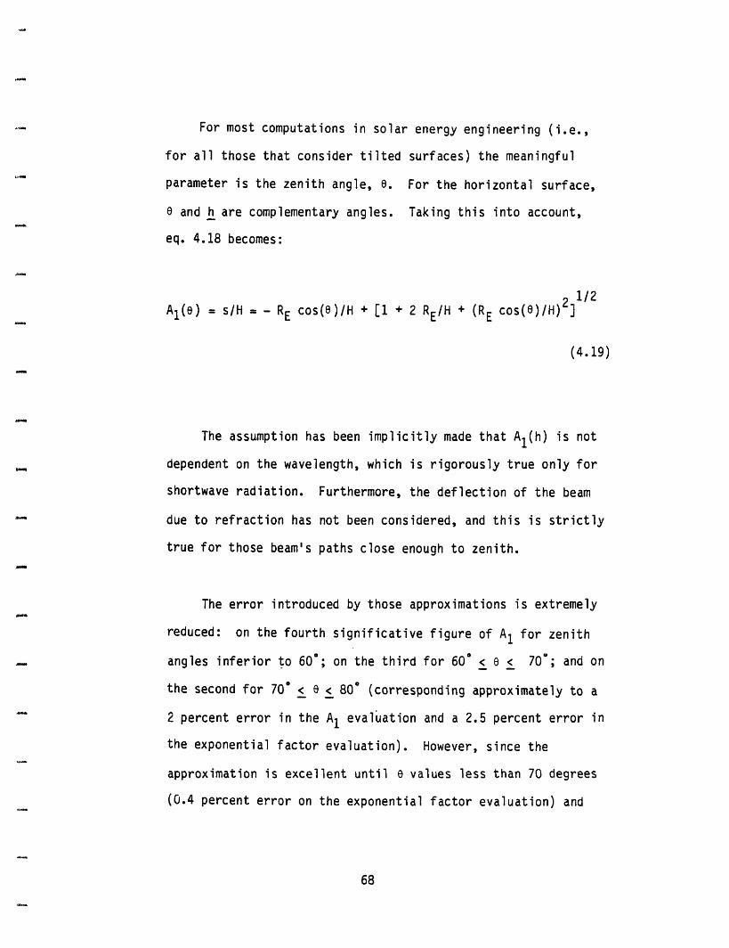
For most computations in solar energy engineering (i.e.,
for all those that consider tilted surfaces) the meaningful
parameter is the zenith angle, . For the horizontal surface,
e and h are complementary angles. Taking this into account,
eq. 4.18 becomes:
2 1/2Al(e) = s/H = - RE cos(e)/H + [1 + 2 RE/H + (RE cos(e)/H) ]
(4.19)
The assumption has been implicitly made that Al(h) is not
dependent on the wavelength, which is rigorously true only for
shortwave radiation. Furthermore, the deflection of the beam
due to refraction has not been considered, and this is strictly
true for those beam's paths close enough to zenith.
The error introduced by those approximations is extremely
reduced: on the fourth significative figure of A1 for zenith
angles inferior to 600; on the third for 60° < < 70°; and on
the second for 70 < e < 800 (corresponding approximately to a
2 percent error in the A evaluation and a 2.5 percent error in
the exponential factor evaluation). However, since the
approximation is excellent until e values less than 70 degrees
(0.4 percent error on the exponential factor evaluation) and
68
since for larger values of we are considering instants in
which the total amount of energy flux on the ground does not
exceed, in the extreme conditions (i.e., winter days), the 30
percent of the daily energy flux, then the maximum error
introduced in the transmission factor evaluation by the A1
computation is certainly not larger than 1.2 percent, and the
average error for the year is less than 0.5 percent.
Rewriting eq. 4.15 in an explicit form, the following
equation is obtained:
A1(O) = [J K(x) (s) ds]/[ K() p(z) dz] (4.20)
Equation 4.20 might suggest that A1(e) is strongly
dependent on atmospheric physical conditions (e.g., pressure
and temperature). But eq. 4.20 also shows that pressure
variations will not affect A(e) values, the density integrals
in numerator and denominator of eq. 4.20 being approximately
proportional to the physical mass of one atmospheric column of
unit section, which is itself proportional to the pressure at
sea level.
The temperature dependence is significant only at very
large zenith angles, where the density of energy flux of the
69
radiative beam is very low and the energy flux on the
horizontal of the observer is strongly affected by Lambert's
Law. It therefore may be neglected.
For quick computations of the atmospheric mass, mainly for
hand-pocket calculators, a simpler form of A(h) is often used:
A1(h) = sec(e) = cosec(h) (4.21)
For h values less than 30 degrees but greater than 10
degrees, the following empirical formula is often used:
A1(h) = (eq. 4.19) sec(e) - 2.8/(90 - )2 (4.22)= (eq. 4.17) cosec(h) - 2.8/h2
where e and h are expressed in degrees.
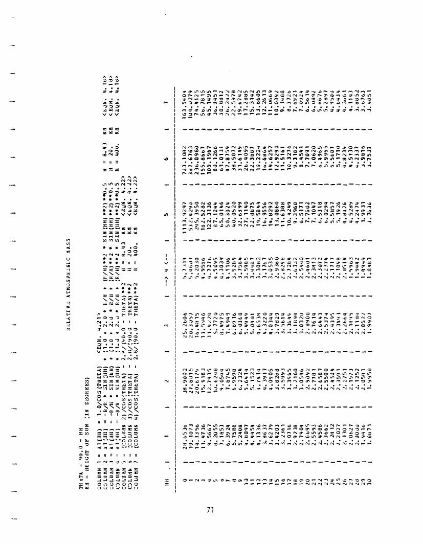
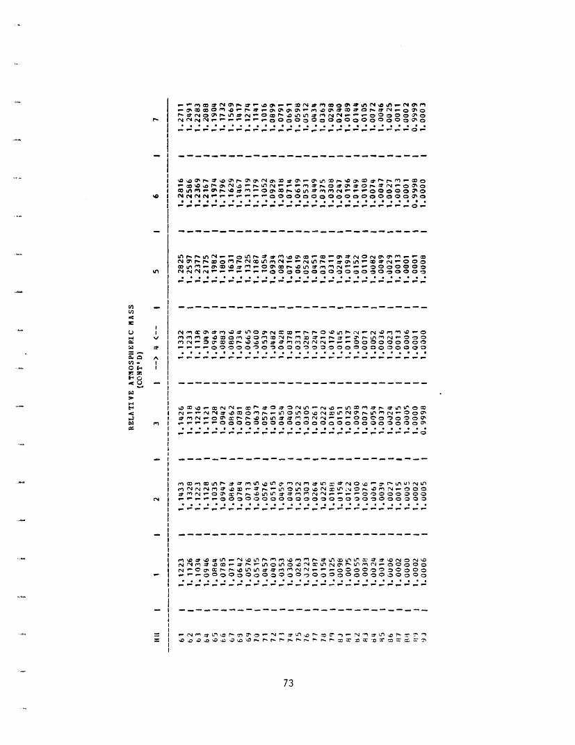
Equations 4.21, 4.18, and 4.22 are tabulated below; eqs.
4.18 and 4.22 in particular are computed for three different
values of H:
H = 8.4 km; H = 20 km; H = 400 km.
70
A A
V V Vvv v
I .u*o 0
ii Ii 11I
N
* * * *. "
N. N :. c-4* * * , -
* * * I VV
< -""" :Z ,.
* * * =
I I I I
2 00 0 I 0 o r Fu UU
-. . . . I I.Z X (93'
0- c- -r 0
v Ucnv _ :<: - =
P =s _- g - F ¢ - ZZ
E HH XX
_.,,^,(Znr
_- - 0 2
= -sa ssr24"30
_ _Y'D _- rJt}
'< #: < C ''@
_ .N > l 5°
Z Z ZZ ZZ
r + c r sC
a : an-nv
o= 3t * on
t.)tS J ) Qt
%0
Un
I
v
A
II
N
' os n n n U-4 N :0 N U N U ( 0 0 M o 3 N N.0 3 N- e - - -o N % n N I 3' 3 -V0 . 0 0 IN N tN 0% /7- 3' 0n 3' Wu 'o U,t N ". T _3' r M-It 0% - 0. 0 . 'la :1 0- t- n 0 0 ' 0 U ' 0 - z P' M
S - -t el. - 0 X 4ulO1 M .O " S-20 - 1 a S- )'D~ 1 : 1 -= Q-
,3 3' .r 0 U, . 0 .0 N 0 F- U, (9N -0 0 1- .0s0 U, * 3 : ' 93t _l ,\ oq t>$ _ _ _ _ _ _ _g
' rn (9 r. r l t- N M U` w 3' _ I 0" .° N' - 0 Ul I - 0 3% 0 .. O0 - o ' o o (9 ,n o 3 0% N tn , 0- = 3_ 3O N o % 0 - r O (n
-,,0 - . 0 M U'a N,0 0% IM O Pt * -0 -P 0 -W N M r.
4 9 a c,4-:9: :; 0~ * O 9 _ v. S rn t r,-
fN - 0 N - _(9~N".".NN~N~969N~
0 0 Nla _0 :? 0 0 0 U, 3 l aN 0 0 0- N - 3 t r 0 0% 3" .oo% %, 3 3' N N 0% 3' W'- 3' U, 0% %0 t 3 '0 0 3' 0 U, N N 0 W% t- ,tN N4 N n. re". 0 O (r - O N D (9 N 0% - Zo 0 "(N z 0% t ' N " 0 2VI * ( U, (9 0(90o *. U, 0% I0 00 o -It In rW- U 0 U, 0 U= N % el,
*4 * 'A * . * 'A * .3 . .z . .; * . * * . * . . . * .~ 'A . : * . 4 * In( VI M N 0 0t 3 (N N C .- O t '
-I Un "I _-UZ N _ _0t~0~r~9~9 ~
i 3- o ' 0 .r Ur ,j c, -3r O W- N r- o _ 00 3' ' NO " N 3' r- = 3'x m 3% (9n M - 0 ( G x a w0 .9 0% D I n S' 0" - r- 0- 3' ' ::t:
'0 - 0 U _ N 00 - N In 3 - U, m N 3' = 0 r- 0 U, : 3'| _ N 0% e- U ( 0 r L4 t.r? rV - O0 3% In - *U WI (9 M (9 C - - 3% " 0I~ ,; 4 ; ~; ; -4 . . .. * . . . . * . . . . . . * . S!, U,- L-l e 3' 3' 3' 3' (91 (9(9 (9(9( (9 Nf Ntte N N N N N s 'N N N NS- -
'0Q U, 0 3' U -U, _ w O 3 o :?0 *r 3' O 3' 0 0 3' (9 en U, (n 3 U, ' N I-0 U, - - N N °. 3' z 3' (n -* N 3'1 °N 0 3. a _% 3o 0 I 0,o 0 3 -N r 0% 3% a, (9 -. r s U N- z 00 Y = (95 -' ' .? ' -v (9 3 - U 0'4 ( 3' ul' 3' r- 3' * D 0 3' o .0(90 t, t " 0 a 1- a3 U, - - 0 -
U, 0 ,0( ". _' 0 C: t- '0U, U, 3' S' :r (9( (9(9(9 N N N No N 'N N 'N N N"1N N - - -
0 VI. 0 -1 (93' M 3' 3% S " "" 0 O : 3% t 0 4 N t 00% U - U, D,
0 "" W N UT .- _U, (9 _- U, 3' 3% ) N 0% ". U, 0% O z U U U', f r- N U V% = - - e r - u r0 0 M -N O (0 U, a- (9'n r - '0U, 3'n (9 rN ". N Lo G> 0 U, N 0 x .0 U, 3' 3 0 2 0 (9 a ( r- N N N N _ _" .
tN N " "" .S S 1 r4,N r* -
D3( l. 0 U, ( 3' 0 0 - r _ ' I rv 3 ( " ' 3 G , S' N - 1. 3 0 .0 ". I- U, M vD 9 .0 U, 4 U N 0 M 3 I U - O, 0 ( 0 3% 3% M 0 - C 0 N .- 1-U, 0 (9 r. , -W x '0 0 0% U, 3 a 0 3' (9. Na N (9 tl N M % .0 U, U0 0 (9.z 0 3'0 '3 ". 3 U, N " - (9 - N M 3'". 0 3 'N 0 a, . U, 7 r9en N N ".0 3n n -
.. S 0 9 * S _ 5 5N 0 % 3 ' 0 , U 9 9 9 N N N N ' N N N N N "~m~N".m ~ ~9'ON
0". N (9 ' U, 0 t. = Is ". - 34 " U . 0 D 0 = " - N 9 3 Un D - C -- - -- - - - -- ~4 N 4 S4 'J ~,N N4 rJ No I^ n
71
Entn
U0nuU,
c
0
H:nearZIs
-
U,
C;
zt-n
IAw0
j.i
I
0=
E=

0 ' 0Ln t M 0 N rN N N *4 L N M * p t- 0 LA N 0% L N *uo 0% * --no 0 N 'o o o000 '0 oA O N 00 " P * N M oa 0 a*-_ 0 a n1 N p.- N tn L g- 0 * X N_ '0N ° * 0'D o r0 _ - 0
_-- 0) o ul '0A N _- o % 0 0 1% b '.0 'e LA LA LA * t~ x e' NM * 0 M 0i a 0 r M N 0 0 S W w - - 5 n 0 z - -r * m *
enPIr N N N N N C4 N N N4C N p. -0 p. p. 0 . p. p. p. p. "
0% 00 as % N N 0 - x * LA 0 LA 0% 0% M. * 0 _ DO L L 0 * 0'00 f- r o M - M 0S :0 L 0 '0o M r 0 MzD _ M 0 7 c N z0* LA 0 N 0 t - - N -t ' 0% N'0o L 0 a 0 N MN 0 W'.o M 0
M - 0 r-5 0 0 - 0 5 w 0 t a 0 v 0 0 M M M
44,444N4N N NNNN NNNN N-'-.
rL 0 Mc N 0 M 0 0 la o ' *t N u * M N M r cM Ln o 0 0 %0-A w 0 N _ -Q 0 -t M .. 0n 0 a * S-% 0 M 0
LA '0 0% I' 0% L M N -' N t r r Q 0 LA 0 L 0 '0N M 0n LA 0 M , 0L M 9 0 r LA M N 0 0 O* o r - . 0 LA LA * _ - M M M en
* N N N . . . . . . . . * . . . . . . . . . . *. .xte^ N N NN4 NN _----- _- - - - - - _
N r? f" 0 M M N * 0% '0D Z r- M 0% M r M b Cy 0 : '0 *r 0% c. *W LA:r N N a, 0 LA M N M VI M e 0 '0 * M M : '00 N D-rv m 0 ! L r * 0 'O N 0 *- - LA N 0% '0 p- - e7 LA o - _% r- '0 r m o c Ln ur
o r r 'D uD o * 0 0 Un -r 5 M . M M M 4 0 N SN 0 0 _ _ _
o. p...- p . . . . . . p .. p~~. . - . . . . . . .__ _ __ _ __ _ __ _ _ ------ _.-- - -- - - - - -_: ~ O m~~~~~~~~~~~t
N 0o N 0' 0 N N *-3 - 0 0 0 * 0% 3 t00% t-- : * L -'90% 0% N f_ '0 1 0 N - p- M IN 0 1-M ' r'- *v '-0 MD M9 1t N M C 0 N L N '"a I '0 tN 0 z 0 r9 - 0% f 'LAON 0 w 1 p F.0 '0'0 L A t 3 3n (' e N N N N N '- - --
.****bN"g0.*.*.*. ... *..*..*.._ _ _ _ _ _ _ _ _ _ _p_ _ _. _. _ _ _ . .
0 0 0 ON N M 0' Q = N. 1N LI 1 * Ln N N * M '-0 e- 0 a f- V(M T LA l - 0% ;J N .. 3 N M A 0 1a 0% '0 * LA7 0 _ LA 0 LA - a 'M M ' o * 0 N M Lit N Cm O M -w 0. * 1 N = ' LA, -r N 0 - .0o 0 5 (% I.. a0 o %OLA V LA *-r * * * 'l "9 " ' 9n n N N N N N N0 _ p p p4 1* *_ . I. * **-I* 0 5 *0 S 0 * I
_____ _-____-____-__q_-____-_-
- -t M' a '0 0 eI n 'o N N n 0 a* x p. -. N :? N _ - * r^O * ' N a, LA N) 3% .1 a, ' * N 0 LAVNl 7 N OJ 0 0N .0 LA :r M N
0'0%0LALALA****(m('9NNNNNN.'-r'-p;M 0 .. 5a N M I 5 t 4 - C 4 1 4 0 - - 1co P- fl r- I4~ n t _- _- -T M fn M te rn r4 N N N rq- -- -- -I .@@@**** I .***.e
- N4 In1 L ' f 0- M 5 - N I = L o 0 - 0 N N - L -D f- = 0M M (' ( n ( " '9 * * * * * * * * * * LA o LA uL LA LA LA LI Ln L -
72
tn
r z
cm-ccu
EsOE-:0
z
-c 43
cr
!
V
I
I
=II
f
-'-Mml 0 2 NM P% -- " 9- 47 0% "M-0N& MM* MOa * N L - N %MM*% M M 0 m 9 - r- -0% % 0% % - M '0 ON r 0 *V 0 f. V N " 0 0% 0:
N-- 1 0 ON f- LA gr N -O 0 . '0 A *- en N N 9- 9- r- 0~ 000 0 O 0.N z N N : - .9- - ... ..-. .00 0 0 0 0 0 0 0 0% 0
9-99 " -9-9 - - - 9-q- 9- 9-
l 9- 9- - 9- " - -
'0' 0% r. *'0~ 0 r. ON a% N1 % 0 *& % - 0 L 0 r~ "om 0% 0r * m - 09- 0'0 ' I- 0 N' 'D- - LA N - 9- e r F.. 0 *0% as* 0 r- * N -0 % 0
C0 -9-% r. '0* -- - 0 a, ~ %C '0 t m m N - -0a0 00 0 0N N N N: : : ' -r .I:00000 000-000000 % 0
I 9 99 * 9 9 9 S 9 S * I * 60 0 9 I 9- . 99- - - 9 y-9 99--9--9-9 -9--9--9--99-99-909
LA - t- LA N - - L r- -- *- "o M M 09-0 - * - N 0 N a, Cy% M' 9 - 0N ON r. r- 0 0 M lr N 0 n N - '-N U % - 0 0 Lm - 0 * N'- 000M0 en ~ - 0% 0 '0 _9%'m- 0 0% 0 r.~ iLn *19% F e N
--
90 00 0 00
N' N NN9
'- 9
a9 000000000000 000000CrC~~~~~~~p ~ ~ CCC~rrC~CCeee
N i9% = 0% t fn .0* -I 0 0 0% N 09- r- f- 0'DLn P- N 9- N D 9 m 9- 0M M M 9% 49% 0 0 a 9% m 0 9 N r-- '% 0 *r - - -y 9 - 0 A rn
-D o3 0
M9% N - 0 7 = = f- '0'0 Ln *r *4% m N N N 9- -9- 0 0 0 0 0 0 0 009-9 9-9 000 000006336 0000000 00 0 0 0
I - 9 9 9 I') In 0 o ID n5 I 0 9 a 0
'3 = ~o 9- 0 N N4 - = r, * 0 *T 0.. N LA '- N '0 i- L 0 ml% *- 1, *- LA I 0 0N 9- 9-N N *- '00M0 on% f. '-LA 0 LA 0 '0 N = LA N 0% f.. LA m N - 0D0 ON
9n 9-09- 0000000000000000 00000%
.J-jJ 9 ·-9J-J9 9 9- -9 :-9-.:-9 -9-.9I:- I: 9-9 :-9
0 9% 0 LA - *t * 9 LA I LA -~ f N 9 z* Ul = = N 0 - VI r L v) Nl · Im N N 19 M ' 0 9- *- - '-L 0 Lm 0 ' N L ;-4 0D i-. '% N i- 0 0 0e M N '-0 % w r- '-0 0 L * 9r N N - 9- - )0 0000000- -9- - v- 00 0 0000000 0 00 0 0 z=000000 0
I: 4 1: 4 .: 9 0 51-14 9: 9r I S 5*.
en * '- o -0 LA ,- '0L fl m% 1% '0 19% " *l LA m L 0 LA LA *-- Z 0 0v CD iN- N m9 *- Z00'- 0r - 9- L 0 LA 0 '0N 0 LA N C., 1 L In N - 0 a0 000
N. 9 1:- 0 0 ' L A A * ( % 'N N 9 -'- 9 - 0 0 0 0 090-90000000~060000000000000000
e ·9 . e e ·9 . 9 9 9 5 9 9 59-9 9- -9 9- -9 9- -9- -9 9- -9 9- -9 9-9 9- -9 9$ -9 9- -9
9- N m -r L f 0 n 0, ' N. - 9- 0.r L ' f 0- 0 C, - N 11 -T t z f*o 9- 99 10 z 10 1 0i'0 - f r- f l- 0 = = 0 0m 0CD = = =
73
%n
I
A
I
V)-9
:-3
E
0
E.~Irr4.4
C9LZ
C
Although H has been indicated as the equivalent height of
the atmosphere, the same symbol has been used here to define
the denominator of s/H.
It should be stressed that the meaning of the latter is
different from the meaning of the former, as explained in
Section 4.1 and related to a physical property of the
atmosphere (the pressure), thus to the mass of the atmosphere.
The atmospheric height of the atmosphere used on the A(h)
definition is related, following the assumptions made, to a
merely geometric characteristic of the beams' path, and its
only purpose is to define the geometric "lengthening" of an
arbitrary beam's path with respect to the vertical path It
still has implied, though, the concept of "scale" height, and
that is the reason why the same'symbol has been here adopted.
For instance the values that have been shown to give
better results are the ones reported in column four of the
previous tabulation.
Thus, as concerns the relative atmospheric mass
computation, an atmospheric height of 400 km will be assumed as
"scale" height and this value will not have to be identified
with the equivalent height of the atmosphere, previously
defined.
74
The atmosphere has different "scale" heights following the
parameter to which this conventional magnitude is referred, as
it is implicit in the "scale" height concept.
4.3 INTEGRAL TRANSMISSION FACTOR OF THE ATMOSPHERE
Having computed the optical depth of the atmosphere along
any beam's path, eq. 4.4 may be rewritten (using eqs. 4.6 and
4.18), for a non-clouded real atmosphere at zero elevation
(i.e., sea level), as follows:
EO(X) = E() exp[- K(x) .A 0 Al(h)] (4.23)
Note that eq. 4.23 is
4.4 is applicable only for
path).
valid for any beam's path, while eq.
the zenith path (i.e., vertical
If the observer is at a zo altitude, eq. 4.23 becomes
(from eq. 4.9):
E0o() = Ei(x) exp[- K(x) A Al(h)] (4.24)
Rewriting eq. 4.23 as:
75
JoEO(x) = Ei(x) exp[- A(h) K(x) p(z) dz]
The monochromatic transparency coefficient, p(x), is then
defined:
p(x) = exp[-O
K(x) p(z) dz] (4.26)
Taking into consideration eq. 4.26, eq. 4.25 may be
rewritten as:
(4.27)EO() = Ei(x)
Integrating over x:
EO = Eo() dx =
Al(h)Ei(X) P(x)
EO = energy density flux on the Earth at zero
[W m-2]
76
(4.25)
dx
where:
(4.28)
elevation
A 1(h)p(,X)
Methods of analytical integration of eq. 4.28, under
particular assumptions, are available. A numerical solution is
more suitable, although this is a nontrivial problem due to the
complex dependency of the function p(x) over x.
Being mainly interested in an integral value with respect
to the wavelength, of the density of energy flux on the ground,
an integral approach versus the monochromatic transparency
coefficient appears more coherent and more consistent with the
precision and, mainly, with the quantity of meteorological data
currently available.
Introducing a value of the transparency coefficient weight
averaged over the whole spectrum, eq. 4.28 becomes:
A l ( h) I0X A l(h)EO = (h EO() dx = p ES (4.29)
where:
ES = density of solar energy flux outside the atmosphere,
often referred to as solar "constant" [W m -2 ]
p = integral transparency coefficient [adimensional].
The solar constant value will be computed on a daily
basis, as indicated in Section 1.1, using eq. 1.6.
77
The integral transparency coefficient may be determined
empirically; calculated values for the ideal atmosphere, using
the theory of molecular scattering, are also available.
It is important to note that the transparency factors are
a function of the atmospheric mass. This is due to the
selective character of the interaction of the solar radiation
with the atmosphere. For low atmospheric masses, most of the
attenuation will happen near the "resonance" peaks of
absorption; for higher atmospheric masses, the increase of
attenuation will be slower due to the influence of the less
intensively attenuating far wings of the band.
Fortunately, most of the integrated energy flux is
obtained within low atmospheric masses: This decreases the
importance of the variation of the transparency factor with
respect to atmospheric mass, and thus this dependency may be
neglected, introducing therefore an error inferior to .5
percent.
Using eqs. 4.5 and 4.26, eq. 4.29 may be rewritten as:
E = ES exp[- KT A0 A1(h)] (4.30)
the definition of KT being implicit.
78
The exponential factor on the second term of eq. 4.30 is
the integral transmission factor of the atmosphere, defined on
a cloudless day (i.e., the inverse of the integral attenuation
factor of the atmosphere on a cloudless day). This factor is
time-dependent (through A(h)) and will be correlated to
meteorological conditions (through KT).
As concerns eq. 4.28, the hypotheses until now have been
nonrestrictive. This would permit a numerical computation of
EO with a precision of a few percent--radiation data on the
Earth are affected by at least a 1-2 percent error and the
error on the determination of the solar spectrum (or solar
constant) is at least 2 percent. Introducing the integral
transparency does not substantially increase the error on the
E0 computation and furthermore the meteo correlation, which
will be obtained for macro-, mes9-, and microclimatic
approximations, will be a far more important constraint.
4.4 ATTENUATION OF SOLAR RADIATION BY CLOUDS
It is well known that "large" particles are intensive
"light" scatterers. Clouds consist of a large number of water
droplets; thus, they play an important role in scattering solar
79
radiation, i.e., in depleting the direct beam. Note that
clouds may also absorb solar radiation; the quantitative
dynamics of this process are still being studied.
The theoretical computation of the diffusion of radiation
by clouds is particularly complicated. The available
theoretical calculations are valid only for stratus clouds,
which may be presented in the form of a homogeneous horizontal
surface of relatively moderate thickness [35-37]. The
phenomenon is, again, strictly selective and complicated by the
presence of cumulus clouds, which have isolated, irregular
formations and considerable vertical extension.
Furthermore, experimental data available on the clouds,
i.e., cloud type, height, extension and thickness of the
layers, percent of the celestial dome covered by clouds, etc.,
are so rare and approximate that a detailed model of the
scattering and absorption process would be quite expensive, and
unreliable. Finally, a "precise" model also should consider
the "position" of the clouds on the dome--if it is not
completely covered--and it would be utopic to expect to find
this information.
In the literature there are many empirical expressions for
the correlation of the irradiance on the ground with
80
meteorological data, through parameters that are dependent upon
the geographic position or meteorological conditions, and that
assume two or three sets of values during the year [38,39]. It
is worthwhile to mention some of these relations.
Reddy's Equation [40-42]:
F0 = K /(hr)1/2
where:
F0 = integrated solar energy flux on the ground
(irradiance)
K = K(f)
= [1 + 8 (S/D) (1 - .2 (r/M))]
S = minutes of sunshine per day
D = length of the day in minutes
r = number of rainy days in the month
M = number of days in the month
hr = average relative humidity.
Angstrom's Equation [43]:
FO/(FO)S=D = a' + b' S/D
where:
81
(Fo)S=D = irradiance in the hypothesized absence of
clouds.
Penman and Black's Equation [44]:
Fo/F6 = a + b S/D
where:
F0 = irradiance in the hypothesized absence of atmosphere.
A typical yearly average value of a and b in two different
climatic zones of Europe, are:
Torino, Italy (45 N)
Trapani, Italy (38 N)
a = .238
a = .281
b = .379
b = .296
This clearly shows that the correlation is macroclimatic.
Other relations correlate the integrated flux directly
with the presence of clouds, with parameters corresponding to
the different classes of clouds [45]. Lumb considers nine
classes of clouds and correlates the irradiance with a sine
function of the altitude of the Sun [46]. Sherma and Pal
introduce a particular albedo value, defined as the ratio
82
o_
between the total integrated flux in the case being examined
and the correspondent integrated flux with a "standard"
composition of the atmosphere, for each value of the altitude
of the Sun.
All those empirical relations and others not reported here
correlate the energy flux on the Earth with the clouds, using a
largely empirical, macroclimatic approximation. The
coefficients of correlation are probably obtained with
regression techniques that use a "large" set of experimental
data from different locations during the year. The results
obtained are of interest, especially if compared with the
simplicity of some of those relations, e.g., Angstrom's, Penman
and Black's-although they are not very accurate, and the
precision itself may vary with respect to the period of the
year--at the same location or from location to location-in the
same "Standard Climate Area."
One piece of useful information derived from those
relations is that the ratio S/D (minutes of sunshine over
daylength in minutes) is used, directly or indirectly, as an
extensive parameter to determine the cloud presence [40,43,44].
It is appropriate, instead of using empirical coefficients
to "mediate" the ratio S/D (that is, to associate an
"intensity" to S/D), to directly introduce an intensive factor
83
that defines the "intensity" with which each type of cloud
interacts with the radiative beam.
For this purpose, the albedo of the clouds (see Appendix
Al) is introduced, and the effect of the clouds on the solar
energy radiative flux's depletion may be taken into account as
a function of the albedo (intensive factor), a, and of the
ratio S/D (extensive factor).
Thus, eq. 4.30, for a cloudy day, becomes:
E0 = f(a, S/D) ES exp[- KT A0 Al(h)] (4.31)
The use of the intensive factor previously mentioned, the
albedo, appears inevitable. The choice of S/D as an extensive
factor does not appear as inevitable, although it is
reasonable. The amount of the celestial dome covered with
clouds might also be used. If the latter is called n, the
relation
S/D + n = 1 (4.32)
should be always verified to justify the usefulness of the
factor n.
84
Equation 4.32 is only approximately verified in most
cases. This is because the n factor does not give any
information on the position of the clouds, which might or might
not be intercepting the beam.
Therefore, the parameter S/D (on an hourly or daily basis)
will be used, and consequently the function f(a, S/D) will be
defined as follows:
f(a, S/D) = 1 - c a (4.33)
where c is a function of S/D.
A very linear and simple approach, that follows from the
definition of albedo (see Appendix Al), induces the following
definition of c:
c = 1 - S/D (4.34)
Using eqs. 4.33 and 4.34, eq. 4.31 may be rewritten as:
EO = (1 - c a) ES exp[- KT A0 Al(h)] (4.35)
Equation 4.35 furnishes for any location a value of the
instantaneous density of energy flux, provided that:
85
1. The extraterrestrial density of energy flux, ES (i.e., the
density of energy flux outside the atmosphere) is known, or
computed;
2. The density integral of the atmosphere, A, is computed; AO
may be expressed as a function of the atmospheric pressure
although, with the standard measurements available, if A must
be computed for a given elevation, it will be expressed as a
function of atmospheric pressure and temperature, at the
considered elevation;
3. The atmospheric attenuation parameter, KT, is computed as a
function of the atmospheric constituents or "agents" of the
considered effect: mainly water vapor and standard gases of the
atmosphere, aerosol, clouds, and "molecular scatterers;"
4. The albedo of the clouds is indirectly computed through
observation of the cloud cover;
5. The minutes of sunshine per interval of time must be known,
in order to compute the c factor; and
6. Al(h) is computed, merely as a geometric factor.
86
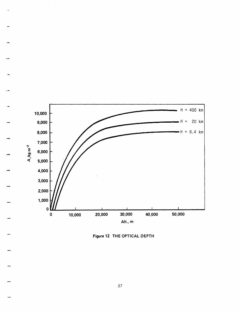
10,000
9,000
8,000
7,000
E 6,0006,000
< 5,000
4,000
3,000
2,000
1,000
0
0 10,000 20,000 30,000 40,0(
Alt., m
Figure 12 THE OPTICAL DEPTH
37
)0 50,000
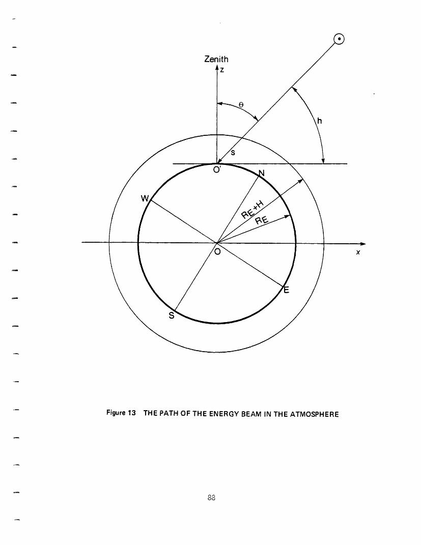
Zenith
x
Figure 13 THE PATH OF THE ENERGY BEAM IN THE ATMOSPHERE
88
CHAPTER 5
CORRELATION OF THE SOLAR ENERGY RADIATIVE FLUX DEPLETION WITHMETEOROLOGICAL CONDITIONS
This chapter will develop the concepts and techniques
needed to compute those coefficients of eq. 4.35 that are
dependent on meteorological conditions.
A macro- and microclimatic approximation for each
coefficient of eq. 4.35 will be considered. Consequently, a
mesoclimatic approximation will be defined.
The purpose of a macroclimatic approximation is to derive
the energy flux values within "Standard Climatic Areas," for
techno-economical feasibility studies of solar energy
applications.
It is assumed, for these purposes, that no meteorological
data are available.
The mesoclimatic approximation will reduce the "Standard
Climatic Areas" to a relatively narrow zone, for which only
standard meteorological data are available (i.e., pressure,
temperature, and dew point or relative humidity), plus some
89
information on the clouds (i.e., main cloud type or cloud
layer, percent of dome covered by clouds, or minutes of
sunshine)--this information being furnished on a daily average
basis. This approximation will serve the engineering
optimization of the solar energy conversion systems.
The microclimatic approximation will assume that local
meteorological data are measured at the site under
consideration, on an hourly basis--or at least a few times a
day--and that some precise information on the clouds is
available. This will allow solar maps of those regions that
have good records, and/or a history of "standard"
meteorological data that are absolutely unrelated to solar
energy flux measurements.
The main criteria of this chapter will be:
i. to obtain the maximum precision of the correlation
through a physical model, but
ii. to avoid those extremely precise physical models
that, although they might theoretically be constructed, will be
in high contrast with the amount and the quality of
meteorological data "generally" available.
90
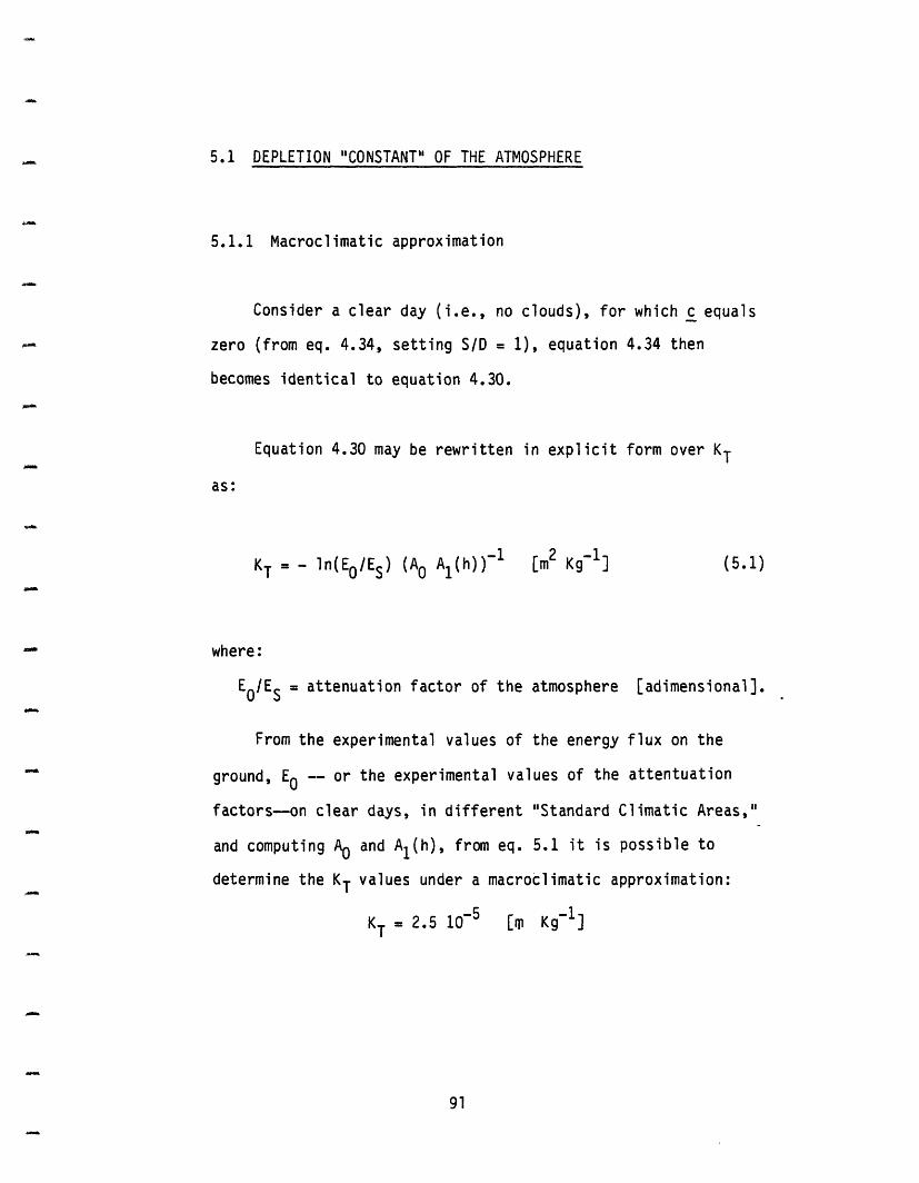
5.1 DEPLETION "CONSTANT" OF THE ATMOSPHERE
5.1.1 Macroclimatic approximation
Consider a clear day (i.e., no clouds), for which c equals
zero (from eq. 4.34, setting S/D = 1), equation 4.34 then
becomes identical to equation 4.30.
Equation 4.30 may be rewritten in explicit form over KT
as:
KT =- ln(EO/Es) (AO Al(h))-1 [m2 Kg-l] (5.1)
where:
E0/ES = attenuation factor of the atmosphere [adimensional].
From the experimental values of the energy flux on the
ground, E0 -- or the experimental values of the attentuation
factors--on clear days, in different "Standard Climatic Areas,"
and computing A0 and A(h), from eq. 5.1 it is possible to
determine the KT values under a macroclimatic approximation:
KT = 2.5 10 5 [ Kg-1]
91
for temperate winter, continental climatic conditions or desert
climates (particularly clear atmosphere and low level of
humidity);
KT = 3.0 10-5 [m2 Kg- 1]
for temperate summer, continental climatic conditions (clear
atmosphere and medium level of humidity);
KT = 3.5 10-5 [m2 Kg - 1]
for humid (tropical) climatic conditions (clear atmosphere and
high level of humidity).
It would not make sense, under this approximation, to
determine whether those KT values refer to the global or
direct attenuation, since they are largely obtained through
averaged meteorological conditions.
Particular polluting agents, such as dusts, haze, fog,
smoke, etc., will cause a substantial increase of KT
(approximately, .6 10-5 in particularly critical
conditions). Therefore, the range of variation of KT is from
2.3 10-5 to 4.2 10-5.
92
The computed KT values appear to present a very low
sensitivity with respect to the solar altitude; this confirms
the methodology adopted for the relative atmospheric mass
computation and the value chosen to be the height of the
atmosphere for this computation.
On the other hand, KT does have a dependency with respect
to the clouds' presence and this fact is independent of the
clouds' absorbance.
Using eq. 4.35, which gives the density of energy flux on
a cloudy day, a better approximation is obtained if the KT
values previously defined are correlated to the clouds'
presence through the following empirical relation, which takes
into account the clouds' absorbance and the increase in water
vapor in the atmosphere due to the clouds' presence:
KT = KT (1 + .3 n) [m Kg ] (5.2)
Equation 5.2 states that, in the presence of clouds, KT is
increased by a quantity linearly proportional both to the
clouds' quantity and KT itself (up to a maximum value of
1.2 KT), and KT is consequently defined. The constant of
proportionality has been empirically determined, at this stage
on a large macroclimatic approximation.
93
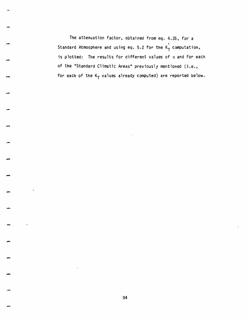
The attenuation factor, obtained from eq. 4.35, for a
Standard Atmosphere and using eq. 5.2 for the KT computation,
is plotted: The results for different values of n and for each
of the "Standard Climatic Areas" previously mentioned (i.e.,
for each of the KT values already computed) are reported below.
-.3
94
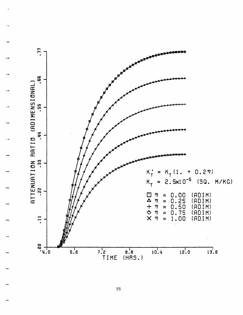
TIME (HRS.)
95
-j
C:z
z
C:I-
C:
zU!--
(3
cDto
rD
,L
r)
u13
cj
'-
M/KG)
12.0 .6--
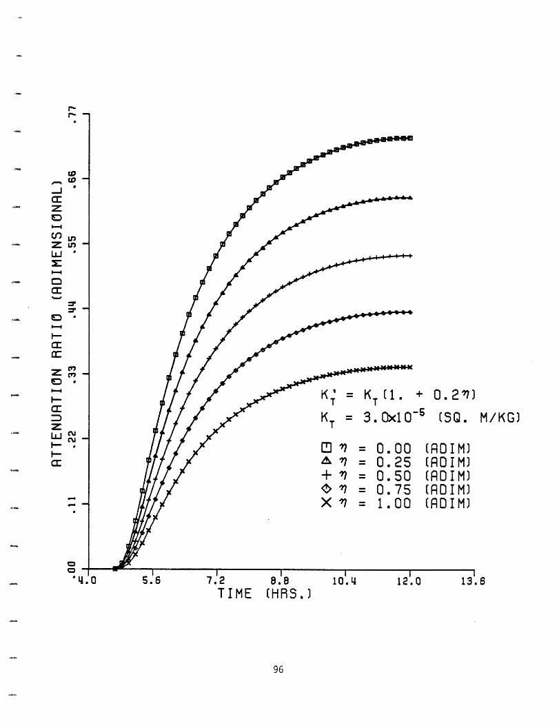
r,-
C-z
LU
a:n:
zLLJ
COCD
=4
=4
C,,C,
CuCU
K = KT (1 + 0. 2?)
K T = 3.xl10- 5 (SQ.
E 7 = 0.00 (RDIM)A 1 = 0. 25 (ROIM)+ Xl = 0.50 (ROIM)< X = 0.75 RODIM)X 7 = 1.00 (RDIM)
TIME HRS.
96
M/KG)
oo
6
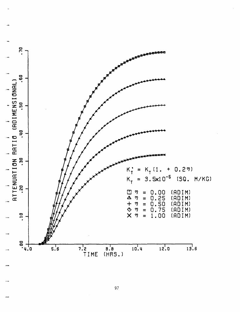
K = KT (1. + 0.281)
KT = 3.5x10- 5 (SQ.
Cl '1 = 0.00 (RDIM)A 7 = 0.25 [(RDIM)+ '1 = 0.50 (ROIM)< 1 = 0.75 (RDIM)X X = 1.00 (RDIM)
0TIME (HRS,)
97
CD0,
0to
0U,)CD
CZan
CDcr
TO(rD
TO
-
-
-4I--C
zLr Vz---
c:
M/KG)
0. I ,6
5.1.2 Microclimatic approximation
For a meso- or microclimatic approximation, the KT
computation should be strictly related, in an explicit form, to
the meteorological parameters.
It is evident that the number of parameters considered may
be as high as required. Theoretically, since those
parameters-here called meteorological parameters (to enhance
their dependency with respect to time and location)--are
nothing more than all those factors that qualitatively and
quantitatively describe the components of the atmosphere as
concerns their interaction with the electromagnetic beam, the
higher the number of factors considered, the higher will be the
precision of the model.
Nevertheless, in order to be able to use a physical model,
all the parameters considered should be determined and,
obviously, determinable. Furthermore, their measurement should
generally be already available (e.g., because data have been
developed for other purposes), or at least, they should be
determinable (by computation or measurement) in a relatively
simple and economic way.
98
Records of meteorological data are extremely rare,
incomplete, and imprecise. It has been noticed, trying
different methodologies of correlation, that relatively
complete physical models are rather sensitive to a lack of
strong approximation on the values of the input data needed.
They often appear to be less precise, even drastically so, than
simpler models for which the input data are available with a
certain precision and extension.
Therefore, a general criterion for the microclimatic
correlation has beeneadopted: implement as complete a model as
possible but keep it always compatible with the meteorological
input data "generally" available. This is rather hard to
accomplish with clouds, as concerns the availability and
significance of data, or for the amount of water vapor present
in the atmosphere, as concerns the complexity, precision, and
cost of necessary measurements. In these cases, the simplest
possible approach has been used, and alternative ways of
computation have been indicated, even when they imply an
appreciable drop in precision.
With these criteria in mind, KT will be expressed as a
function of the standard components of the atmosphere, i.e.,
permanent gases, amount of water, and amount of polluting
agents and dispersers, such as haze, fog, dust, etc. Thus:
99
K T = KT (standard components, water vapor, local factors)
The following form will be used:
P3KT = P1 + P2 w + P4 p (5.3)
where:
p1 = depletion due to permanent components of the
atmospheric gas (N2, 02, Ar, 03, etc.)
w = amount of precipitable water
P2 = intensive factor of depletion due to precipi
water
P3 = intensive factor of depletion due to precipi
water
P4 = intensive factor of depletion due to "local"
p = extensive factor representing depletion due
"local" factors.
table
table
factors
to
It is well known [47-49] (see Chapter 3) that water
vapor exerts a considerable influence on atmospheric
absorbance, and therefore on the radiative energy flux
depletion. A nonlinear dependence of KT with respect to the
water vapor present in the atmosphere has been found, as may be
seen from the following tabulation, obtained for S/D = 1 and no
"pollution" [50]:
100
A_
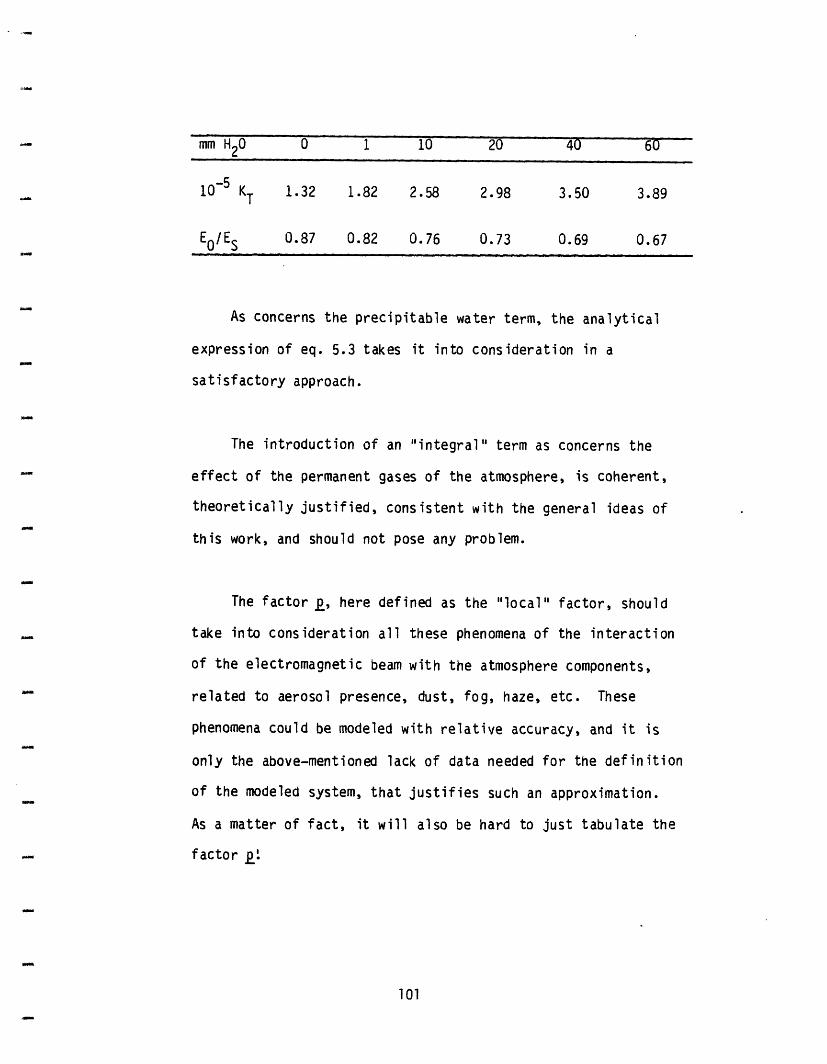
mm H20 0 1 10 20 40 60
10 5 KT 1.32 1.82 2.58 2.98 3.50 3.89
Eo/ES 0.87 0.82 0.76 0.73 0.69 0.67....................... ~~~~~
As concerns the precipitable water term, the analytical
expression of eq. 5.3 takes it into consideration in a
satisfactory approach.
The introduction of an "integral" term as concerns the
effect of the permanent gases of the atmosphere, is coherent,
theoretically justified, consistent with the general ideas of
this work, and should not pose any problem.
The factor p, here defined as the "local" factor, should
take into consideration all these phenomena of the interaction
of the electromagnetic beam with the atmosphere components,
related to aerosol presence, dust, fog, haze, etc. These
phenomena could be modeled with relative accuracy, and it is
only the above-mentioned lack of data needed for the definition
of the modeled system, that justifies such an approximation.
As a matter of fact, it will also be hard to just tabulate the
factor .
101
Both the form and the parameters considered in eq. 5.3
permit the obtaining of a satisfactory relation between KT
and the atmospheric parameters. This relation is believed to
be the most precise and realistic obtainable, considering the
meteorological data records "generally" available.
Furthermore, it appears to be quite independent from the
geographic location to which it is applied, thus showing a
physical content and a non- (totally) empirical formulation.
The integral transparency coefficient for a dry and clean
atmosphere on a clear day with no clouds is known to be:
after Kastrov [51-52] 0.910
International Radiation Commission (1956) 0.915
after Sivkov [53] 0.907
Recalling the definition of the integral transparency
coefficient from eqs. 4.26 and 4.29, and setting w and p equal
to zero in eq. 5.3, the factor P1 may be easily computed (or
verified).
Once P1 has been obtained, considering a real atmosphere
on a particular clear day with no clouds or polluting agents,
recalling eq. 4.29, assuming p equals zero, the factors P2
and p3 are obtained, using a best-fitting procedure
(least-square regression technique).
102
For the moment, and on a first approximation, eq. 5.3 will
be considered without the "pollution" (or "local") factor p.
Under these circumstances, eq. 5.3 may be rewritten as:
-5 .40 2K-(.40)K = 10-5 (1.00 + .40 w 40) [m Kg- (5.4)
where the amount of precipitable water is expressed in
millimeters, and p2 and p3 values correspond to a smooth
best-fitting, accomplished with southern European data.
Measured values of precipitable water for the U.S. are
available on the basis of two balloon measurements per day, at
0.00 and 12.00 hours, G.M.T. The basic raw data generally up
to 500 mbars, needs to be elaborated and, sometimes,
extrapolated (or multiplied by a 1.15 factor). An alternative
way to compute the amount of precipitable water from pressure,
dew point (or relative humidity), and temperature values, using
the Clausius-Clapeyron equation and elementary concepts of
physics of the atmosphere, is reported in Appendix A3.
The sensitivity analysis of KT with respect to the three
parameters, pi, P2 and p3, using the "spider" graph technique,
is reported below for different values of w.
103
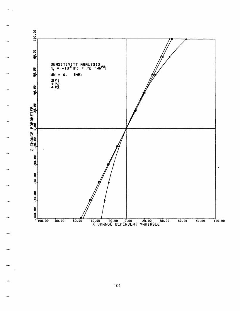
104
Oa
00
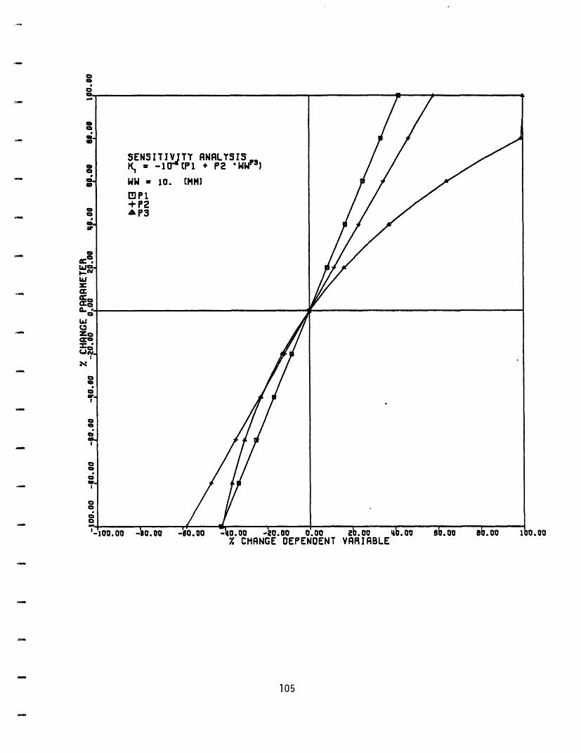
105
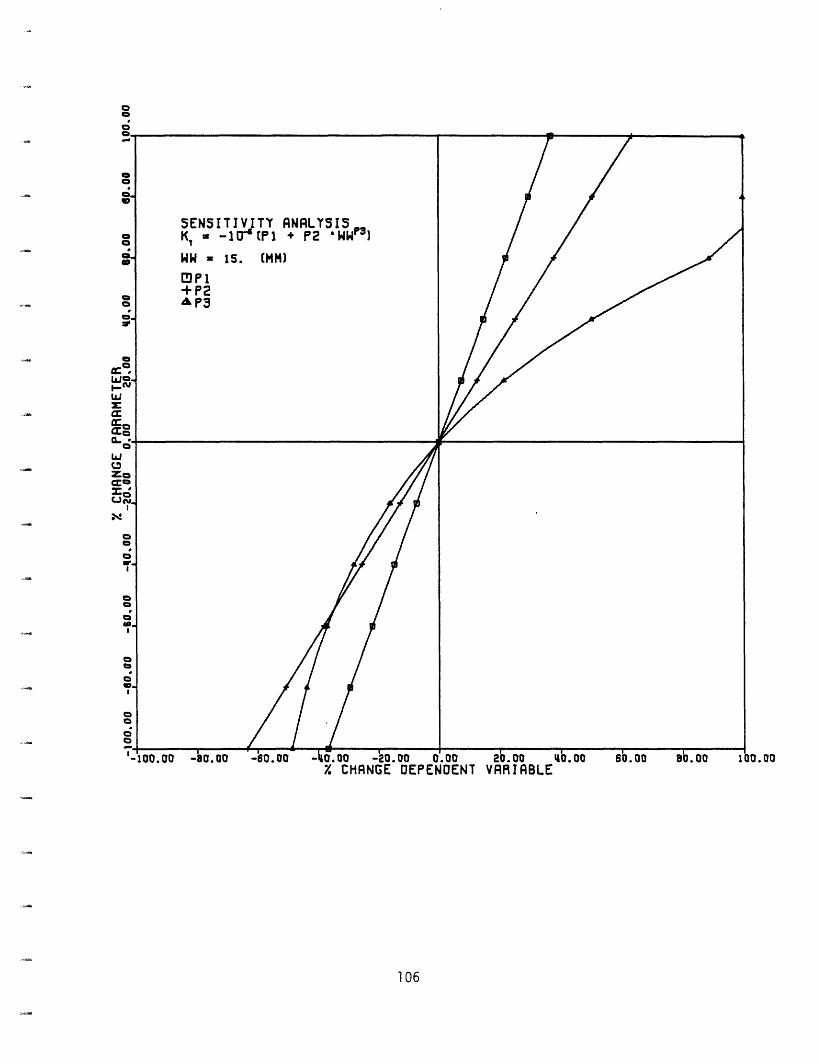
106
0CD
.00
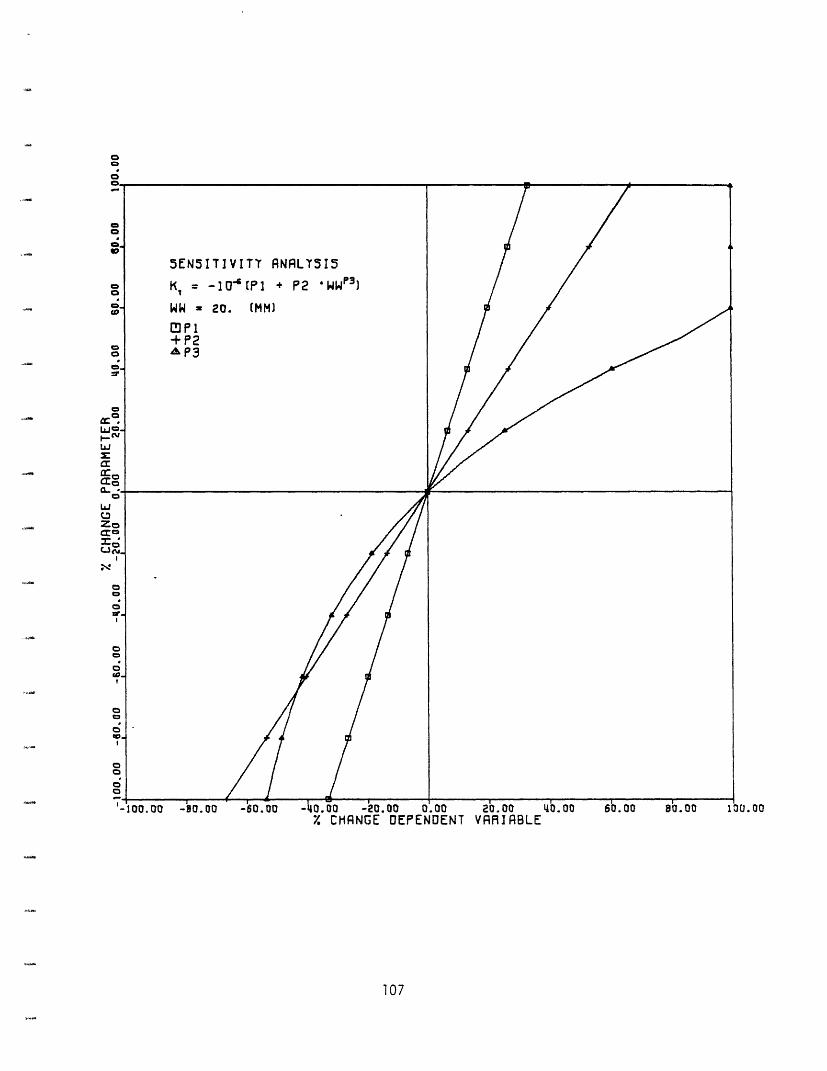
107
0C
.00
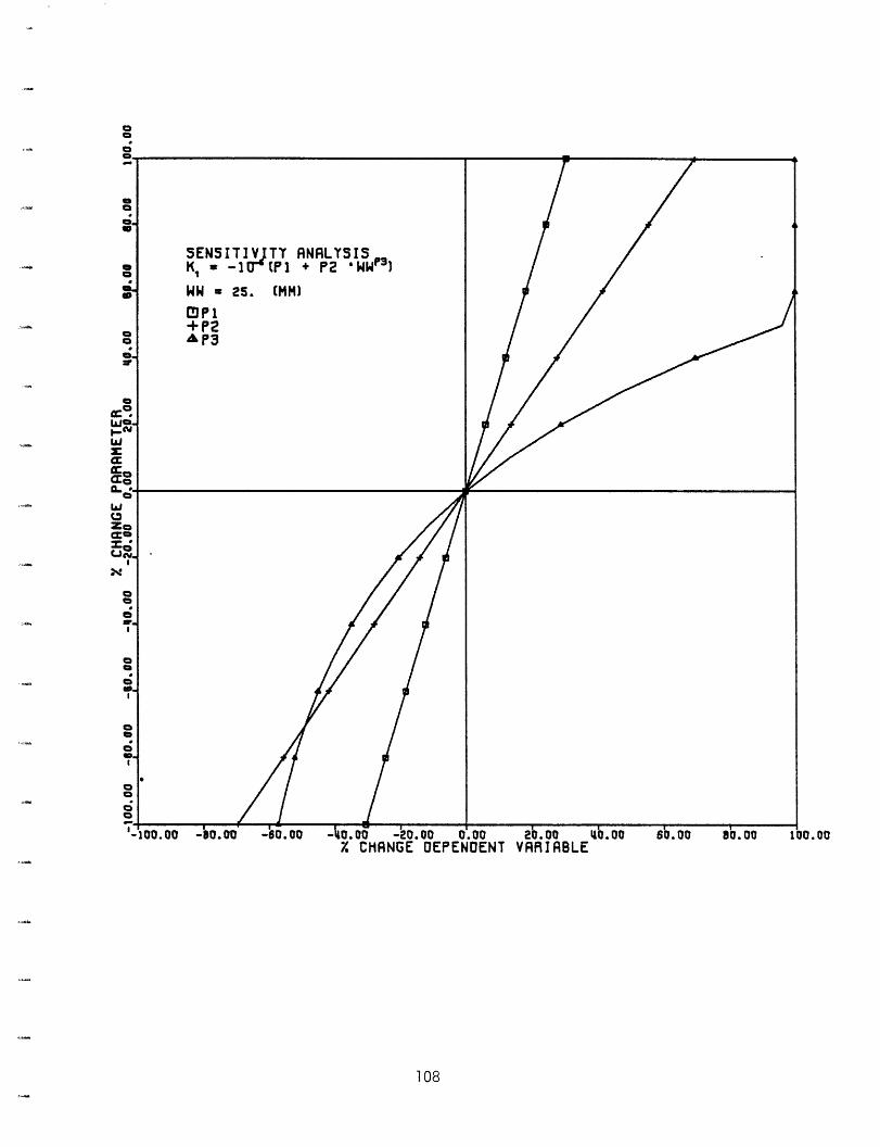
108
dl
00
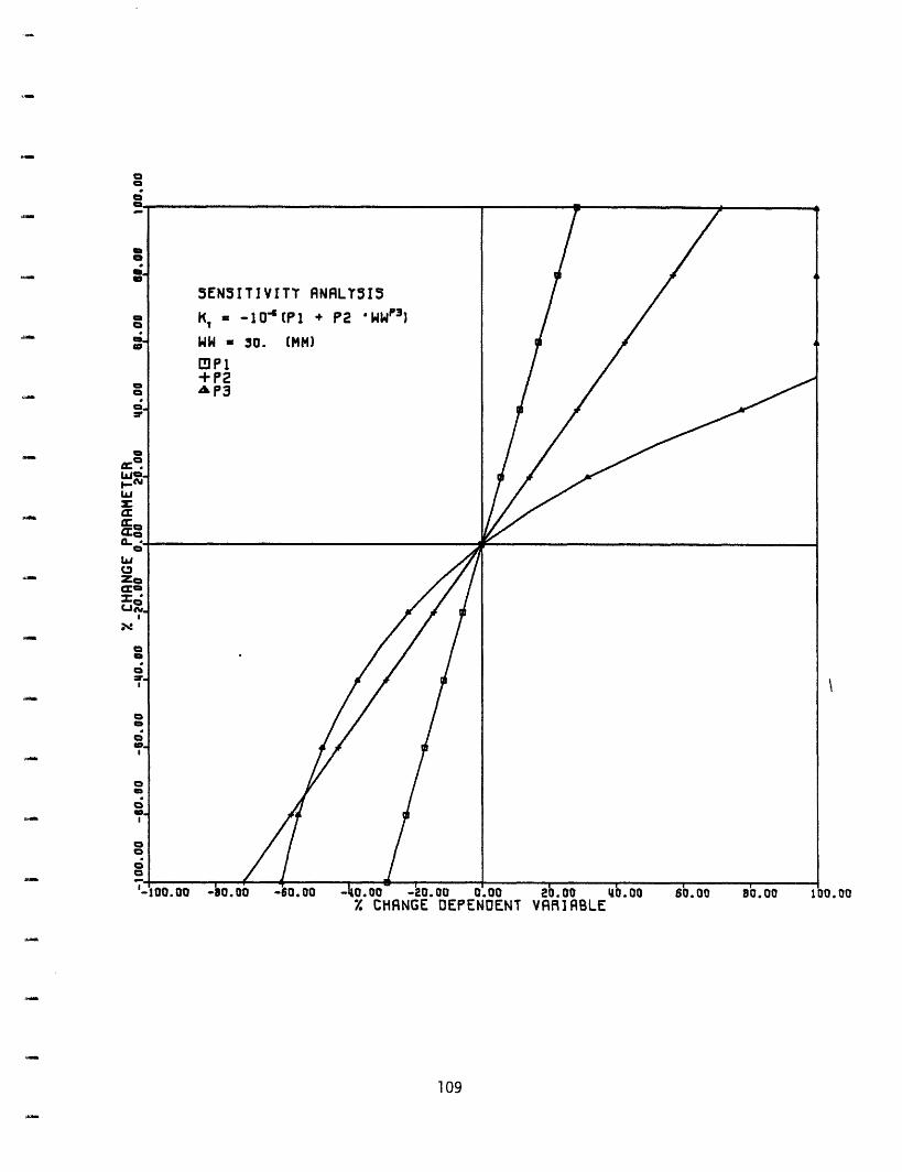
0a
109
Taking into consideration the explicit form of KT (given
in eq. 5.4), eq. 4.30, which computes the energy flux density
for noncloudy days, may be rewritten as:
E = E5 exp[- (10-5( 1. + .4 w'4) A0 A1(h))] (5.5)
A self-explanatory example output of the E computation,
following eq. 5.5, is reported below.
110
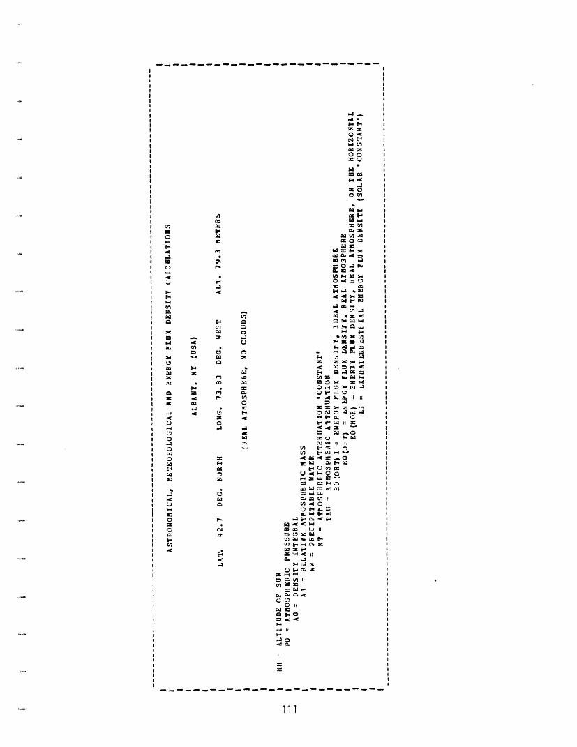
U,
;
543c;et
01r:
54-C
U,I-i 1U,
3:
m O>4 E 3
.i- WIIfa2 rI X.
4 . wr
Z* r3 54_4 C
0 L~~~~~'' .
E-
t;C C
54
w
raj0
i,*
_iH a'
,U, a04"I
C
a'E~in
_ O
11E-a'.5
1i
Ui
u04H
aa
U,
).
u II2t
i
* e
-CI
N Ho 2
00t4 Ek
cn
20 b
C2t^,'
ii O:a3:
-
4 E w
74 4 .4J-I ?4 IfefE-1 U U, Y
En2 1L.4 aHc rY '
54 tnr o _a X
WI E-4 -
m C ~- P z .r
2u E.41.
F- I .
5.4 H C.E- Eclr rm > C3 Z _
,4Me r a t>,
H0 0
:3J2z >sz tr lia W1 _ ZU Ektw H 12.z
a40,
H0
rII EiN U I =i r;i
:33
111
r,A02
-4-a
'.5Et I>4
-4iU,
->4J
'.
0r..
H31a
0_i0aCz
.
.4
~Ii0.4
0
20
W_itwr.3
z0
E:0-C
I
IIIIIIIIIIIIII
IIIIII
I
IIII
IIIIIIIII
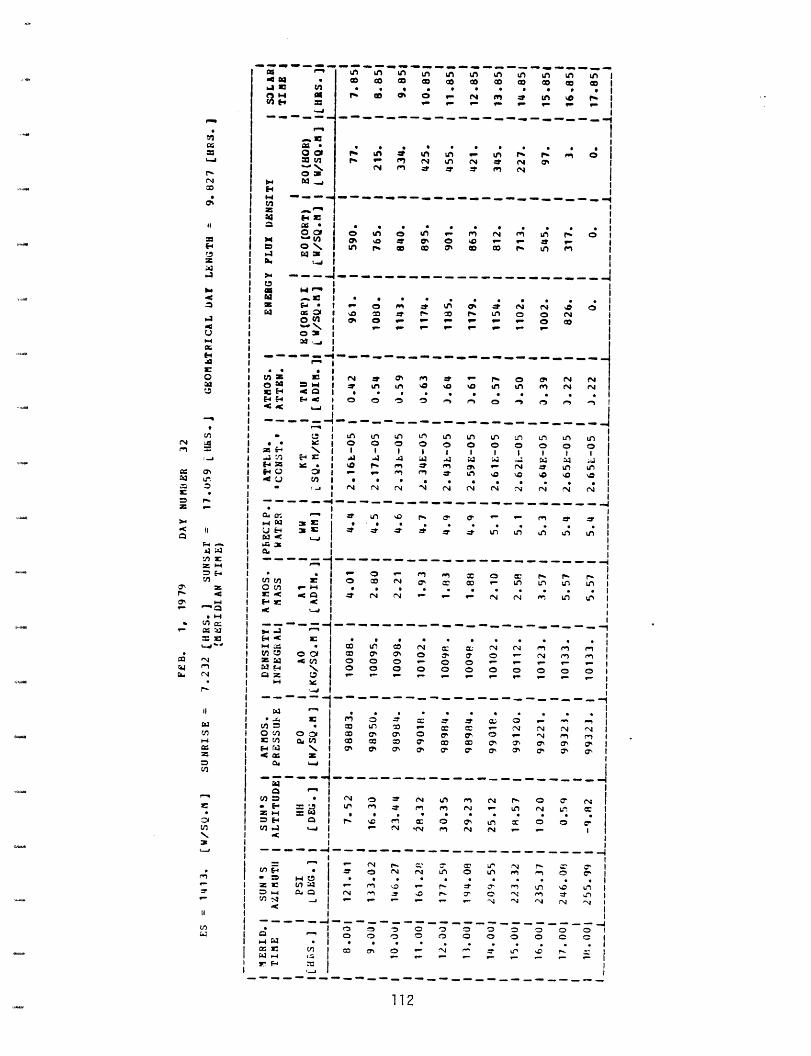
43-4 94
a:
r4l
3 Co
I 4 Y. ·3 > Oc
03 3
oaI a O
I D O 1 4 :
O t
If ·,_ _
1 u) WI LA LA tn LA Ln Ln LA L0 0 0 0 0 0 0 0 0 0 0
* * * * * * * * @ * S0v eD 0 O _ N :t IA %0
* LA * A LA LA t% L 9 0 - C N UL N :r N 0
O N O U* _ f9 N !
A Io co G % 0 0 o _ - LA 19
0- 9 9 - LA 0 *1 (N (N 4 O 010 I - a0 r. UlA 0 a0I % 0 . 0 -* . * *- *- 0 0
I ~ -O 0_ - 0- .- - 0- O _ _ _ __ _ _
I~ d i~r fI(b Clba~nr
I -_ _ _- _- _- _, _- _ _ _- -_
I i
I I * C * (I * - - C 0% N (NI = I N t LA ro o 0 L O 19 N NI E.4 .C I *..
I F4 C4 F g o o-1 o- -.% els C -5 e5 1. -I . I a C 3 : CI II - ----- - - -
' z m ,* I N A I , . bc,_ = I z E- -
0 I -I
L L n A L L L ( L LA L A
I n r e - r II
I * * L * * * * 0
,N N N N N N fN N 4 4 N
* * * * * * LA LA LA LUl ID F, , a, M _.NI.
0- 0 '~ In on X 0 0 e- F- eI - - 0% 0 W- LA LA LA LA 1
zr N tNJ tN ts9 tr 4 tq (
_ _ _ _ _ _ _ _ ~ _ m _ ~ _ b _ - _ _ _ ~ _ _O~N~_ - _ _
% 0 00 ;0 -' t N x ' o0
0o 000 0, 0 0 0 0 '
D0 ' N e N N -0* . 0 * * A *0 0 . *
r- ~ :, - W ul l- C
J 6 N N~~~~~~~O~~~~~~n b F ~ ~ z
co cm -2,.r I--,)
��������������---�----_-_-__
r.
If0
CH13
W. 3
.3
aIC13Z
= .b..-C 1
M P.
cia .0.4 4 o '3
W -W - 1-
Inr
v,
a, i-
3 H
=W
,_J -'
1:
,I
W
m
0-4
W.
V)
01
L'"I
L4 2;0 LnV C
t3 FA1
Q 3
0 cn
W4
Q.
En3
r4
11
---i-
cm E-4. = -4 0= IC En
~--- 44
= v: (W -4 F'. 4
112
Recalling that eq. 5.5 furnishes the value of the density
of energy flux (watts per square meter), the density of energy
flux on the horizontal (Lambert's Law) can be directly derived:
E = ES exp[- KT AO Al(h)] cos(6) (5.6)
where:
e = angle between the beam's direction and the normal to
the surface being considered (often called zenith
angle)
It should be noted, as concerns eq. 5.6, that as concerns
the horizontal surface, the normal to the surface coincides
with the zenith; recalling the definition of the altitude of
the Sun, h (see Chapter 2), it is immediately seen that the
altitude and the zenith are complementary angles. Thus, and
only for the horizontal plane:
cos(e) = sin(h) (5.7)
The symbol E0 has been extensively used throughout this
work to represent a density of energy flux; therefore the same
symbol will be used when computing the density of energy flux
for any surface. This implies a slight alteration in the
physical meaning of the vector energy flux density, since the
113
flux density of a vectorial magnitude is always computed
through a surface perpendicular to the vector.
The "spider" technique sensitivity analysis is applied to
eqs. 5.6 and 5.5, using the expression of KT furnished by eq.
5.4, and the E0 sensitivity is analyzed with respect to the
atmospheric pressure and the amount of precipitable water
values (the first independent variable will affect the A0
computation--density integral; the latter will affect the KT
computation--atmospheric attenuation "constant") for four
different hours of the day. The results are reported below,
both for E on the horizontal (eq. 5.6) (energy flux density on
the horizontal) and E0 ortogonal to the beam's direction (eq.
5.5) (energy flux density).
114
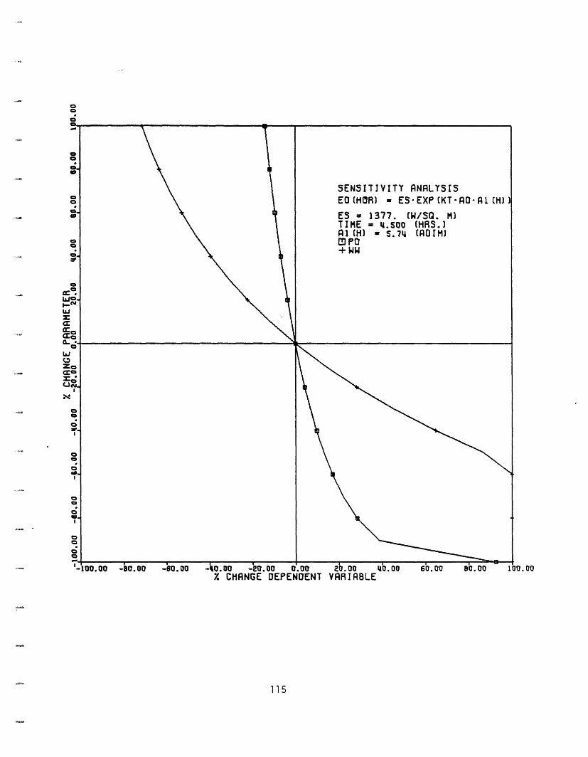
115
CC
00
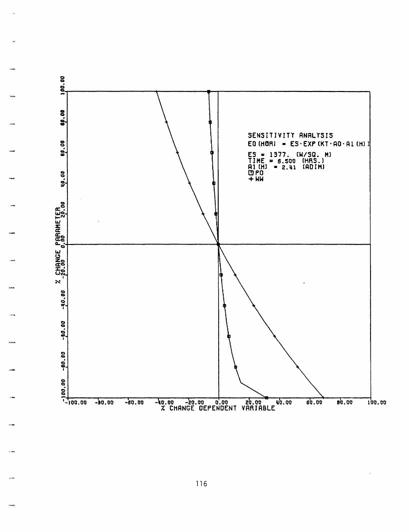
OCa
116
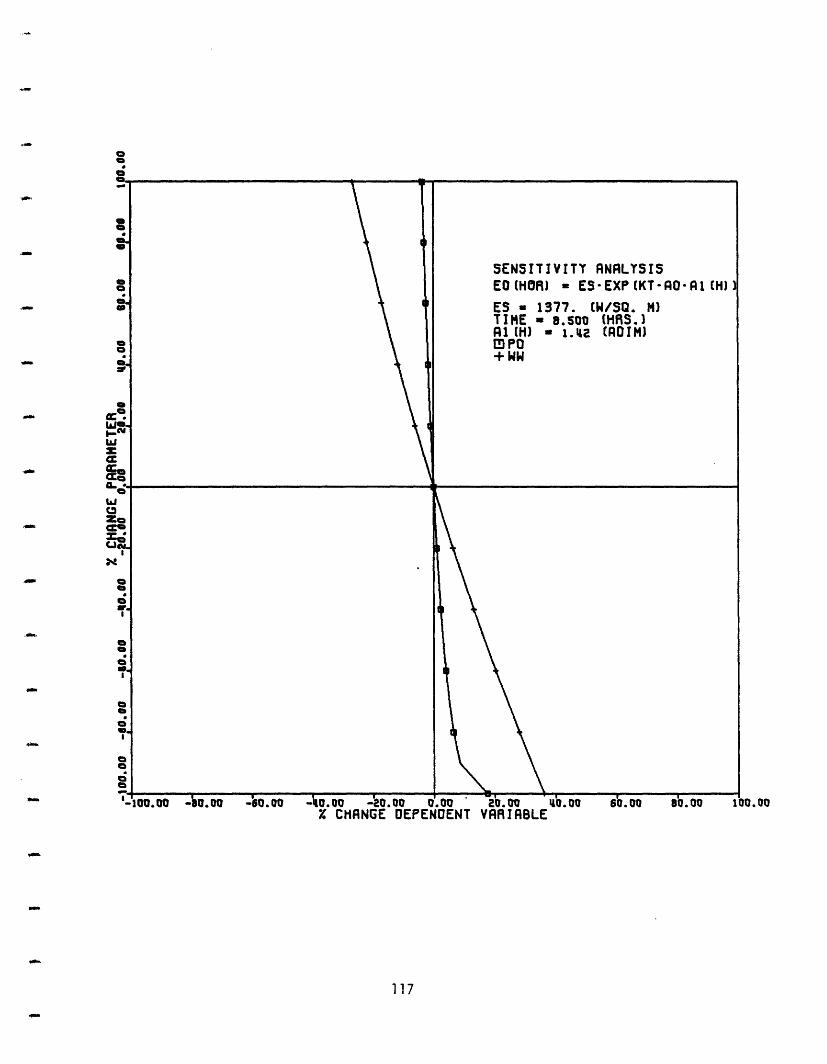
117
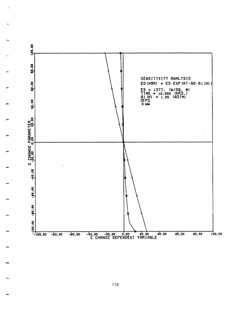
.00
118
oII
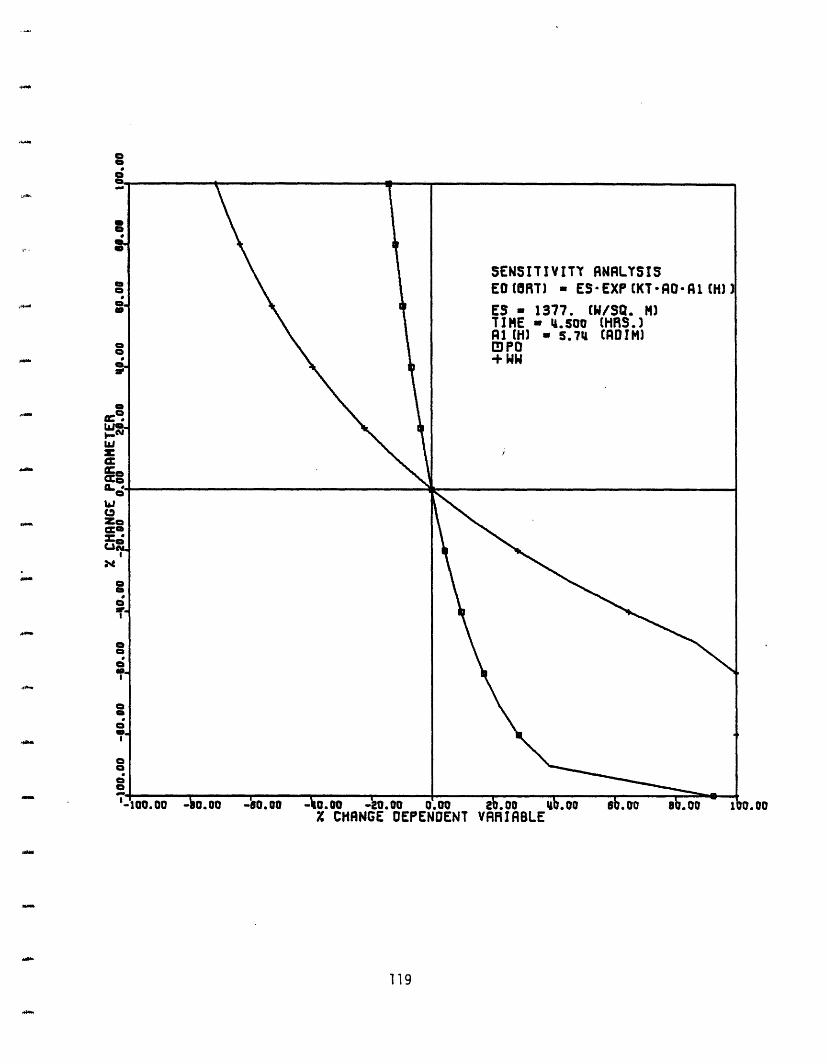
119
-
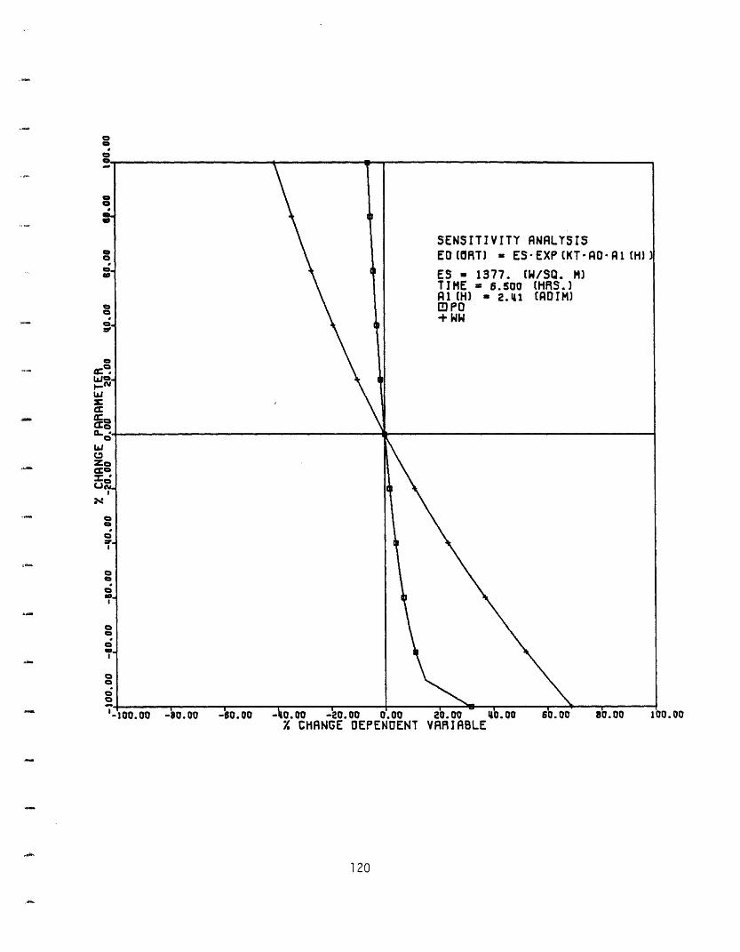
0a
120
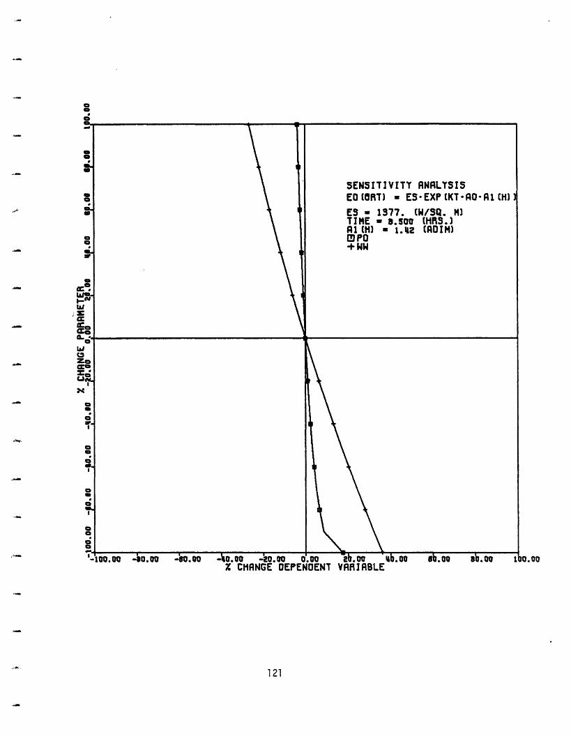
.00
121
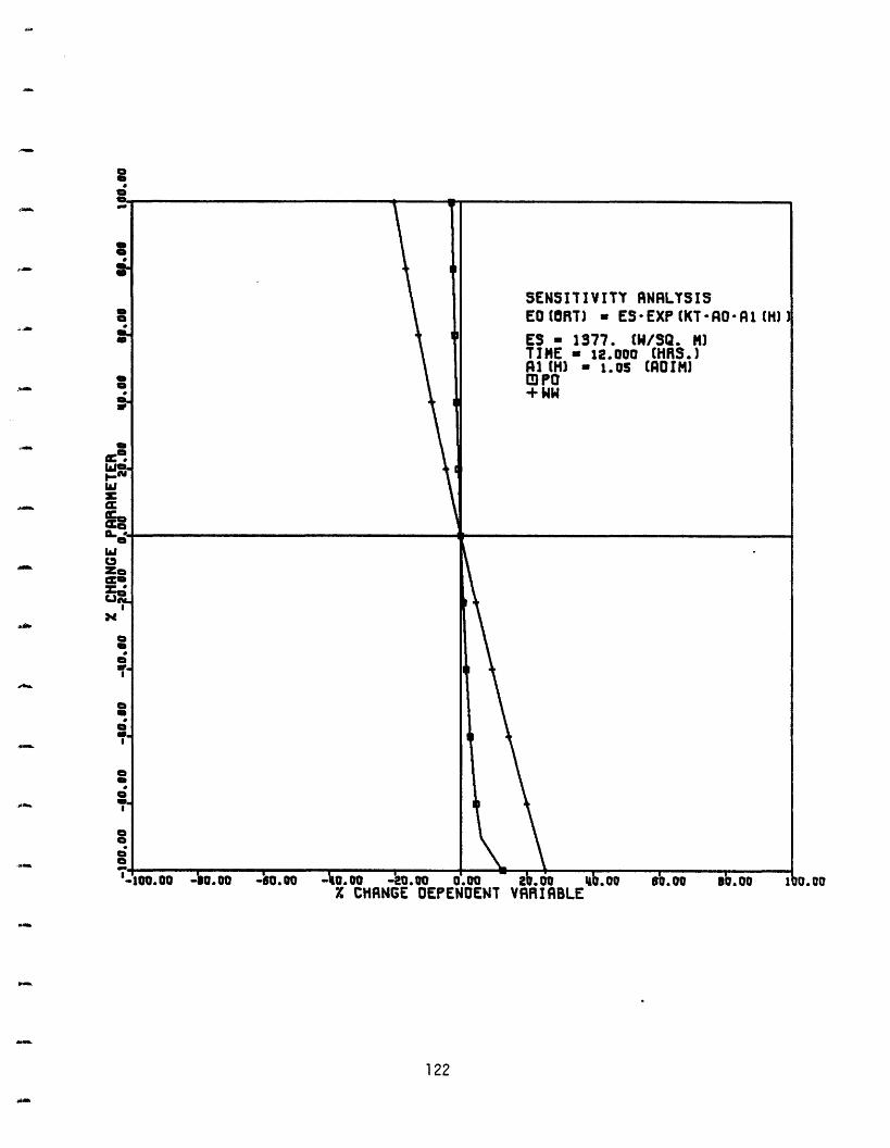
122
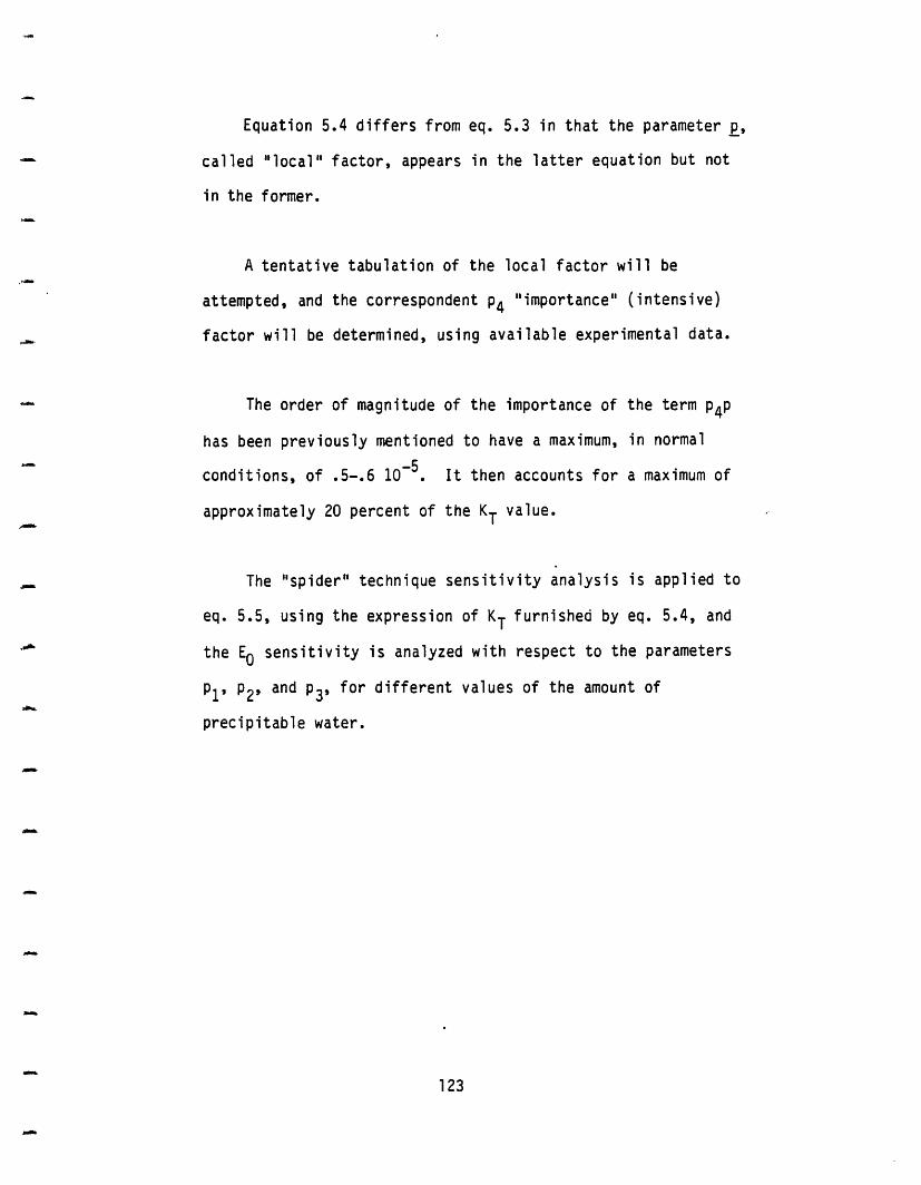
Equation 5.4 differs from eq. 5.3 in that the parameter p,
called "local" factor, appears in the latter equation but not
in the former.
A tentative tabulation of the local factor will be
attempted, and the correspondent p4 "importance" (intensive)
factor will be determined, using available experimental data.
The order of magnitude of the importance of the term p4p
has been previously mentioned to have a maximum, in normal
conditions, of .5-.6 10-5 . It then accounts for a maximum of
approximately 20 percent of the KT value.
The "spider" technique sensitivity analysis is applied to
eq. 5.5, using the expression of KT furnished by eq. 5.4, and
the E sensitivity is analyzed with respect to the parameters
P1, P2, and P3, for different values of the amount of
precipitable water.
123
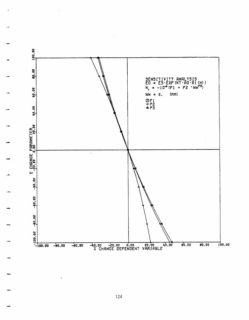
124
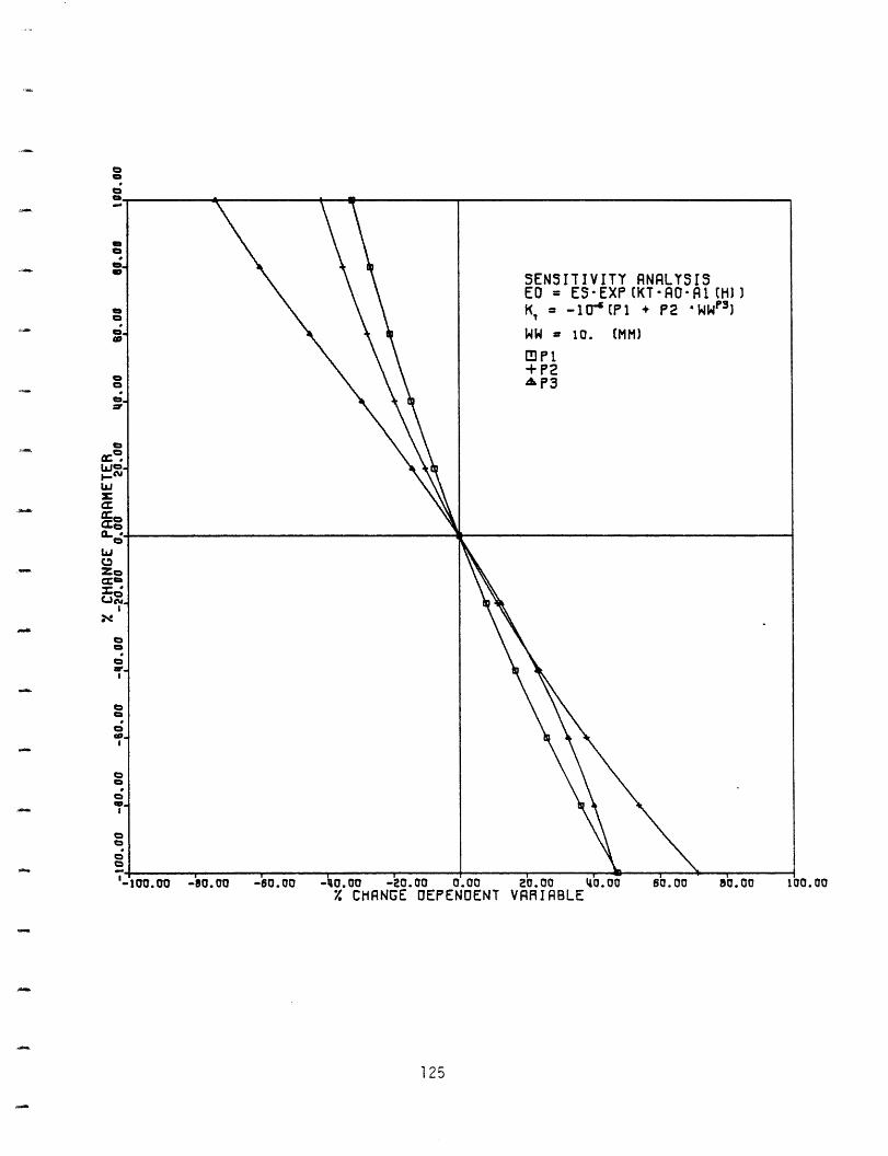
o00
125
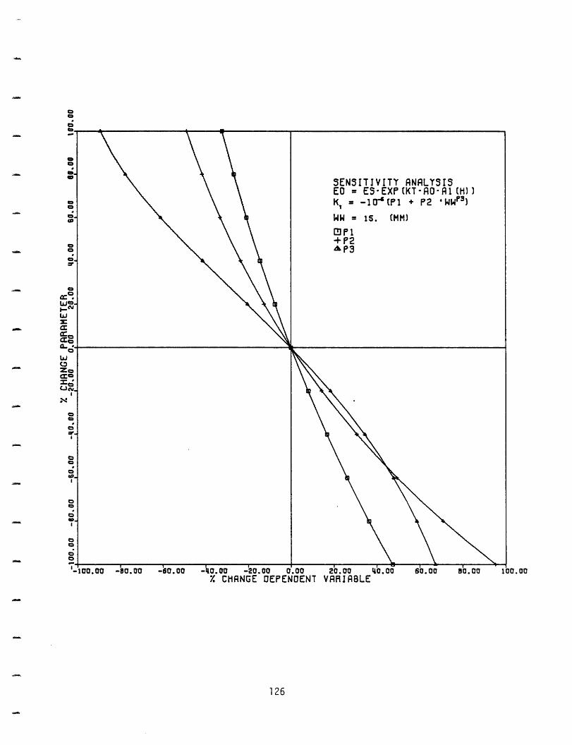
126
COC
00
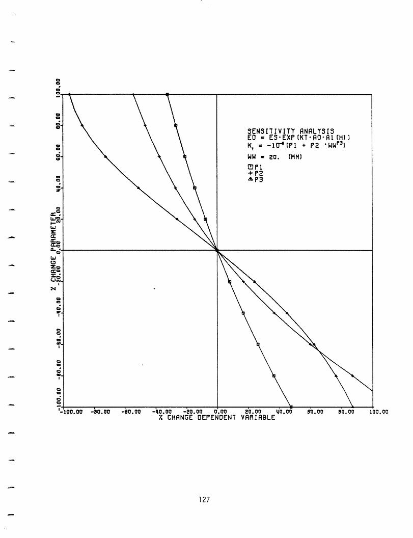
00o
127
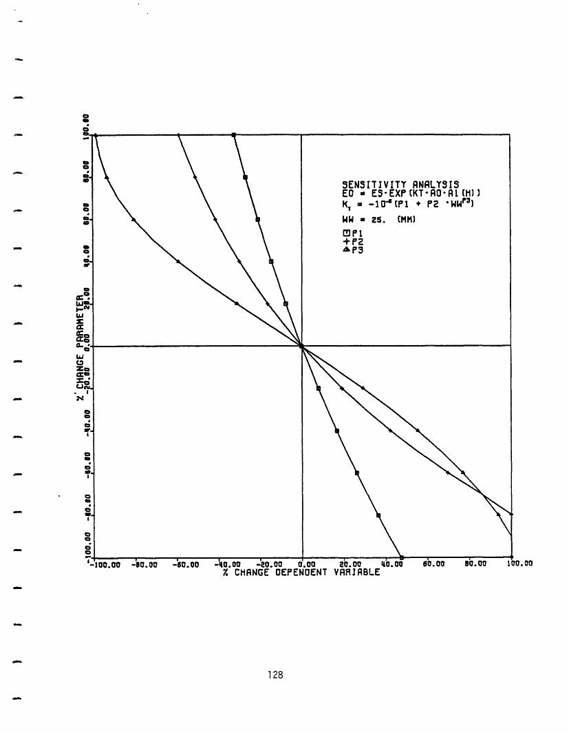
00
128
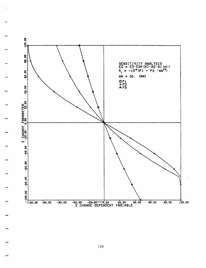
i-100.00 -80.00 -60.00 00
129
5.2 QUANTITATIVE ASPECTS OF THE CLOUD PRESENCE
The dynamics of the interaction between the
electromagnetic radiation and the clouds have been described in
Chapter 3. There it was stressed that, as large particles are
strong light scatterers, the clouds strongly deplete the
radiation beam through diffusion (and absorption).
It has also been pointed out how a "differential"
(punctual) approach to this interaction, in order to construct
a physical model of the interaction itself, was almost
impossible to accomplish.
Therefore, an "integral" approach, through an intensive
factor (albedo) and an extensive factor (minutes of sunshine
per interval of time), as deep as the available measured data
allowed, has been attempted.
It should be stressed that the clouds' presence strongly
affects the precision of any model, even assuming that a
sensible amount of data on the clouds are available.
5.2.1 Macroclimatic approximation [54]
Worldwide, cloud cover is maximum at high latitudes and in
the tropics, and minimum in the subtropics. The global mean
130
albedo is 0.31 and the global mean cloud cover is 0.53. These
values are quoted only as reference, but clearly cannot be
adopted in any model. More precise data, quarterly and for
"Standard Climatic Areas," are available and should be used for
largely approximated computations [55-59].
The measurement of the minutes of sunshine per interval
time may be a particularly simple relevation and, generally,
predominant cloud types, for every region and climatic area,
are available for many locations. Computing albedo as
indicated in the next section, with the accuracy permitted by
the available data, more realistic computations may be
achieved, using eq. 4.35 and the macroclimatic values of KT
furnished in Subsection 5.2.1.
5.2.2 Microclimatic approximation l
Cloud information, although aleatory, is generally
available; most measurement techniques and terminology have
been determined by the world Meteorological Organization. This
is due to the great interest that meteorologists have in
climate models. Since one of the fundamental climatic
variables is the global mean temperature, which depends on the
global albedo, an important part of which depends itself on the
clouds, a relatively complete set of cloud data is "generally"
available.
131
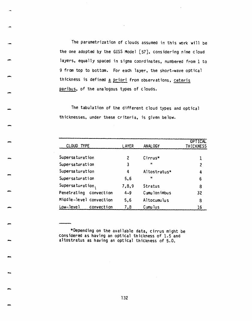
The parametrization of clouds assumed in this work will be
the one adopted by the GISS Model [57], considering nine cloud
layers, equally spaced in sigma coordinates, numbered from 1 to
9 from top to bottom. For each layer, the short-wave optical
thickness is defined a priori from observations, ceteris
paribus, of the analogous types of clouds.
The tabulation of the different cloud types and optical
thicknesses, under these criteria, is given below.
OPTICALCLOUD TYPE LAYER ANALOGY THICKNESS
Supersaturation 2 Cirrus* 1Supersaturation 3 " 2Supersaturation 4 Altostratus* 4Supersaturation 5,6 " 6Supersaturation\ 7,8,9 Stratus 8
Penetrating convection 4-9 Cumulonimbus 32Middle-level convection 5,6 Altocumulus 8
Low-level convection 7,8 Cumulus 16
*Depending on the available data, cirrus might beconsidered as having an optical thickness of 1.5 andaltostratus as having an optical thickness of 5.0.
132
The albedo for the various analogies of the different
cloud types* is computed from an approximate formula, based on
the scattering theory [60]:
a = 0.13 T/(1 + 0.13 T) (5.8)
This is the parametrization used in ref. 57 on a
simulation of the January climatology, and the obtained results
appear to be realistic [55].
Therefore, once the optical thicknesses of the different
cloud types are derived from the previous tabulation, the cloud
albedo will be computed using eq. 5.8.**
The minutes of sunshine per interval time (or the percent
of the celestial dome covered by clouds--although this factor
gives a lower precision in the calculation) should be known on
an hourly or, at least, on a daily basis. The n factor is
*From now on the "Analogies" of the previous tabulationwill be defined as "cloud types."
**The information needed under this hypothesis ofcalculation is--or will be--furnished by the data recorded onthe SOLMET tapes, prepared by the U.S. Department of Commerce,National Oceanic and Atmospheric Administration, EnvironmentalData and Information Service, National Climatic Center,Asheville, N.C., U.S.A. The analysis of the SOLMET data willbe discussed further in this chapter. This information isbeing furnished now only to give an idea of the availability ofthe required data.
133
particularly sensitive to the minutes of sunshine per interval
time information and, therefore, if the percent of sky cover is
used,-the minutes of sunshine should be known on an hourly
basis.
5.3 SOLMET - METEOROLOGICAL DATA
SOLMET tapes, both in FORTRAN and uniform format, furnish
records of solar radiation and "related" periodical (hourly or
tri-hourly) meteorological measurements in S.I. units [61,62].
Historical data are available, beginning in the early
1950s and ending in the mid-1970s. The data collection is not
complete and the amount of information varies from station to
station and with respect to time for each datum. It will be
complete, however, because SOLMET now retrieves data from the
"New National Weather Service network and cooperators." A
description of SOLMET data and relative format is reported in
Appendix A4.
Details on the acquisition systems are described in the
National Weather Service Observing Handbook No. 3, "Solar
Radiation Observations," here indicated as reference [63].
134
Due to incoherencies in calibration and problems in
instrumentation, only modeled ("regression" techniques) direct
hourly energy flux, from rehabilitated [64] observed hourly
hemispherical and hourly direct energy fluxes, are available,
at the moment, for 27 stations in the U.S. [65].
The meteorological data given in SOLMET tapes (see
Appendix A4) cover 222 stations in the United States. The
pressure, dry-bulb temperature and dew-point readings are made
every three hours. Pressure values are in kPa; they should be
converted into N m-2 (multiplying by a factor of 10);
temperatures are given in degrees Celsius, to be, if needed,
converted into degrees Kelvin (adding 273.16) or degrees
Rank ine).
As concerns the cloud cover and the clouds the SOLMET also
reports visual evaluations (see Appendix A4) of:
i. total sky cover, i.e., tenths of celestial dome
covered by clouds;
ii. total opaque sky cover, i.e., tenths of celestial
dome covered by clouds or obscuring phenomena through which the
sky or the higher cloud layers are invisible; and
iii. cloud types (14 different indexes, see Appendix A4)
and amount of clouds in tenths, for the visible part of each of
the four layers considered.
135
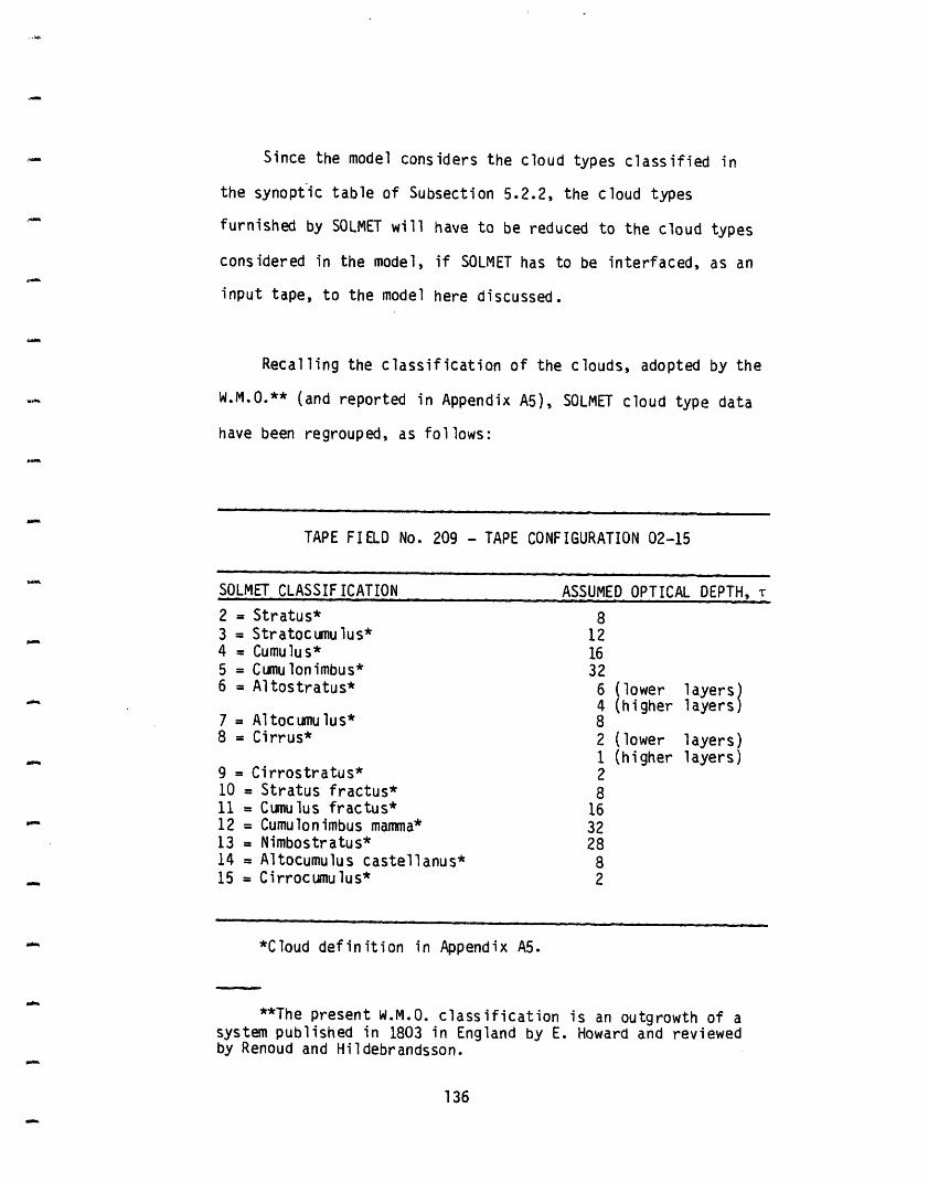
Since the model considers the cloud types classified in
the synoptic table of Subsection 5.2.2, the cloud types
furnished by SOLMET will have to be reduced to the cloud types
considered in the model, if SOLMET has to be interfaced, as an
input tape, to the model here discussed.
Recalling the classification of the clouds, adopted by the
W.M.O.** (and reported in Appendix A5), SOLMET cloud type data
have been regrouped, as follows:
TAPE FIELD No. 209 - TAPE CONFIGURATION 02-15
SOLMET CLASSIF ICATION
2 = Stratus*3 = Stratocumulus*4 = Cumulus*5 = Cumulonimbus*6 = Altostratus*
7 = Altocumulus*8 = Cirrus*
9 = Cirrostratus*10 = Stratus fractus*11 = Cumulus fractus*12 = Cumulonimbus mamma*13 = Nimbostratus*14 = Altocumulus castellanus*15 = Cirrocumulus*
ASSUMED OPTICAL DEPTH, T
81216326 (lower layers)4 (higher layers)82 (lower layers)1 (higher layers)2816322882
*Cloud definition in Appendix A5.
**The present W.M.O. classification is an outgrowth of asystem published in 1803 in England by E. Howard and reviewedby Renoud and Hildebrandsson.
136
, S
In the beginning of this section, it was stated that
SOLMET furnishes digitized meteorological data until
approximately 1975. The related solar data situation, however,
is somewhat critical, mainly in that values furnished have been
modeled or "massaged." Most of the available solar data for
the U.S. and for the period actually covered by SOLMET data
present this problem. This is clear if it is understood that
SOLMET tapes are a digitized source of practically all
available data, in logical or analogical form.
Post-1975 experimental values have not yet been
implemented in SOLMET format. They are available, though, in
an analogic form, from the U.S. Dept. of Commerce, N.O.A.A.,
National Weather Service as concerns all surface weather
observations, and through the New National Weather Service
network members or cooperators as concerns solar measurements
(accomplished following an improved, standardized, and strict
methodology).
In Appendix A6 the analogic data record format is
presented; this refers to the second sheet of the daily surface
weather observation records. A legend for reading and
interpreting the data is also furnished.
137
5.4 SUMMARY AND MODEL INPUT DATA
Since the availability of input data has been one of the
main concepts discussed throughout this work, a few words will
now be devoted to the qualitative analysis of the data needed,
under different operation options of the model, both for a
clear atmosphere and for an atmosphere with clouds. The
sensitivity analysis of all parameters involved in the
computation has been performed in the previous chapters, using
an "analytical" approach.
5.4.1 Energy flux density in a clear atmosphere (no clouds)
Equation 4.30 computes the energy flux density as a
function of E, KT, AO, and Al(h).
ES: Daily values of ES are computed through equations
1.6, 2.1, and 2.2, assuming the solar "constant" to be
1377 W m-2* and the W.M.O. values of the geometric parameters
of the Earth's orbit.
*Computed from the recommended values in reference [66]adjusted upwards 1.8 percent [67] to provide a value onabsolute scale.
138
KT: For a macroclimatic approximation, the KT values
furnished in Subsection 5.1.1 may be used. Equation 5.4 (or
5.5) may also be considered, inserting quarterly values for the
amount of precipitable water and local factor (taking into
consideration, for the latter, that the maximum value of the
term P4P is 0.5 10-5).
For a microclimatic approximation, eq. 5.4 must be used
and, again, KT is expressed as a function of precipitable
water, w (or precipitable water and "local" factor p, if eq.
5.3 is used). In this approximation, at least daily values of
precipitable water should be known (it has been already pointed
out that two daily readings are generally available--see
Subsection 5.1.2--for a large amount of locations in the United
States and throughout the world).
As an alternative, the amount of precipitable water may be
computed, as reported in Appendix A3, from hourly (or daily)
values of the atmospheric pressure, and from consistent
dry-bulb and dew-point temperatures. Measurements of these
three "state" parameters of the atmospheric conditions are
available on both SOLMET tapes and analogic sheets provided by
the National Weather Service.
Ao: For a macroclimatic approximation, the ensity
139
integral value for the Standard Atmosphere, given in Section
4.1, may be used.
For a microclimatic approximation, A0 may be computed from
eq. 4.8, as a function of the atmospheric pressure (for a zero
station elevation). If the equivalent height of the atmosphere
is known (and if the station is at an altitude superior to a
few hundred meters), the density integral may be computed again
from eq. 4.8 (or from eq. 4.11, as a function of the zero
elevation atmospheric pressure and temperatures and the station
elevation). For this approximation, the A computation
should be performed on an hourly basis.
Al(h): The relative atmospheric mass, as defined in
Section 4.2, is a strictly "astronomical" parameter. It may be
computed for every instant from eq. 4.18, as a function of the
Sun's altitude, h. The Sun's altitude is expressed in eq. 2.10
as a function of the latitude, of the declination (computed
daily from eq. 2.3), and of the pole angle (computed as a time
function from eq. 2.11).
5.4.2 Energy flux density for an atmosphere with clouds
Equation 4.35 computes the energy flux density as a
function of ES, K, A0, A(h), c, and a.
140
The first four parameters are computed as indicated in
Subsection 5.4.1.
c: For a macroclimatic approximation, c may be computed
from eq. 4.34 (or as a function of n; see Section 4.4).
Average (quarterly) values of S/D (or n) may be used.
For a microclimatic approximation, c is computed through
eq. 4.34, using hourly (or daily) values of S/D.
a: For a macroclimatic approximation, average (yearly)
values of the albedo may be used, either for the world or for
"Standard Climatic Areas."
For a microclimatic approximation, hourly (daily) values
of the albedo should be computed from eq. 5.8, either from
SOLMET recordings (as indicated in Section 5.3 and in
Subsection 5.2.2--format description in Appendix A4) or from
the analogic format of the data furnished by the National
Weather Service (as indicated in Section 5.3, and Subsection
5.2.2--format description in Appendix A6).
5.4.3 Energy Flux
The energy flux (J m-2) computation is performed by
numerical integration of eqs. 4.30 or 4.35.
141
The optimal integration interval will depend on the
climatic option adopted (macro or micro) and on the frequency
and quality of the meteorological data available. However, it
should be between a maximum of one interval per hour
(macroclimatic approximation, low quality, or "low frequency"
meteorological data available) and six intervals per hour
(microclimatic approximation, acceptable quality, and
"frequency" of meteorological data).
The intervals of integration, for computing the energy
flux on the horizontal, will be the instants of geometrical
sunrise and sunset, computed, from eq. 2.17, as follows:
sunrise = ti = 12 - D/2 [hours] (5.9)
sunset = tf = 12 + D/2 [hours] (5.10)
where:
D = geometrical day length [hours].
For an arbitrary slant surface, the computation of the
astronomical parameters should be made starting from ti, but
the start of the computation of the meteorological correlation
functions (and energy density flux) should coincide with the
first value of the zenith angle, e, which is equal or inferior
to 900. The computation will end for the next value of e
142
superior to 90. The zenith angle is computed from eqs. 2.18
and 2.19 as a function of the Sun's altitude (computed from eq.
2.11 as a function of the time, declination-day, and latitude),
the Sun's azimuth (computed from eqs. 2.12, 2.13, and 2.14 as a
function of the Sun's altitude), the surface inclination and
orientation angles (as defined in Section 2.5).
143
APPPENDIX Al
IRRADIANCE: DEFINITIONS AND UNITS OF MEASURE
1. Units of Measure
In photometric measurements, two metric scales are widely
used:
i. a radiometric scale, which tends to define thevarious physical parameters in "energy" terms.
ii. a photometric scale, which tends to define thevarious physical parameters in terms of aconventional amount of radiation (light), taking intoaccount the sensitivity of the human eye through theInternational Curb of Sensitivity.
Obviously, as concerns most solar energy applications, the
main interest is focused on the energy content-visible or
not-of the radiation. However, for some particular cases,
i.e., analysis of materials employed, etc., it is sometimes
convenient to take into consideration values in photometric
units of the parameters. That is why both scales aiia their
correlation are presented.
144
1.1 RADIOMETRIC SCALE (S.I. UNITS)
- Radiative energy, I: the amount of energy prespnt in
the form of electromagnetic radiation; I is measured in joules
EJ].
- radiative flux, w: the amount of radiative energy per
unit time received, or emitted, or that crosses an imaginary
surface:
w = dI/dt
w is measured in watts [W].
It is often useful to consider:
- density of radiative flux, E: the amount of radiative
energy per unit time that passes through the unit srface of a
receiver, an emitter, or an imaginary surface:
E = dw/dA
E is measured in watts per square meter [W m-2].
- radiative energy intensity, R: the radiative flux per
unit solid angle:
145
R = dw/dw = d2I/(dw dt)
R is measured in watts per steradiant [W ster-1].
- radiance, B: the flux per unit solid angle, per unit
normal area, or the intensity per unit normal area:
B = dI/dA
B is measured in watts per steradian per square meter [W
ster-1 m-2].
1.2 PHOTOMETRIC SCALE
- light intensity, R: the light flux emitted per unit
solid angle:
R = dw/dw
where w is the conventional amount of light [lumen] irradiated
by a source per unit time; R is measured in candles [cd].
- brillance of a surface, B: the light intensity emitted
per unit area:
146
B = dR/dAe
B is measured in candles per square meter [cd m-2].
- luminance of a surface, E: the light incident flux per
unit area:
E = dw/dAi
E is measured in lux [lux].
A coefficient that correlates to a given source, the light
flux (photometric) with the radiative flux (radiometric) and
often called the "light efficiency," is defined by:
K(x) = Wp/W r [lm W-1]
where K(x) has a maximum of x = 5,550 A. The sensitivity
factor, V(x), defined as the ratio between K(x) and K(5,550),
furnishes the visibility curve.
147
2. Definitions
Several dimensionless parameters that define the radiative
properties of materials are introduced.
- emissivity, : the ratio between the radiative flux
emitted by a body and the radiative flux emitted by a blackbody
under the same conditions.
- absorptivity,* a: the ratio between the radiative flux
absorbed by a body and the incident radiative flux.
- reflectivity,* (or albedo, a): the ratio between the
radiative flux reflected by a body and the incident radiative
flux; it is also dependent on the incidence angle.
- coefficient of transmission, T: the ratio between the
radiative flux transmitted by a body and the incident radiative
flux. The transmissivity is defined as the fractional part of
*Although absorptivity and reflectivity are generallydefined in terms of a surface, they may be considered also interms of the atmosphere. In a very simplified approach, wemight say that if the state of oscillations (frequency) of themolecules of the gas is compatible with the frequency of theradiation, the molecules will absorb energy (resonance).Reflectivity might be justified by stating that in a gas,reflection phenomena are due to the back-scattering components.
148
the radiation transmitted through the medium per unit of
distance (or mass) along the path of the radiant beam.
Obviously these coefficients vary between 0 and 1. They
are strongly dependent also on the wavelength of the
radiation. For every wavelength:
p(k) + T(X) + a(X) = 1
149
APPENDIX A2
RADIATION LAWS APPLIED TO COMPUTATION OF SOLAR ENERGY FLUXES
1. Lambert's Law
This Law states that the amount of radiation emitted or
absorbed by the unit surface in the unit time is directly
proportional to the cosine of the angle formed between the
beam's direction and the normal to the surface--emitter or
absorber.
In analytical form:
E(e) = E(n) cos(e)
where:
E(e) = density of radiative flux in the direction e[W m-2]
E(n) = density of radiative flux in the direction n
[W m-2].
150
2. Stefan-Boltzmann's Law
This Law states that the quantity of radiant thermal
emission from a unit area surface in the unit time into a 2-
steredian solid angle is a function of the absolute
temperature; it is given by the following relation* (in terms
of power).
(W/A)2 = (X) T4 [W m 2]
where:
a = Stefan-Boltzmann's constant = 5.72 10-8
[W m-2 °K-4]
Earth and Sun are "greybodies," and their "greybody
factor" is roughly .85, i.e., £ = .85.
3. Kirchoff's Law
Essentially, this Law states that the emissivity is a
function of wavelength and temperature and that, for a given
*Actually, Stefan-Boltzmann's Law has been initiallystated for a perfect radiator, i.e., blackbody, for which = 1.
151
wavelength and temperature, the emissivity equals the
absorptiv ity.
In analytical form:
c(x,T) = ((x,T)
For instance, clouds weakly absorb--and emit--the visible
and ultraviolet radiation but strongly absorb--and emit (almost
as a blackbody)--the infrared radiation emitted by the Earth.
4.1 First Wien's Law
This Law states that the wavelength correspondent to the
maximum emission of radiative energy depends only upon the
absolute temperature of the radiator, following the relation:
x(Ema) = C1max T
where:
= constant* = 2.899 10-6 [m K].
*Actually, C1 = hc/(4.9651 K)where:
h = Planck's constant = 6.626 10- 34 [J sec]c "light speed" = 3 108 [m sec-lK = Boltzmann's constant = 1.3806 10-23 K-1]
152
C1
4.2 Second Wien's Law
This Law states that the maximum of the emission power on
the semispace-that happens at the wavelength determined by the
First Wien's Law--grows proportionally to the fifth power of
the absolute temperature:
E(x ,T)max = 12.61 10-6 T5max max
5. Planck's Law
This Law furnishes the spectral distribution of the
radiative energy emitted by a blackbody radiator, for a unit
surface and per unit time, as a function of its temperature:
E(x,T) = 2 h c2 -5 [exp[h c/(x K T)] - 1]-1
or:
E(x,T) = 3.719 10- 16 -5 [exp[0.014/(x T)] - 1]-1
where x is in meters. 3.719 10-16 and 0.014 are known as the
first and second radiation constants, respectively.
153
Actually, Planck's Law is a compendium of all the
irradiance laws:
i. By integration between x = 0 and x = , theStefan-Boltzmann's Law is obtained;
ii. By setting its derivative with respect to x equal tozero, First Wien's Law is obtained;
iii. The relation obtained by substituting E(xmax, T)maxonto the first term of its analytical expression and max
__ onto the second term, Second Wien's Law is obtained.
154
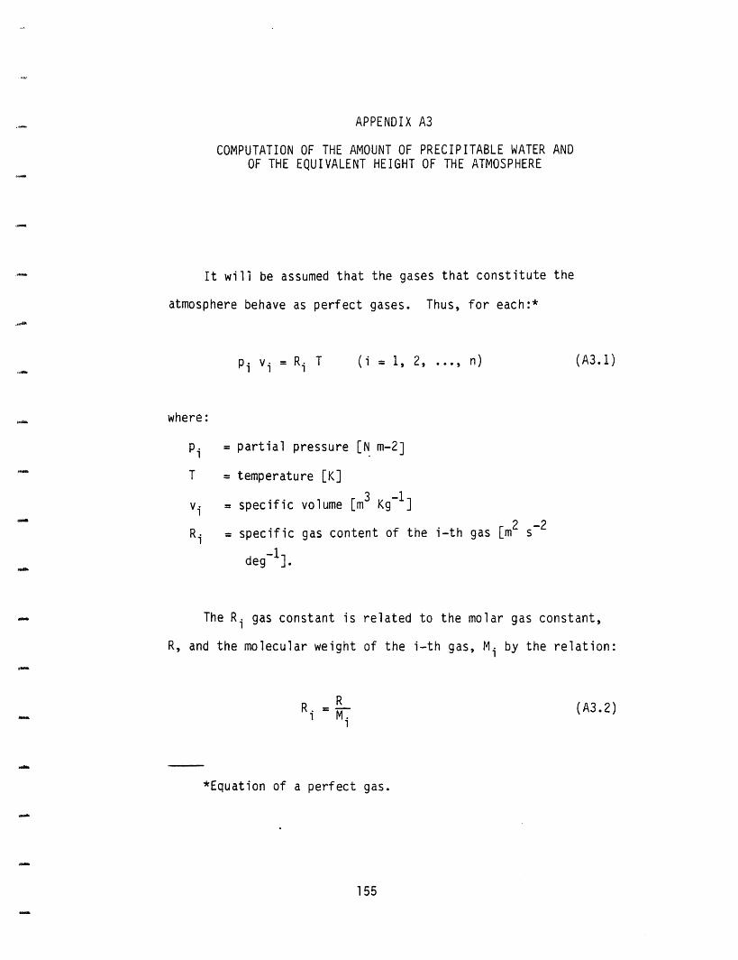
APPENDIX A3
COMPUTATION OF THE AMOUNT OF PRECIPITABLE WATER ANDOF THE EQUIVALENT HEIGHT OF THE ATMOSPHERE
It will be assumed that the gases that constitute the
atmosphere behave as perfect gases. Thus, for each:*
Pi Vi = Ri T (A3.1)
where:
Pi = partial pressure [N m-2]
T = temperature [K]
vi = specific volume [m3 Kg- 1]
Ri = specific gas content of the i-th gas [m2 s-2
deg-1].
The Ri gas constant is related to the molar gas constant,
R, and the molecular weight of the i-th gas, M i by the relation:
(A3.2)R RM.
I
*Equation of a perfect gas.
155
( i = , 2 2 . . . n )
lli
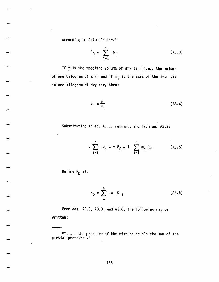
According to Dalton's Law:*
n
PD = Pi (A3i=1
If v is the specific volume of dry air (i.e., the volume
of one kilogram of air) and if mi is the mass of the i-th gas
in one kilogram of dry air, then:
Vv. = (A31 mi
Substituting in eq. A3.1, summing, and from eq. A3.3:
n I
vE Pi = v PD = T E mi Rii='l i=1
.3)
.4)
(A3.5)
Define RD as:
nRD = E m R i
i=l
(A3.6)
From eqs. A3.5, A3.3, and A3.6, the following may be
written:
*". .. the pressure of the mixture equals the sum of thepartial pressures."
156
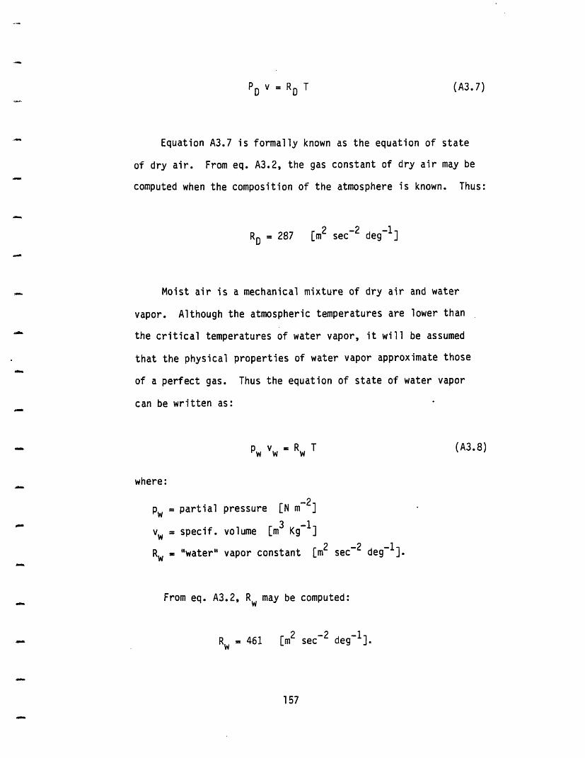
PD v = RD T (A3.7)
Equation A3.7 is formally known as the equation of state
of dry air. From eq. A3.2, the gas constant of dry air may be
computed when the composition of the atmosphere is known. Thus:
RD = 287 [m2 sec-2 deg- 1]
Moist air is a mechanical mixture of dry air and water
vapor. Although the atmospheric temperatures are lower than
the critical temperatures of water vapor, it will be assumed
that the physical properties of water vapor approximate those
of a perfect gas. Thus the equation of state of water vapor
can be written as:
Pw Vw = Rw T (A3.8)
where:
Pw = partial pressure [N m-2 ]
vw = specif. volume [m3 Kg-1]
Rw = "water" vapor constant [m2 sec-2 deg-1].
From eq. A3.2, Rw may be computed:
Rw = 461 [m2 sec-2 deg 1].
157
The dry air and the water vapor are uniformly distributed
within the entire volume, v, of the moist air; the specific
volumes of dry air, VD, and water vapor, vw, are:
vD = v/(1 - S) (A3.9)
V = V/a (A3.10)
where:
v = volume of kilograms of water and (1 - a) kilograms of
dry air.
The equation of state of the dry fraction of the moist air
may be written as:
(PM - Pw) VD = RD T (A3.11)
where:
PM = total pressure of moist air [N m 2]
Pw = partial pressure of water vapor [N m2].
From eq. A3.2, the following may be derived:
Rw/RD = 1.608 [adimensional] (A3.12)
By substituting eqs. A3.9, A3.10 and A3.12 into eqs. A3.8
and A3.11:
158
Pw = 1.608 R TPwaD(A3.13)
(A3.14)(PM - P) vl/(1 - a) = RD T
Adding eqs. A3.13 and A3.14 gives:
PM v = T RD (1 + 0.608 a) (A3.15)
Equation A3.15 is known as the equation of state of moist
air. It may be rewritten as:*
(A3.16)PM v = RM T
where:
RM = RD (1 + 0.608 a). (A3.17)
It should be stressed that RM is a function of the air
humidity, a.
*If the factor (1 + 608 ) is considered to affect thetemperature term, the concept of virtual temperature, T, isintroduced (T = T(1 + .608 a)) and the equation of the state ofmoist air may be written in terms of the dry air gasconstituent. This is often done in meteorological applications.
159
Defining the mixing ratio as the ratio of the mass of
water vapor per unit volume to the mass of dry air per unit
volume, its numerical value will equal the amount of water
vapor per unit mass of dry air.
From this definition and from equations A3.S and A3.11,
the relation between the mixing ratio, MR, and the air
humidity, a, may be simply derived:
MR - (A3.18)1-a
The difference between the mixing ratio and a is very
small.
Recalling eq. A3.11 (equation of state of the dry fraction
of moist air) and eq. A3.8 (equation of state of water vapor),
the mixing ratio may be expressed as follows:
MR = (RD/Rw)(Pw/(P - Pw)) (A3.19)
Therefore, the equation of state of moist air (eq. A3.17)
may be rewritten as:
160
RM = RD (1 + 0.608 MR)
1. Precipitable water computation
With all these concepts established, computation of the
amount of precipitable water may be attempted.
It will be assumed that dry-bulb temperature and pressure
are known. The amount of humidity will be considered through
the dew-point "temperature," although other parameters, such as
relative humidity, might be used.
The partial pressure of the water vapor in the gas mixture
may be computed, using the following numerical solution of the
Clausius-Clapeyron equation:*
logoP = 10.79586(1 - TSK/TDp) + 5.02808 log10(TSK/TDp) P) (A3.21)
+ 1.50474 10-4[1 - 10-8.29692(TDp/TsK - 1) ]
+ 0.42873 10-3[104' 76955(1 - TSK/TDp) - 1]
- 2.2195983
*From the Smithsonian Institution, Washington, D.C.
161
(A3.20)
where:
Pw = partial
TSK = 283.16
TDp = station
pressure of water vapor
[K]
dew-point "temperature"
Note that eq. A3.21 furnishes Pw in atmospheres; its
conversion into S.I. units will be implicitly assumed from now
on.
Recalling eq. A3.8, the water vapor density may be
computed as:
(A3.22)Pw = Pw/(Rw TDBK)
where:
PW
TDBK
= water vapor density [Kg m-3]
= station dry-bulb temperature [K].
Recalling the concept of "equivalent height of the
atmosphere," the amount of precipitable water may be computed
from the following relation:
w = w Hw w
where:
w = amount of precipitable water [mm]
(A3.23)
162
[atm]
[K].
Hw = "water vapor scale height" of the atmosphere [m]
Pw = water vapor density [Kg m-3].
A dimensional analysis will help to understand eq. A3.23.
Recalling that 1 kg of water = 1 liter of water = 1 dm3 of
water, the dimensional analysis of eq. A3.23 would be:
-3 -2 3-2 6 3 6 2[Kg m m3] = [Kg m -2 ] = [dm3m 2] = [106mm3 10mm-2] = mm
The "water vapor scale height" of the atmosphere (or the
equivalent height of the atmosphere generally adopted in those
applications) is two kilometers. Seasonally optimized values
for different "Standard Meteorological Areas" have previously
been computed.
Due to complete ignorance of the even low atmospheric
movements here assumed, the precision of this calculation is
low; final results may be obtained with an error range of 40
percent. The consequent error of the E0 computation may be
immediately derived from the sensitivity analysis plottages,
reported in Chapter 5.
The results of the amount of precipitable water
computation for a location at which temperatures, pressure, and
experimental precipitable water daily values are available,
follow:
163
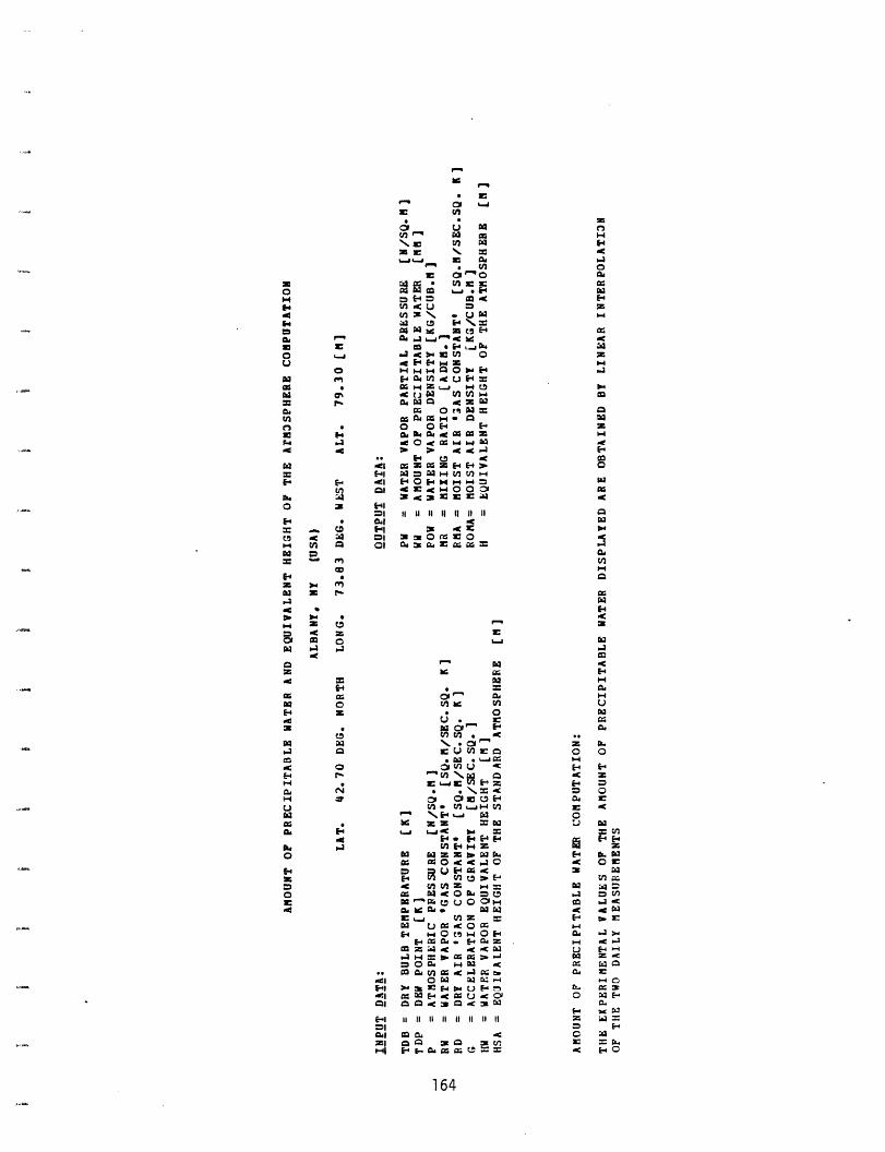
a1=
Yz C = -UI
v0 2
* OE * E-94 t1n Cffl 0
4 E1D IM W b as E-4
-4 W 6" W
V vI E"
* 1 , Z=
tl; , H 5Z -[ Ck W C UC-4 =ad M 4 Z
tn 9s1f a= H * ,e I 0 54 j...4o * o Eat-,U
554 54 = a H inM 4
Oc 1 E 1 Pl=Sa. E-1
CD ad1 1 bH-1 ne ;* 0 05 C 2S 4n o l lowSac M H
2 5
2 12i
54 > * 0
3 O
a wI C
M C
0' 0 0 L.N
4 43UVlra 4 a
E 54 4 * -Cv 2 a
54U 2X * 0 4 2 * Iot54 Z Z
U F l, v< W -= V- 0 I ) t P 54
e * EL~d 2 W4 ow Oa
n z = EIi r A
H c 0U OH ad 2 -bia~ 34. b U i 0- C
a t E = a -4 3a.I UG G2 rb IC M3
3 <1 M n3 E a. Ua 54 rn-a ra c a 2 a
l i 113 C 11 1 M.1 a8-1 or ,
01 ix no O-C - 01 :O 4E-200 54 I 4 a -E54 H0CA;O54 a *.-SJ)
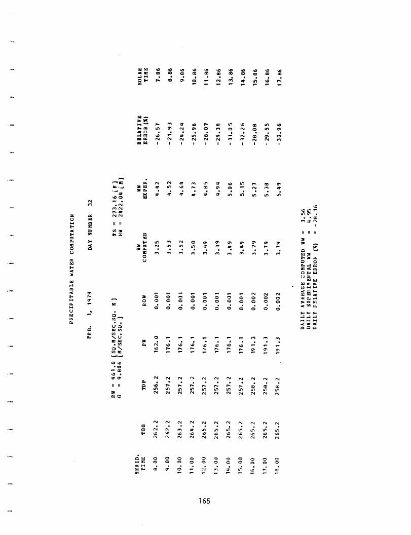
* W * o l* * * * . o
F= r, ~
°EP r~ m 0 0 _ N _ \ c 0 %C
o Ln 0 N 0% o 0 ~0o N 0 - 0) * * * * * * * * ./
a N N N NN N I I N a I I I I I
; t% N -t tn uli :r '. Ln P m oIno *r a O P co , C - N t
Wb4 * . * L. U. * . 'A.ad
II II
0
F~ LA t N 0 0% 0% 039 r4W) l M z gr ZsN LA
S S * . .3: e m t^ en A 4 0u
o 0 0 0o 0 0 0
o O O O
9- 9- -. -
p- 9- r- 9-N N N N
N NS N N
N N N N
'a 0 ' '!
o 0 0l 0
_J 06 6000J
N-
II It II
3I-3 *
0
fN 4 C
C O z OaO la O :- N CN N0 0 0 0
o 0 0 0
OA OA ...... O O L KN N N.. .N *
>4 4 :.
o . . 0
o o O C
O o O s. * .
S iC rv c_ _ .s
165
-
'00N ,-.
.4
C
E4
o
E-
UH
-_ 0
E3ol*C.
0
II II:
1 0o 0
a N0
I
0 N
40 '0
N
0C
o 0o 0
o o
N N
N N
o 00c C

C4 n LA LA LM LM Lm Lm Un t Un Le 0 G o 0 Go c CI co 0 c co4OI 4 . *
0 Ef 0 0 0 N e * uA 0 5%
~ '
0 _ _ ,,o N N -e 0 N - cc
^ . 0 0 . . * . . * *z 0M0* L Cl 4 04 _. L A_"'~ N e N N N N N0 1 I I I I I I I I I I !
e ( _ LA LA >0 , - r c ON9 4 a, 0 - N M 0 U %a 5% 0 0%
W in LA LA LA 'A LA 'A U LA LAM3
E
IU
LA L N 0 0 L N N LA LA % - - :r T 0T :t* . . * . . . . . * ;
^~~6~0 0 * 0 0 _a
a 0 0o 0 0
O0 0[XQ. N N
0 UoN NC4 N
N N0 N N
N N
- - No O 0
* 0o 0 0
- r a
LA LA LA
n _ %x%C Io xCN N N
o 0 0 0 00 0 0 0 0
N No oo 0* 8o o
* 9
o 0N N
N N
*n 0
eN N
N N
'~0 %Q(V 0Nv N
0 00 -,
* 0
N N0 0o 0
0 0
*.
LA LAut Nc N
N N
0 0N o
NN
r rN CC
qCI
0 00 n
A ;a- a-
CN N0 0o oo 0
N N
N N
*
N J
N Nt Cl t~x
0 0
r 0
:;H
X F
166
e O
n( ,0X 84
II IIw0
0z
z0
E-4
as
E-4
Ca'-402-C
H
U1404
0
I
aa i03
3 0
064Uz
000N
* 0hi 3
* iC
0\
o ,Lj LJ4
o':0
_ a
II II11
=; V
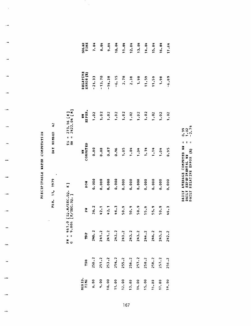
a * . * * * * * * * *
:.- -_ I_
0 m 0 co 0 c c C a U, O
F4 ; 0 n e n - 0 0 LA 0 0VS :Y | | |
_ S
- IC 1; N N N N N ( N N N N NW. J c a 0 0 0 0 CD 0 0 0 0S~ ~~ SMP -_ Is a, 0
:t 14 - -- - 9- : -. 9- -
'N 5:r *
0i N N
0
C-4 0 0 l* 'D Ln" * * * * _ L
r 0 0 0 0 - - - - _- 00
0 00 0
0
0 00 00 o
o o
0 0 0 0 0
0 0 0 0 00 0 0o 0o o o o o o * * *
*0' (N0%0* *N
O_ |
II II I
C~. 11 ~;:s~0 -
0 0C a -
:,t old=1.1.C
Oa Ei L) ZH h
000X S >
< ; P
W; X <
F XW
Ie Xcx
> >*
c1 H HWe <4 a
000
N; s~ 9- 4S 1 0% 0% a' 0% 0% i%
IL 0 CN N '.0 0 0 u0 Ln 0 '0rn *- _* * Ln Ui) LA L A LA) *l
N N
rAN N
N N
N N
0 00 0
0: 0
N N
* *N N
* U,
0 0
ot 0N NO OO O*N
N N N N NV
* * * * *N t N N N N
N4 N N (N N
%0 r W W 0LA tr LM tn U1N N N N N
0 0 0 0 O
0n 0 0 02 0* . A * . 15- - 9 _
(N
N10
CC0
167
II IIW
z1%.=a
-CQ0
(r
I
0HD,4
1-4
yk.W0
U
W3.CA0143
14
*cm-
H0UHu
0 or0
0
0IA-a _
* i t
..
o
*0
a 0
N
0 0E Or.4 *
N1
N
0 0
a N
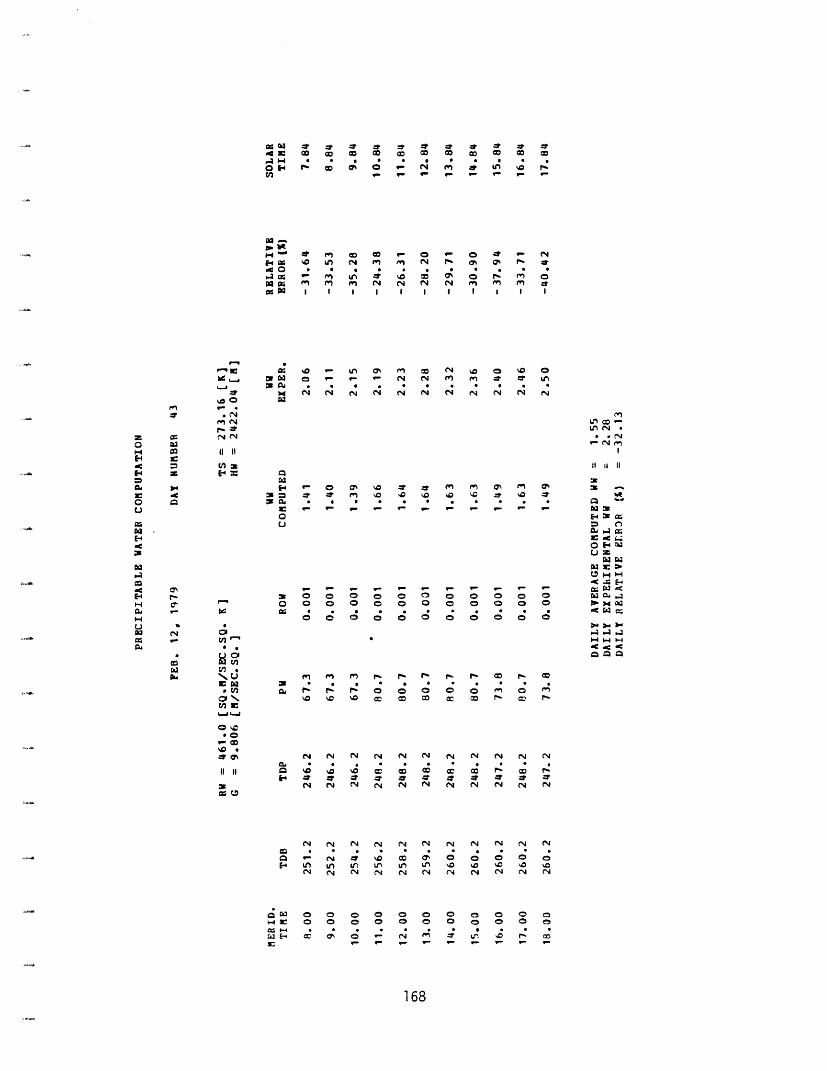
-r n L * ' LA0 t en o
=D _ .
iH _ : ~ e- o - o o . N
M I - M I N N !o I II I I I I I I I I I I
"c a: O L 0 C e = N '.o o 'C 0kg . :h 0 * .- ' N (N m m * * un
" c 4N
ICiia il 11
a3.0 ' 0 0% ID -* a Mn n Cy' e
:s = :s, 4t m la 1o o Q <c -I %QD * * * * . *C . .C * '0
0u
. 0 0 0*= = 0 0 0
0 0 0
~- a- -0 10a ;o 0 0 0 0 0
o 0 O 0 0 0
O OO OO 0 . * *
0 0 0 O
eN N
II i1 II
0%"
a-
4CU
a
-C g Hin Q
;2 . . . . a . 0 . a 00 %C r 4 0 0 co 0 c 0 ^ o en
'C \0 'C C: C1 0DQ 5 S C
N N N
a4 * *
N N No
O N *= 0 0 0O: h _ O O OJ00o
N N N N N N N
N N N N N N4 N
O O 0 O 0 0
168
N
tz
N
N
00:
0
z0Hj-4-C3.4
0DaUhi
Ca3.4
Uthr04
asr-LI
N
*
co N,
: Ca3 LA.
ra
UM oCA0 '.o_ 0%
II II
2
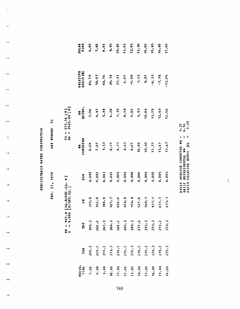
L in in L t tm LAn L t km tn LA< 0 0 0 0 C 0 0 0 0 0 0
C 0'-D .-
cGI 0 rl O - N 0 0 - o r P 0%a; rr rr
C P 0 0 N o r L 0 O
W m L 0o P; 0 0 0 - N s0 - - -
%~ N0C* *0C C D
r - -= -1-4 4, P. P. '- - LA LA -I LA - P. P.W L 0 ) LA - . Q O 0 = r. %O XS C * . . c * . . * . 0 .
o - - - - -0
f" en= 0 0
0- 0 0 0
0 0
o 0 0 0o 0 0 0
0 C 0 0
o 0o Oo 0
0 0
C .
Ut .-I.1
N N
N N
4' 0N N
o Oo o
_. N
o oO 0
o 0
: 0
4' P.LA N
NN
'0 P.
rv r-N N
'0 '0N N
o 0o oo 0
P1 4
Or n LA Ln
o 0 o 0O O O . * *
O O O
II II II
iW0 0
E 3 t40 0
0 .4..
r4 3 :.H I-4 H
0W0b.. .. .1.4 4 .H H .c 4 -CZ in C
G- - _9 _0 1- _- _UZcc Ln :; - 9-
NJ N 4 N
N N N CS N
L 4' LA Ln
O 0 0 0U; l 9 C
169
L-
O 0
N _ x *N
rv :tC
II II
n 3=E-.1=
zOHI,4
O
U.3
HL)CHU0
0aCa
3
bZ
N
011Wu
er
l 0* .
rn
. 0
01
O r
-'D
II II
o 00 023Cdw 0 N
P1
N e
atn xQ9 %Q \o
C4dP LA vo5-4 R
o oo 0* 14o 0
G~ 10 .
% N0 46x :t
N N
*. 0iOIN N
N N
(1V
N fN
NN
N N
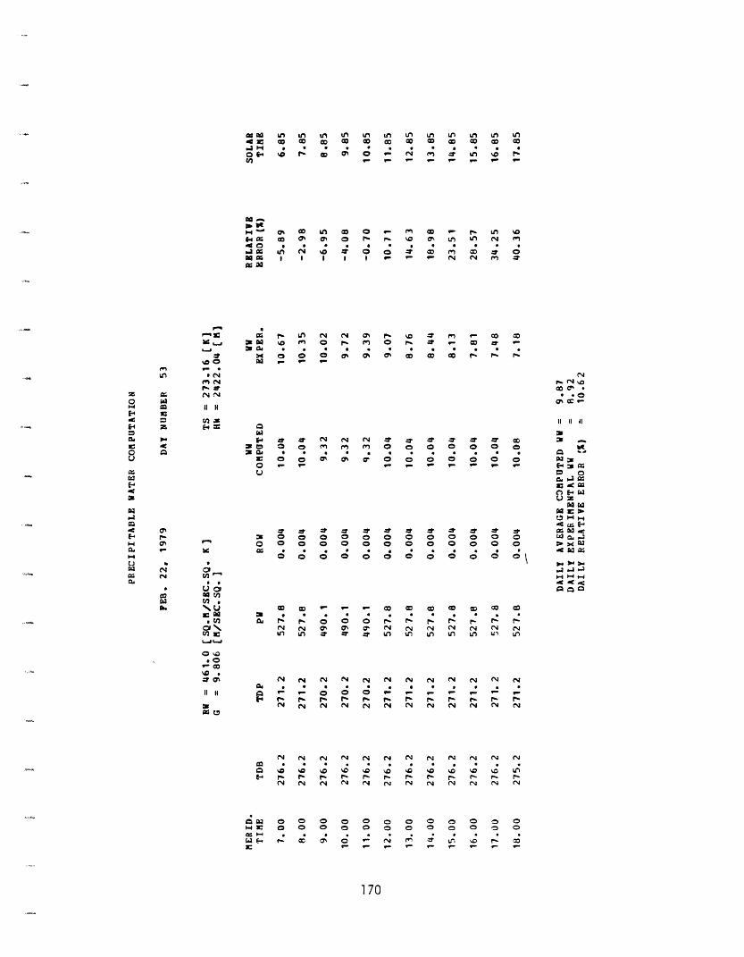
M uL LM LA LM tn LA Ln Ln Ln tn Ln LA
r ·
.41H * * . . * t * . OO4 c@ r 0 o% 0 _ N M LA O f
AJ LA N * * 0 * 0 f co * 0lO GI I I N N ,n =; Ad
O; '. O N N a F~ 'D - - 0 me 04 % en 0 r' a r. - _ 0 *r -: *33 w
H o 0 0 0; 0 0 0 0 9 - _ _
* .0% a:_
0
P _r : N N N _ -t _* * AT :x I 0 0) en M M 0 O 0 0 0 0 0:s 12 0 =O * . . *.
E 0 0 0 0% ; 0 0 0 0 0 0 oo - - 9- - - - -
U
_ _ -0 N 0 0 0 0o 0 0 0 0O * * .S
o a 0 0
0i co o -
in LA z a*
04 * * S
0 ' - 0 0
o Sr
N N N N
H=r
EUJt -
o0 0 0 0 C C0O O °
* * * -~ G o
o 0o 0
o 0
o rt
-. L
N N
o N N
o 0o 0
0 0
I- rN N
Ln LA
N N
- ·rN N
N N
N N
o Oo o
* N_ N
O 0(= O
el r
o oo o
o o
It -o 0o o
II II II
0
U z11 9
H H H= a P o
4 14
in I= O
0 0
N NLA LAUZ UZ
N N
- 9-
N N
N N
N N
0 00 0
u ', .
C- , r
·N NN N
0 0r
0 0
toQ
170
r-k E
; NNO3 _ .z; *Nr-m I11,Ua 0
Z E 0E44
z2
,C-4
U
E
0
I.coHC.HmU
Ca
0r-
N
* SbN
g v,
.
* 0
-* 0
3
2. Equivalent height computation
The equivalent height of the atmosphere has been given in
Chapter 2. There it was shown how it is possible, for a
location at a zero elevation, to avoid its computation for the
determination of the density integral, A.
However, H may be computed as follows.
i. the mixing ratio is computed from eq. A3.19;
ii. the moist air constant is computed from eq. A3.20;
iii. the moist air density computation may now be performedfrom eq. A3.15 (the equation of state of moist air).
Therefore, H may be computed from eq. 4.7:
H\= P(O)/[p(O) g)
where:
H = equivalent height of the atmosphere [m]
P(O) = sea-level atmospheric pressure [N m-2]
p(O) = moist air sea-level density [Kg m-3]
g = acceleration of gravity [m s-2].
The results of the equivalent height computation, for a
location at which temperatures and pressures are known, are:
171
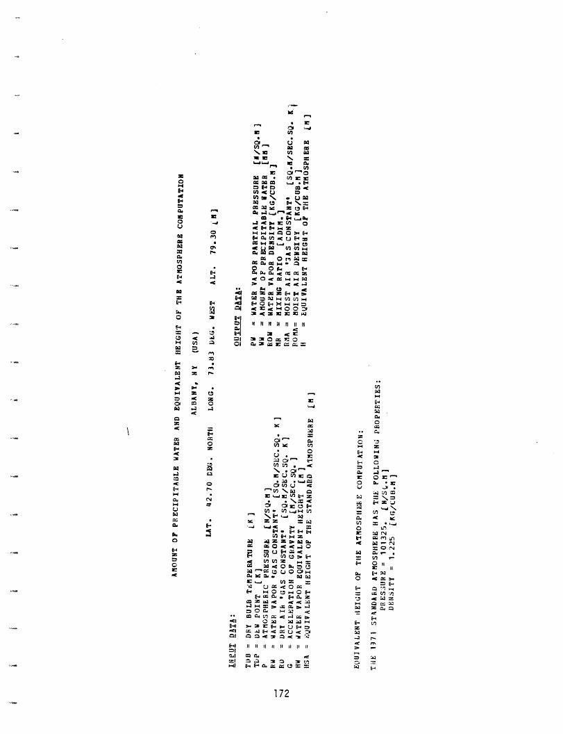
WJ,da u
a u
VI w a a;
z~r a; a zO
I Q; 14 .
IC to epo w 4 <F L n o
Q 04~~~~~~~U o E ~mb W =
E-4 ~'"
.-E-4 H 9 a O > =uCD r 3 1 < : a3 ·L. a U: f- ,
Vt CC °·o * o o P~CO im 0 :
1.4~~~~~~~~~~~~~~~~~~~~a<: ¢ > pb < <G~
W 0b g~nE- 4 05 Z E, 2 - ",,C (0 . M3O: s aa a OI ̂uz a
2c~~~~~- ~4 Cy r -4 E7 D~ -aN~~~ ' ~ x: ~' s =r Z 44 v·· Pc U 0IPO :s Ei Z~~
t, ~~~~~acNE- H
AQ r..C9 41
D.~ tl I II I tl II I II . .
· ~,-I 11~ " 1 .'~ 11 11 ,~ 113 ·i 3 1 a s OU w H V1 1 01 C S ; s: ; _
&4 C6Cn 0aZ 2 E
0 .
X~~~~~~~~E 0 0E J 'r.
a2~~~a~~~~~~~~~~ L _-G
E~~~~~~~~~~~~~~~~~~~~~~~~~-Vz;C; C '3a O U:X V c Z
eO U U 3 si t-( o~~~~~~~~~Zi :M :EF E a. = = E-l 72 O _ U=4 _ dlco 5 :4 V Z tQ v: -L~ Cn t_4z l va; * s ~nZ Z =*.
cc 3 UX r 4 Zt c z n -
o ;4 ZZ z 4 *e X-
z1 ti UZ UU O 2° =5 CcsY~ ¢ Zs 2:bo
a~~~~P WU al: ¢ O E: P
V)) Zz t~x - - <
a Y ~~m O U a :s: ^s -
ei V) 5: b 5:x <r
'1 UaOP 1O:c
z 0 Ir 4 a sz :r£ ss; 347; cn s
41 ~172
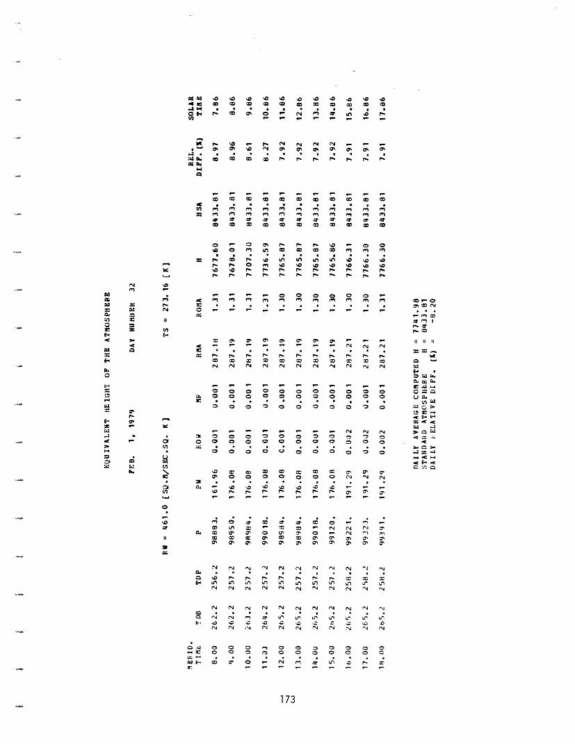
10 o 14 o 0 .0 w .0 laco c 0 0 - co 0 0 0
_ - - -
r .% _ f N N N N -. I la N 0% 0 0 ON a, 0 ON* * w * * * 5 9 . S *o 0 0D 0 r. tW P. S P.' f% r
9- - - - - - - - 9
0 0 0 0 0 0 0 0 0* . 0 9 0 9 9
t5.m Y~ 99~ m
= % ~ ~ , -,9t' ~f* * * ' * ' U
0 0 00 1~0 00
o 9- 0 r '." P." .0 9
2 0 f"r u 0 0 0 0 S 5 9 S S 9 9 0
= r.'.0 P' . U' U 4~ U
0az
- - - - 0 0 0 0 0
* . . I. . . .
- 9- 9- 9- 9- 9 - 9 70 0 9 0 9 0~
5r *. . P. *. . . *. p. .
= ~ j W>r
o 0 0 0 0 0 0 0 0 0'
o 0 0 0 0 0 0 0~0, O 0 0 0 0 0 3 0 0LC * * . 9 9 . .q0 0 0 :D 0) 0 0 0r
a - 9- 9- 9-9- v:-9 9 -
o 0 0 0 C. 0 0 0 0.0 0 ~ 0 0 0 0 r
0' 0 0 0 0
9- 0 .0 ~ .0 .0 4.0 p p P. p p 9- 9 9 - 9 - - 9 - 9 9 - 9
l 0 U 0* . . * 0 I.
N N N 4 N N N N N
Ei u un L) L V) - V)
N N ." CN N N N4 N N
o 0 0 Il 0 0 0 0 0 CD O 0 0 CD 0 0 0
0 0 0 1 9- N~ r 4
o 9m m 09-0* .ab
N N
30 0
0 0 =
0 0
3 3 ~4 C H~
0'0
0' ~ Cn
N C,
o'l J,
0 I: N
* N
Nu '. 1.Lr W
N N
O 0
o _* C
_: x
173
'-
049.3
i0 0
_ S99ro e
* CO
A 0
w *
0 0
o 0re r"
r .0 .I.' P.'
03 4m e2:m1§
IfI
0
I=w
rV)0sE-0
E-
0
H
0
Cf.
x
W911
H0
;a:
>
_ V)E-
_-Ca,0
QIo* Ua,
li0U' t6. '1
I,ooxit
C 1-04Xw :
L:
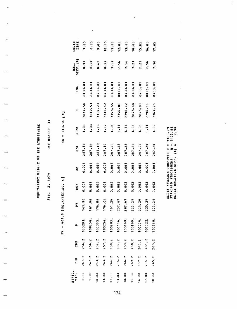
Qs W L Ln Ln LM Ln Ln Ln LM Ln Ln LA< C:o C Co 0a co 0- 0 M c co 0
M S 9 0 9 * 0 0 I * a
E ! 0 r i 0 Q r U - _ L o
. o I N LA LA L N f -A t
co 0 0 0 0 CD co c l r co
cc en n M en t
0 0 0 0N 0 0 0 0 0 0 0 n, I 0 oa O ' 0 co o 0 04
A LL 0 0 0 0 L N
n o. jJLA JJAjA. .90 ' N t- (O e 2
.0 0 ( 0 0 0 0 0 D 004 ~ * ' 9 9 N ' 4 ' -N
N. 0 * co * . , a * * 0 I 0N rn Io o N
E < - __ IC N N N N N N: : *- *m *r. m * * *- I
Ct ; t F t
-1 o o o o o o o o o oo or _
---- N N N N N N N a
0 N N 9 N N4 - a- _ N " I 0 0 o 0 0 0 0 0 0 0 0
N N N N N N N N N N N
' *0 '.0 '0Q 'D '0 . '0
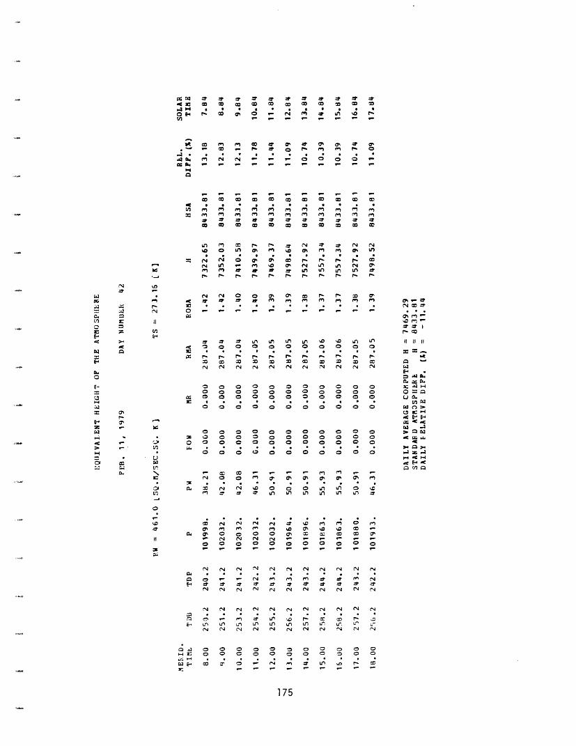
M co O o- Nc co
o * c *
s N 5- - - 0
-- - - - -
- 5 O D 5 co
N 0o 0 o rA _- o mo 09t, : * *
dD r p b O r
N 0 0 0% ON OU. . *. . .M M M_- _ _ _
. .N (N N tN N N
0 0 0 0 0 0
* * . ;0 0 0 0 0 0
N N4 0 0 O 0u. U u LA U LA
N N N N _4 _
5- 5- 5- 5i
- - _ -
Ln O) -
U. l_ N 4, 0% LA,r _
-0 l_ FLA A 0
LA LA LA U
_0 la Ln U If _. * I
1 O uj LA 111m 4%. 4 % Lh
E- 40 0
CZr?
Ln ~ ~ 3N N N N 4 .30 0 0 0 3
0 0 0 4,)z
LA LA 0 0 0
L* uL * *
4,) 0 4,a '0 0 33 0% ~~ro 0 0 0 c a az
U. . . U. >a
o o O 0 ZH CA P.C}Un
more_
. . * .
un n o wU: > S s
. . . .
r n o ,_,
3D x 3
_ _ _
o o °
r4 r
* . .
:t :F - C
Nr w C z
N C c ¢
L( . .t*
5NN
tn ,^. W N tS N o
Vs o o oo . o
175
0 14 T
.4 S4 a:.
L en
= ) co r:t
LA
=N
I-.
N T
z LI>4
:
W
0
:E-
04
E-r
0%-
T
ol
E-
u0.
:4
E-
C3C
N
U.0 -
-C49Mx: rW-
N
0a;OC
0
000
0
0%
0
W.I
U
3W
011MW
N
0 0113
.-.
NN
I.4
C~ O,4 o o- . L,; i a 0CYE 0
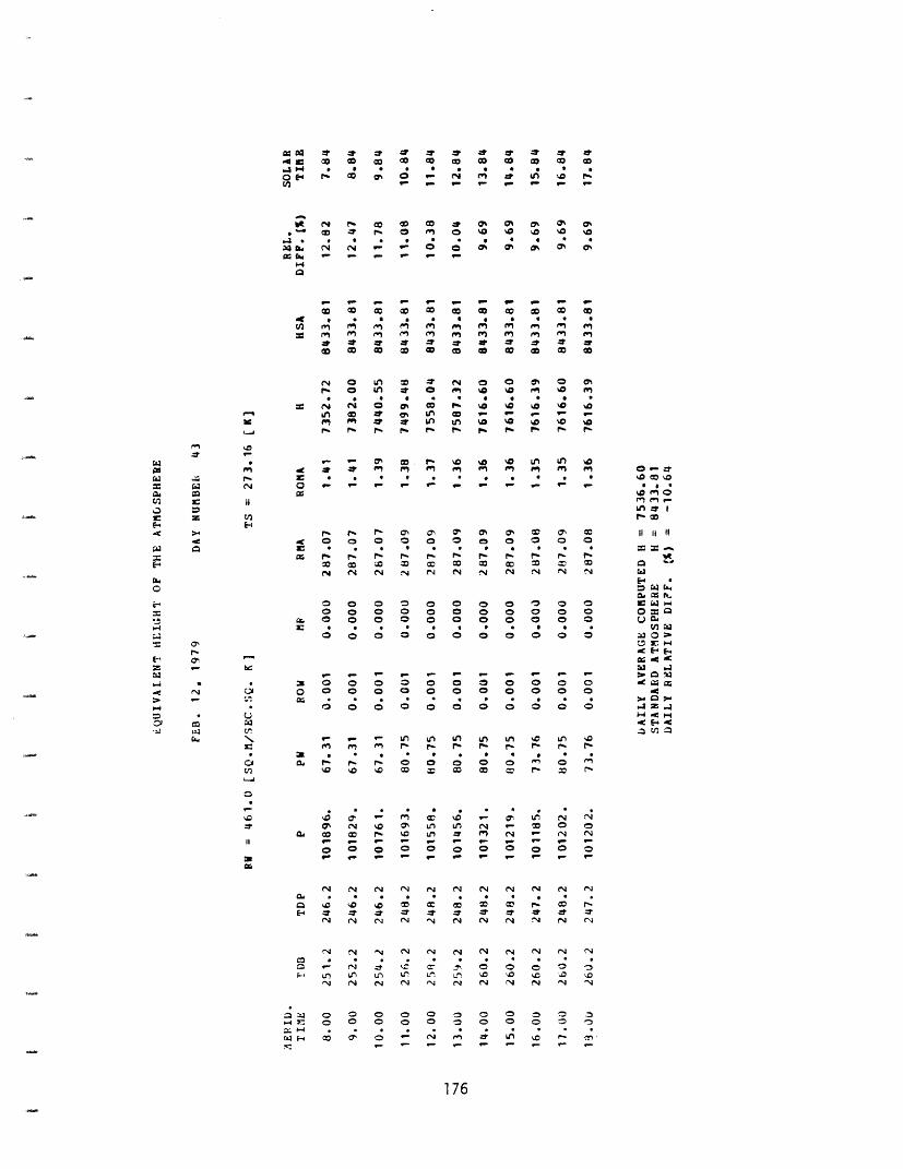
=p :~ =1 :~.X. * * *
; '- c; '~
N - 9- 0
0 0 0 0* * . *
0 0 0 0
o 0A 0
o JA * oO 0 0 0* * ¢
0 0 0
* * 9_ _3
C.. Ir- o
o 0 0 0
* 9 * 0qb
_ - _- _
* .
~. r- 0 0
0 J : Izaaj
J J J
9- t-) G
'0 '0 0 0* * *N · N N
j- 9- 9-Q?~~z
It cr cr _l c
* * * .0 0 0 0 0a_ A ; 9_ _ -
*a40
*0rco.
0% 0% 0% 0% 0%%0 '.0 '0 '. '.
a 0 0 0 o 0 0%
_- - - - -
M M M On M
4r at gr _- w
co co O do Me0 0 a 0~ 09-, i9 (9 49 It,0* * * * *
r* 0a %0 WD W
0D _- - _ 9-LA '0 '0 '. '.0r. P* f P. P.
'. %a wo U. U.
_- - 9- - 9
- * - . * e.-
NS N N N N
* J0DO o o O o
un n n u
r rv F
* * * . *
o O o < o
co c b3
'.0 _ 0, ut NLA N ,- 0 0
0 0 0 0 0
9- - 9.- 9- 7N N N N
* * * * *
N N tN N N
NS N N N N
* LA ' . 4'.3
_- - 9- _- 9
176
049
MM
coMaaI9,
'0
'0P.~
oU-*M 2-Irr
'.;49-00 V0* 0-
E-eP.OZO 0 8=
O UN* UCa5o O
o¢* CA o >
o 4z4-
d ¢ Ht< Es
n U:
0N
0
N
10'No
O E rl0~ ~o
a3 · N-I
m N
r4
= r
c o
ic 119-
ix : e0 ( 0 -ix
-CC3r P.M eE
0Ca
0a(11
ICE.
0
0'IV,z
00
M 0a:
0o%
N
(4
'a.cw~
0 Oo 0
at *
%a000 .
'O
0%Jc0V-
11
crU
:N,
31'9C'
0'0
I,
0
= 0 0f4H 0W F-. :7cr
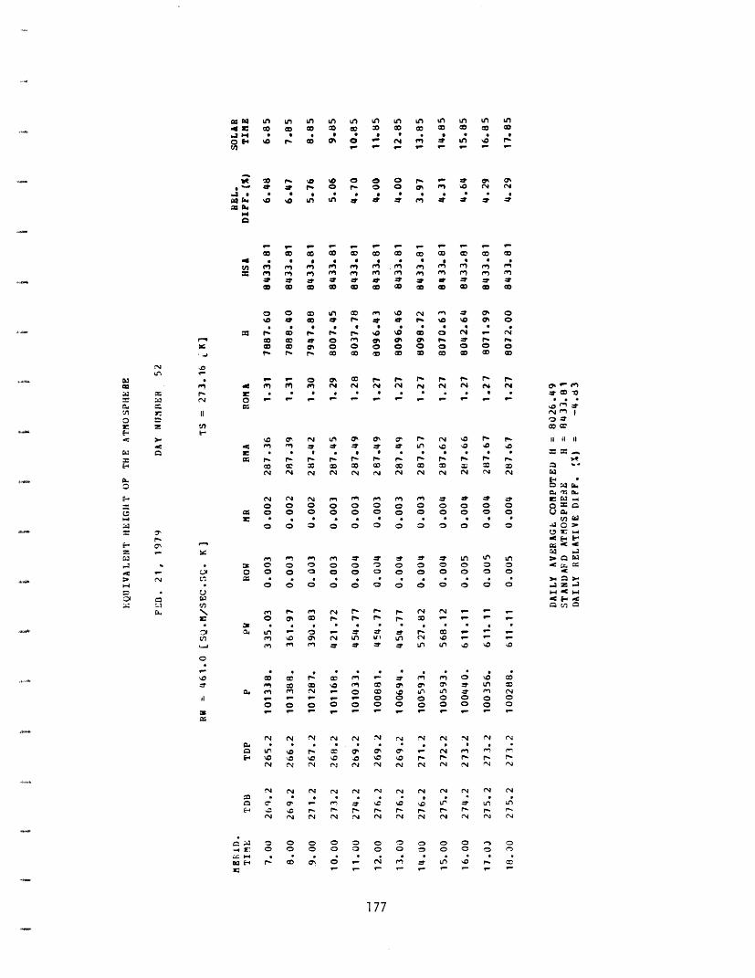
, U, n un u, L ut
*0 a 0 0 * .0
9- - ,-
Un un un un Un
0 0 0 0 9- 9- 9- 9-
0 % 0 0 0 0 - - r 0 0%2t * t 0 O 0 0 O fn 10 N N
e 9 0 * 0 0 'a n in * * * * * * * _s0 o Z $ :e :E t Ut : :
0 0 C 0 0 0
, 4 m 0 r 0n=1 _1r _s' _1' x e :3'0 CD W 0 c a D
o CO CD c coW 9 W 0 *0 t0 00 '
C., mn
* * U. * 0 0 000
o a a) u, 0 f1e % N e r Cy 00 * * U. * * -* 0 la 0 0
go 0 r-r 0 e 0 10 0 0 N _ N0
0 0 ' 0 0 0 0 0 rC 0 0 0
o01%
- - 0 C W . r I- r- f- r- tfn rn m N N N N N N N N N
.: . -. . . . . . . ._- _ _-_ 9_ 9_ 9_ 9_9_9_9_9 _
0% - n
*r W -
c0 .o I00C:
0 a, N u 0 0 N 1 ( 0 ' " 11 It II
.t . . . . * . . 1. . . . s _
cNNN
o C 0 o 0 0 o 0 o 0 0 00 o o 0 o 0 0 o 0 o o 0 o
r * * .* . ' * E
00 0 0 0 0 0 0 g0 0n 0 0M 1
o 0 0 0 0 0 0 0 0 0 0* . , . . * . . . . . * 0 0
C E 0
C') 10 0 N U, I U N o - -z ; N In U. * *, *f *0 . *
0 MI 0 T _ L m 0 0 0-
o o 0 0 o 0 0 o 0 0 o o
N N N N N
E 1 1 0 1 0 1 0 .0
In C, *7 * * -
C ' 10 --N N NS N N
-4 1,= ;4
a H
E F
0C) 0 00 0 0 0 0:4 C % 0 9-* @ *
br
0% e ·N
10 0 ~ Cl N N N J N N N N
~ J JC\I
177
4 :
= w
r-CIa
6
Le
CW tC43 11
In
WEc
tmtC-T.0
E--
u0
0
HC:I
-
N
ICL.
C;
UI
Ul
W.0;
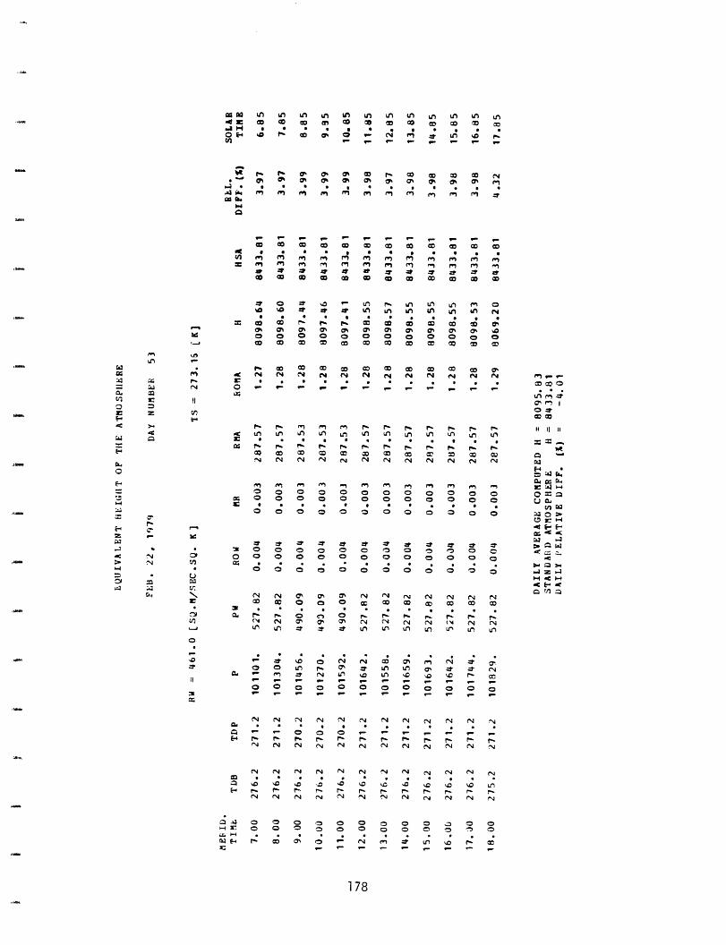
W W Ln Ln Ul LA in LA Ln Ln LA LA LA Ln
CiO X N 0% c P c O o CO NC0 0% 0 0% 0% 0 0 0 0 0% 0% 0
VW n In e M In
:. j 0 0 0 0 0 0 0 0 0 0 0 0 .
M a, M=) ( O N O0 0 0 0 0 0 0 0 0 0 0 0
OD o 0 o 0 o o co C 0 o
Y O o o O o o o o o o o OM; ^ < A N Nq N N N4 N N N N N N N
_ .a.J N OU-U-U-U- U-U-U .; V 2 ; ) rj _
E 4
E a*= Un Un . . In e n . M e .
N N N N N NN N N N N NrJW~~~~~~~~~~~ EL 3 cb~~~~~~~~~~~~~~~~~E-4
o 0 0 0N 0 0 04 0 0o o 0 o o 0 0 0 o 0 = 3 w: * . . . * . * * . . * 0
_ CE-
r 0 0 0 0 0 0 0 0 0 0 0 0* fN U 0 .C * * * . * * * * > . * .. . .
* 0 0 o 0oo 0 0 0 0 0 IZ* 1)H ¢ 1
A N 3 "4 N 0% 0% N r N N N N
* 0 0 LA* * . * * LA LA .% . * N
wU o o - U-} p. U- p. p. p
I '0 '0 '0 '0 '0 '0 '0 'n 3 '0 D LA
APPENDIX A4
INSOLATION CLIMATOLOGY DATA ON SOLMET FORMAT
Pages 1 to 7 of the data and format description of SOLMET
tapes, from SOLMET Vol. 1: User's Manual [61], are reported
below.
179
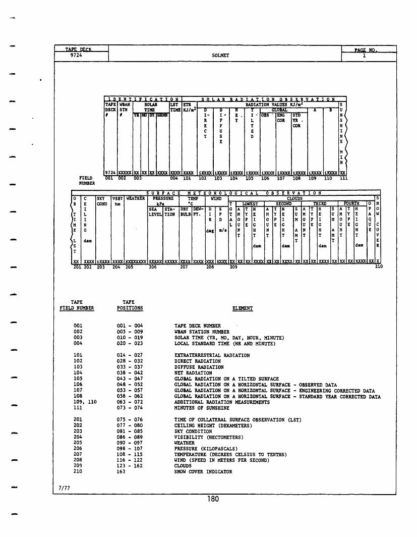
972TAPE DK PAGE NO9724 SOLMET 1
FIELDNUMBER
I D E N T I F I C A T I O N SO L AR R AD IA T IO N O BS RV AT IO NTAPE WBAN SOLAR LST ETR RADIATION VALUES KJ/m
2S
DECK STN TIME TIME J/" D N ' T GLOBAL B AUM I DY I" I, E . I 'OBS ' ENG STD N
R F T L COR YR SE F T COR HC U E IT S D N
E IE
N97 XXXX XXX X
97 24 XOOX XX XX X ]X X X XXX 10i0 1 10 10 05 D106 107 108 109 110 111001 002 03 004 101 102 103 104 105 106 107 108 109 110 111
S U R F A C E M E T E O R O L O G I C A L O B S E R V A T I N0 C SKY VSBY WEATHER PRESSURE TMP . WIND CLOUDS sBIE COND hm kPa *C T LOWEST SECOND THIRD I FOURTH 0 N
I SEA ISTA- DRY DEW- D S O A H A T H S A T H S A T H P 0T L LEVEL|TION BULB|PT. I P T M Y E M Y E U M Y E U M Y E A WI I R D A O P I 0 P I M 0 P I M 0 P I QMN L U E G . U E G U E G U CE G dg mn/s N H N H A N H A N H E O
T T I T M T T MT T VL dam T T ES dam da I dam dam R
x x 1 xxxx ixxxxxx xx x xxXuXXl I xx lx x x xxx l xxxlxx clCxx l CC xxxxlxx lx xxxlx xxx lx x201 202 203 204 205 206 207 208 209
ELEMENT
TAPE DECK NUMBERWBAN STATION NUMBERSOLAR TIME (YR, MO, DAY, HOUR, MINUTE)LOCAL STANDARD TIME (HR AND MINUTE)
EXTRATERRESTRIAL RADIATIONDIRECT RADIATIONDIFFUSE RADIATIONNET RADIATIONGLOBAL RADIATION ON A TILTED SURFACEGLOBAL RADIATION ON A HORIZONTAL SURFACEGLOBAL RADIATION ON A HORIZONTAL SURFACEGLOBAL RADIATION ON A HORIZONTAL SURFACEADDITIONAL RADIATION MEASUREMENTSMINUTES OF SUNSHINE
- OBSERVED DATA- ENGINEERING CORRECTED DATA- STANDARD YEAR CORRECTED DATA
TIME OF COLLATERAL SURFACE OBSERVATION (LST)CEILING HEIGHT (DEKAMETERS)SKY CONDITIONVISIBILITY (HECTOMETERS)WEATHERPRESSURE (KILOPASCALS)TEMPERATURE (DEGREES CELSIUS TO TENTHS)WIND (SPEED IN METERS PER SECOND)CLOUDSSNOW COVER INDICATOR
TAPEPOSITIONS
TAPEFIELD NUMBER
001002003004
101102103104105106107108109, 110111
201202203204205206207208209210
001 - 004005 - 009010 - 019020 - 023
024 - 027028 - 032033 - 037038 - 042043 - 047048 - 052053 - 057058 - 062063 - 072073 - 074
075 - 076077 - 080081 - 085086 - 089090 - 097098 - 107108 - 115116 - 122123 - 162163
7/77
180
I
Z10
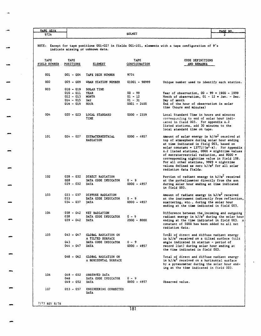
9724 SOLMET 2
NOTE: Except for tape positions 001-027 in fields 001-101, elements with a tape configuration of 9'sindicate missing or unknown data.
TAPEFIELD NUMBER
TAPEPOSITIONS ELEMENT
001 001 - 004 TAPE DECK NUMBER
002 005 - 009 WBAN STATION NUMBER
TAPECONFIGURATION
CODE DEFINITIONSAND REMARKS
9724
01001 - 98999 Unique number used to identify each station.
003 010 - 019 SOLAR TIME010 - 011 YEAR012 - 013 MONTH014 - 015 DAY016 - 019 HOUR
004 020 - 023 LOCAL STANDARDTIME
101 024 - 027 EXTRATERRESTRIALRADIATION
102 028 - 032 DIRECT RADIATION028 DATA CODE INDICATOR029 - 032 DATA
103 033 - 037 DIFFUSE RADIATION033 DATA CODE INDICATOR034 - 037 DATA
104 038 - 042 NET RADIATION038 DATA CODE INDICATOR039 - 042 DATA
105 043 - 047 GLOBAL RADIATION ONA TILTED SURFACE
043 DATA CODE INDICATOR044 - 047 DATA
00 - 9901 - 1201 - 310001 - 2400
0000 - 2359
0000 - 4957
0 - 90000 - 4957
0 - 90000 - 4957
0 - 92000 - 8000
0 - 90000 - 4957
048 - 062 GLOBAL RADIATION ONA HORIZONTAL SURFACE
106 048 - 052 OBSERVED DATA048 DATA CODE INDICATOR049 - 052 DATA
0- 90000 - 4957
Year of observation, 00 - 99 = 1900 - 1999Month of observation, 01 - 12 - Jan. - Dec.Day of monthEnd of the hour of observation in solartime (hours and minutes)
Local Standard Time in hours and minutescorrespinJing to end of solar hour indi-cated in field 003. For Appendix A.2listed stations, add 30 minutes to thelocal standard time on tape.
Amount of solar energy in kJ/m 2 received attop of atmosphere during solar hour endingat time indicated in field 003, based onsolar constant 1377J/(m 2.s). For AppendixA.2 listed stations, 0000 - nighttime valuesof extraterrestrial radiation, and 8000 -corresponding nighttime value in Field 108.For all other stations, 9999 - nighttimevalues defined as zero kJ/m2 for all solarradiation data fields.
Portion of radiant energy in kJ/m2 received
at the pyrheliometer directly from the sunduring solar hour ending at time indicatedin field 003.
Amount of radiant energy in kJ/m2 receivedat the instrument indirectly from reflection,scattering, etc., during the solar hourending at the time indicated in field 003.
Difference between the2 incoming and outgoingradiant energy in kJ/m during the solar hourending at the time indicated in field 003. Aconstant of 5000 has been added to all netradiation data.
Total o direct and diffuse radiant energyin kJ/m received on a tilted surface (tiltangle indicated in station - period ofrecord list) during solar hour ending atthe time indicated in field 003.
Total o direct and diffuse radiant energyin kJ/m received on a horizontal surfaceby a pyranometer during the solar hour end-ing at the time indicated in field 003.
Observed value.
107 053 - 057 ENGINEERING CORRECTEDDATA
7/77 REV 8/78
181
n
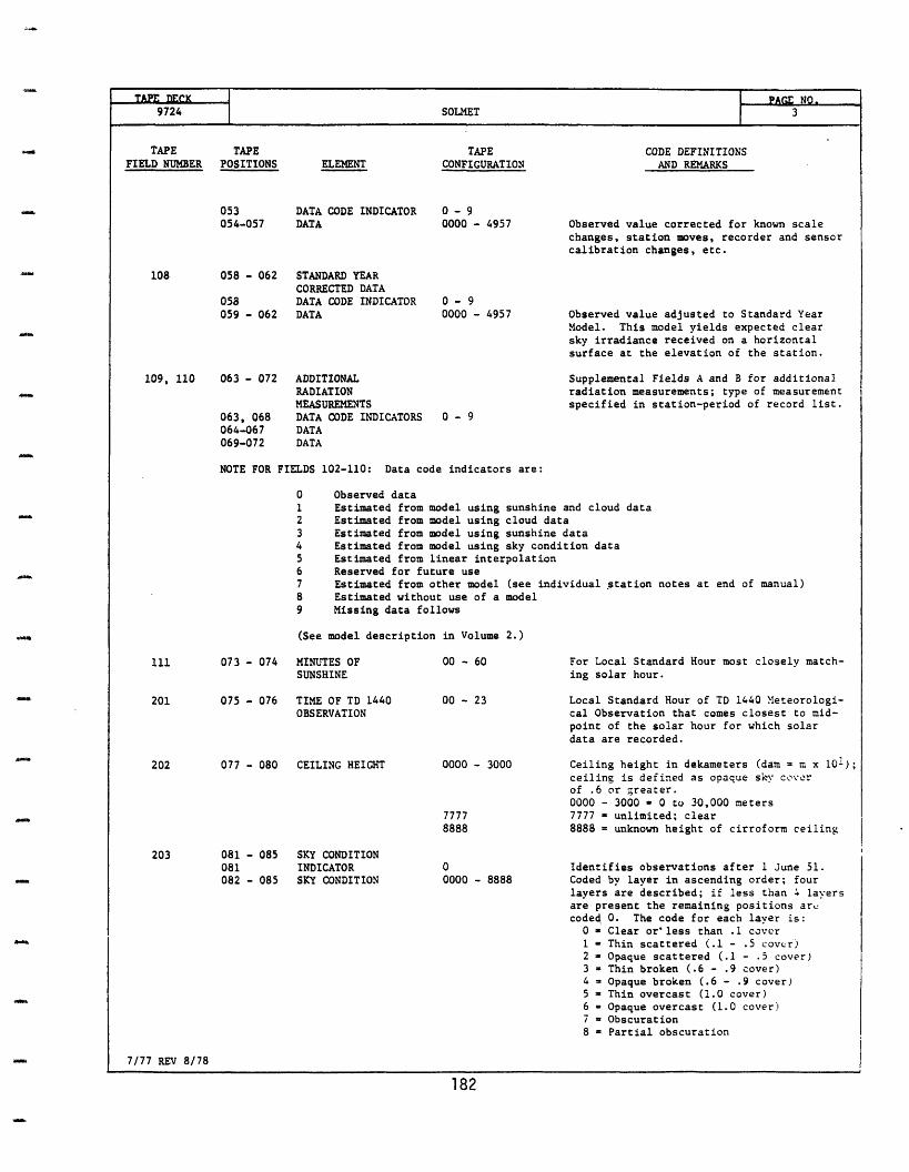
TPE ECKPAL NO.9724 SOLMET 3
TAPECONFIGURATION
CODE DEFINITIONSAND REMARKS
053 DATA CODE INDICATOR054-057 DATA
108 058 - 062 STANDARD YEARCORRECTED DATA
058 DATA CODE INDICATOR059 - 062 DATA
109, 110 063 - 072 ADDITIONALRADIATIONMEASUREMENTS
063, 068 DATA CODE INDICATORS064-067 DATA069-072 DATA
0 - 90000 - 4957
0 - 90000 - 4957
0 - 9
Observed value corrected for known scalechanges, station moves, recorder and sensorcalibration changes, etc.
Observed value adjusted to Standard YearModel. This model yields expected clearsky irradiance received on a horizontalsurface at the elevation of the station.
Supplemental Fields A and B for additionalradiation measurements; type of measurementspecified in station-period of record list.
NOTE FOR FIELDS 102-110: Data code indicators are:
0 Observed data1 Estimated from model using sunshine and cloud data2 Estimated from model using cloud data3 Estimated from model using sunshine data4 Estimated from model using sky condition data5 Estimated from linear interpolation6 Reserved for future use7 Estimated from other model (see individual station notes at end of manual)8 Estimated without use of a model9 Missing data follows
(See model description in Volume 2.)
111 073 - 074 MINUTES OFSUNSHINE
201 075 - 076 TIME OF TD 1440OBSERVATION
202 077 - 080 CEILING HEIGHT
00 - 60
00 - 23
0000 - 3000
77778888
For Local Standard Hour most closely match-ing solar hour.
Local Standard Hour of TD 1440 Meteorologi-cal Observation that comes closest to mid-point of the solar hour for which solardata are recorded.
Ceiling height in dekameters (dam = m x 10:);ceiling is defined as opaque sky cverof .6 or greater.0000 - 3000 0 to 30,000 meters7777 = unlimited; clear8888 = unknown height of cirroform ceiling
203 081 - 085081082 - 085
SKY CONDITIONINDICATORSKY CONDITION
00000 - 8888
Identifies observations after 1 June 51.Coded by layer in ascending order; fourlayers are described; if less than 4 layersare present the remaining positions arccoded 0. The code for each layer is:0 - Clear or'less than .1 cover1 = Thin scattered (.1 - .5 cover)2 = Opaque scattered (.1 - .5 cover)3 = Thin broken (.6 - .9 cover)4 - Opaque broken (.6 - .9 cover)5 = Thin overcast (1.0 cover)6 = Opaque overcast (1.0 cover)7 = Obscuration8 = Partial obscuration
7/77 REV 8/78
182
TAPEFIELD NUMBER
TAPEPOSITIONS ELEMENT
_Zp
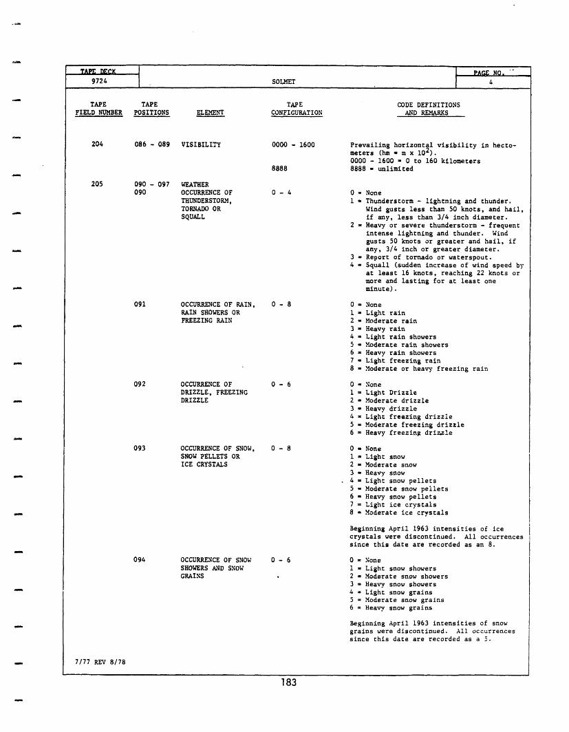
TAE DEC PAG NOSOLMET9724 SOLMET 4
TAPECONFIGURATION
CODE DEFINITIONSAND REMARKS
204 086 - 089 VISIBILITY 0000 - 1600
8888
205 090 - 097 WEATHER090 OCCURRENCE OF
THUNDERSTORM,TORNADO ORSQUALL
0-4
Prevailing horizontal visibility in hecto-meters (hm = m x 102).0000 - 1600 = 0 to 160 kilometers8888 - unlimited
0 = None1 - Thunderstorm - lightning and thunder.
Wind gusts less than 50 knots, and hail,if any, less than 3/4 inch diameter.
2 - Heavy or severe thunderstorm - frequentintense lightning and thunder. Windgusts 50 knots or greater and hail, ifany, 3/4 inch or greater diameter.
3 Report of tornado or waterspout.4 - Squall (sudden increase of wind speed by
at least 16 knots, reaching 22 knots ormore and lasting for at least oneminute).
091 OCCURRENCE OF RAIN,RAIN SHOWERS ORFREEZING RAIN
092 OCCURRENCE OFDRIZZLE, FREEZINGDRIZZLE
093 OCCURRENCE OF SNOW,SNOW PELLETS ORICE CRYSTALS
094 OCCURRENCE OF SNOWSHOWERS AND SNOWGRAINS
0-8
0-6
0 = None1 - Light rain2 - Moderate rain3 = Heavy rain4 = Light rain showers5 = Moderate rain showers6 = Heavy rain showers7 = Light freezing rain8 - Moderate or heavy freezing rain
0 - None1 - Light Drizzle2 - Moderate drizzle3 - Heavy drizzle4 = Light freezing drizzle5 - Moderate freezing drizzle6 - Heavy freezing drizzle
0 = None1 = Light snow2 = Moderate snow3 a Heavy snow4 = Light snow pellets5 - Moderate snow pellets6 = Heavy snow pellets7 = Light ice crystals8 = Moderate ice crystals
Beginning April 1963 intensities of icecrystals were discontinued. All occurrencessince this date are recorded as an 8.
0-8
0-6 0 = None1 - Light snow showers2 - Moderate snow showers3 = Heavy snow showers4 - Light snow grains5 = Moderate snow grains6 = Heavy snow grains
Beginning April 1963 intensities of snowgrains were discontinued. All occurrencessince this date are recorded as a 5.
7/77 REV 8/78
183
TAPEFIELD NUMBER
TAPEPOSITIONS ELEMENT
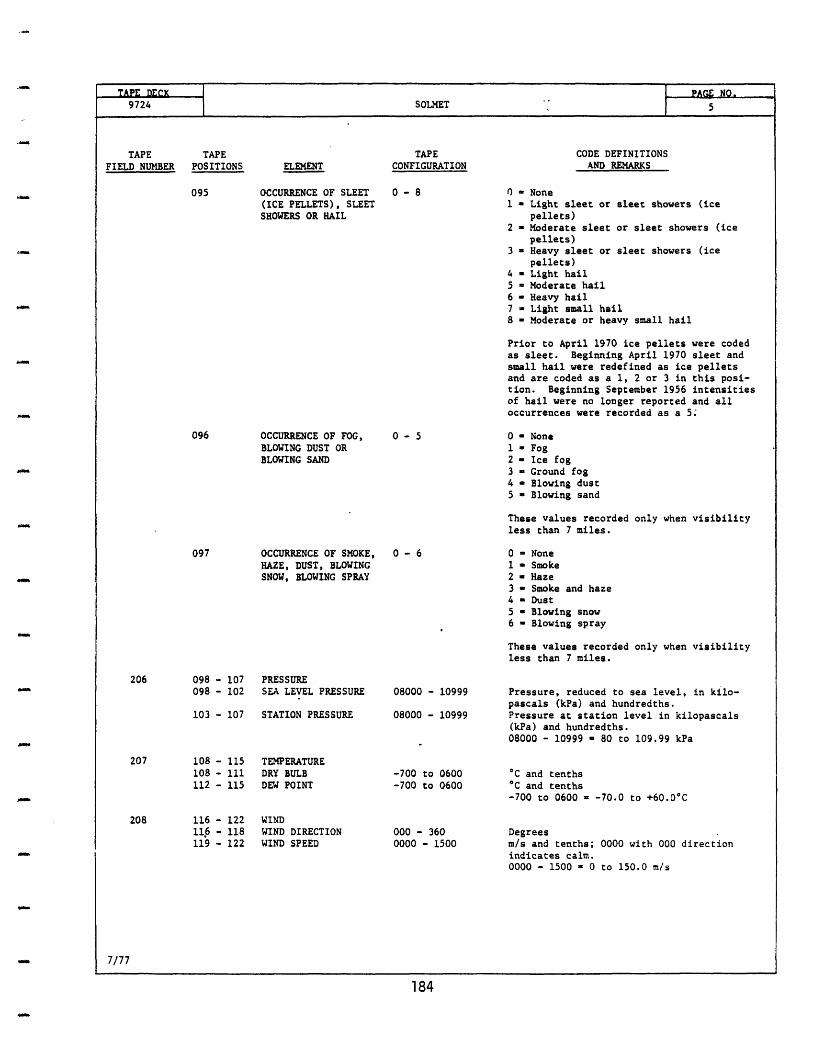
TAPE DCK PAGOL NOM9724 SOLMET 5
TAPECONFIGURATION
CODE DEFINITIONSAND REMARKS
OCCURRENCE OF SLEET(ICE PELLETS), SLEETSHOWERS OR HAIL
0-8 0 None1 - Light sleet or sleet showers (ice
pellets)2 - Moderate sleet or sleet showers (ice
pellets)3 - Heavy sleet or sleet showers (ice
pellets)4 - Light hail5 - Moderate hail6 - Heavy hail7 - Light small hail8 - Moderate or heavy small hail
Prior to April 1970 ice pellets were codedas sleet. Beginning April 1970 sleet andsmall hail were redefined as ice pelletsand are coded as a 1, 2 or 3 in this posi-tion. Beginning September 1956 intensitiesof hail were no longer reported and alloccurrences were recorded as a 5;
OCCURRENCE OF FOG,BLOWING DUST ORBLOWING SAND
OCCURRENCE OF SMOKE,HAZE, DUST, BLOWINGSNOW, BLOWING SPRAY
206 098 - 107 PRESSURE098 - 102 SEA LEVEL PRESSURE
103 - 107 STATION PRESSURE
0-5 0 - None1 - Fog2 - Ice fog3 - Ground fog4 - Blowing dust5 - Blowing sand
These values recordedless than 7 miles.
0-6 0 - None1 - Smoke2 - Haze3 - Smoke and haze4 - Dust5 - Blowing snow6 - Blowing spray
These values recordedless than 7 miles.
08000 - 10999
08000 - 10999
only when visibility
only when visibility
Pressure, reduced to sea level, in kilo-pascals (kPa) and hundredths.Pressure at station level in kilopascals(kPa) and hundredths.08000 - 10999 = 80 to 109.99 kPa
207 108 - 115 TEMPERATURE108 - 111 DRY BULB112 - 115 DEW POINT
208 116 - 122 WIND11 - 118 WIND DIRECTION119 - 122 WIND SPEED
-700 to 0600-700 to 0600
000 - 3600000 - 1500
°C and tenths°C and tenths-700 to 0600 =
Degreesm/s and tenths;indicates calm.0000 - 1500 - 0
-70.0 to +60.0°C
0000 with 000 direction
to 150.0 m/s
7/77
184
TAPEFIELD NUMBER
TAPEPOSITIONS ELEMENT
095
096
097
U
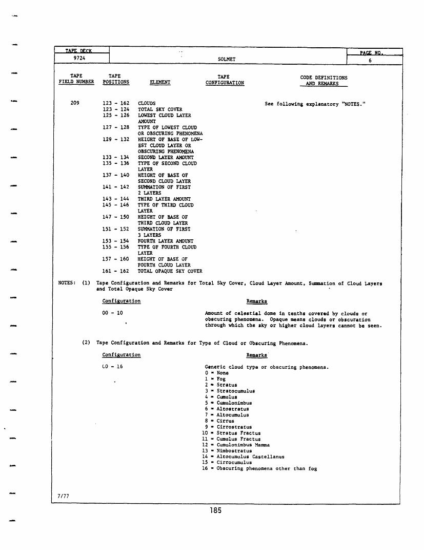
TAPECONFIGURATION
CODE DEFINITIONSAND REMARKS
209 123 - 162 CLOUDS123 - 124 TOTAL SKY COVER125 - 126 LOWEST CLOUD LAYER
AMOUNT127 - 128 TYPE OF LOWEST CLOUD
OR OBSCURING PHENOMENA129 - 132 HEIGHT OF BASE OF LOW-
EST CLOUD LAYER OROBSCURING PHENOMENA
133 - 134 SECOND LAYER AMOUNT135 - 136 TYPE OF SECOND CLOUD
LAYER137 - 140 HEIGHT OF BASE OF
SECOND CLOUD LAYER141 - 142 SUMMATION OF FIRST
2 LAYERS143 - 144 THIRD LAYER AMOUNT145 - 146 TYPE OF THIRD CLOUD
LAYER147 - 150 HEIGHT OF BASE OF
THIRD CLOUD LAYER151 - 152 SUMMATION OF FIRST
3 LAYERS153 - 154 FOURTH LAYER AMOUNT155 - 156 TYPE OF FOURTH CLOUD
LAYER157 - 160 HEIGHT OF BASE OF
FOURTH CLOUD LAYER161 - 162 TOTAL OPAQUE SKY COVER
NOTES: (1) Tape Configuration and Remarks for Tcand Total Opaque Sky Cover
Configuration
00 - 10
See following explanatory "NOTES."
)tal Sky Cover, Cloud Layer Amount, Summation of Cloud Layers
Remarks
Amount of celestial dome in tenths covered by clouds orobscuring phenomena. Opaque means clouds or obscurationthrough which the sky or higher cloud layers cannot be seen.
(2) Tape Configuration and Remarks for Type of Cloud or Obscuring Phenomena.
Configuration
CO - 16
Remarks
Generic cloud type or obscuring phenomena.0 - None1 = Fog2 - Stratus3 - Stratocumulus4 - Cumulus5 - Cumulonimbus6 - Altostratus7 - Altocumulus8 = Cirrus9 - Cirrostratus
10 = Stratus Fractus11 = Cumulus Fractus12 = Cumulonimbus Manmma13 - Nimbostratus14 - Altocumulus Castellanus15 - Cirrocumulus16 = Obscuring phenomena other than fog
7/77
185
TAPEFIELD NUMBER
TAPEPOSITIONS ELEMENT
I
9724 SOLMET 6
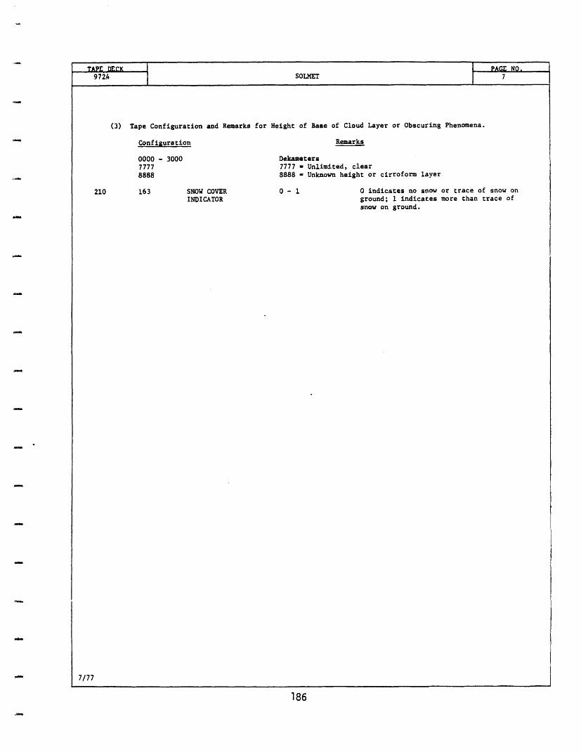
972.4 SOLMET 7
(3) Tape Configuration and Remarks for Height of Base of Cloud Layer or Obscuring Phenomena.
Configuration Remarks
0000 - 3000 Dekameters7777 7777 - Unlimited, clear8888 8888 - Unknown height or cirroform layer
210 163 SNOW COVER 0 - 1 0 indicates no snow or trace ofINDICATOR
snow on
ground; 1 indicates more than trace ofsnow on ground.
7/77
186
APPENDIX A5
W.M.O. CLOUD DEFINITION AND CLASSIFICATION
1. Cloud Classification
The W.M.O. classification [68] does not consider as a
classification criterion the forming process of the clouds; it
tries instead to consider their general appearance, their
obscuration characteristics, and their shape or particular
visible optical effects.* This is done to allow visual
recognition of the sky dome.
Principally, 10 genera of clouds are considered in
ascending order as follows:
1. Cumulonimbus
2. Cumulus
3. Stratus
4. Stratocumulus
5. Nimbostratus
6. Altostratus
*Reference [68] also reports photographs of the differenttypes of clouds.
187
7. Altocumulus
8. Cirrostratus
9. Cirrocumulus
10. Cirrus
Stratus and stratocumulus clouds are generally found in
the lower layer; altocumulus in the middle layer; and cirrus,
cirrocumulus and cirrostratus in the higher layer. Altostratus
clouds are generally located in the middle-higher layers.
Nimbostratus, cumulus, and cumulonimbus extend over more than
one layer, generally starting from the higher limit of the
lower layer.
The layer definition is aleatory, in the sense that it
varies, mainly with latitude. An approximate description of
the height of the layers, i.e., elevation of the inferior limit
of the layer, would be as follows (for temperate regions):
Low layer: surface to 2,000 m
Medium layer: from 2,000 to 8,000 m
High layer: from 5,000 to 14,000 m
In tropical regions, the highest layer maximum elevation
would be approximately 40 percent higher than in the
temperature regions, all the other layers being the same.
188
Every genus may be further divided into species and
varieties.
2. Cloud definition (from reference [68])
1 Cumulonimbus:
Heavy and dense cloud, with a considerable vertical
extent, in the form of a mountain or huge towers. At least
part of its upper portion is usually smooth, fibrous, or
striated, and nearly always flattened: this part often spreads
out in the shape of an anvil or vast plume. Under the base of
this cloud, which is often very dark, there are frequently low
ragged clouds either merged with it or not, and precipitation
sometimes in the form of virga.
Species or Varieties: Cumulonimbus mamma (among others)
2 Cumulus:
Detached clouds, generally dense and with sharp outlines,
developing vertically in the form of rising mounds, domes, or
towers, of which the bulging upper part often resembles a
cauliflower. The sunlit parts of these clouds are mostly
brilliant white. Their base is relatively dark and nearly
horizontal. Sometimes, cumulus is ragged.
Species or Varieties: Cumulus fractus (among others)
189
3 Stratus:
Generally gray cloud layer with a fairly uniform base . . .
When the Sun is visible through the cloud, its outline is
clearly discernible . . . Sometimes stratus appears in the form
of ragged patches.
Species or Varieties: Stratus fractus (among others)
4 Stratocumulus:
Gray or whitish, or both gray and whitish, patch, sheet or
layer of cloud which almost always has dark parts, composed of
tasselations, rounded masses, rolls, etc. which are nonfibrous
(except for virga) and which may or may not be merged; most of
the regularly arranged, small elements have an apparent width
of more than 5 degrees.
5 Nimbostratus:
Gray cloud layer, often dark, the appearance of which is
rendered diffuse by more or less continuously falling rain or
snow, which in most cases reaches the ground. It is thick
enough throughout to blot out the Sun. Low, ragged clouds
frequently occur below the layer, with which they may or may
not merge.
190
6 Altostratus:
Grayish or bluish cloud sheet or layer of striated,
fibrous, or uniform appearance, totally or partly covering the
sky, and having parts thin enough to reveal the Sun at least
vaguely as through ground glass . . .
7 Altocumulus:
White or gray, or both white and gray, patch, sheet or
layer of cloud, generally with shading, composed of laminae,
rounded masses, rolls, etc., which are sometimes partly fibrous
or diffuse and which may or may not be merged; most of the
regularly arranged small elements usually have an apparent
width of between one and five degrees.
Species or Varieties: Altocumulus castellanus (among
others)
8 Cirrostratus:
Transparent, whitish cloud veil of fibrous (hair-like) or
smooth appearance, totally or partly covering the sky .
9 Cirrocumulus:
Thin, white patch, sheet or layer of cloud without
shading, composed of very small elements in the form of grains,
ripples, etc., merged or separate and more or less regularly
arranged; most of the elements have an apparent width of less
than one degree.
191
10 Cirrus:
Detached clouds in the form of white, delicate filaments
or white or mostly white patches or narrow bands. These clouds
have a fibrous (hair-like) appearance.
192
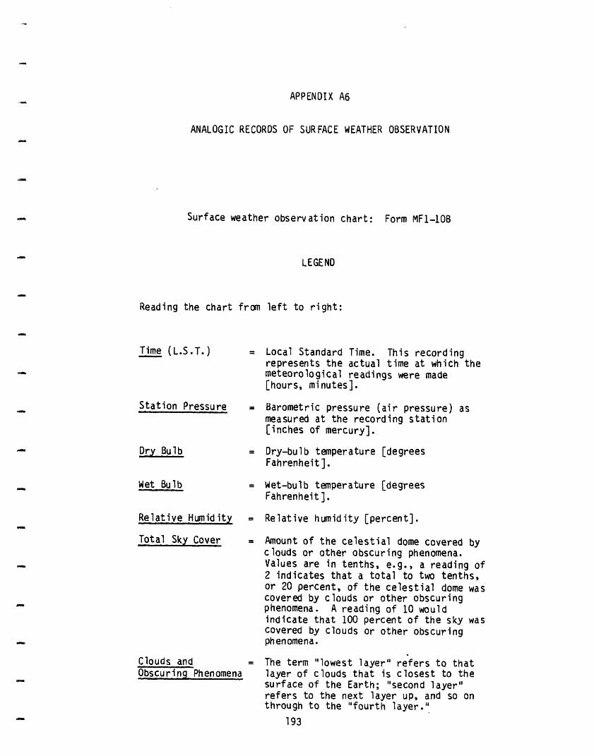
APPENDIX A6
ANALOGIC RECORDS OF SURFACE WEATHER OBSERVATION
Surface weather observation chart: Form MF1-1OB
LEGEND
Reading the chart from left to right:
Time (L.S.T.)
Station Pressure
Dry Bulb
Wet Bulb
Relative Humidity
Total Sky Cover
Clouds andObscuring Phenomena
= Local Standard Time. This recordingrepresents the actual time at which themeteorological readings were made[hours, minutes].
= Barometric pressure (air pressure) asmeasured at the recording station[inches of mercury].
= Dry-bulb temperature [degreesFahrenheit].
= Wet-bulb temperature [degreesFahrenheit].
= Relative humidity [percent].
- Amount of the celestial dome covered byclouds or other obscuring phenomena.Values are in tenths, e.g., a reading of2 indicates that a total to two tenths,or 20 percent, of the celestial dome wascovered by clouds or other obscuringphenomena. A reading of 10 wouldindicate that 100 percent of the sky wascovered by clouds or other obscuringphenomena.
The term "lowest layer" refers to thatlayer of clouds that is closest to thesurface of the Earth; "second layer"refers to the next layer up, and so onthrough to the "fourth layer."
193
-
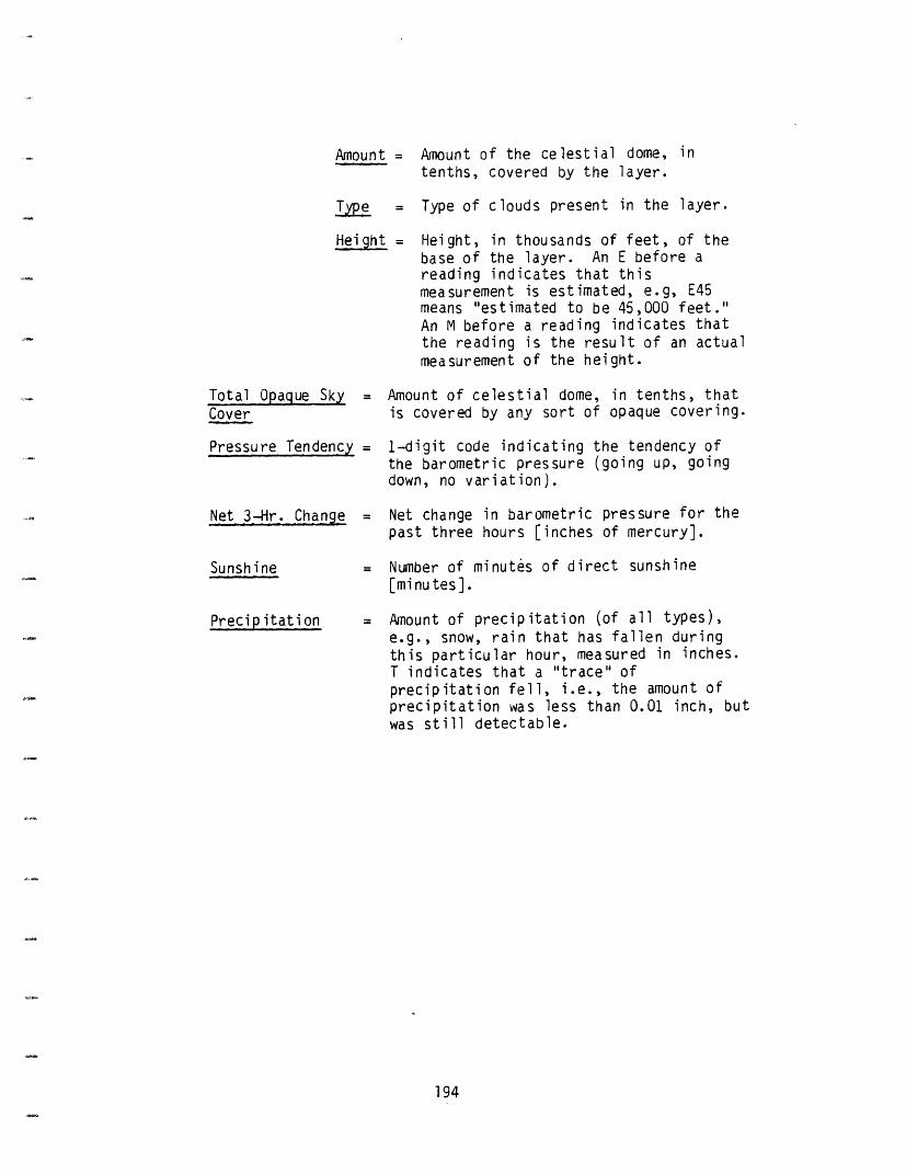
Amount = Amount of the celestial dome, intenths, covered by the layer.
Type = Type of clouds present in the layer.
Height = Height, in thousands of feet, of thebase of the layer. An E before areading indicates that thismeasurement is estimated, e.g, E45means "estimated to be 45,000 feet."An M before a reading indicates thatthe reading is the result of an actualmeasurement of the height.
Total Opaque SkyCover
Pressure Tendency
Net 3-Hr. Change
Sunshine
Precipitation
Amount of celestial dome, in tenths, thatis covered by any sort of opaque covering.
1-digit code indicating the tendency ofthe barometric pressure (going up, goingdown, no variation).
= Net change in barometric pressure for thepast three hours [inches of mercury].
= Number of minutes of direct sunshine[minutes].
= Amount of precipitation (of all types),e.g., snow, rain that has fallen duringthis particular hour, measured in inches.T indicates that a "trace" ofprecipitation fell, i.e., the amount ofprecipitation was less than 0.01 inch, butwas still detectable.
194
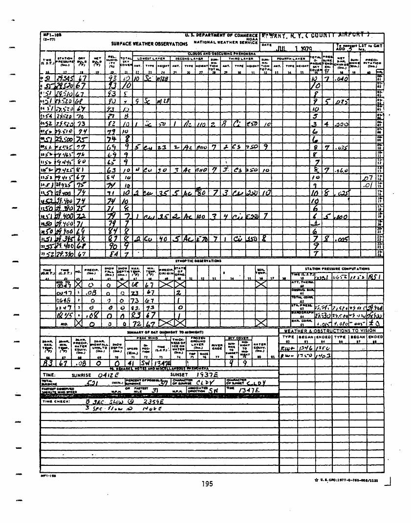
Ml.-O u...DEPATMiNT OFOMMERCE rIl l'~r. RT Y. ¢UeuI ulAInR FT )'(2.71 NOAASURFACE WEATHER OBSERVATIONS NATIONAL WEATHER SERVICE [T Te.. e LST L e G MT°'-JUL lq7q ADD. hr..
_g STATION DRY WET OTA LOWEST LAYER I CLOUDS 0 LAICSNAO OS ISCUU" C FRTN LAER lTOOTA. _ _=
19 II 2C 1 22 2 I IN 2I I l
A.-~~~~~~~~~~~~~tu~ ~~~~~~~~~~~A , ! IM 0i
.? ,. == .. == == =-:/' £. - ./ o- 4_ _ _-' I F0.',(4 Wi if.-.'zp
57/ j) r a 4 ̀ o 2 |1_= 8I~a_ ~l I d:~L~ " & L.~ 0709-
~-_,'~>~ ... ' ,. A = G . ' =o".
lsbS.' gi _~e wU~uD. b a _O _ 1_ __ _
.a 2 0 a a
71 1~J~.3b~?sS 1- 2y Yo 1v 7- i LQ. - s- -+ - --- - -=--£ -t- - -
,...,
4-e154!7 = X7 =_ _ ==
_ 7if 1 7 ~.~,,.c ~,j ~- /u 3 ,~ A 7 'es LAO /
_ a 1.~~ *, 4 ~q / t* I .... **7 *9 r 24SYNOPTIC OSSIEVATIONS
T im e TIoE NO i R . No S O X AtU.N M TA? Sol. STATION PREIWU1 COPUT&TOwSa FALL OF. TL.S.or) I... ) 0 - () ( 3 RI41 o 1? (L ..
___ 44 Al 47316 71 SO St 12 1S 1 1 '1 9MID .T/ m. O Imo. Q Q 73 i~I-7 ,- 61rv 1 67 1 1, ,6 , W I 7 1 .1 7 11
fl3 uz.1 6? 1'7 d O 0 1 1_1 _ 0 -____ I1A.eCa III
iM SURISE .V .I, , Z 1
I**_^s ~ ~ ~vumAR or DAY O4t"3 T ToMDNIT) WEI i L6QSTRCTIONS TO VISION'^'°. ° mum. PRECIP. 3p51*3* *35Q3 30 ^^^ @IINO EATEN i34JL.o .L -_ -L 11 asTEml I CC. EOW U L) E 23 1iE GAGE TO
- . .. ) . m I .T awa.) _ ,. I , I . . I4, 41 S 1d'4 9 - -
TIME: SUNRISE o4 Z E SUNSET I37 - -
'110TAL 001,00,Powot" c L Y, I CN Y A' -CTIAts.. or o o '*~Kgl O&, r a TO Ori ~14l(TMT)co
i "No iet a i .P.P. "Lit NP 9 I I /347£
TIMaSCHlECKp: 5, JAC -i 2--3 ·- Iru r63 4 .- el ,
* U. PO:l1977-76-0o/lS J195Ikfr-IO
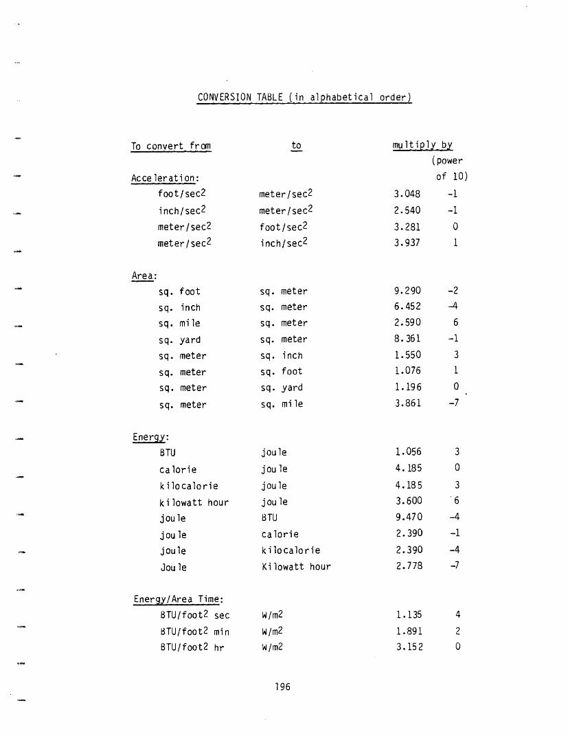
CONVERSION TABLE (in alphabetical order)
To convert from
Acceleration:
foot/sec2
inch/sec 2
meter/sec 2
meter/sec2
Area:
sq.
sq.
sq.
sq.
sq.
sq.
sq.
sq.
foot
inch
mile
yard
meter
meter
meter
meter
to
meter/sec 2
meter/sec 2
foot/sec 2
inch/sec 2
sq.
sq.
sq.
sq.
sq.
sq.
sq.
sq.
meter
meter
meter
meter
inch
foot
yard
mile
multiply by
(power
of 10)
3.048 -1
2.540 -1
3.281 0
3.937 1
9.290
6. 452
2.590
8. 361
1.550
1.076
1.196
3.861
-2
-4
6
-1
3
1
0
-7
Energy:
BTU
calorie
kilocalorie
kilowatt hour
joule
joule
joule
Joule
Energy/Area Time:
BTU/foot2 sec
BTU/foot2 min
BTU/foot2 hr
joule
jou le
joule
jou le
BTU
calorie
kilocalorie
Kilowatt hour
w/m2
Wlm2
w/m2
196
1.056
4. 185
4.185
3.600
9.470
2.390
2.390
2.778
3
0
3
6
-4
-1
-4
-7
4
2
0
1.135
1.891
3.152
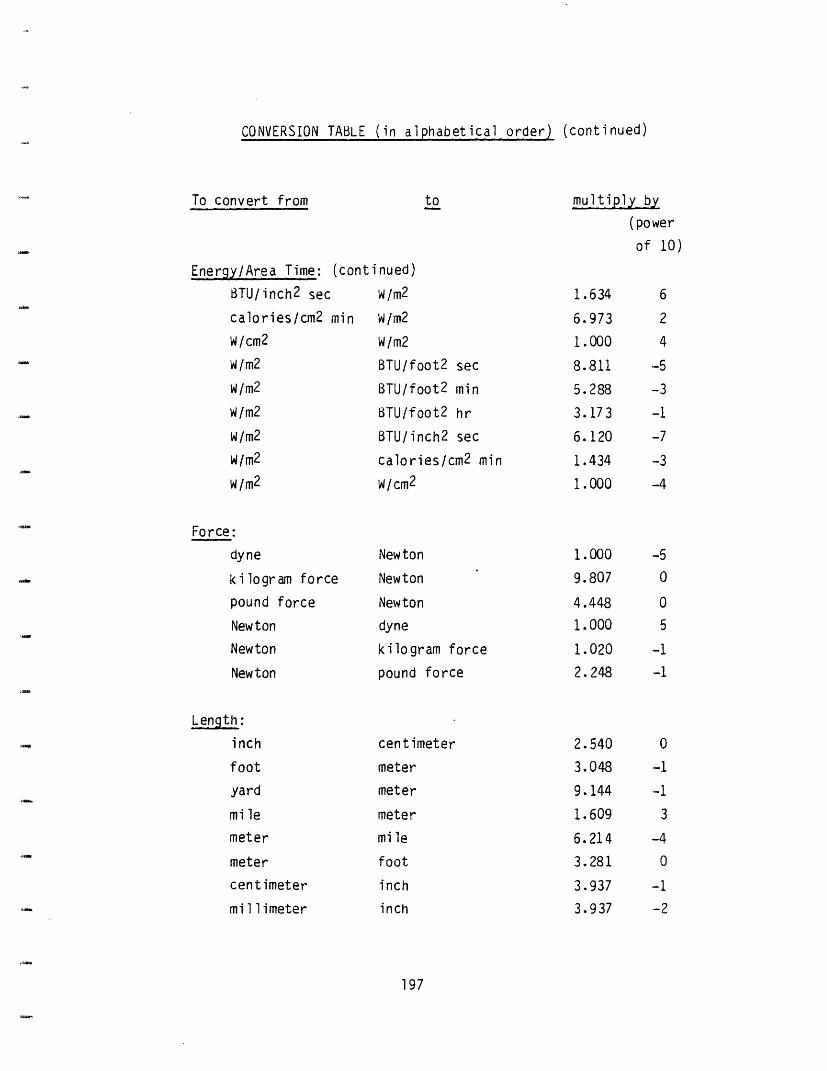
CONVERSION TABLE (in alphabetical order) (continued)
To convert from to multiply by
(power
of 10)
Energy/Area Time: (continued)
BTU/inch2 sec W/m2
calories/cm2 min W/m2
W/cm 2 W/m2
w/m2 BTU/foot2 sec
W/m2 BTU/foot2 min
W/m2 tTU/foot2 hr
W/m2 BTU/inch2 sec
W/m2 calories/cm2 min
w/m2 W/cm 2
Force:
dyne
kilogram force
pound force
Newton
Newton
Newton
Length:
inch
foot
yard
mile
meter
meter
centimeter
millimeter
Newton
Newton
Newton
dyne
kilogram force
pound force
centimeter
meter
meter
meter
mile
foot
inch
inch
197
1.634
6.973
1.000
8.811
5.288
3.173
6.120
1.434
1.000
6
2
4
-5
-3
-I
-7
-3
-4
1.000
9.807
4.448
1.000
1.020
2.248
2.540
3.048
9.144
1.609
6.214
3.281
3.937
3.937
-5
0
0
5
-1
-1
0
-1
-1
3
-4
0
-1
-2
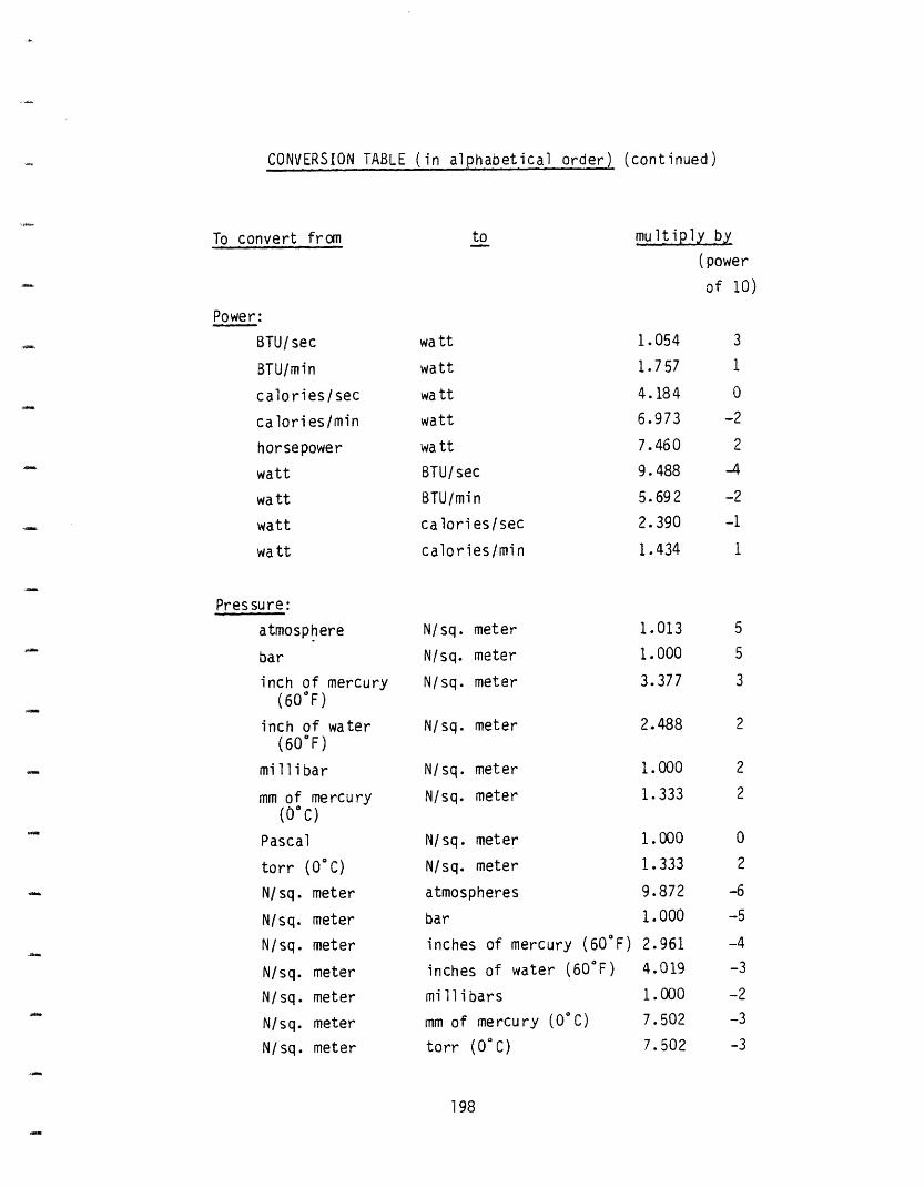
CONVERSION TABLE (in alphabetical order) (continued)
To convert from
Power:
BTU/sec
BTU/min
calories/sec
calories/min
horsepower
watt
watt
watt
watt
to
watt
watt
watt
watt
watt
BTU/sec
BTU/min
calories/sec
calories/min
multiply by
(power
of 10)
1.054
1.757
4. 184
6.973
7.460
9.488
5.692
2.390
1.434
3
1
0
-2
2-4
-2
-1
1
Pressure:
atmosphere
bar
inch of mercury(60 F)
inch of water(60°F)
millibar
mm of mercury(O C)
Pascal
torr (O0C)
N/sq. meter
N/sq. meter
N/sq. meter
N/sq. meter
N/sq. meter
N/sq. meter
N/sq. meter
N/sq.
N/sq.
N/sq.
meter
meter
meter
N/sq. meter
N/sq.
N/sq.
meter
meter
N/sq. meter
N/sq. meter
atmospheres
bar
inches of mercury (600F)
inches of water (60°F)
millibars
mm of mercury (O0C)
torr (O°C)
198
1.013
1.000
3.377
5
5
3
2.488 2
2
2
1.000
1.333
1.000
1.333
9.872
1.000
2.961
4.019
1.000
7.502
7.502
0
2
-6
-5
-4-3
-2
-3
-3
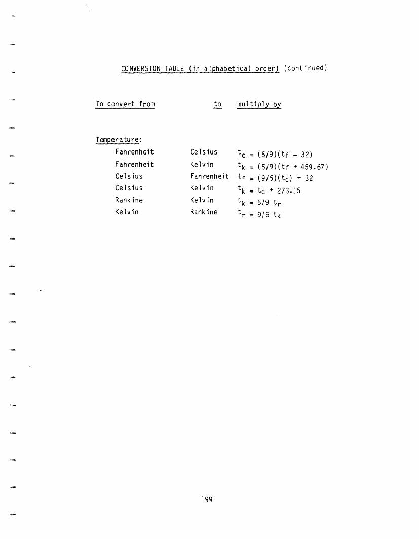
CONVERSION TABLE (in alphabetical order) (continued)
To convert from to multiply by
Temperature:
Fahrenheit
Fahrenheit
Celsius
Celsius
Rank ine
Kelvin
Celsius
Kelvin
Fahrenheit
Kelvin
Kelvin
Rank ine
tc =
tk =
tf =
tk =
tk =
tr =
(5/9)(tf - 32)
(5/9)(tf + 459.67)
(9/5)(tc) + 32
tc + 273.15
5/9 tr
9/5 tk
199
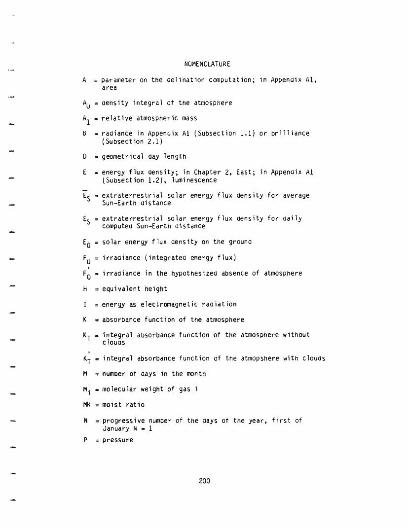
NOMENCLATURE
A = parameter on the delination computation; in Appendix Al,area
A0 = density integral of the atmosphere
A1 = relative atmospheric mass
b = radiance in Appendix Al (Subsection 1.1) or brilliance(Subsection 2.1)
D = geometrical day length
E = energy flux density; in Chapter 2, East; in Appendix Al(Subsection 1.2), luminescence
ES = extraterrestrial solar energy flux density for averageSun-Earth distance
ES = extraterrestrial solar energy flux density for dailycomputed Sun-Earth distance
E0 = solar energy flux density on the ground
F0 = irradiance (integrated energy flux)
FO = irradiance in the hypothesized absence of atmosphere
H = equivalent height
I = energy as electromagnetic radiation
K = absorbance function of the atmosphere
KT = integral absorbance function of the atmosphere withoutclouds
KT = integral absorbance function of the atmopshere with clouds
M = number of days in the month
M i = molecular weight of gas i
MR = moist ratio
N = progressive number of the days of the year, first ofJanuary N = 1
P = pressure
200
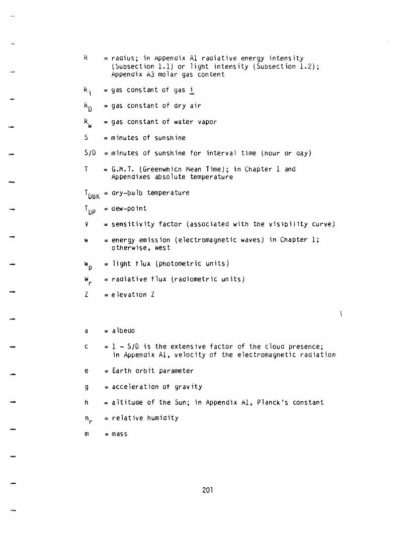
R = radius; in Appendix Al radiative energy intensity(Subsection 1.1) or light intensity (Subsection 1.2);Appendix A3 molar gas content
ki = gas constant of gas i
kD = gas constant of dry air
RW = gas constant of water vapor
S = minutes of sunshine
S/D = minutes of sunshine for interval time (hour or day)
T = G.M.T. (Greenwhich Mean Time); in Chapter 1 andAppendixes absolute temperature
TDbK = ary-bulb temperature
TDp : dew-point
V = sensitivity factor (associated with the visibility curve)
h = energy emission (electromagnetic waves) in Chapter 1;otherwise, west
p = light tlux (photometric units)
Wr = radiative flux (radiometric units)r
Z = elevation Z
a = albedo
c = 1 - S/D is the extensive factor of the cloua presence;in Appendix Al, velocity of the electromagnetic radiation
e = Earth orbit parameter
g = acceleration ot gravity
h = altituoe of the Sun; in Appendix Al, Planck's constant
hr = relative humidity
m = mass
201
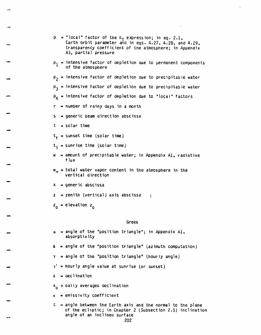
p = "local" factor of the KT expression; in eq. 2.1,Earth orbit parameter ana in eqs. 4.27, 4.28, and 4.29,transparency coefficient of the atmosphere; in AppendixA3, partial pressure
pi = intensive factor of epletion aue to permanent componentsof the atmosphere
P2 = intensive factor of depletion aue to precipitable water
P3 = intensive tactor of depletion due to precipitable water
P4 = intensive factor of depletion due to "local" factors
r = number of rainy days in a month
s = generic beam direction abscissa
t = solar time
tf =sunset time (solar time)
ti = sunrise time (solar time)
w = amount of precipitable water; in Appendix Al, radiativetflux
w. = total water vapor content in the atmosphere in thevertical direction
x = generic abscissa
z = zenith (vertical) axis abscissa
zo = elevation zo
Greek
a = angle of the "position triangle"; in Appendix Al,absorptivity
=B angle of the "position triangle" (azimuth computation)
Y = angle of the "position triangle" (hourly angle)
y' = hourly angle value at sunrise (or sunset)
6 = declination
6o = daily averagea eclination
c = emissivity coefficient
c = angle between the Earth axis and the normal to the planeof the ecliptic; in Chapter 2 (Subsection 2.5) inclinationangle of an inclined surface
202
A_
A_
I*
= total cloua cover
n -total opaque cloud cover
e = zenith angle
A = wavelength; in astronomical computations, longitude
= anomaly of the Earth in its orbit
= 3.1415927
p = density; in Chapters 1 and 2, aaily average value of theSun-Earth distance; in Appendix Al, retlectivitycoefficient
p = average between aphelion ana perihelion of Sun-Earthdistance
a = Stetan-boltzmann's constant
T = transmission coefficient
= latituae
+ = function symbol
= azimuth
=' = orientation angle of an inclined surface ("azimuth" of thenormal)
w = solia ang e
Superscripts
= degrees
= minutes
Subscripts
D = dry air
E = Earth
i = incident; in Appendixes, i-th gas
203
1 = local
m = meridian
M1 = moist air
max = maximum
S = Sun
W = water vapor
Z = elevation Z
0 = zero
204
REFERENCES
1. G. Russo, "Analytical Models and Numerical SimulationCodes for Solar Energy Systems' Engineers (I),"Fourth Course on Solar Energy Conversion,International Center for Theoretical Physics, Italy,1977.
2. G. Russo, "Passive and Active Systems Radiation Dynamics,"Act of the Congress SAIE 77, Italy, 1977.
3. A. Russo and G. Russo, "Analytical Models and NumericalSimulation Codes for Solar Energy Systems Engineering(II)," Fourth Course on Solar Energy Conversion,International Center for Theoretical Physics, Italy,1977.
4. G. Russo, "Design of Solar Energy Conditioning Systems,"Technical Report, Polytechnic of Torino, School ofEngineering, Torino, Italy, 1975.
5. G. Russo, "Solar Collectors: Testing Loop Design," FIATC.R.F. Technical Report No. 528/75/lmr, 1975.
6. G. Russo and F. Demichelis, "Transmission Solar FocusingCollectors," Lettere al Nuovo Cimento, 19 5, 1977,pp. 145-51.
7. G. Russo and L. Matteoli, "Energy Programming for theEnergy Independence of the Island of Pantelleria,"Pantelleria Administration, Trapani, Italy, 1978.
8. G. Russo, "Analytical Model and Simulation Codes for theSolar Input Determination: Irradiation Maps,"Journal of Solar Energy 21, 1978, pp. 201-210.
9. K.Y. Kondratyev, "The Radiant Energy of the Sun,"Gidrometeoizdat, Leningrad, 1954.
10. R.M. Goody, Atmospheric Radiation: Theoretical Basis,London: Oxford University Press, 1964.
11. M.I. Budyko, et al., "The Heat Balance of the Earth'sSurface," Zvest Akademie, URSS Geographical Series 3,1954.
12. G.A.W. Rutgers, Temperature Radiation of Solyds,Handbuch der Physic 26.
205
13. S. Chandrasekhar, Radiative Transfer, London: OxfordUniversity Press, 1950.
14. S.L. Valley, Handbook of Geophysics and SpaceEnvironments, Bedford, Massachusetts: Air ForceCambridge Research Laboratories, 1965.
15. U.S. Hydrographic Office, "Tables of Computed Altitude andAzimuth," Publication No. 214, 1940.
16. NASA, "Solar Electromagnetic Radiation," SP-8005, 1971.
17. M.P. Thekaekara and A.J. Drummond, "Standard Values forthe Solar Constant and its Spectral Components," Nat.Phys. Sci. 229 6, 1971.
18. R.M. Goody, "A Statistical Model for Water VaporAbsorption," Quart. J. Roy. Meteorol. Soc. 78 336,1954.
19. G.N. Plass, "The Influence of Numerous Low-IntensitySpectral Lines on Band Absorptance," Appl. Opt. 3 7,1964.
20. L.D. Kaplan, "A Quasi-Statistical Approach to theCalculation of Atmospheric Transmission," Proc.Toronto Meteorol. Conf., Toronto, 1953.
21. G.N. Plass, "Models of Spectral Band Absorption," J. Am.Opt. Soc. 58 10, 1958.
22. G.N. Plass, "Useful Representation for Measurements ofSpectral Band Absorption," J. Am. Opt. Soc., 50 9,1960.
23. K.Y. Kondratyev, et al., "A New Radiation Chart," Geofis.Para. Appl. 49, 1961.
24. K.Y. Kondratyev, Radiant Solar Energy, Leningrad, 1954.
25. E. Glueckauf, "The Composition of Atmospheric Air,"Compendium of Meteorology, 1951, pp. 1-11.
26. R.M. Goody, The Physics of the Stratosphere, OxfordUniversity Press, 1954.
27. F. Moller, et al., "On the Heat Balance of theTroposphere," Final Report Contract AF 61-052-18,Mainz.
206
28. A. Angstrom, "Absorption of Solar Radiation by AtmosphericWater Vapor," Arkiv Geophysik 3, 23, 1961.
29. E. Vigroux, et al., "Resultats d'Observations de l'OzoneAtmospherique par le Methode Infra-rouge," Ann.Geophys. 19 31, 1963.
30. D.E. Burch, et al., "Infrared Absorption by Carbon DioxideWater Vapor and Minor Atmospheric Constituents,"Contract AF 19-604-2633, Ohio State University, 1962.
31. H.C. Van de Hulst, Light Scattering by Small Particles,New York: J. Wiley, 1964.
32. K. Bullrich, "Scattered Radiation in the Atmosphere andthe Natural Aerosol," Adv. Geophys. 10, 1964.
33. Proceedings of the International InterdisciplinaryConference on Electromagnetic Scattering, Oxford,England: Pergamon Press, 1963.
34. A. Angstrom, "The Parameters of Atmospheric Turbidity,"Tellus 16 1, 1963.
35. E.M. Fuegelson, "Radiative Process in the Stratus Clouds,"Nauke, Moscow, 1964.
36. H. Korb and F. Moller, "Theoretical Investigation ofEnergy Gain by Absorption of Solar Radiation inClouds," Tech. Dep. DA-91-591-EVC-1612, Munchen, 1962.
37. L.M. Romanova, "Radiation Field in the Plane Layers of aTurbid Medium with a Strong Unisotropic Scattering,"Opt. Spectr. (English Translation), 13 3 and 6,USSR, 1963.
38. .J. Norris, "Correlation of Solar Radiation with Clouds,"Solar Energy 12 107, 1968.
39. G.T. Trewartha, An Introduction to Climate, New York:McGraw Hill, 1954.
40. S.J. Reddy, "An Empirical Method for Estimating Sunshinefrom Total Cloud Amount," Solar Energy 15, 1974.
41. S.J. Reddy, "An Empirical Method of Estimation of TotalSolar Radiation," Solar Energy 13 289, 1971.
42. S.J. Reddy, "An Empirical Method of Estimation of NetRadiation Intensity," Solar Energy 13 291, 1971.
207
43. A. Angstrom, "On the Computation of Global Radiation fromRecords of Sunshine," Arkiv for Geophysik, 1957.
44. J.N. Black, et al., "Solar Radiation and the Duration ofSunshine," Royal Meteorological Society, 1954.
45. Acta of the Congress, The Sun in the Service of Mankind,Paris, 1973.
46. F.E. Lumb, "The Influence of Clouds on Hourly Amounts ofTotal Solar Radiation," Royal Meteorological Society,1964.
47. Data of the "Aeronautica Militare Italiana, IspettoratoTelecomunicazioni ed Assistenza al Volo," ServizioMeteorologico, Rome.
48. Data of the Meteorological Observatory of Pino Torinese,Torino, Italy.
49. G. Bozza, "Tabelle di Solarita," La Termotecnica Ricerche7, 1958.
50. K.H. Pogosyan, The Air Envelope of the Earth, Gimitz,Leningrad (English Translation: Israel Program forScientific Translation, Jerusalem, 1965), 1962.
51. V.G. Kastrov, "To the Problem of Solar RadiationAttenuation in an Ideal Atmosphere," Meteorol. 47 4,1930.
52. V.G. Kastrov, Solar Radiation in the Troposphere in theCase of Absolutely Clean and Dry Air," Trans. Centr.Aerol. Obs. 16, 1956.
53. S.I. Sivkov, "Attenuation of Solar Radiation in an IdealAtmosphere," Trans. Main Geophysics Obs. 169, 1965.
54. Peter H. Stone, Massachusetts Institute of Technology,private communication, 1979.
55. T. Sesamori, et al., "Radiation Budget of the SouthernHemisphere," Meteor. Mous. 13, 9-23.
56. T.H. Vander Hear and V.E. Susni, "Measurements of theEarth's Radiation Budget from Satellites duringFive-Year Period," J. Atmos. Sci. 28, pp. 305-315.
57. R.C.J. Sommerville, et al., "The GISS Model of the GlobalAtmosphere, J. Atmos. Sci. 31, pp. 84-117.
208
58. N.E. Ter-Markariantz, "Mean Daily Albedo Values," Trans.Main Geophys. Obs. 100, 1960.
59. A.P. Koptev, "Albedo of Clouds, Water, Snow, and Ice,"Trans. Arct. Antarct. Inst. 229, 1961.
60. A.A. Lacis and J.E. Hansen, "A Parametrization for theAbsorption of Solar Radiation in the Atmosphere," J.Atmos. Sci. 31, 1974, pp. 118-133.
61. SOLMET, Vol. I: User's Manual, U.S. Department ofCommerce, National Oceanic and AtmosphericAdministration, Environmental Data and InformationService, National Climatic Center, Asheville, NorthCarolina, 1978. T-9724.
62. SOLMET, Vol. II: Final Report, U.S. Department ofCommerce, National Oceanic and AtmosphericAdministration, Environmental Data and InformationService, National Climatic Center, Asheville, NorthCarolina, 1978. TD-9724.
63. National Weather Service Observing Handbook No. 3: SolarRadiation Observations, 1977.
64. W.R. Seguin, "Documentation for the 1977 Global andDiffuse Solar Radiation Data," National ClimaticCenter, Asheville, North Carolina.
65. C.M. Randall and M.E. Whitson, Jr., "Final Report HourlyInsolation and Meteorological Data Bases includingImproved Direct Insolation Estimates," The AerospaceCorporation, Report No. ATR-78(7592)-1.
66. M.P. Thekerara and A. J. Drummond, "Standard Values forthe zlar Constant and its Spectral Components,"Nature Physical Science 229, 1971.
67. C. Frohlich, et al., "The Third International Comparisonsof Phyroheliometers and a Comparison of RadiometricScales," Solar Energy 14, 1973.
68. World Meteorological Organization Cloud Atlas, 1957.
209