Embed Size (px)
Citation preview
Software Reliability:Runtime Verification
Martin Leucker– and the whole ISP team –
Institute for Software EngineeringUniversitat zu Lubeck
Riga, 21.07. – 04.08.14
Martin Leucker Basoti, 2014 1/117
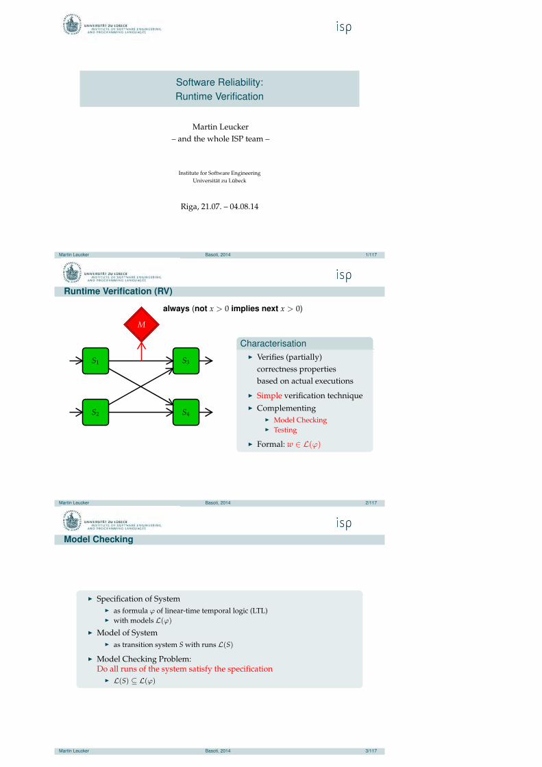
Runtime Verification (RV)
S1
S2
S3
S4
M
always (not x > 0 implies next x > 0)
Characterisation◮ Verifies (partially)
correctness propertiesbased on actual executions
◮ Simple verification technique◮ Complementing
◮ Model Checking◮ Testing
◮ Formal: w ∈ L(ϕ)
Martin Leucker Basoti, 2014 2/117
Model Checking
◮ Specification of System◮ as formula ϕ of linear-time temporal logic (LTL)◮ with models L(ϕ)
◮ Model of System◮ as transition system S with runs L(S)
◮ Model Checking Problem:Do all runs of the system satisfy the specification
◮ L(S) ⊆ L(ϕ)
Martin Leucker Basoti, 2014 3/117
Model Checking versus RV
◮ Model Checking: infinite words◮ Runtime Verification: finite words
◮ yet continuously expanding words
◮ In RV: Complexity of monitor generation is of less importance thancomplexity of the monitor
◮ Model Checking: White-Box-Systems
◮ Runtime Verification: also Black-Box-Systems
Martin Leucker Basoti, 2014 4/117
Testing
Testing: Input/Output Sequence◮ incomplete verification technique
◮ test case: finite sequence of input/output actions
◮ test suite: finite set of test cases
◮ test execution: send inputs to the system and check whether the actualoutput is as expected
Testing: with Oracle◮ test case: finite sequence of input actions
◮ test oracle: monitor
◮ test execution: send test cases, let oracle report violations
◮ similar to runtime verification
Martin Leucker Basoti, 2014 5/117
Testing versus RV
◮ Test oracle manual
◮ RV monitor from high-level specification (LTL)
◮ Testing:
How to find good test suites?
◮ Runtime Verification:How to generate good monitors?
Martin Leucker Basoti, 2014 6/117

OutlineRuntime VerificationRuntime Verification for LTL
LTL over Finite, Completed WordsLTL over Finite, Non-Completed Words: ImpartialityLTL over Non-Completed Words: AnticipationLTL over Infinite Words: With AnticipationGeneralisations: LTL with modulo ConstraintsMonitorable PropertiesLTL with a Predictive SemanticsLTL wrap-up
ExtensionsTesting Temporal Properties with RV: jUnitRVMonitoring Systems/LoggingSteeringDiagnosis
IdeasRV and Diagnosis
ConclusionMartin Leucker Basoti, 2014 7/117
Presentation outlineRuntime VerificationRuntime Verification for LTL
LTL over Finite, Completed WordsLTL over Finite, Non-Completed Words: ImpartialityLTL over Non-Completed Words: AnticipationLTL over Infinite Words: With AnticipationGeneralisations: LTL with modulo ConstraintsMonitorable PropertiesLTL with a Predictive SemanticsLTL wrap-up
ExtensionsTesting Temporal Properties with RV: jUnitRVMonitoring Systems/LoggingSteeringDiagnosis
IdeasRV and Diagnosis
ConclusionMartin Leucker Basoti, 2014 8/117
Runtime Verification
Definition (Runtime Verification)Runtime verification is the discipline of computer science that deals with thestudy, development, and application of those verification techniques thatallow checking whether a run of a system under scrutiny (SUS) satisfies orviolates a given correctness property.
Its distinguishing research effort lies in synthesizing monitors from high levelspecifications.
Definition (Monitor)A monitor is a device that reads a finite trace and yields a certain verdict.
A verdict is typically a truth value from some truth domain.
Martin Leucker Basoti, 2014 9/117
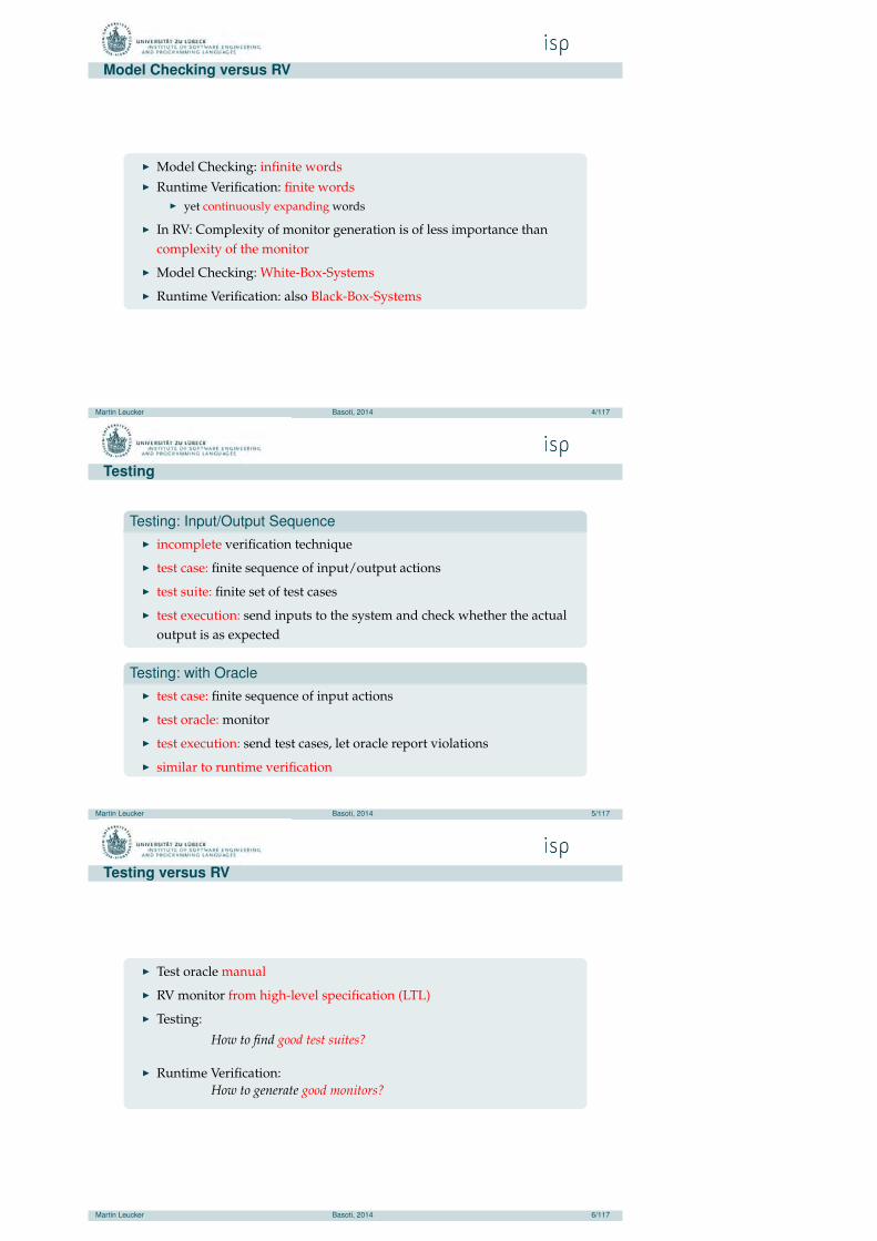
Taxonomy
runtimeverification
trace
finite
finite non-completed
infinite
integration
inline
outline
stage
online
offline
interference
invasive
non-invasive
steering
activepassive
monitoring
input/output
behavior
state se-quence
eventsequence
applicationarea
safetychecking
security
informationcollection
performanceevaluation
Martin Leucker Basoti, 2014 10/117
Presentation outlineRuntime VerificationRuntime Verification for LTL
LTL over Finite, Completed WordsLTL over Finite, Non-Completed Words: ImpartialityLTL over Non-Completed Words: AnticipationLTL over Infinite Words: With AnticipationGeneralisations: LTL with modulo ConstraintsMonitorable PropertiesLTL with a Predictive SemanticsLTL wrap-up
ExtensionsTesting Temporal Properties with RV: jUnitRVMonitoring Systems/LoggingSteeringDiagnosis
IdeasRV and Diagnosis
ConclusionMartin Leucker Basoti, 2014 11/117
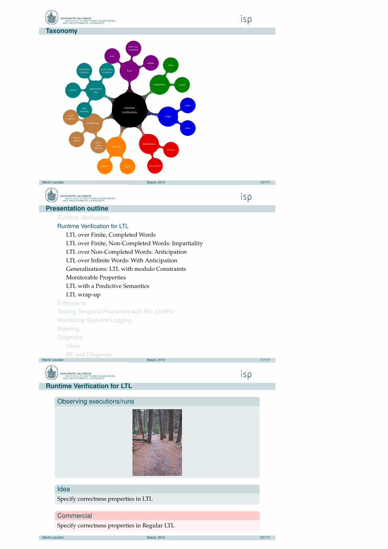
Runtime Verification for LTL
Observing executions/runs
IdeaSpecify correctness properties in LTL
CommercialSpecify correctness properties in Regular LTL
Martin Leucker Basoti, 2014 12/117
Runtime Verification for LTL
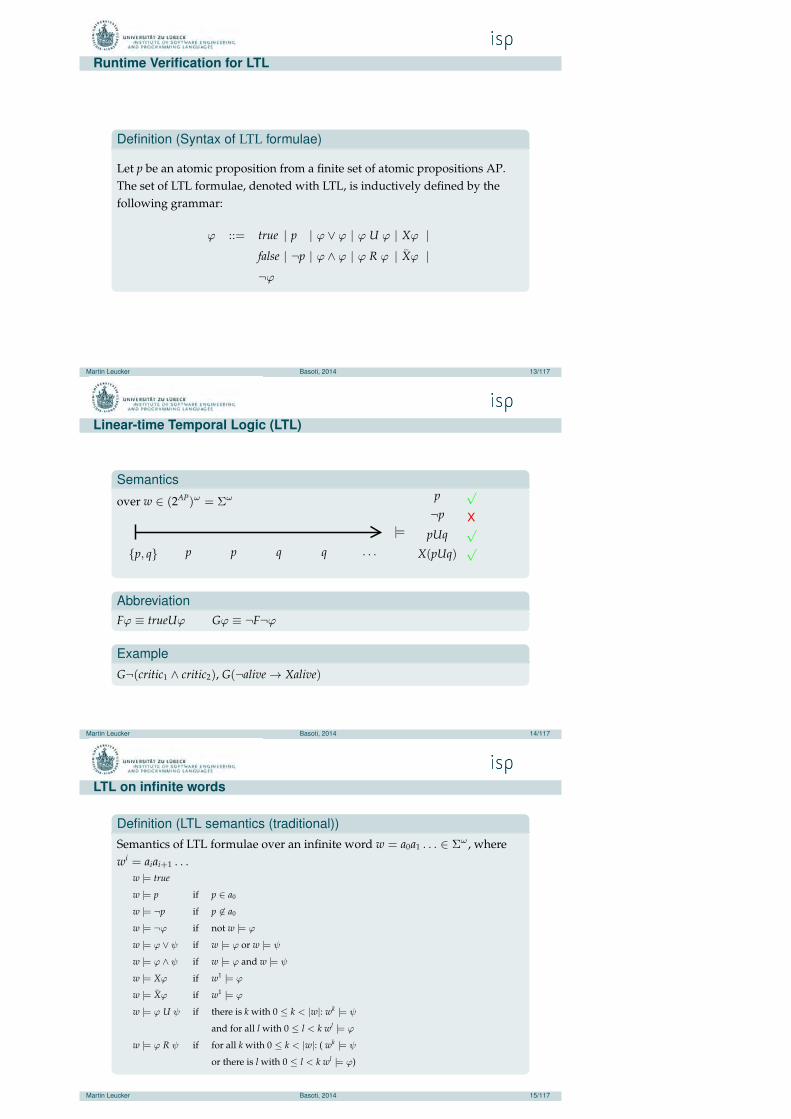
Definition (Syntax of LTL formulae)
Let p be an atomic proposition from a finite set of atomic propositions AP.The set of LTL formulae, denoted with LTL, is inductively defined by thefollowing grammar:
ϕ ::= true | p | ϕ ∨ ϕ | ϕ U ϕ | Xϕ |false | ¬p | ϕ ∧ ϕ | ϕ R ϕ | Xϕ |¬ϕ
Martin Leucker Basoti, 2014 13/117
Linear-time Temporal Logic (LTL)
Semantics
over w ∈ (2AP)ω = Σω
{p, q} p p q q . . .
|=
p
¬p
pUq
X(pUq)
√
X√√
AbbreviationFϕ ≡ trueUϕ Gϕ ≡ ¬F¬ϕ
ExampleG¬(critic1 ∧ critic2), G(¬alive → Xalive)
Martin Leucker Basoti, 2014 14/117
LTL on infinite words
Definition (LTL semantics (traditional))Semantics of LTL formulae over an infinite word w = a0a1 . . . ∈ Σω , wherewi = aiai+1 . . .
w |= true
w |= p if p ∈ a0
w |= ¬p if p 6∈ a0
w |= ¬ϕ if not w |= ϕ
w |= ϕ ∨ ψ if w |= ϕ or w |= ψ
w |= ϕ ∧ ψ if w |= ϕ and w |= ψ
w |= Xϕ if w1 |= ϕ
w |= Xϕ if w1 |= ϕ
w |= ϕ U ψ if there is k with 0 ≤ k < |w|: wk |= ψ
and for all l with 0 ≤ l < k wl |= ϕ
w |= ϕ R ψ if for all k with 0 ≤ k < |w|: ( wk |= ψ
or there is l with 0 ≤ l < k wl |= ϕ)
Martin Leucker Basoti, 2014 15/117

LTL for the working engineer??
Simple??“LTL is for theoreticians—but for practitioners?”
SALTStructured Assertion Language for Temporal Logic“Syntactic Sugar for LTL” [Bauer, L., Streit@ICFEM’06]
Martin Leucker Basoti, 2014 16/117
SALT – http://www.isp.uni-luebeck.de/salt
Martin Leucker Basoti, 2014 17/117
Runtime Verification for LTL
IdeaSpecify correctness properties in LTL
Definition (Syntax of LTL formulae)
Let p be an atomic proposition from a finite set of atomic propositions AP.The set of LTL formulae, denoted with LTL, is inductively defined by thefollowing grammar:
ϕ ::= true | p | ϕ ∨ ϕ | ϕ U ϕ | Xϕ |false | ¬p | ϕ ∧ ϕ | ϕ R ϕ | Xϕ |¬ϕ
Martin Leucker Basoti, 2014 18/117
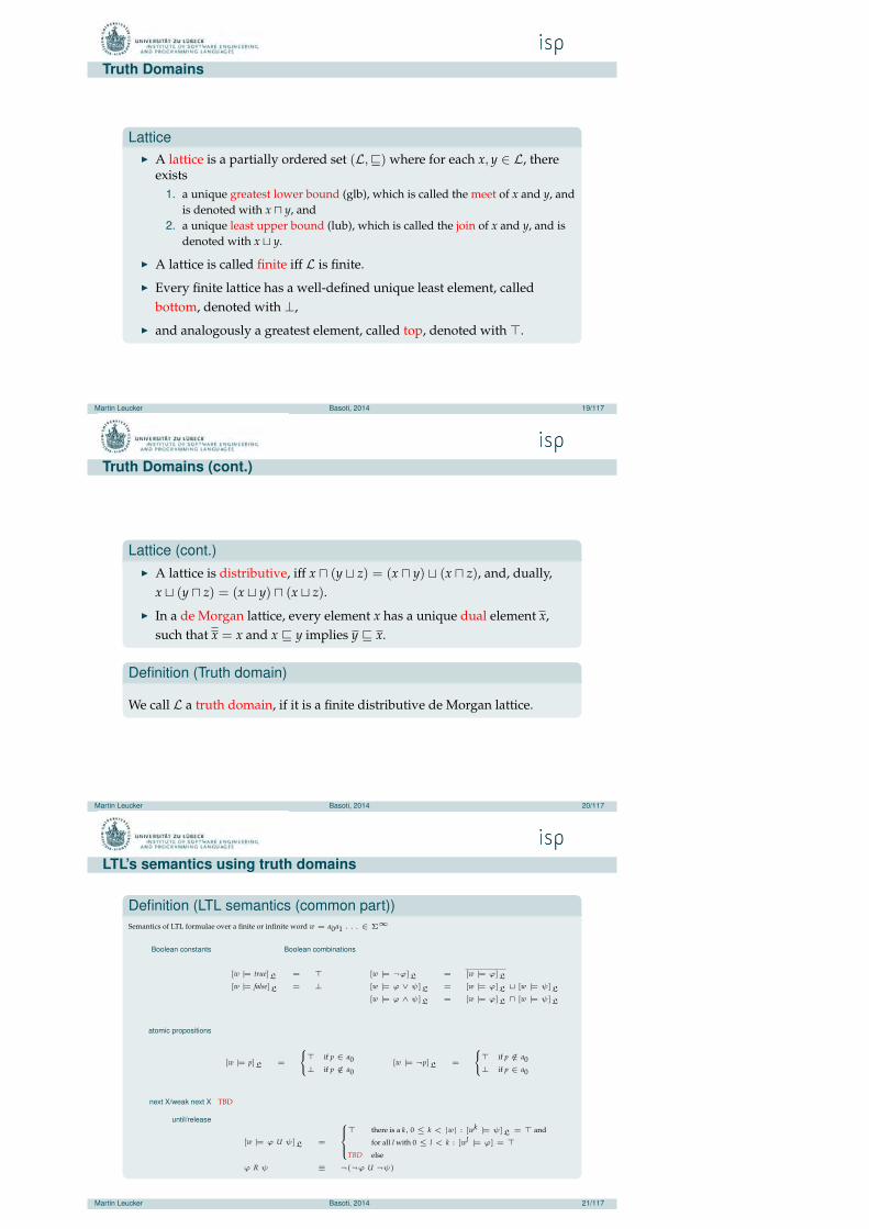
Truth Domains
Lattice◮ A lattice is a partially ordered set (L,⊑) where for each x, y ∈ L, there
exists1. a unique greatest lower bound (glb), which is called the meet of x and y, and
is denoted with x ⊓ y, and2. a unique least upper bound (lub), which is called the join of x and y, and is
denoted with x ⊔ y.
◮ A lattice is called finite iff L is finite.
◮ Every finite lattice has a well-defined unique least element, calledbottom, denoted with ⊥,
◮ and analogously a greatest element, called top, denoted with ⊤.
Martin Leucker Basoti, 2014 19/117
Truth Domains (cont.)
Lattice (cont.)◮ A lattice is distributive, iff x ⊓ (y ⊔ z) = (x ⊓ y) ⊔ (x ⊓ z), and, dually,
x ⊔ (y ⊓ z) = (x ⊔ y) ⊓ (x ⊔ z).
◮ In a de Morgan lattice, every element x has a unique dual element x,such that x = x and x ⊑ y implies y ⊑ x.
Definition (Truth domain)
We call L a truth domain, if it is a finite distributive de Morgan lattice.
Martin Leucker Basoti, 2014 20/117
LTL’s semantics using truth domains
Definition (LTL semantics (common part))Semantics of LTL formulae over a finite or infinite word w = a0a1 . . . ∈ Σ∞
Boolean constants
[w |= true]L = ⊤[w |= false]L = ⊥
Boolean combinations
[w |= ¬ϕ]L = [w |= ϕ]L
[w |= ϕ ∨ ψ]L = [w |= ϕ]L ⊔ [w |= ψ]L
[w |= ϕ ∧ ψ]L = [w |= ϕ]L ⊓ [w |= ψ]L
atomic propositions
[w |= p]L =
⊤ if p ∈ a0⊥ if p /∈ a0
[w |= ¬p]L =
⊤ if p /∈ a0⊥ if p ∈ a0
next X/weak next X TBD
until/release
[w |= ϕ U ψ]L =
⊤ there is a k, 0 ≤ k < |w| : [wk |= ψ]L = ⊤ and
for all l with 0 ≤ l < k : [wl |= ϕ] = ⊤TBD else
ϕ R ψ ≡ ¬(¬ϕ U ¬ψ)
Martin Leucker Basoti, 2014 21/117

LTL on finite words
Application area: Specify properties of finite word
Martin Leucker Basoti, 2014 23/117
LTL on finite words
Definition (FLTL)Semantics of FLTL formulae over a word u = a0 . . . an−1 ∈ Σ∗
next
[u |= Xϕ]F =
[u1 |= ϕ]F if u1 6= ǫ
⊥ otherwise
weak next
[u |= Xϕ]F =
[u1 |= ϕ]F if u1 6= ǫ
⊤ otherwise
Martin Leucker Basoti, 2014 24/117
Monitoring LTL on finite words
(Bad) Ideajust compute semantics. . .
Martin Leucker Basoti, 2014 25/117
LTL on finite, but not completed words
Application area: Specify properties of finite but expanding word
Martin Leucker Basoti, 2014 27/117
LTL on finite, but not completed words
Be Impartial!◮ go for a final verdict (⊤ or ⊥) only if you really know
◮ be a man: stick to your word
Martin Leucker Basoti, 2014 28/117
LTL on finite, but not complete words
Impartiality implies multiple valuesEvery two-valued logic is not impartial.
Definition (FLTL)Semantics of FLTL formulae over a word u = a0 . . . an−1 ∈ Σ∗
next
[u |= Xϕ]F =
[u1 |= ϕ]F if u1 6= ǫ
⊥p otherwise
weak next
[u |= Xϕ]F =
[u1 |= ϕ]F if u1 6= ǫ
⊤p otherwise
Martin Leucker Basoti, 2014 29/117
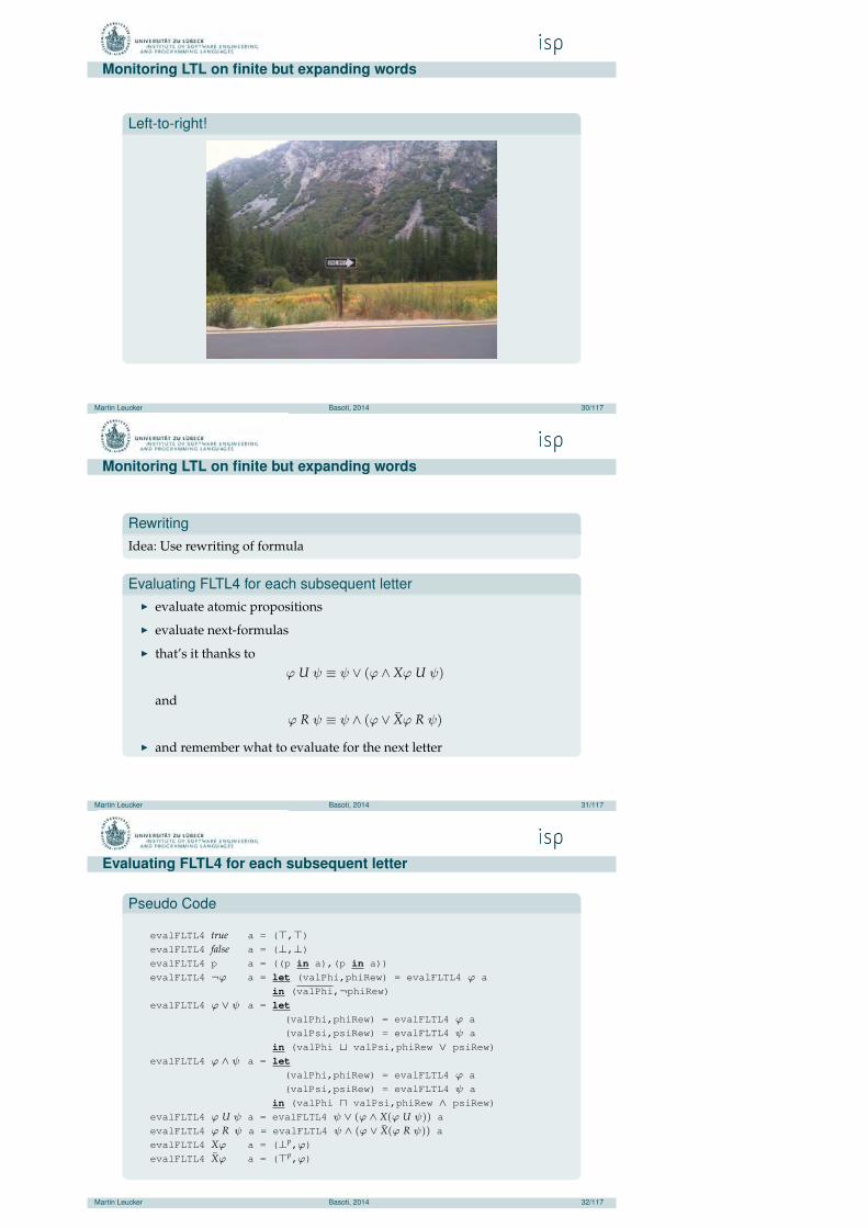
Monitoring LTL on finite but expanding words
Left-to-right!
Martin Leucker Basoti, 2014 30/117
Monitoring LTL on finite but expanding words
RewritingIdea: Use rewriting of formula
Evaluating FLTL4 for each subsequent letter◮ evaluate atomic propositions
◮ evaluate next-formulas
◮ that’s it thanks toϕ U ψ ≡ ψ ∨ (ϕ ∧ Xϕ U ψ)
andϕ R ψ ≡ ψ ∧ (ϕ ∨ Xϕ R ψ)
◮ and remember what to evaluate for the next letter
Martin Leucker Basoti, 2014 31/117
Evaluating FLTL4 for each subsequent letter
Pseudo Code
evalFLTL4 true a = (⊤,⊤)
evalFLTL4 false a = (⊥,⊥)
evalFLTL4 p a = ((p in a),(p in a))
evalFLTL4 ¬ϕ a = let (valPhi,phiRew) = evalFLTL4 ϕ a
in (valPhi,¬phiRew)evalFLTL4 ϕ ∨ ψ a = let
(valPhi,phiRew) = evalFLTL4 ϕ a
(valPsi,psiRew) = evalFLTL4 ψ a
in (valPhi ⊔ valPsi,phiRew ∨ psiRew)
evalFLTL4 ϕ ∧ ψ a = let(valPhi,phiRew) = evalFLTL4 ϕ a
(valPsi,psiRew) = evalFLTL4 ψ a
in (valPhi ⊓ valPsi,phiRew ∧ psiRew)
evalFLTL4 ϕ U ψ a = evalFLTL4 ψ ∨ (ϕ ∧ X(ϕ U ψ)) a
evalFLTL4 ϕ R ψ a = evalFLTL4 ψ ∧ (ϕ ∨ X(ϕ R ψ)) a
evalFLTL4 Xϕ a = (⊥p,ϕ)
evalFLTL4 Xϕ a = (⊤p,ϕ)
Martin Leucker Basoti, 2014 32/117
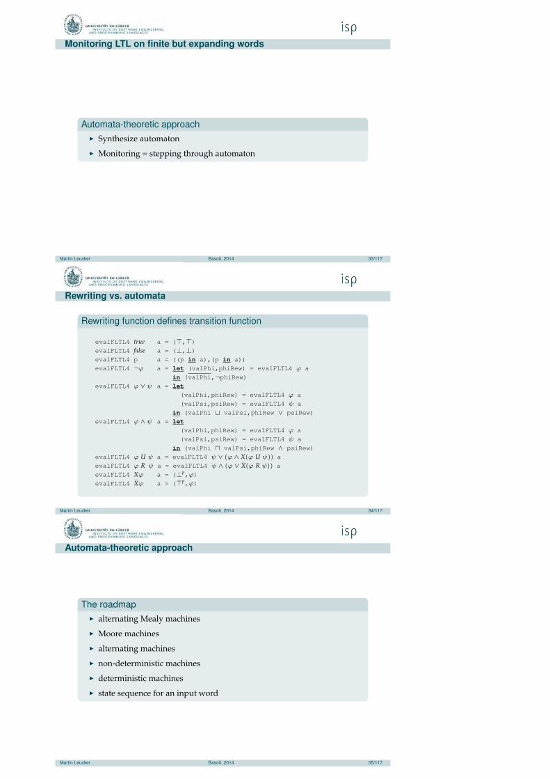
Monitoring LTL on finite but expanding words
Automata-theoretic approach◮ Synthesize automaton
◮ Monitoring = stepping through automaton
Martin Leucker Basoti, 2014 33/117
Rewriting vs. automata
Rewriting function defines transition function
evalFLTL4 true a = (⊤,⊤)
evalFLTL4 false a = (⊥,⊥)
evalFLTL4 p a = ((p in a),(p in a))
evalFLTL4 ¬ϕ a = let (valPhi,phiRew) = evalFLTL4 ϕ a
in (valPhi,¬phiRew)evalFLTL4 ϕ ∨ ψ a = let
(valPhi,phiRew) = evalFLTL4 ϕ a
(valPsi,psiRew) = evalFLTL4 ψ a
in (valPhi ⊔ valPsi,phiRew ∨ psiRew)
evalFLTL4 ϕ ∧ ψ a = let(valPhi,phiRew) = evalFLTL4 ϕ a
(valPsi,psiRew) = evalFLTL4 ψ a
in (valPhi ⊓ valPsi,phiRew ∧ psiRew)
evalFLTL4 ϕ U ψ a = evalFLTL4 ψ ∨ (ϕ ∧ X(ϕ U ψ)) a
evalFLTL4 ϕ R ψ a = evalFLTL4 ψ ∧ (ϕ ∨ X(ϕ R ψ)) a
evalFLTL4 Xϕ a = (⊥p,ϕ)
evalFLTL4 Xϕ a = (⊤p,ϕ)
Martin Leucker Basoti, 2014 34/117
Automata-theoretic approach
The roadmap◮ alternating Mealy machines
◮ Moore machines
◮ alternating machines
◮ non-deterministic machines
◮ deterministic machines
◮ state sequence for an input word
Martin Leucker Basoti, 2014 35/117
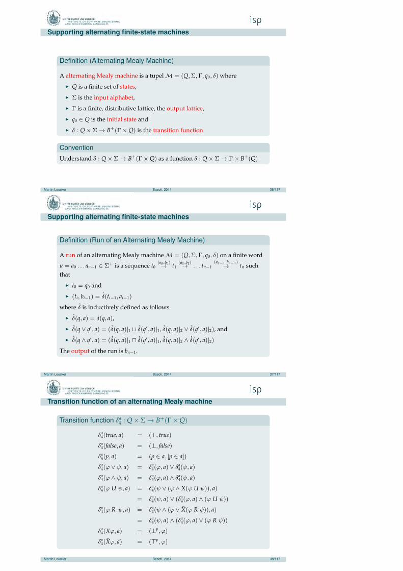
Supporting alternating finite-state machines
Definition (Alternating Mealy Machine)
A alternating Mealy machine is a tupel M = (Q,Σ,Γ, q0, δ) where
◮ Q is a finite set of states,
◮ Σ is the input alphabet,
◮ Γ is a finite, distributive lattice, the output lattice,
◮ q0 ∈ Q is the initial state and
◮ δ : Q × Σ → B+(Γ× Q) is the transition function
Convention
Understand δ : Q × Σ → B+(Γ× Q) as a function δ : Q × Σ → Γ× B+(Q)
Martin Leucker Basoti, 2014 36/117
Supporting alternating finite-state machines
Definition (Run of an Alternating Mealy Machine)
A run of an alternating Mealy machine M = (Q,Σ,Γ, q0, δ) on a finite word
u = a0 . . . an−1 ∈ Σ+ is a sequence t0(a0,b0)→ t1
(a1,b1)→ . . . tn−1(an−1,bn−1)→ tn such
that
◮ t0 = q0 and
◮ (ti, bi−1) = δ(ti−1, ai−1)
where δ is inductively defined as follows
◮ δ(q, a) = δ(q, a),
◮ δ(q ∨ q′, a) = (δ(q, a)|1 ⊔ δ(q′, a)|1, δ(q, a)|2 ∨ δ(q′, a)|2), and
◮ δ(q ∧ q′, a) = (δ(q, a)|1 ⊓ δ(q′, a)|1, δ(q, a)|2 ∧ δ(q′, a)|2)The output of the run is bn−1.
Martin Leucker Basoti, 2014 37/117
Transition function of an alternating Mealy machine
Transition function δa4 : Q × Σ → B+(Γ× Q)
δa4(true, a) = (⊤, true)
δa4(false, a) = (⊥, false)
δa4(p, a) = (p ∈ a, [p ∈ a])
δa4(ϕ ∨ ψ, a) = δa
4(ϕ, a) ∨ δa4(ψ, a)
δa4(ϕ ∧ ψ, a) = δa
4(ϕ, a) ∧ δa4(ψ, a)
δa4(ϕ U ψ, a) = δa
4(ψ ∨ (ϕ ∧ X(ϕ U ψ)), a)
= δa4(ψ, a) ∨ (δa
4(ϕ, a) ∧ (ϕ U ψ))
δa4(ϕ R ψ, a) = δa
4(ψ ∧ (ϕ ∨ X(ϕ R ψ)), a)
= δa4(ψ, a) ∧ (δa
4(ϕ, a) ∨ (ϕ R ψ))
δa4(Xϕ, a) = (⊥p, ϕ)
δa4(Xϕ, a) = (⊤p, ϕ)
Martin Leucker Basoti, 2014 38/117

Anticipatory Semantics
Consider possible extensions of the non-completed word
Martin Leucker Basoti, 2014 40/117
LTL for RV [BLS@FSTTCS’06]
Basic idea◮ LTL over infinite words is commonly used for specifying correctness
properties
◮ finite words in RV:prefixes of infinite, so-far unknown words
◮ re-use existing semantics
3-valued semantics for LTL over finite words
[u |= ϕ] =
⊤ if ∀σ ∈ Σω : uσ |= ϕ
⊥ if ∀σ ∈ Σω : uσ 6|= ϕ
? else
Martin Leucker Basoti, 2014 42/117
Impartial Anticipation
Impartial◮ Stay with ⊤ and ⊥
Anticipatory◮ Go for ⊤ or ⊥◮ Consider XXXfalse
ǫ |= XXXfalse
a |= XXfalse
aa |= Xfalse
aaa |= false
[ǫ |= XXXfalse] =
⊤ if ∀σ ∈ Σω : ǫσ |= XXXfalse
⊥ if ∀σ ∈ Σω : ǫσ 6|= XXXfalse
? elseMartin Leucker Basoti, 2014 43/117
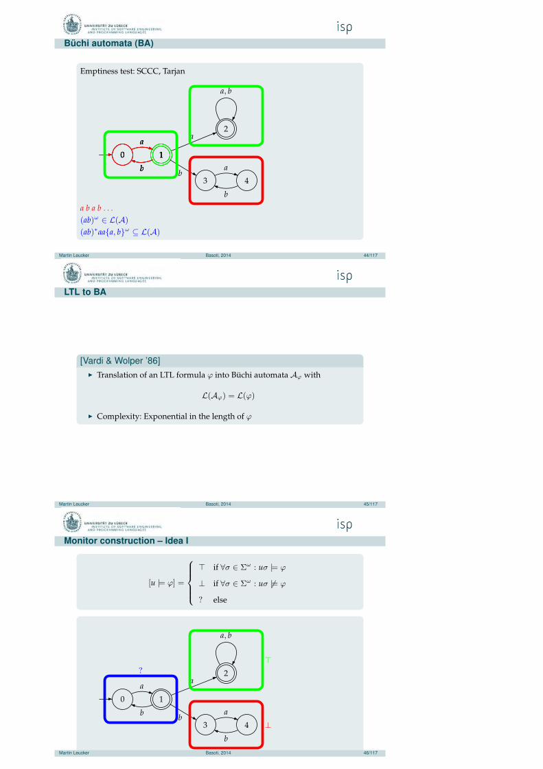
Buchi automata (BA)
Emptiness test: SCCC, Tarjan
000 111
2
3 4
aaa
bbb
a
a, b
ba
b
a b a b . . .(ab)ω ∈ L(A)
(ab)∗aa{a, b}ω ⊆ L(A)
Martin Leucker Basoti, 2014 44/117
LTL to BA
[Vardi & Wolper ’86]◮ Translation of an LTL formula ϕ into Buchi automata Aϕ with
L(Aϕ) = L(ϕ)
◮ Complexity: Exponential in the length of ϕ
Martin Leucker Basoti, 2014 45/117
Monitor construction – Idea I
[u |= ϕ] =
⊤ if ∀σ ∈ Σω : uσ |= ϕ
⊥ if ∀σ ∈ Σω : uσ 6|= ϕ
? else
0 1
2
3 4
a
b
a
a, b
ba
b
⊥
⊤?
Martin Leucker Basoti, 2014 46/117
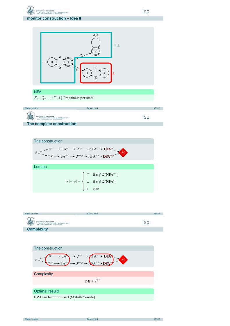
monitor construction – Idea II
0 1
2
3 4
a
b
a
a, b
ba
b
⊥
6= ⊥
NFAFϕ : Qϕ → {⊤,⊥} Emptiness per state
Martin Leucker Basoti, 2014 47/117
The complete construction
The construction
ϕ BAϕ Fϕ NFAϕ
¬ϕ BA¬ϕ F¬ϕ NFA¬ϕ
ϕDFAϕ
DFA¬ϕ
DFAϕ
DFA¬ϕM
Lemma
[u |= ϕ] =
⊤ if u /∈ L(NFA¬ϕ)
⊥ if u /∈ L(NFAϕ)
? else
Martin Leucker Basoti, 2014 48/117
Complexity
The construction
ϕ BAϕ Fϕ NFAϕ
¬ϕ BA¬ϕ F¬ϕ NFA¬ϕ
ϕDFAϕ
DFA¬ϕ
DFAϕ
DFA¬ϕM
Complexity
|M| ≤ 22|ϕ|
Optimal result!FSM can be minimised (Myhill-Nerode)
Martin Leucker Basoti, 2014 49/117
On-the-fly Construction
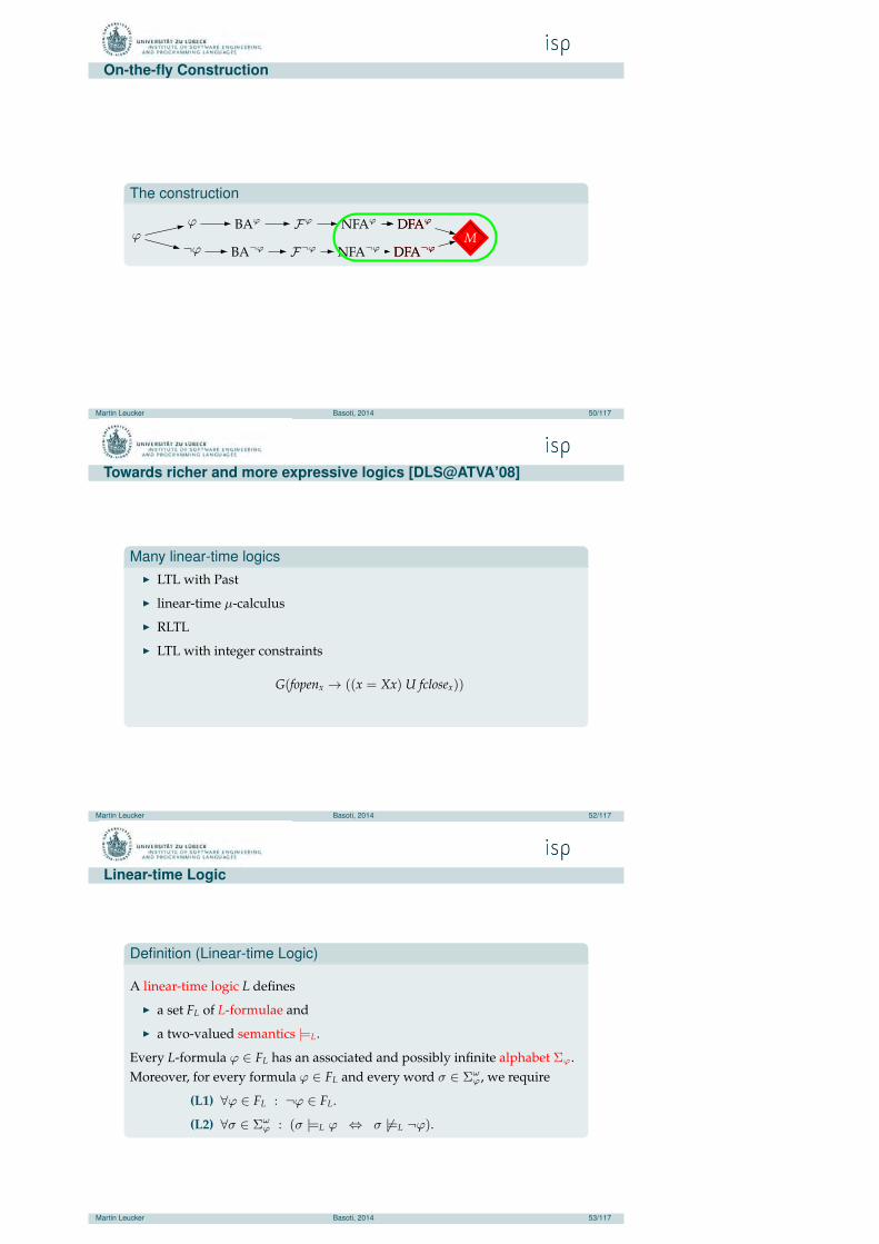
The construction
ϕ BAϕ Fϕ NFAϕ
¬ϕ BA¬ϕ F¬ϕ NFA¬ϕ
ϕDFAϕ
DFA¬ϕ
DFAϕ
DFA¬ϕM
Martin Leucker Basoti, 2014 50/117
Towards richer and more expressive logics [DLS@ATVA’08]
Many linear-time logics◮ LTL with Past
◮ linear-time µ-calculus
◮ RLTL
◮ LTL with integer constraints
G(fopenx → ((x = Xx) U fclosex))
Martin Leucker Basoti, 2014 52/117
Linear-time Logic
Definition (Linear-time Logic)
A linear-time logic L defines
◮ a set FL of L-formulae and
◮ a two-valued semantics |=L.
Every L-formula ϕ ∈ FL has an associated and possibly infinite alphabet Σϕ.Moreover, for every formula ϕ ∈ FL and every word σ ∈ Σω
ϕ, we require
(L1) ∀ϕ ∈ FL : ¬ϕ ∈ FL.
(L2) ∀σ ∈ Σωϕ : (σ |=L ϕ ⇔ σ 6|=L ¬ϕ).
Martin Leucker Basoti, 2014 53/117
Anticipation Semantics
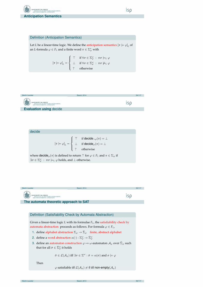
Definition (Anticipation Semantics)
Let L be a linear-time logic. We define the anticipation semantics [π |= ϕ]L ofan L-formula ϕ ∈ FL and a finite word π ∈ Σ∗
ϕ with
[π |= ϕ]L =
⊤ if ∀σ ∈ Σωϕ : πσ |=L ϕ
⊥ if ∀σ ∈ Σωϕ : πσ 6|=L ϕ
? otherwise
Martin Leucker Basoti, 2014 54/117
Evaluation using decide
decide
[π |= ϕ]L =
⊤ if decide¬ϕ(π) = ⊥⊥ if decideϕ(π) = ⊥? otherwise
where decideϕ(π) is defined to return ⊤ for ϕ ∈ FL and π ∈ Σϕ if∃σ ∈ Σω
ϕ : πσ |=L ϕ holds, and ⊥ otherwise.
Martin Leucker Basoti, 2014 55/117
The automata theoretic approach to SAT
Definition (Satisfiability Check by Automata Abstraction)
Given a linear-time logic L with its formulae FL, the satisfiability check byautomata abstraction proceeds as follows. For formula ϕ ∈ FL,
1. define alphabet abstraction Σϕ → Σϕ finite, abstract alphabet
2. define a word abstraction α(·) : Σωϕ → Σω
ϕ
3. define an automaton construction ϕ 7→ ω-automaton Aϕ over Σϕ suchthat for all σ ∈ Σω
ϕ it holds
σ ∈ L(Aϕ) iff ∃σ ∈ Σω : σ = α(σ) and σ |= ϕ
Thenϕ satisfiable iff L(Aϕ) 6= ∅ iff non-empty(Aϕ)
Martin Leucker Basoti, 2014 56/117
From finite to infinite
Definition (extrapolate)
extrapolate(π) ={α(πσ)0...i | i + 1 = |π|, σ ∈ Σω
}
Definition (Accuracy of Abstract Automata)
accuracy of abstract automata property holds, if, for all π ∈ Σ∗,
◮ (∃σ : πσ |=L ϕ) ⇒ (∃π∃σ : πσ ∈ L(Aϕ)) with π ∈ extrapolate(π),
◮ (∃σ : πσ ∈ L(Aϕ)) ⇒ (∃π∃σ : πσ |=L ϕ) with π ∈ extrapolate(π).
Martin Leucker Basoti, 2014 57/117
Non-incremental version
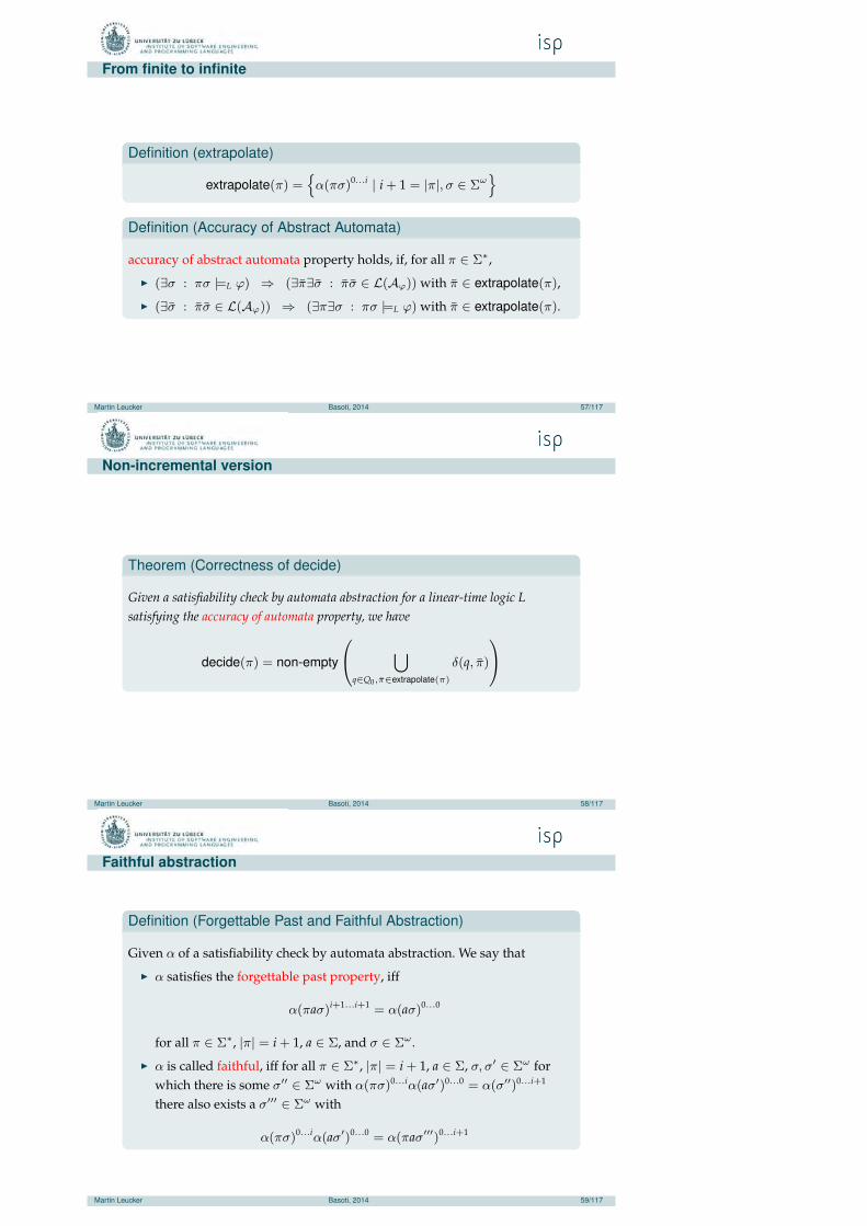
Theorem (Correctness of decide)
Given a satisfiability check by automata abstraction for a linear-time logic Lsatisfying the accuracy of automata property, we have
decide(π) = non-empty
⋃
q∈Q0,π∈extrapolate(π)
δ(q, π)
Martin Leucker Basoti, 2014 58/117
Faithful abstraction
Definition (Forgettable Past and Faithful Abstraction)
Given α of a satisfiability check by automata abstraction. We say that
◮ α satisfies the forgettable past property, iff
α(πaσ)i+1...i+1 = α(aσ)0...0
for all π ∈ Σ∗, |π| = i + 1, a ∈ Σ, and σ ∈ Σω .
◮ α is called faithful, iff for all π ∈ Σ∗, |π| = i + 1, a ∈ Σ, σ, σ′ ∈ Σω forwhich there is some σ′′ ∈ Σω with α(πσ)0...iα(aσ′)0...0 = α(σ′′)0...i+1
there also exists a σ′′′ ∈ Σω with
α(πσ)0...iα(aσ′)0...0 = α(πaσ′′′)0...i+1
Martin Leucker Basoti, 2014 59/117
Incremental version
Theorem (Incremental Emptiness for Extrapolation)Let A be a Buchi automaton obtained via a satisfiability check by automataabstraction satisfying the accuracy of automaton abstraction property with a faithfulabstraction function having the forgettable past property. Then, for all π ∈ Σ∗ anda ∈ Σ, it holds
L(A(extrapolate(πa))) = L(A(extrapolate(π)extrapolate(a)))
Martin Leucker Basoti, 2014 60/117
Further logics
Indeed works◮ LTL with Past
◮ linear-time µ-calculus
◮ RLTL
◮ LTL with integer constraints
Martin Leucker Basoti, 2014 61/117
Monitorability
When does anticipation help?
Martin Leucker Basoti, 2014 63/117
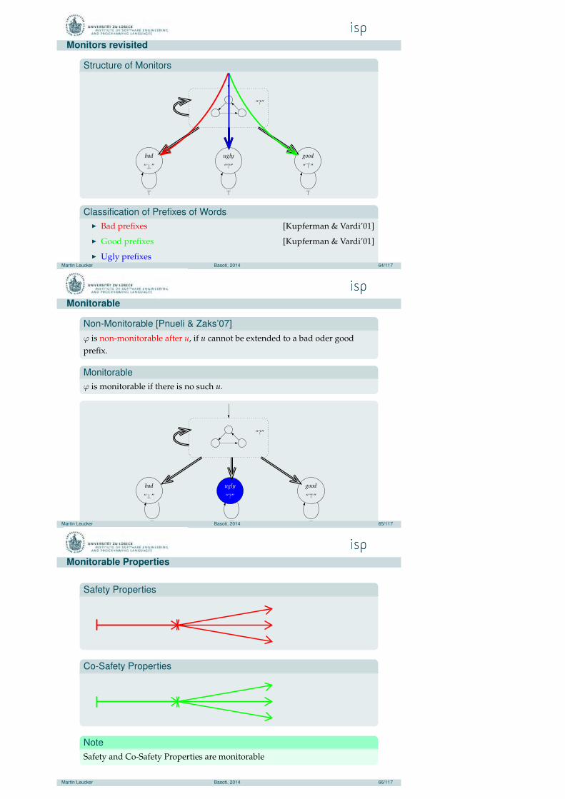
Monitors revisited
Structure of Monitors
“?”
bad
“⊥”
ugly
“?”
good
“⊤”
⊤ ⊤ ⊤
Classification of Prefixes of Words◮ Bad prefixes [Kupferman & Vardi’01]
◮ Good prefixes [Kupferman & Vardi’01]
◮ Ugly prefixesMartin Leucker Basoti, 2014 64/117
Monitorable
Non-Monitorable [Pnueli & Zaks’07]ϕ is non-monitorable after u, if u cannot be extended to a bad oder goodprefix.
Monitorableϕ is monitorable if there is no such u.
“?”
bad
“⊥”
ugly
“?”
good
“⊤”
⊤ ⊤ ⊤Martin Leucker Basoti, 2014 65/117
Monitorable Properties
Safety Properties
Co-Safety Properties
NoteSafety and Co-Safety Properties are monitorable
Martin Leucker Basoti, 2014 66/117
Safety- and Co-Safety-Properties
TheoremThe class of monitorable properties
◮ comprises safety- and co-safety properties, but
◮ is strictly larger than their union.
ProofConsider ((p ∨ q)Ur) ∨ Gp
Martin Leucker Basoti, 2014 67/117
Fusing model checking and runtime verification
LTL with a predictive semantics
Martin Leucker Basoti, 2014 69/117
Recall anticipatory LTL semantics
The truth value of a LTL3 formula ϕ wrt. u, denoted by [u |= ϕ], is an elementof B3 defined by
[u |= ϕ] =
⊤ if ∀σ ∈ Σω : uσ |= ϕ
⊥ if ∀σ ∈ Σω : uσ 6|= ϕ
? otherwise.
Martin Leucker Basoti, 2014 70/117
Applied to the empty word
Empty word ǫ
[ǫ |= ϕ]P = ⊤iff ∀σ ∈ Σω with ǫσ ∈ P : ǫσ |= ϕ
iff L(P) |= ϕ
RV more difficult than MC?Then runtime verification implicitly answers model checking
Martin Leucker Basoti, 2014 71/117
Abstraction
An over-abstraction or and over-approximation of a program P is a programP such that L(P) ⊆ L(P) ⊆ Σω .
Martin Leucker Basoti, 2014 72/117
Predictive Semantics
Definition (Predictive semantics of LTL)
Let P be a program and let P be an over-approximation of P . Let u ∈ Σ∗
denote a finite trace. The truth value of u and an LTL3 formula ϕ wrt. P ,denoted by [u |=P ϕ], is an element of B3 and defined as follows:
[u |=P ϕ] =
⊤ if ∀σ ∈ Σω with uσ ∈ P : uσ |= ϕ
⊥ if ∀σ ∈ Σω with uσ ∈ P : uσ 6|= ϕ
? else
We write LTLP whenever we consider LTL formulas with a predictivesemantics.
Martin Leucker Basoti, 2014 73/117
Properties of Predictive Semantics
Let P be an over-approximation of a program P over Σ, u ∈ Σ∗, andϕ ∈ LTL.
◮ Model checking is more precise than RV with the predictive semantics:
P |= ϕ implies [u |=P ϕ] ∈ {⊤, ?}
◮ RV has no false negatives: [u |=P ϕ] = ⊥ implies P 6|= ϕ
◮ The predictive semantics of an LTL formula is more precise than LTL3:
[u |= ϕ] = ⊤ implies [u |=P ϕ] = ⊤[u |= ϕ] = ⊥ implies [u |=P ϕ] = ⊥
The reverse directions are in general not true.
Martin Leucker Basoti, 2014 74/117
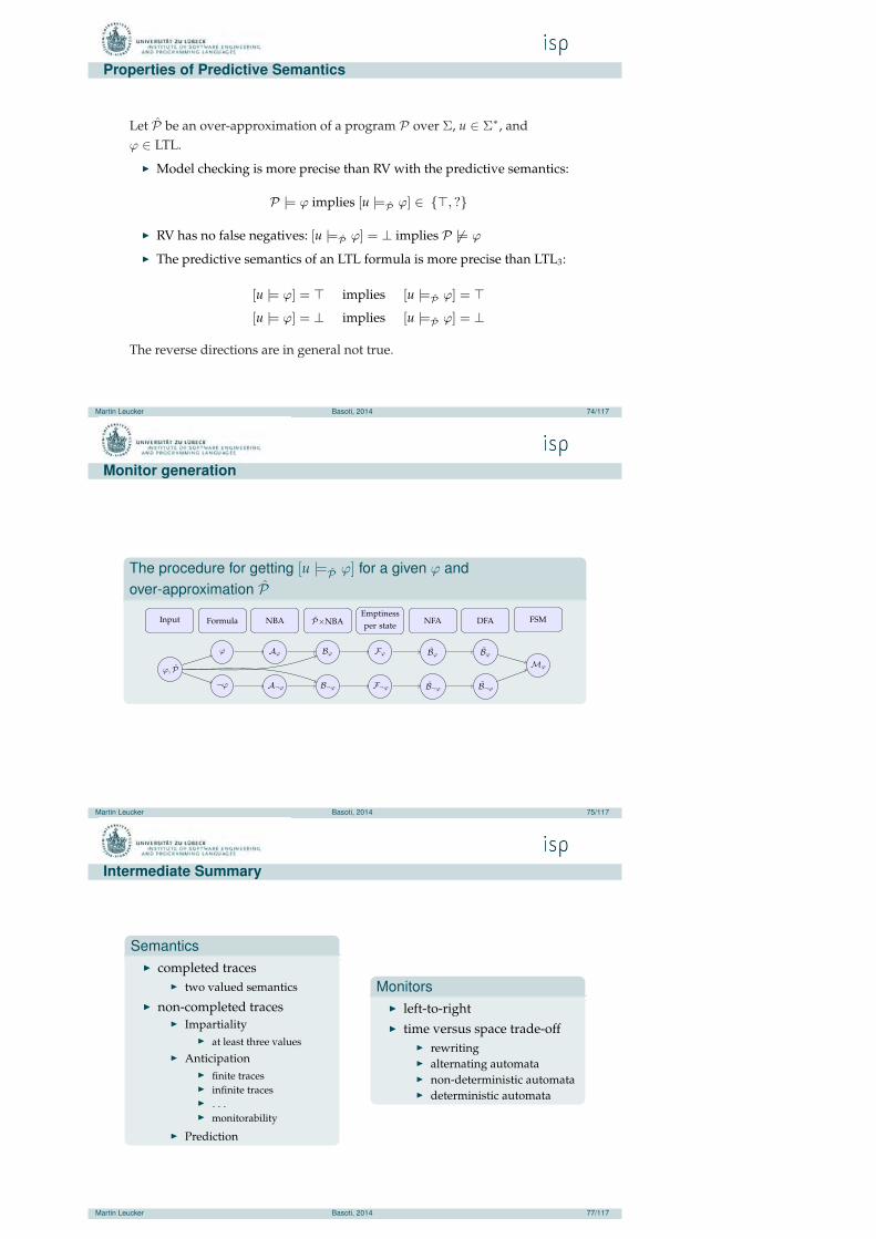
Monitor generation
The procedure for getting [u |=P ϕ] for a given ϕ andover-approximation P
ϕ, P
ϕ Aϕ Bϕ Fϕ Bϕ Bϕ
¬ϕ A¬ϕ B¬ϕ F¬ϕ B¬ϕ B¬ϕ
Mϕ
Input Formula NBA P×NBAEmptinessper state NFA DFA FSM
Martin Leucker Basoti, 2014 75/117
Intermediate Summary
Semantics◮ completed traces
◮ two valued semantics
◮ non-completed traces◮ Impartiality
◮ at least three values◮ Anticipation
◮ finite traces◮ infinite traces◮ . . .◮ monitorability
◮ Prediction
Monitors◮ left-to-right◮ time versus space trade-off
◮ rewriting◮ alternating automata◮ non-deterministic automata◮ deterministic automata
Martin Leucker Basoti, 2014 77/117
Presentation outlineRuntime VerificationRuntime Verification for LTL
LTL over Finite, Completed WordsLTL over Finite, Non-Completed Words: ImpartialityLTL over Non-Completed Words: AnticipationLTL over Infinite Words: With AnticipationGeneralisations: LTL with modulo ConstraintsMonitorable PropertiesLTL with a Predictive SemanticsLTL wrap-up
ExtensionsTesting Temporal Properties with RV: jUnitRVMonitoring Systems/LoggingSteeringDiagnosis
IdeasRV and Diagnosis
ConclusionMartin Leucker Basoti, 2014 78/117
Extensions
LTL is just half of the story
Martin Leucker Basoti, 2014 79/117
Extensions
LTL with data◮ J-LO
◮ MOP (parameterized LTL)
◮ RV for LTL with integer constraints
Further “rich” approaches◮ LOLA
◮ Eagle (etc.)
Further dimensions◮ real-time
◮ concurrency
◮ distribution
Martin Leucker Basoti, 2014 80/117
Presentation outlineRuntime VerificationRuntime Verification for LTL
LTL over Finite, Completed WordsLTL over Finite, Non-Completed Words: ImpartialityLTL over Non-Completed Words: AnticipationLTL over Infinite Words: With AnticipationGeneralisations: LTL with modulo ConstraintsMonitorable PropertiesLTL with a Predictive SemanticsLTL wrap-up
ExtensionsTesting Temporal Properties with RV: jUnitRVMonitoring Systems/LoggingSteeringDiagnosis
IdeasRV and Diagnosis
ConclusionMartin Leucker Basoti, 2014 81/117
Example Application
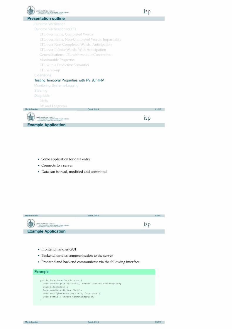
◮ Some application for data entry
◮ Connects to a server
◮ Data can be read, modified and committed
Martin Leucker Basoti, 2014 82/117
Example Application
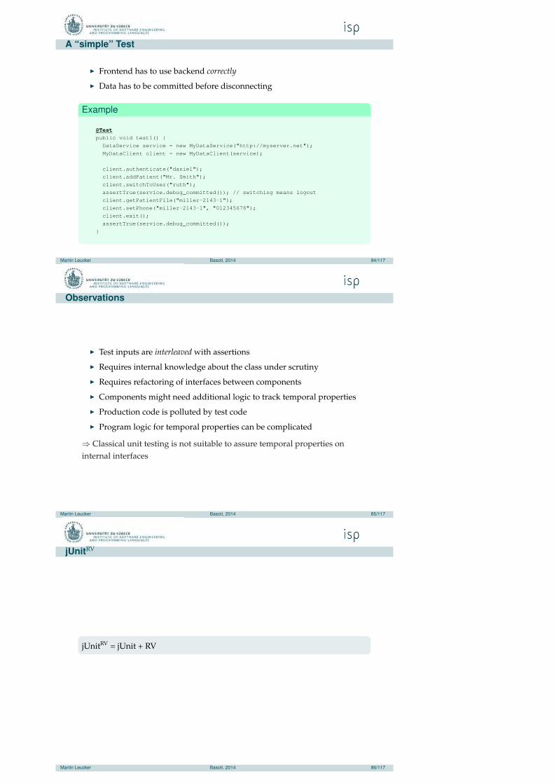
◮ Frontend handles GUI
◮ Backend handles communication to the server
◮ Frontend and backend communicate via the following interface:
Example
public interface DataService {
void connect(String userID) throws UnknownUserException;
void disconnect();
Data readData(String field);
void modifyData(String field, Data data);
void commit() throws CommitException;
}
Martin Leucker Basoti, 2014 83/117
A “simple” Test
◮ Frontend has to use backend correctly
◮ Data has to be committed before disconnecting
Example
@Testpublic void test1() {
DataService service = new MyDataService("http://myserver.net");
MyDataClient client = new MyDataClient(service);
client.authenticate("daniel");
client.addPatient("Mr. Smith");
client.switchToUser("ruth");
assertTrue(service.debug_committed()); // switching means logout
client.getPatientFile("miller-2143-1");
client.setPhone("miller-2143-1", "012345678");
client.exit();
assertTrue(service.debug_committed());
}
Martin Leucker Basoti, 2014 84/117
Observations
◮ Test inputs are interleaved with assertions
◮ Requires internal knowledge about the class under scrutiny
◮ Requires refactoring of interfaces between components
◮ Components might need additional logic to track temporal properties
◮ Production code is polluted by test code
◮ Program logic for temporal properties can be complicated
⇒ Classical unit testing is not suitable to assure temporal properties oninternal interfaces
Martin Leucker Basoti, 2014 85/117
jUnitRV
jUnitRV = jUnit + RV
Martin Leucker Basoti, 2014 86/117
Events and Propositions
◮ Formal runs consist of discrete steps in time
◮ When does a program perform a step?
◮ Explicitly specify events triggering time steps
◮ Only one event occurs at a point of time
◮ Propositions may be evaluated in the current state
Martin Leucker Basoti, 2014 87/117
Events and Propositions
Example (Specifying Events)
String dataService = "myPackage.DataService";
private static Event modify = called(dataService, "modify");
private static Event committed = returned(dataService, "commit");
private static Event disconnect = called(dataService, "disconnect");
Example (Specifying Propositions)
private static Proposition auth
= new Proposition(eq(invoke($this, "getStatus"),AUTH);
Martin Leucker Basoti, 2014 88/117
Temporal Assertion
◮ LTL is used to specify temporal properties
◮ Generated monitors only observe the specified events
◮ G(modify =⇒ ¬disconnectUcommitted)
Example (Specifying Monitors)
private static Monitor commitBeforeDisconnect = new FLTL4Monitor(
Always(implies(modify,
Until(not(disconnect), committed)
)
));
Martin Leucker Basoti, 2014 89/117
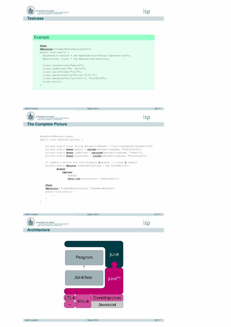
Testcase
Example
@Test@Monitors({"commitBeforeDisconnect"})public void test1() {
DataService service = new MyDataService("http://myserver.net");
MyDataClient client = new MyDataClient(service);
client.authenticate("daniel");
client.addPatient("Mr. Smith");
client.switchToUser("ruth");
client.getPatientFile("miller-2143-1");
client.setPhone("miller-2143-1", "012345678");
client.exit();
}
Martin Leucker Basoti, 2014 90/117
The Complete Picture
@RunWith(RVRunner.class)
public class MyDataClientTest {
private static final String dataServiceQname = "junitrvexamples.DataService";
private static Event modify = called(dataServiceQname, "modifyData");
private static Event committed = returned(dataServiceQname, "commit");
private static Event disconnect = invoke(dataServiceQname, "disconnect");
// create a monitor for LTL4 property G(modify -> !close U commit)
private static Monitor commitBeforeClose = new FLTL4Monitor(
Always(implies(
modify,
Until(not(disconnect), committed))));
@Test@Monitors({"commitBeforeClose", "authWhenModify"})
public void test1() {
...
}
}
Martin Leucker Basoti, 2014 91/117
Architecture
�✁✂✄✁☎✆
✝✞✟✠✡☛☞✌✡
✍✞✟✠✡
✎✏✑✠✒✓✔☞✟✡✕✟✍☞✖✡✠✂✟
✝☎✔☎✌✌✠✌✡
✑☛✑✗
✘✘✘
Martin Leucker Basoti, 2014 92/117
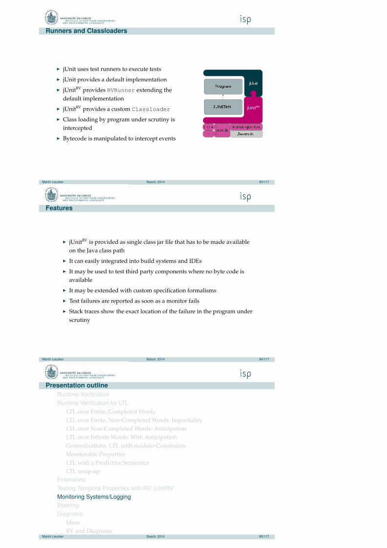
Runners and Classloaders
◮ jUnit uses test runners to execute tests
◮ jUnit provides a default implementation
◮ jUnitRV provides RVRunner extending thedefault implementation
◮ jUnitRV provides a custom Classloader
◮ Class loading by program under scrutiny isintercepted
◮ Bytecode is manipulated to intercept events
�✁✂✄✁☎✆
✝✞✟✠✡☛☞✌✡
✍✞✟✠✡
✎✏✑✠✒✓✔☞✟✡✕✟✍☞✖✡✠✂✟
✝☎✔☎✌✌✠✌✡
✑☛✑✗
✘✘✘
Martin Leucker Basoti, 2014 93/117
Features
◮ jUnitRV is provided as single class jar file that has to be made availableon the Java class path
◮ It can easily integrated into build systems and IDEs
◮ It may be used to test third party components where no byte code isavailable
◮ It may be extended with custom specification formalisms
◮ Test failures are reported as soon as a monitor fails
◮ Stack traces show the exact location of the failure in the program underscrutiny
Martin Leucker Basoti, 2014 94/117
Presentation outlineRuntime VerificationRuntime Verification for LTL
LTL over Finite, Completed WordsLTL over Finite, Non-Completed Words: ImpartialityLTL over Non-Completed Words: AnticipationLTL over Infinite Words: With AnticipationGeneralisations: LTL with modulo ConstraintsMonitorable PropertiesLTL with a Predictive SemanticsLTL wrap-up
ExtensionsTesting Temporal Properties with RV: jUnitRVMonitoring Systems/LoggingSteeringDiagnosis
IdeasRV and Diagnosis
ConclusionMartin Leucker Basoti, 2014 95/117

Monitoring Systems/Logging: Overview
monitoring systems/logging
instru-mentation
source code
byte code
binary code
logging APIs
trace tools
dedicatedtracing/-
monitoringhardware
Martin Leucker Basoti, 2014 96/117
Presentation outlineRuntime VerificationRuntime Verification for LTL
LTL over Finite, Completed WordsLTL over Finite, Non-Completed Words: ImpartialityLTL over Non-Completed Words: AnticipationLTL over Infinite Words: With AnticipationGeneralisations: LTL with modulo ConstraintsMonitorable PropertiesLTL with a Predictive SemanticsLTL wrap-up
ExtensionsTesting Temporal Properties with RV: jUnitRVMonitoring Systems/LoggingSteeringDiagnosis
IdeasRV and Diagnosis
ConclusionMartin Leucker Basoti, 2014 97/117
Monitoring Systems/Logging: Overview
monitoring results/steering
exception
steer
manual
automatically
Martin Leucker Basoti, 2014 98/117
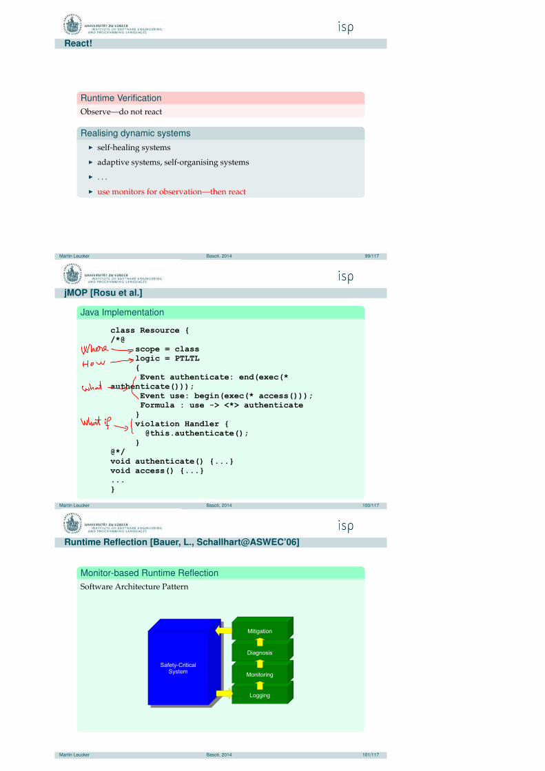
React!
Runtime VerificationObserve—do not react
Realising dynamic systems◮ self-healing systems
◮ adaptive systems, self-organising systems
◮ . . .
◮ use monitors for observation—then react
Martin Leucker Basoti, 2014 99/117
jMOP [Rosu et al.]
Java Implementation
Martin Leucker Basoti, 2014 100/117
Runtime Reflection [Bauer, L., Schallhart@ASWEC’06]
Monitor-based Runtime ReflectionSoftware Architecture Pattern
Martin Leucker Basoti, 2014 101/117
Presentation outlineRuntime VerificationRuntime Verification for LTL
LTL over Finite, Completed WordsLTL over Finite, Non-Completed Words: ImpartialityLTL over Non-Completed Words: AnticipationLTL over Infinite Words: With AnticipationGeneralisations: LTL with modulo ConstraintsMonitorable PropertiesLTL with a Predictive SemanticsLTL wrap-up
ExtensionsTesting Temporal Properties with RV: jUnitRVMonitoring Systems/LoggingSteeringDiagnosis
IdeasRV and Diagnosis
ConclusionMartin Leucker Basoti, 2014 102/117
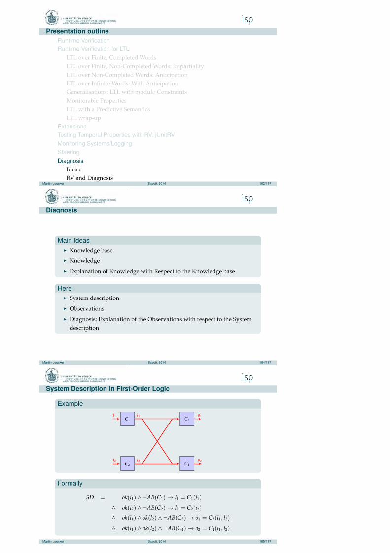
Diagnosis
Main Ideas◮ Knowledge base
◮ Knowledge
◮ Explanation of Knowledge with Respect to the Knowledge base
Here◮ System description
◮ Observations
◮ Diagnosis: Explanation of the Observations with respect to the Systemdescription
Martin Leucker Basoti, 2014 104/117
System Description in First-Order Logic
Example
C1
C2
C3
C4
i1 l1 o1
i2 l2 o2
Formally
SD = ok(i1) ∧ ¬AB(C1) → l1 = C1(i1)
∧ ok(i2) ∧ ¬AB(C2) → l2 = C2(i2)
∧ ok(l1) ∧ ok(l2) ∧ ¬AB(C3) → o1 = C3(l1, l2)
∧ ok(l1) ∧ ok(l2) ∧ ¬AB(C4) → o2 = C4(l1, l2)
Martin Leucker Basoti, 2014 105/117
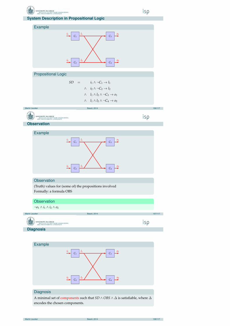
System Description in Propositional Logic
Example
C1
C2
C3
C4
i1 l1 o1
i2 l2 o2
Propositional Logic
SD = i1 ∧ ¬C1 → l1
∧ i2 ∧ ¬C2 → l2
∧ l1 ∧ l2 ∧ ¬C3 → o1
∧ l1 ∧ l2 ∧ ¬C4 → o2
Martin Leucker Basoti, 2014 106/117
Observation
Example
C1
C2
C3
C4
i1 l1 o1
i2 l2 o2
Observation(Truth) values for (some of) the propositions involvedFormally: a formula OBS
Observation¬o1 ∧ i1 ∧ i2 ∧ o2
Martin Leucker Basoti, 2014 107/117
Diagnosis
Example
C1
C2
C3
C4
i1 l1 o1
i2 l2 o2
DiagnosisA minimal set of components such that SD ∧ OBS ∧∆ is satisfiable, where ∆
encodes the chosen components.
Martin Leucker Basoti, 2014 108/117
Example
Example
C1
C2
C3
C4
i1 l1 o1
i2 l2 o2
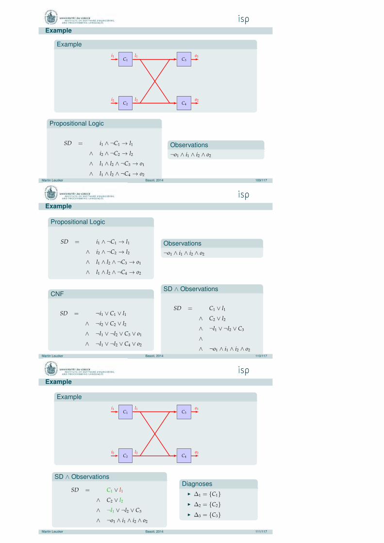
Propositional Logic
SD = i1 ∧ ¬C1 → l1
∧ i2 ∧ ¬C2 → l2
∧ l1 ∧ l2 ∧ ¬C3 → o1
∧ l1 ∧ l2 ∧ ¬C4 → o2
Observations¬o1 ∧ i1 ∧ i2 ∧ o2
Martin Leucker Basoti, 2014 109/117
Example
Propositional Logic
SD = i1 ∧ ¬C1 → l1
∧ i2 ∧ ¬C2 → l2
∧ l1 ∧ l2 ∧ ¬C3 → o1
∧ l1 ∧ l2 ∧ ¬C4 → o2
Observations¬o1 ∧ i1 ∧ i2 ∧ o2
CNF
SD = ¬i1 ∨ C1 ∨ l1
∧ ¬i2 ∨ C2 ∨ l2
∧ ¬l1 ∨ ¬l2 ∨ C3 ∨ o1
∧ ¬l1 ∨ ¬l2 ∨ C4 ∨ o2
SD ∧ Observations
SD = C1 ∨ l1
∧ C2 ∨ l2
∧ ¬l1 ∨ ¬l2 ∨ C3
∧∧ ¬o1 ∧ i1 ∧ i2 ∧ o2
Martin Leucker Basoti, 2014 110/117
Example
Example
C1
C2
C3
C4
i1 l1 o1
i2 l2 o2
SD ∧ Observations
SD = C1 ∨ l1
∧ C2 ∨ l2
∧ ¬l1 ∨ ¬l2 ∨ C3
∧ ¬o1 ∧ i1 ∧ i2 ∧ o2
Diagnoses◮ ∆1 = {C1}◮ ∆2 = {C2}◮ ∆3 = {C3}
Martin Leucker Basoti, 2014 111/117
Monitors yield Obervations
We have. . .◮ Monitor reports ⊥ line is false
◮ Monitor reports ? line is ? (no assignment)
◮ Monitor reports ⊤ line is ? (no assignment)
Omniscent MonitorsA monitor is called omnicscent if its output ⊤ implies that the results on themonitored output are indeed correct.
For Omniscent Monitors◮ Monitor reports ⊥ line is false
◮ Monitor reports ? line is ? (no assignment)
◮ Monitor reports ⊤ line is true
Martin Leucker Basoti, 2014 113/117
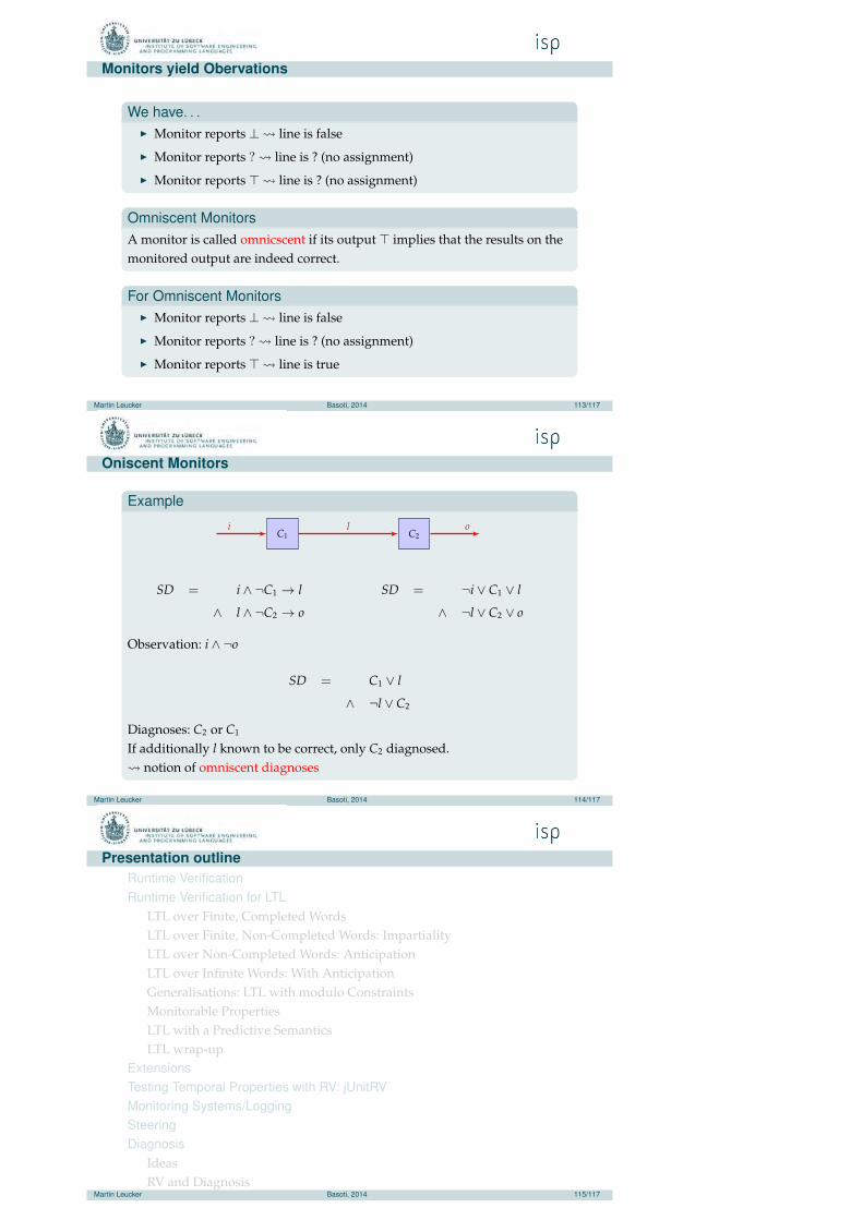
Oniscent Monitors
Example
C1 C2i l o
SD = i ∧ ¬C1 → l
∧ l ∧ ¬C2 → o
SD = ¬i ∨ C1 ∨ l
∧ ¬l ∨ C2 ∨ o
Observation: i ∧ ¬o
SD = C1 ∨ l
∧ ¬l ∨ C2
Diagnoses: C2 or C1
If additionally l known to be correct, only C2 diagnosed. notion of omniscent diagnoses
Martin Leucker Basoti, 2014 114/117
Presentation outlineRuntime VerificationRuntime Verification for LTL
LTL over Finite, Completed WordsLTL over Finite, Non-Completed Words: ImpartialityLTL over Non-Completed Words: AnticipationLTL over Infinite Words: With AnticipationGeneralisations: LTL with modulo ConstraintsMonitorable PropertiesLTL with a Predictive SemanticsLTL wrap-up
ExtensionsTesting Temporal Properties with RV: jUnitRVMonitoring Systems/LoggingSteeringDiagnosis
IdeasRV and Diagnosis
ConclusionMartin Leucker Basoti, 2014 115/117
Conclusion
Summary◮ RV for Failure detection
◮ various, multi-valued approaches◮ various existing systems◮ does generally identifies failure detection and identification
◮ Diagonis for Failure identification?
Future workWhat is the right combination?
Martin Leucker Basoti, 2014 116/117
That’s it!
Thanks! - Comments?
Martin Leucker Basoti, 2014 117/117


![Nonlinear System Identication in Structural Dynamics ......Nonlinear system identication is an integral part of the verication and validation (V&V) process. According to [21] , verication](https://img.pdfslide.us/doc/110x75/60e7c28aabdd680438454d71/nonlinear-system-identication-in-structural-dynamics-nonlinear-system-identication.jpg)