Software for a X Ray Tomograph

Rosario Martınez Gomez, Israel Vite Silva, and Luis G. de la Fraga

Cinvestav, Department of Computing.Av. Instituto Politecnico Nacional 2508. 07360 Mexico D.F., Mexico

Phone (+52) 55 50613755, E-mail: fraga@cs.cinvestav.mx

Abstract A software tool-box has been developed, which allows, notonly the volume reconstruction from X ray tomography images, but alsothe visualization of reconstructed isosurfaces. Although it may be con-sidered that the software needed is tightly linked to the hardware, we’llprove that we need five different (hardware independent) software com-ponents for the whole process: (1) acquisition, (2) projection’s centering,(3) reconstruction, (4) isosurfaces segmentation and (5) visualization.The reconstruction component was taken from Xmipp, an old softwarefor 3D reconstruction of biological macromolecules, segmentation wasdeveloped using k-means algorithm and the visualization was built usingthe splatting technique. In addition we compare splatting with anothertwo surface visualization techniques such as simple voxels and deformablesimplex meshes. The most of the software components were developedin C, C++ and perl. The graphical user interface for the visualizationcomponent was developed in C++ using Qt and OpenGL libraries.

Keywords: 3D visualization, splatting algorithm, tomography.

1 Introduction

The objective of a three-dimensional reconstruction is to obtain informationabout nature and structure of materials that conform the inside of an object.The are several applications, for example data from electron microscopes areused to reconstruct the molecular structure of proteins or to reconstruct the x-ray structure of an astronomical object such as supernova remnant, however oneof the most important applications has been in medicine to obtain the densitydistribution within the human body from multiple x-ray projections [1]. Thisprocess is referred to as computerized tomography and is a widely used technique,which enables the reconstruction from projections and the visualization of theinternal structure of objects.

A tomograph generates images, named projections, of cross sections of thescanned object, from data obtained by measuring the attenuation of x rays alonga large number of lines throughout specimen under study. Despite the fact thatacquisition part, in a process of computerized tomography, is tightly linked tothe hardware, another components of software are needed in order to solve the

whole problem of visualizing reconstructions. Thus, we have analyzed five mainparts of software:

1) projection’s acquisition, 2) projection’s centering, 3) specimen’s recon-struction, 4) segment the different densities of the reconstructed object, andthe last, 5) visualization of the surface for each segmented density. Every partis independent of the others and consists of one or several programs, but allparts must be used to resolve the whole problem of visualizing a tomographicreconstruction.

This paper is organized as follow: in section 2 are described part (1) to (4)of the developed software. In section 3 is described the visualization part devel-oped with splatting technique and it is compared with others two visualizationtechniques, one with voxels faces, and the other one with deformable simplexmeshes. Finally the conclusions are presented.

2 Software Parts

2.1 Acquisition

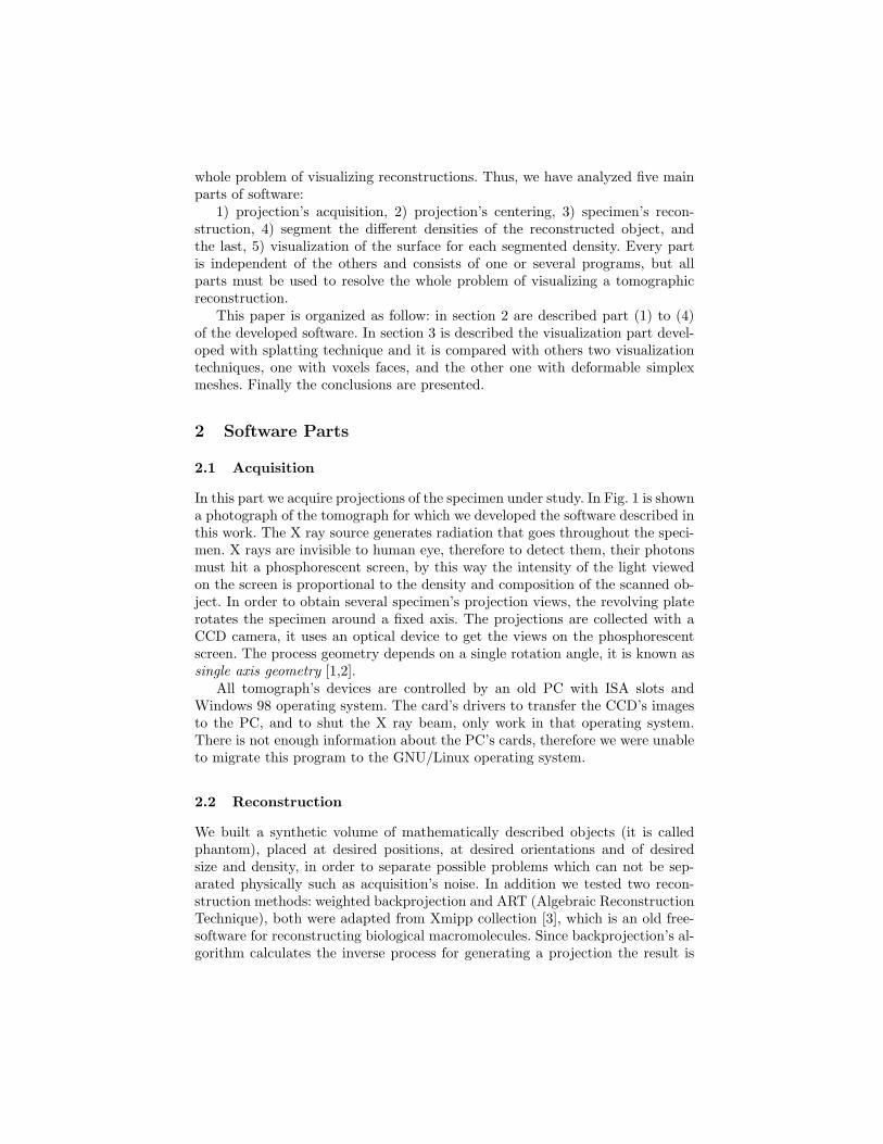
In this part we acquire projections of the specimen under study. In Fig. 1 is showna photograph of the tomograph for which we developed the software described inthis work. The X ray source generates radiation that goes throughout the speci-men. X rays are invisible to human eye, therefore to detect them, their photonsmust hit a phosphorescent screen, by this way the intensity of the light viewedon the screen is proportional to the density and composition of the scanned ob-ject. In order to obtain several specimen’s projection views, the revolving platerotates the specimen around a fixed axis. The projections are collected with aCCD camera, it uses an optical device to get the views on the phosphorescentscreen. The process geometry depends on a single rotation angle, it is known assingle axis geometry [1,2].

All tomograph’s devices are controlled by an old PC with ISA slots andWindows 98 operating system. The card’s drivers to transfer the CCD’s imagesto the PC, and to shut the X ray beam, only work in that operating system.There is not enough information about the PC’s cards, therefore we were unableto migrate this program to the GNU/Linux operating system.

2.2 Reconstruction

We built a synthetic volume of mathematically described objects (it is calledphantom), placed at desired positions, at desired orientations and of desiredsize and density, in order to separate possible problems which can not be sep-arated physically such as acquisition’s noise. In addition we tested two recon-struction methods: weighted backprojection and ART (Algebraic ReconstructionTechnique), both were adapted from Xmipp collection [3], which is an old free-software for reconstructing biological macromolecules. Since backprojection’s al-gorithm calculates the inverse process for generating a projection the result is

Figure 1: A tomograph’s photograph.

blurred, because the most of information is concentrated in the low frequen-cies. Then a filter must be applied to correct this problem. We implementedthe Wiener and Ramp filters and these are applied to each projection in thereciprocal space. Ramp-filter is typically used in weighted backprojection henceit produces more weight to high frequencies. On the other hand, Wiener-filterhas the aim of filtering noise which it is tightly linked to the acquisition process.

Ramp-filter is very simple, in two dimensions it is specified as in Eq. 1. Wherer is equal to the circle’s radius i.e.

√x2 + y2, and k is a constant proportional

to the Nyquist frequency [4].Although the reconstruction weighted by Ramp-filter is acceptable, it become

worse when noise is present since this filter amplifies high frequencies. In orderto solve it Wiener-filter could be used.

q(r) ={ |r|, if r ≤ k

0, if r > k(1)

To design the Wiener-filter, we require knowledge about noise and objectstatistics. Eq. 2 express the Wiener-filter, where f =

√(x2 + y2), and typical

used values are α = 0.5 and SNR = 60; the noise commonly is modeled as whiteadditive noise [5].

A(f, θ) =|f |2πα(SNR)

2πα(SNR) + |f |(α2 + 4π2f2)32

(2)

To test the developed programs we generated seventy two phantom’s pro-jections (taken every 5 degrees on the tilt angle), then we performed threereconstructions using the reconstruction algorithms: backprojection, weightedbackprojection, and ART. To compare the reconstructions, we drew the changesin the density along the 15th row on the 30th slice as is shown in Fig. ref-fig:eficiencia. The simple line represents the values of the original phantom’sdensities, the backprojection-reconstruction is represented by the square-line, it

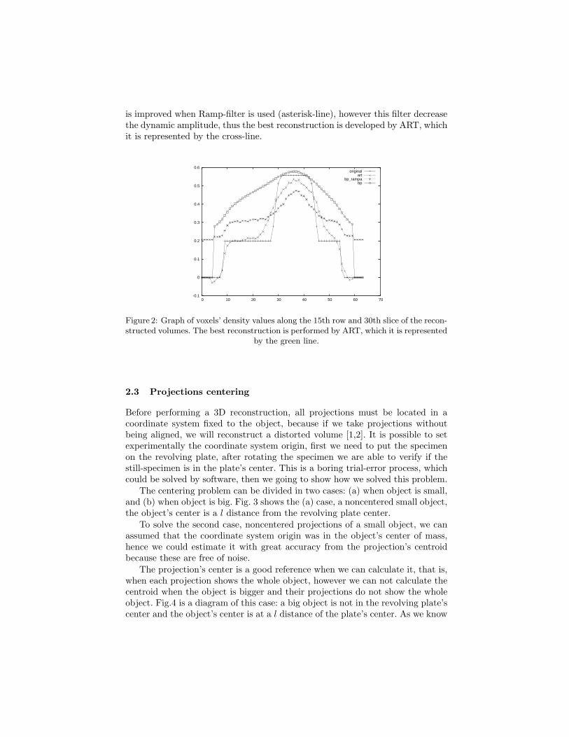
is improved when Ramp-filter is used (asterisk-line), however this filter decreasethe dynamic amplitude, thus the best reconstruction is developed by ART, whichit is represented by the cross-line.

-0.1

0

0.1

0.2

0.3

0.4

0.5

0.6

0 10 20 30 40 50 60 70

originalart

bp_rampabp

Figure 2: Graph of voxels’ density values along the 15th row and 30th slice of the recon-structed volumes. The best reconstruction is performed by ART, which it is represented

by the green line.

2.3 Projections centering

Before performing a 3D reconstruction, all projections must be located in acoordinate system fixed to the object, because if we take projections withoutbeing aligned, we will reconstruct a distorted volume [1,2]. It is possible to setexperimentally the coordinate system origin, first we need to put the specimenon the revolving plate, after rotating the specimen we are able to verify if thestill-specimen is in the plate’s center. This is a boring trial-error process, whichcould be solved by software, then we going to show how we solved this problem.

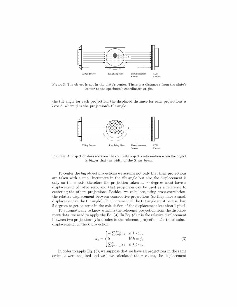
The centering problem can be divided in two cases: (a) when object is small,and (b) when object is big. Fig. 3 shows the (a) case, a noncentered small object,the object’s center is a l distance from the revolving plate center.

To solve the second case, noncentered projections of a small object, we canassumed that the coordinate system origin was in the object’s center of mass,hence we could estimate it with great accuracy from the projection’s centroidbecause these are free of noise.

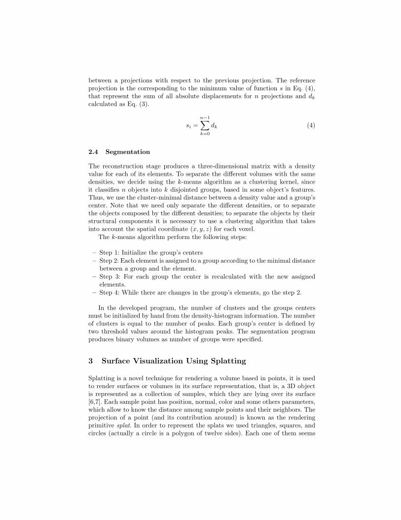
The projection’s center is a good reference when we can calculate it, that is,when each projection shows the whole object, however we can not calculate thecentroid when the object is bigger and their projections do not show the wholeobject. Fig.4 is a diagram of this case: a big object is not in the revolving plate’scenter and the object’s center is at a l distance of the plate’s center. As we know

PhosphorescentScreen

CCDCamera

l

X Ray Source Revolving Plate

Figure 3: The object is not in the plate’s center. There is a distance l from the plate’scenter to the specimen’s coordinates origin.

the tilt angle for each projection, the displaced distance for each projections isl cos φ, where φ is the projection’s tilt angle.

����������������������������

����������������������������

PhosphorescentScreen

CCDCamera

l

X Ray Source Revolving Plate

Figure 4: A projection does not show the complete object’s information when the objectis bigger that the width of the X ray beam.

To center the big object projections we assume not only that their projectionsare taken with a small increment in the tilt angle but also the displacement isonly on the x axis, therefore the projection taken at 90 degrees must have adisplacement of value zero, and that projection can be used as a reference tocentering the others projections. Besides, we calculate, using cross-correlation,the relative displacement between consecutive projections (so they have a smalldisplacement in the tilt angle). The increment in the tilt angle must be less than5 degrees to get an error in the calculation of the displacement less than 1 pixel.

To automatically to know which is the reference projection from the displace-ment data, we need to apply the Eq. (3). In Eq. (3) x is the relative displacementbetween two projections, j is a index to the reference projection, d is the absolutedisplacement for the k projection.

dk =

−∑j−1i=k xi if k < j,

0 if k = j,∑ki=j+1 xi if k > j,

(3)

In order to apply Eq. (3), we suppose that we have all projections in the sameorder as were acquired and we have calculated the x values, the displacement

between a projections with respect to the previous projection. The referenceprojection is the corresponding to the minimum value of function s in Eq. (4),that represent the sum of all absolute displacements for n projections and dk

calculated as Eq. (3).

si =n−1∑

k=0

dk (4)

2.4 Segmentation

The reconstruction stage produces a three-dimensional matrix with a densityvalue for each of its elements. To separate the different volumes with the samedensities, we decide using the k-means algorithm as a clustering kernel, sinceit classifies n objects into k disjointed groups, based in some object’s features.Thus, we use the cluster-minimal distance between a density value and a group’scenter. Note that we need only separate the different densities, or to separatethe objects composed by the different densities; to separate the objects by theirstructural components it is necessary to use a clustering algorithm that takesinto account the spatial coordinate (x, y, z) for each voxel.

The k-means algorithm perform the following steps:

– Step 1: Initialize the group’s centers– Step 2: Each element is assigned to a group according to the minimal distance

between a group and the element.– Step 3: For each group the center is recalculated with the new assigned

elements.– Step 4: While there are changes in the group’s elements, go the step 2.

In the developed program, the number of clusters and the groups centersmust be initialized by hand from the density-histogram information. The numberof clusters is equal to the number of peaks. Each group’s center is defined bytwo threshold values around the histogram peaks. The segmentation programproduces binary volumes as number of groups were specified.

3 Surface Visualization Using Splatting

Splatting is a novel technique for rendering a volume based in points, it is usedto render surfaces or volumes in its surface representation, that is, a 3D objectis represented as a collection of samples, which they are lying over its surface[6,7]. Each sample point has position, normal, color and some others parameters,which allow to know the distance among sample points and their neighbors. Theprojection of a point (and its contribution around) is known as the renderingprimitive splat. In order to represent the splats we used triangles, squares, andcircles (actually a circle is a polygon of twelve sides). Each one of them seems

a small planar patch, which are assigned to a point oriented along the object’ssurface.

The aim of our software component is to visualize the surface of the recon-structed volumes using the splatting technique. So as to perform this part thefollowing steps were made:

– Step 1: Extract the surface for each segmented volume using mathematicalmorphology. The center of each voxel will be the coordinates of the point andthis point will be used to represent the surface.

– Step 2: Calculate the normal to each point over the surface.

– Step 3: Associate a splat to each surface point and set its position according withits normal.

By subtracting an eroded volume (it built with a structural element whichconsists of a voxel and its six neighbors), to the original volume we performedstep 1, the extraction of the voxels in the binary volume surface; so that wedeveloped an program which receives a binary volume and produces anotherbinary volume only with the surface voxels set to 1.

The step 2 is solved in very simple way: A plane is fitted to a point andits neighborhood, then the point’s normal is obtained. The plane’s equation isgiven by Ax + By + Cz + D = 0, in addition if we divide this equation by D,we will obtain A′x + B′y + C ′z = −1, that is, we only need three points forobtaining the values of the three unknowns, however we could have 27 points inthe neighborhood; therefore we decide to use the SVD method (Singular ValueDecomposition) to solve the overdetermined system, moreover by using SVD weassure that we have gotten the best plane fitted in the least squares sense. Oncewe calculated the plane we know that the point’s normal is (A,B, C). Now weneed the correct normal direction, so we checked the values of the two neighborsvoxels in the normal’s position of the original volume; the correct direction iswhere the neighbor voxel has the value of 0 (outside the volume no densityexists).

Finally, to perform the step 3, a splat is represented using OpenGL-primitives;for that reason we designed and programed an graphical user interface (GUI)made in Qt [8] and OpenGL [9] to visualize the volumes. Qt is a library torapid prototyping developed in C++, it has an excellent documentation, and itallows to assign an OpenGL-widget to the GUI. As input to the GUI we havea file with the format: a number in a single row that represents the maximumdistance between two voxels, 6 numbers per row of the three coordinates valuesto every point and three of their normal’s values. Coordinates-values must benormalized between −0.5 and 0.5. The splat-rendering primitive was performedwhen the visualization is made, that is, a splat is assigned to every point, locatedaccording to its normal, and with a size of the maximum distance of two voxelsin order to avoid holes in the visualization. Furthermore, we represented splatsas triangles, squares, and circles, besides it allows the visualization of points asa quick visualization help.

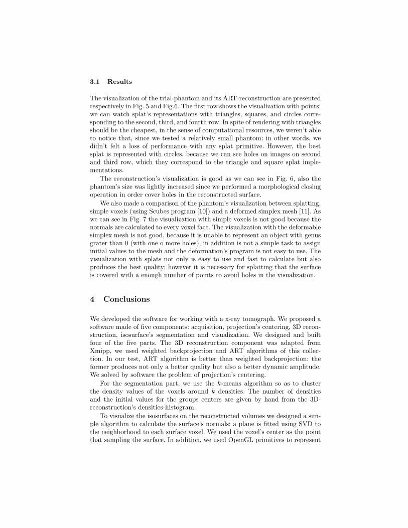
3.1 Results

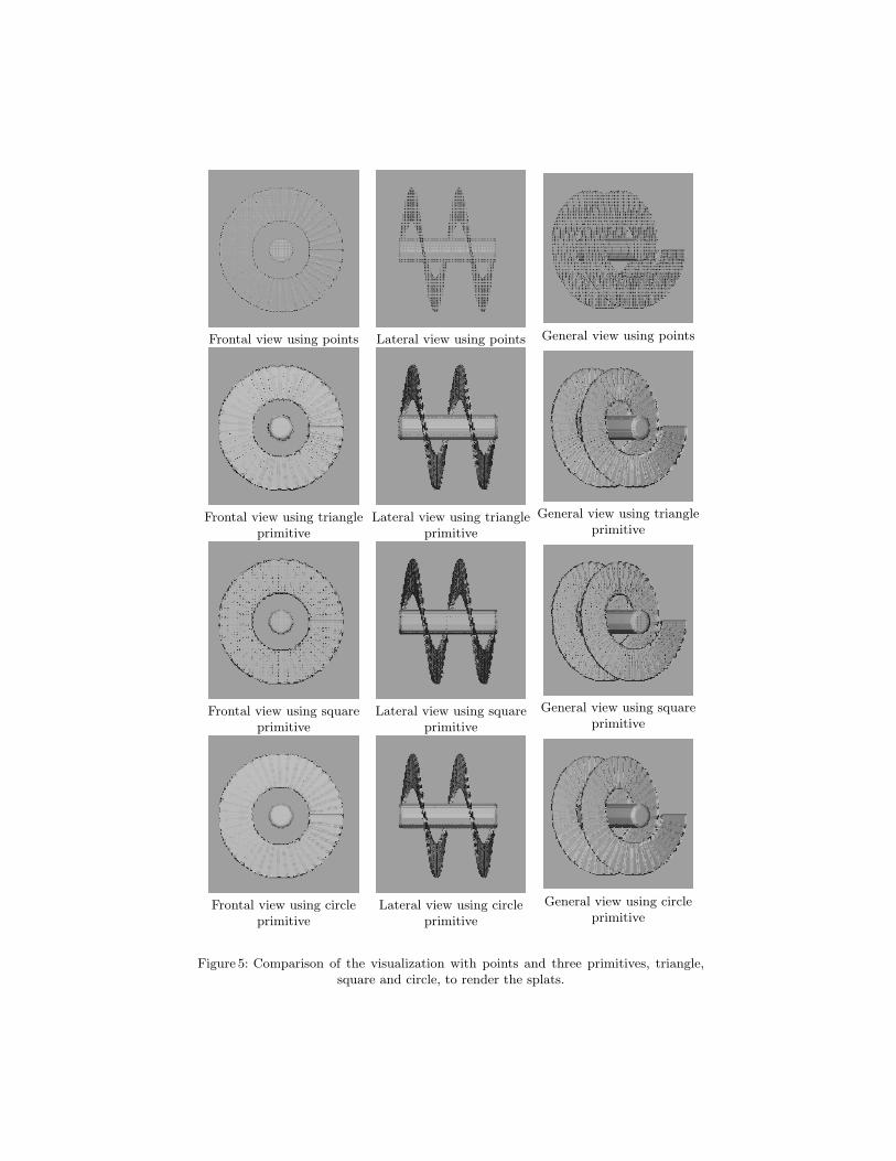
The visualization of the trial-phantom and its ART-reconstruction are presentedrespectively in Fig. 5 and Fig.6. The first row shows the visualization with points;we can watch splat’s representations with triangles, squares, and circles corre-sponding to the second, third, and fourth row. In spite of rendering with trianglesshould be the cheapest, in the sense of computational resources, we weren’t ableto notice that, since we tested a relatively small phantom; in other words, wedidn’t felt a loss of performance with any splat primitive. However, the bestsplat is represented with circles, because we can see holes on images on secondand third row, which they correspond to the triangle and square splat imple-mentations.

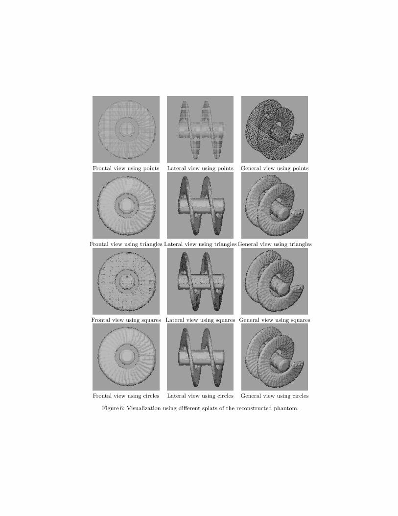
The reconstruction’s visualization is good as we can see in Fig. 6, also thephantom’s size was lightly increased since we performed a morphological closingoperation in order cover holes in the reconstructed surface.

We also made a comparison of the phantom’s visualization between splatting,simple voxels (using Scubes program [10]) and a deformed simplex mesh [11]. Aswe can see in Fig. 7 the visualization with simple voxels is not good because thenormals are calculated to every voxel face. The visualization with the deformablesimplex mesh is not good, because it is unable to represent an object with genusgrater than 0 (with one o more holes), in addition is not a simple task to assigninitial values to the mesh and the deformation’s program is not easy to use. Thevisualization with splats not only is easy to use and fast to calculate but alsoproduces the best quality; however it is necessary for splatting that the surfaceis covered with a enough number of points to avoid holes in the visualization.

4 Conclusions

We developed the software for working with a x-ray tomograph. We proposed asoftware made of five components: acquisition, projection’s centering, 3D recon-struction, isosurface’s segmentation and visualization. We designed and builtfour of the five parts. The 3D reconstruction component was adapted fromXmipp, we used weighted backprojection and ART algorithms of this collec-tion. In our test, ART algorithm is better than weighted backprojection: theformer produces not only a better quality but also a better dynamic amplitude.We solved by software the problem of projection’s centering.

For the segmentation part, we use the k-means algorithm so as to clusterthe density values of the voxels around k densities. The number of densitiesand the initial values for the groups centers are given by hand from the 3D-reconstruction’s densities-histogram.

To visualize the isosurfaces on the reconstructed volumes we designed a sim-ple algorithm to calculate the surface’s normals: a plane is fitted using SVD tothe neighborhood to each surface voxel. We used the voxel’s center as the pointthat sampling the surface. In addition, we used OpenGL primitives to represent

a splat, we tested the primitives of triangles, squares, and circles. The best visu-alization in provided by the circles (actually a circle is a polygon of twelve sides).We show that splatting is easy to use give us the best quality visualization.

We think that all the programs developed must be tunned according to aspecific application, therefore they must be changed to adjust the visualizationto an specific reconstruction application task.

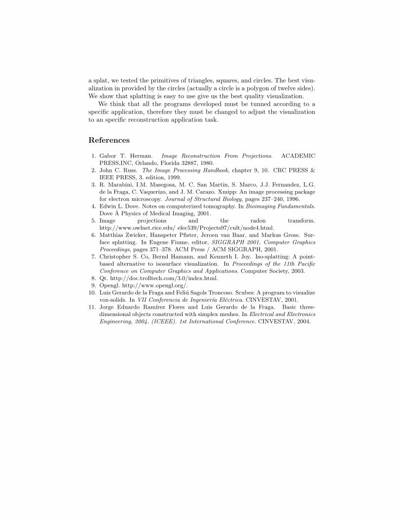
References

1. Gabor T. Herman. Image Reconstruction From Projections. ACADEMICPRESS,INC, Orlando, Florida 32887, 1980.

2. John C. Russ. The Image Processing Handbook, chapter 9, 10. CRC PRESS &IEEE PRESS, 3. edition, 1999.

3. R. Marabini, I.M. Masegosa, M. C. San Martin, S. Marco, J.J. Fernandez, L.G.de la Fraga, C. Vaquerizo, and J. M. Carazo. Xmipp: An image processing packagefor electron microscopy. Journal of Structural Biology, pages 237–240, 1996.

4. Edwin L. Dove. Notes on computerized tomography. In Bioimaging Fundamentals.Dove A Physics of Medical Imaging, 2001.

5. Image projections and the radon transform.http://www.owlnet.rice.edu/ elec539/Projects97/cult/node4.html.

6. Matthias Zwicker, Hanspeter Pfister, Jeroen van Baar, and Markus Gross. Sur-face splatting. In Eugene Fiume, editor, SIGGRAPH 2001, Computer GraphicsProceedings, pages 371–378. ACM Press / ACM SIGGRAPH, 2001.

7. Christopher S. Co, Bernd Hamann, and Kenneth I. Joy. Iso-splatting: A point-based alternative to isosurface visualization. In Proceedings of the 11th PacificConference on Computer Graphics and Applications. Computer Society, 2003.

8. Qt. http://doc.trolltech.com/3.0/index.html.9. Opengl. http://www.opengl.org/.

10. Luis Gerardo de la Fraga and Feliu Sagols Troncoso. Scubes: A program to visualizevox-solids. In VII Conferencia de Ingenierıa Electrica. CINVESTAV, 2001.

11. Jorge Eduardo Ramırez Flores and Luis Gerardo de la Fraga. Basic three-dimensional objects constructed with simplex meshes. In Electrical and ElectronicsEngineering, 2004. (ICEEE). 1st International Conference. CINVESTAV, 2004.

Frontal view using points Lateral view using points General view using points

Frontal view using triangleprimitive

Lateral view using triangleprimitive

General view using triangleprimitive

Frontal view using squareprimitive

Lateral view using squareprimitive

General view using squareprimitive

Frontal view using circleprimitive

Lateral view using circleprimitive

General view using circleprimitive

Figure 5: Comparison of the visualization with points and three primitives, triangle,square and circle, to render the splats.

Frontal view using points Lateral view using points General view using points

Frontal view using triangles Lateral view using trianglesGeneral view using triangles

Frontal view using squares Lateral view using squares General view using squares

Frontal view using circles Lateral view using circles General view using circles

Figure 6: Visualization using different splats of the reconstructed phantom.

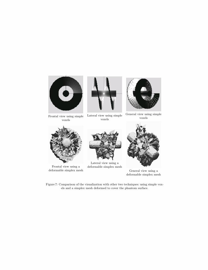
Frontal view using simplevoxels

Lateral view using simplevoxels

General view using simplevoxels

Frontal view using adeformable simplex mesh

Lateral view using adeformable simplex mesh

General view using adeformable simplex mesh

Figure 7: Comparison of the visualization with other two techniques: using simple vox-els and a simplex mesh deformed to cover the phantom surface.