Embed Size (px)
Citation preview
Forschungsinstitut zur Zukunft der ArbeitInstitute for the Study of Labor
DI
SC
US
SI
ON
P
AP
ER
S
ER
IE
S
Soda Taxes and the Prices of Sodas and Other Drinks:Evidence from Mexico
IZA DP No. 9682
January 2016
Jeffrey Grogger
Soda Taxes and the Prices of
Sodas and Other Drinks: Evidence from Mexico
Jeffrey Grogger University of Chicago
and IZA
Discussion Paper No. 9682 January 2016
IZA
P.O. Box 7240 53072 Bonn
Germany
Phone: +49-228-3894-0 Fax: +49-228-3894-180
E-mail: [email protected]
Any opinions expressed here are those of the author(s) and not those of IZA. Research published in this series may include views on policy, but the institute itself takes no institutional policy positions. The IZA research network is committed to the IZA Guiding Principles of Research Integrity. The Institute for the Study of Labor (IZA) in Bonn is a local and virtual international research center and a place of communication between science, politics and business. IZA is an independent nonprofit organization supported by Deutsche Post Foundation. The center is associated with the University of Bonn and offers a stimulating research environment through its international network, workshops and conferences, data service, project support, research visits and doctoral program. IZA engages in (i) original and internationally competitive research in all fields of labor economics, (ii) development of policy concepts, and (iii) dissemination of research results and concepts to the interested public. IZA Discussion Papers often represent preliminary work and are circulated to encourage discussion. Citation of such a paper should account for its provisional character. A revised version may be available directly from the author.
IZA Discussion Paper No. 9682 January 2016
ABSTRACT
Soda Taxes and the Prices of Sodas and Other Drinks: Evidence from Mexico*
To combat a growing obesity problem, Mexico imposed a nationwide tax on drinks with added sugar, popularly referred to as a “soda tax,” effective January 2014. Since the tax took effect nationwide, there is no conventional control group that can be used as a baseline to estimate how the tax affected prices. Instead, I make use of control commodities, that is, untaxed goods that are not substitutes for the taxed drinks. I analyze data from Mexico’s Consumer Price Index program, using the synthetic control method and a time-series intervention analysis. I employ a placebo inference approach, akin to permutation inference, in both cases. The estimates show that soda prices rose by more than the amount of the tax. There is less evidence that the prices of potential substitutes rose, possibly indicating that consumers did not switch to those products after the tax took effect. Some simple calculations suggest that the soda price increase could lead to a two- to four-pound reduction in mean weight. This in turn amounts to roughly 1.6 to 2.7 percent of mean body mass, which compares to weight reductions that analysts have argued would have meaningful health consequences in the U.S. JEL Classification: H22, I10 Keywords: soda taxes, overshifting, obesity Corresponding author: Jeffrey Grogger Chicago Harris School of Public Policy University of Chicago 1155 E. 60th Street Chicago, IL 60637 USA E-mail: [email protected]
* I thank Michael Fosco, Paul Li, Ursina Schaede, and Alex Warofka for excellent research assistance. I thank Alberto Abadie, Christian Hansen, and participants in the Becker Friedman Institute’s Becker Brown Bag series for comments. This paper is a substantial revision of an earlier working paper circulated under the same title. Any errors are the author’s.
I. Introduction
Obesity is a major health problem. It is strongly linked to diabetes, heart disease, and
other forms of chronic illness, which are leading causes of death in much of the world
(Malnick & Knobler, 2006; World Health Organzition, 2014). In the U.S., 69 percent of
adults are overweight, meaning that their body mass index (the ratio of weight in
kilograms to the square of height in meters) is over 25. Thirty-five percent are obese,
meaning their BMI is over 30 (Ogden, Carroll, Kit, & Flegal, 2014). Olshansky et al.
(2005) argue that recent obesity trends may reduce the life expectancy of future
generations of Americans.
Obesity is also a pressing problem elsewhere. Over three-fifths of the world’s obese
individuals live in low- or middle-income counties (Ng et al., 2014). In Mexico, 73
percent of adults are overweight and 33 percent are obese (Gutierrez, Rivera, Shamah,
Oropeza, & Avila, 2012). Analysts estimate that obesity-related disease accounted for 13
percent of Mexican health expenditures in 2008, and project that those costs will double
by 2017 (Martinez, Lopez-Espinoza, & Lopez-Uriarte, 2015).
Obesity has been linked to sugar consumption, particularly to the consumption of sodas
and other drinks with added sugar (Malik, Schulze, & Hu, 2006). Such beverages deliver
many calories without simultaneously reducing appetite. Thus consumers who drink
sugary beverages tend not to offset their calories by reducing their consumption of other
food or drink (DiMeglio & Mattes, 2000).
The link between sugary drinks and obesity has led many governments to impose taxes
on drinks with added sugar. The theory is simple: a tax should raise the price paid by
2
consumers, which in turn should reduce consumption. Beyond that, theory provides only
guidelines about the amount by which prices should rise. In a competitive market, price
should rise by no more than the tax. In monopoly markets, however, price may rise by
less than the tax, by the amount of the tax, or even by more than the tax, depending on the
shape of the demand curve. Models of intermediate market structure make a similarly
broad range of predictions (Anderson, Palma, & Kreider, 2001; Delipalla & Keen, 1992;
Hamilton, 2015; Stern, 1987). Since the health benefits of a soda tax depend strongly the
extent to which the tax discourages consumption, it is important to quantify how the tax
affects prices.
The health benefits of a soda tax also depend on consumers’ substitution patterns.
Reductions in soda consumption could have substantial effects on weight if consumers
substitute toward low-calorie beverages such as water. If instead they substitute toward
high-calorie beverages such as milk, weight may not fall much.
In this paper I analyze how Mexico’s so-called soda tax has affected the prices of both
taxed beverages and untaxed substitutes. The tax, which amounted to roughly nine
percent of the mean pre-tax price of sodas, was imposed beginning January 2014. It
covers not just sodas, but almost all drinks that contain added sugar. I estimate the
effects of the tax on the price of such drinks by tracking the change in prices across 46
Mexican cities.
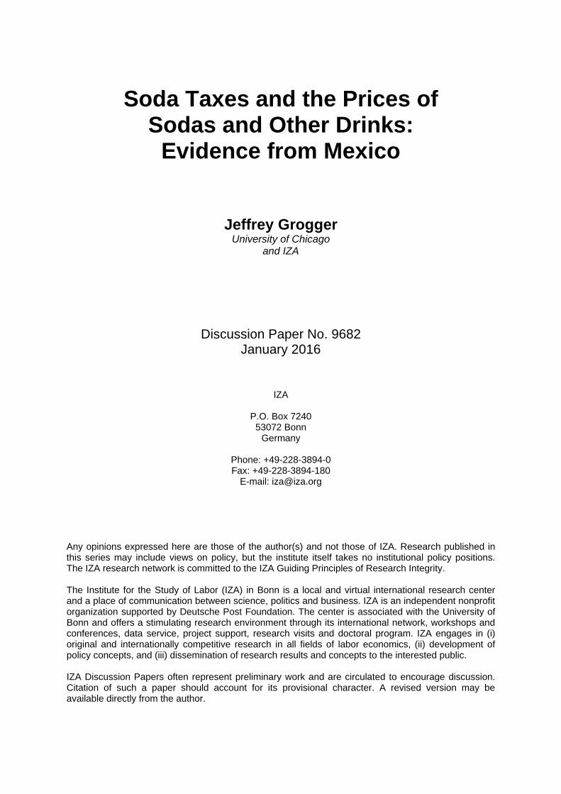
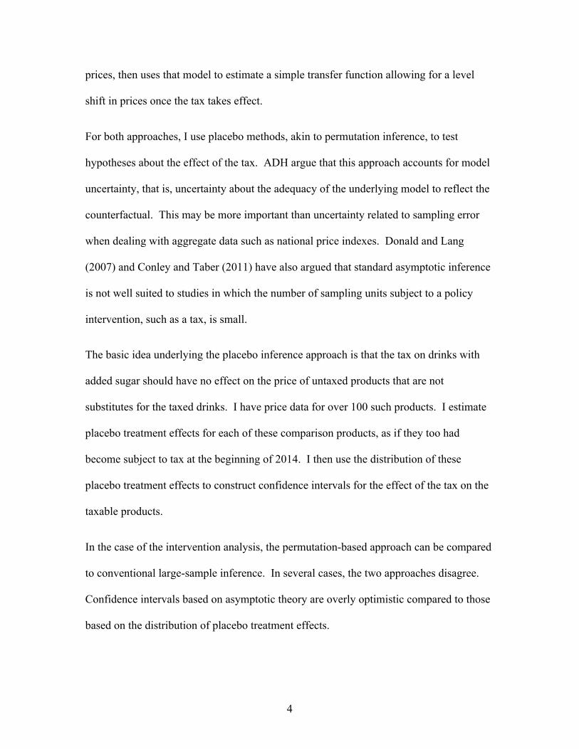
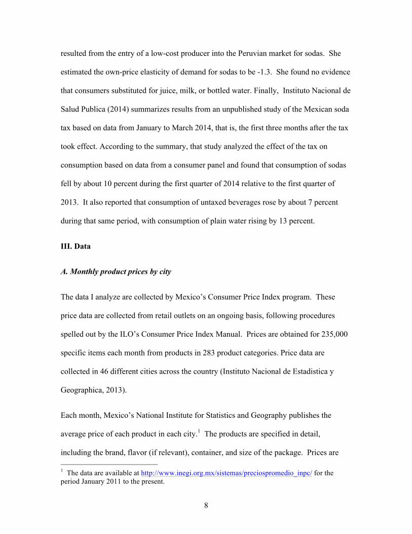
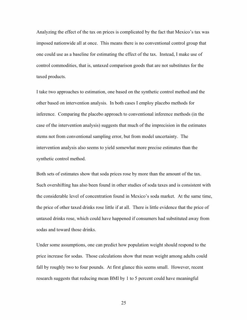
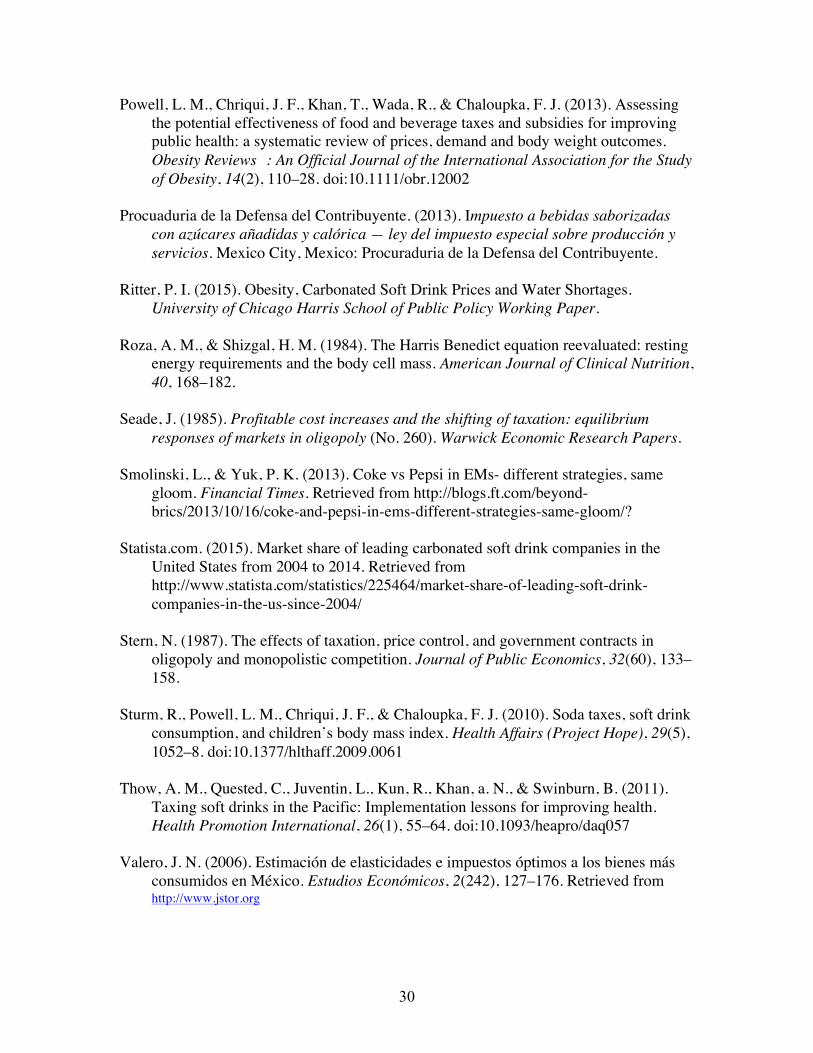
Figure 1 provides strongly suggestive evidence that the tax raised the price of sodas, an
important class of taxable drinks. It plots the Mexican Consumer Price Index (CPI) for

3
sodas (refrescos in Spanish) by month for the period January 2010 to March 2015. Prices
jumped sharply in January 2014, the month that the tax took effect.
I also analyze the prices of other drinks with added sugar, as well as the prices of
potential substitutes that are not subject to the tax, such as diet sodas, bottled water, pure
fruit juice, and milk. Basic economic theory predicts that if consumers substitute toward
these products as the price of taxed drinks rises, and the supply curve of untaxed drinks is
upward sloping, then the price of untaxed drinks should rise as well. Thus changes in the
price of untaxed substitutes may provide indirect evidence on consumer substitution
patterns.
A challenge for estimation is that the soda tax took effect at the same time nationwide. If
other economy-wide factors were putting pressure on prices in early 2014, then the
change in drink prices that I attribute to the tax may instead be the result of those other
factors. I take two approaches to deal with this problem. The first is to utilize the
synthetic control method of Abadie, Diamond, and Hainmueller (2010, hereafter ADH).
This approach constructs a synthetic control product based on pre-tax data and estimates
the effect of the tax from the post-tax difference between the soda price and the price of
the synthetic control product. The synthetic control product is selected as a convex
combination of a large number of untaxed comparison products so as to most closely
track the pre-tax path of soda prices.
The second approach is based on intervention analysis, also known as interrupted time-
series analysis, a technique first proposed by Box and Tiao (1975). This approach
proceeds in two steps. One first estimates an ARIMA model to pre-tax data on soda
4
prices, then uses that model to estimate a simple transfer function allowing for a level
shift in prices once the tax takes effect.
For both approaches, I use placebo methods, akin to permutation inference, to test
hypotheses about the effect of the tax. ADH argue that this approach accounts for model
uncertainty, that is, uncertainty about the adequacy of the underlying model to reflect the
counterfactual. This may be more important than uncertainty related to sampling error
when dealing with aggregate data such as national price indexes. Donald and Lang
(2007) and Conley and Taber (2011) have also argued that standard asymptotic inference
is not well suited to studies in which the number of sampling units subject to a policy
intervention, such as a tax, is small.
The basic idea underlying the placebo inference approach is that the tax on drinks with
added sugar should have no effect on the price of untaxed products that are not
substitutes for the taxed drinks. I have price data for over 100 such products. I estimate
placebo treatment effects for each of these comparison products, as if they too had
become subject to tax at the beginning of 2014. I then use the distribution of these
placebo treatment effects to construct confidence intervals for the effect of the tax on the
taxable products.
In the case of the intervention analysis, the permutation-based approach can be compared
to conventional large-sample inference. In several cases, the two approaches disagree.
Confidence intervals based on asymptotic theory are overly optimistic compared to those
based on the distribution of placebo treatment effects.
5
Finally, I provide some rough calculations designed to gauge the extent to which the soda
tax may contribute to weight loss. These are based on existing estimates of the elasticity
of demand for sodas in Mexico and standard formulas relating calorie intake to steady-
state weight changes. Not surprisingly, a nine-percent tax on sodas is not enough to
eliminate obesity. At the same time, the weight-loss calculations are comparable to
amounts that have been argued to have meaningful effects on health.
In the next section of the paper, I provide more information about Mexico’s soda tax and
about previous studies on the links between soda taxes, soda prices, and consumption. In
section III I discuss the data; Section IV takes up estimation and inference. Section V
presents results, Section VI translates the estimated price effects into effects on
consumption and weight, and Section VII concludes.
II. Background
A. Mexico’s tax on drinks with added sugar and its soft-drink market
Mexico’s tax on drinks with added sugar (DWAS) was passed in the fall of 2013 and
took effect on January 1, 2014. It imposes a specific tax of 1 peso/liter on non-alcoholic
drinks that include added sugar. Thus regular sodas, which contain sugar, are taxed,
whereas artificially sweetened diet sodas are not. Likewise, juice and water drinks that
contain added sugar are taxed, whereas pure fruit juices and water drinks that do not
contain sugar are not. The one exception is for milk products, which are exempt even if
they include added sugar. The nominal incidence of the tax falls on producers and
importers, who remit monthly payments to Mexico’s tax authority (Procuraduria de la
Defensa del Contribuyente, 2013).
6
In 2013 the average liter price of soda was about 11.4 pesos, or $0.86 US at the then-
current exchange rate of 13.9 pesos/$US. Thus the tax amounts to about 9 percent of the
average pre-tax price of soda. In conjunction with the soda tax, the Mexican legislature
passed an ad valorem junk-food tax of eight percent on calorie-dense foods, defined as
non-essential foods with more than 275 kcal per 100 grams. I limit my attention here to
the tax on drinks with added sugar.
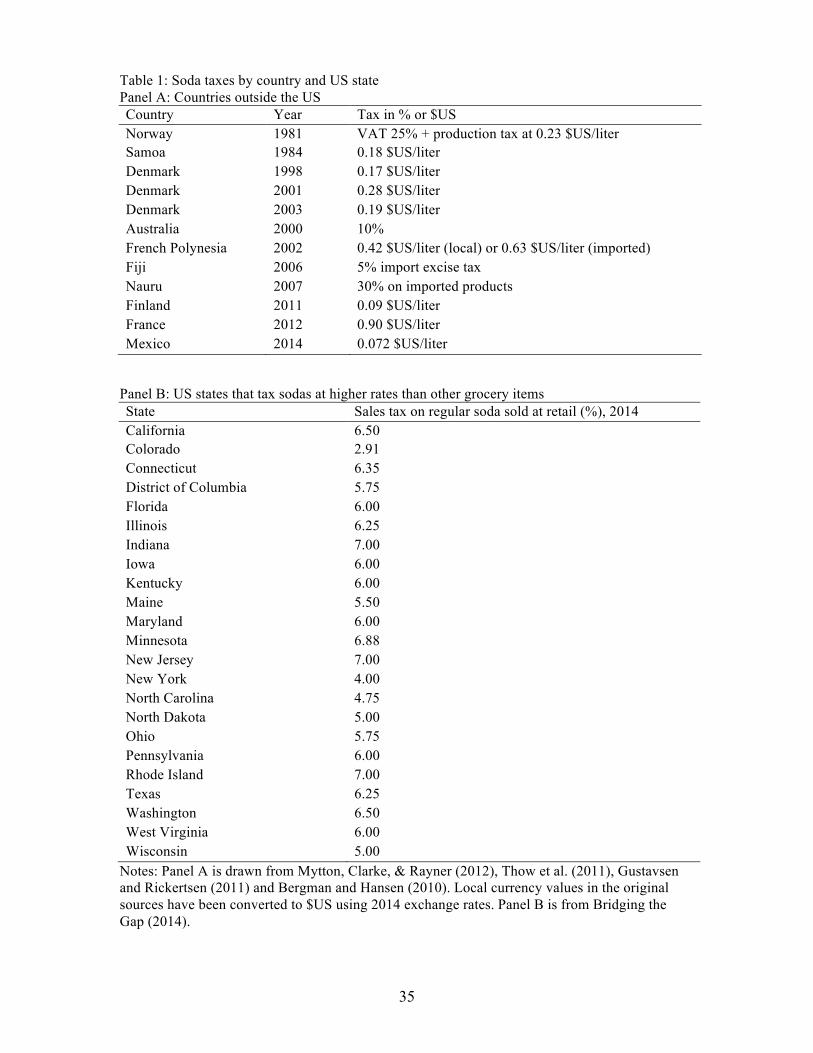
Table 1 compares Mexico’s soda tax with similar taxes elsewhere in the world. Panel A
describes key features of soda taxes imposed by countries outside the U.S. Panel B lists
sales tax rates in U.S. states for regular sodas sold in retail outlets such as grocery stores.
Panel B is limited to states that tax sodas at a higher rate than other grocery products.
With the exception of Illinois, these states impose no sales tax on food, so the tax on
sodas represents the difference between sales taxes imposed on sodas and food. In
international comparison, Mexico’s tax is on the low side, similar to soda taxes in
Australia and Finland. At the same time, however, Mexico’s tax is higher in relative
terms than that imposed by any US state.
B. Previous research on soda taxes and soda prices
Only a handful of studies have analyzed how soda taxes affect soda prices. The earliest
may be Besley & Rosen (1998), who studied longitudinal data across cities to estimate
how sales taxes affected the price of Coca Cola, among other products. They found
evidence of overshifting, that is, evidence that the price rose by more than amount of the
tax. Bergman & Hansen (2010) analyzed price data collected by Statistics Denmark to
compute the Danish CPI. They studied soda tax increases that took effect in 1998 and
7
2001 and a tax cut that took effect in 2003. They found overshifting in response to the
tax increases, but undershifting in response to the tax cut. Berardi, Sevestre, Tepaut, &
Vigneron (2013) estimate the effects of the French soda tax imposed in January 2012
using data provided by an online firm that intermediates drive-through purchases by
consumers from existing brick-and-mortar retail outlets. They report that, six months
after the tax took effect, it had been fully passed through to soda prices. Taxes on other
sugar-sweetened beverages were only partly passed through to consumers. Cawley and
Frisvold (2015) report that Berkeley’s soda tax had little effect on soda prices. Since
consumers can avoid that tax simply by purchasing sodas outside the city limits, retailers
may have limited ability to pass the tax through to consumers.
A related literature analyzes the relationship between soda prices or taxes, soda
consumption, and in some cases, the consumption of potential substitute goods. Block,
Chandra, McManus, & Willett (2010) experimentally manipulated soda prices in a large
hospital and found that consumption fell 26 percent in response to a 35 percent price
increase. Andreyeva, Long, & Brownell (2010) metaanalyzed 14 studies, published
between 1938 and 2007, that estimated the own-price elasticity of demand for soft drinks
in the US. They reported a mean elasticity of -0.79. Another metaanalysis, covering
studies published between 2007 and 2012, estimated the own-price elasticity for sugar-
sweetened sodas in the US to be -1.25 (Powell, Chriqui, Khan, Wada, & Chaloupka,
2013). Fletcher, Frisvold, & Tefft (2010) focused on youths and related consumption of
soft drinks and other beverages to state-level taxes on sodas. They reported that higher
taxes led to moderate reductions in soda consumption, but also to substitution toward
whole milk. Ritter (2015) analyzed the effects of sharp reductions in soda prices that
8
resulted from the entry of a low-cost producer into the Peruvian market for sodas. She
estimated the own-price elasticity of demand for sodas to be -1.3. She found no evidence
that consumers substituted for juice, milk, or bottled water. Finally, Instituto Nacional de
Salud Publica (2014) summarizes results from an unpublished study of the Mexican soda
tax based on data from January to March 2014, that is, the first three months after the tax
took effect. According to the summary, that study analyzed the effect of the tax on
consumption based on data from a consumer panel and found that consumption of sodas
fell by about 10 percent during the first quarter of 2014 relative to the first quarter of
2013. It also reported that consumption of untaxed beverages rose by about 7 percent
during that same period, with consumption of plain water rising by 13 percent.
III. Data
A. Monthly product prices by city
The data I analyze are collected by Mexico’s Consumer Price Index program. These
price data are collected from retail outlets on an ongoing basis, following procedures
spelled out by the ILO’s Consumer Price Index Manual. Prices are obtained for 235,000
specific items each month from products in 283 product categories. Price data are
collected in 46 different cities across the country (Instituto Nacional de Estadistica y
Geographica, 2013).
Each month, Mexico’s National Institute for Statistics and Geography publishes the
average price of each product in each city.1 The products are specified in detail,
including the brand, flavor (if relevant), container, and size of the package. Prices are 1 The data are available at http://www.inegi.org.mx/sistemas/preciospromedio_inpc/ for the period January 2011 to the present.
9
generally quoted per standard unit, that is, per liter or per kilogram. Thus, for example,
one record indicates that, in January 2015 in the greater Mexico City area, the average
liter price of Coca Cola purchased in a six-pack of 12-ounce (355 ml) cans was 22.77
pesos. No information is provided about the number of observations underlying the
published averages, nor about the variance of the underlying item prices.
B. Product categories
I use price data from the INPC product categories sodas, bottled water, juice, and milk.2
Some of these categories consist of a mix of taxed and untaxed products. For example,
the sodas category includes both regular and diet sodas, as well as a few bottled water
products. The bottled water category contains mostly plain water, but also a few flavored
water products that are sweetened with sugar. Likewise, the juice category includes both
100 percent juice products, which are untaxed, plus juice drinks, which are taxed because
they contain added sugar.
In order to distinguish between taxed goods and untaxed substitutes, I created six product
categories from the original four. These are regular sodas, other drinks with added sugar,
diet sodas, bottled water, milk, and pure juice. Regular sodas consist of sugar-sweetened
carbonated beverages. Other drinks with added sugar consist of juice drinks and flavored
water products that are sweetened with sugar. Diet sodas consist of artificially sweetened
carbonated beverages. Bottled water consists of plain water products plus flavored water
products that are not sweetened with sugar. Milk contains all milk products and pure
juice contains all juices that do not contain added sugar.
2 These correspond to the categories refrescos envasados, agua embotellada, jugos o néctares envasados, and leche pasteurizada y fresca.
10
To determine the sugar content of the various products, I relied partly on naming
conventions and also conducted a combination of automated and manual searches of
several Mexican online shopping sites that provide product ingredient lists.3 These
searches identified the sugar content of various products with varying degrees of certainty.
Some naming conventions revealed the sugar content of the product with certainty, such
as the word “diet” in a product name. Likewise, the great majority of products could be
identified with certainty online. However, I inferred some products’ sugar content from
that of a closely related product with the same brand name. For a few products, I was
unable to find any information. I exclude this last group of products from the analysis.
C. Descriptive statistics
I used the price data to construct price indexes for each of the six product categories for
the period January 2011 to June 2015. I then used the monthly Mexican CPI for all
products to convert nominal to real values, setting the base period to December 2013.
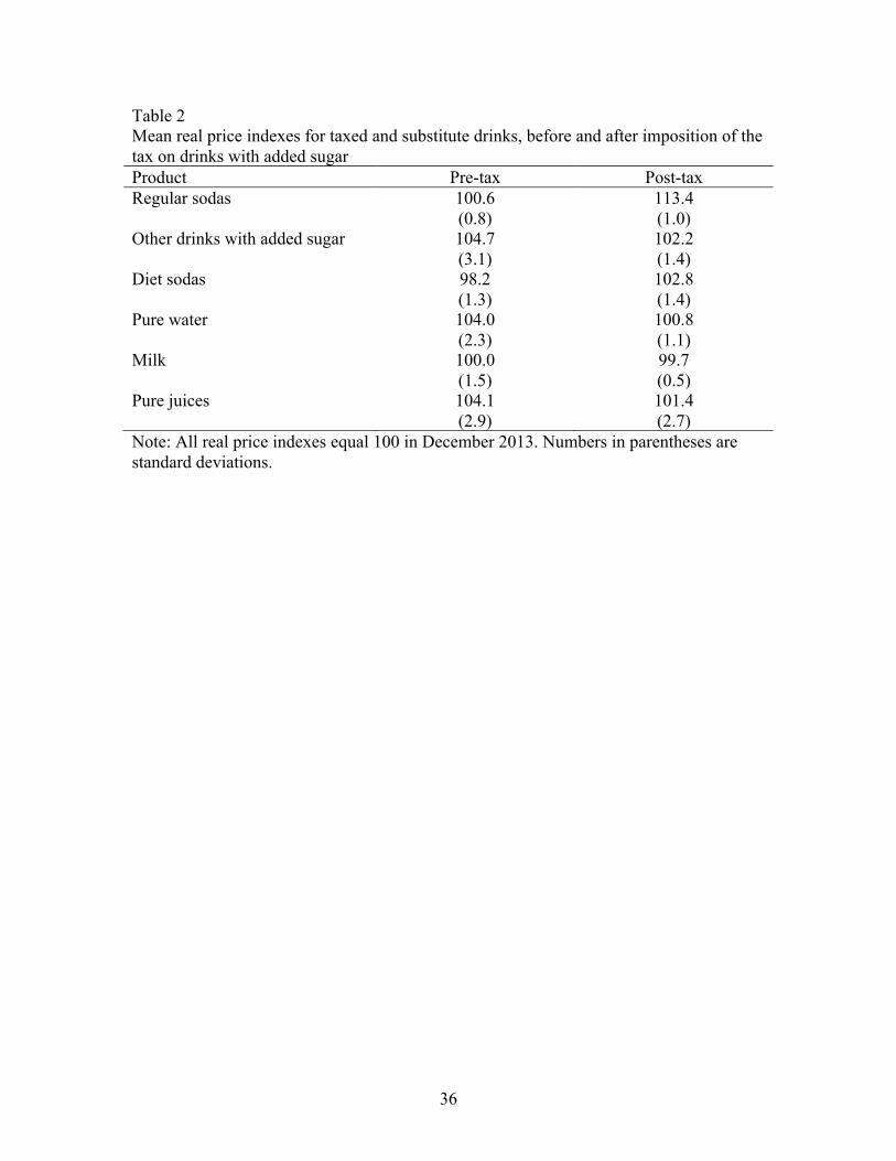
Table 1 reports means of these real price indexes for the periods before and after the soda
tax took effect.
Before the tax was imposed, the mean real price index for regular sodas was 100.6 with
relatively little variation. It jumped by about 13 percent after the tax was imposed. Real
prices of other drinks changed little after the tax. This may indicate that there was little
substitution between regular sodas and untaxed drinks such as diet sodas, pure water,
milk, and pure juices. However, one would have expected the prices of other drinks with
added sugar (DWAS) to rise, since those drinks were also subject to the tax. Further
3 These sites include www.walmart.com.mx, www.superama.com.mx, and www.tudespensa.com/supermercado.
11
inspection showed that the nominal prices of those other DWAS indeed rose after the tax
took effect. However, the nominal prices of those drinks had been roughly constant
during the pre-tax period, meaning that they were falling in real terms. Thus despite the
price increase at the time the tax was imposed, mean real prices in the pre-tax period
were higher on average than mean real prices post-tax. This suggests that it is important
to take pre-tax price trajectories into account in estimating the effect of the tax.
IV. Estimation and inference
I employ two estimation methods that deal differently with pre-tax prices. I discuss the
synthetic control method and the intervention analysis in turn.
A. Synthetic control method
As discussed in the introduction, the soda tax was imposed nationwide all at the same
time. This means there is no comparison group of untaxed markets, for example, that
could be compared to taxed markets in order to identify the effect of the tax. However,
there are many untaxed products that are neither substitutes nor complements for drinks
with added sugar. Thus I estimate the effects of the tax by comparing the prices of taxed
goods and potential substitutes, which I refer to collectively as treatment products, to the
prices of untaxed comparison products.
In principle, one could assign each treatment product to a single comparison product.
This would raise questions as to how the comparison product should be chosen. Instead,
I adapt the approach of ADH and construct a synthetic control product as a convex
combination of comparison products. The comparison goods consist of all untaxed non-
durables whose prices are available from the Mexican Consumer Price Index system and
12
which are not potential substitutes for taxed drinks. This includes roughly 120 products,
mostly food, beverage, and clothing items.4 The synthetic control is that convex
combination of comparison goods whose pre-tax price most closely tracks that of the
treatment product.
To be more precise, let the number of time periods be T = T! + T!, where there are T!
periods before the tax is imposed and T! periods afterwards. Denote the number of
comparison products by J. Let Y! =Y!"Y!"
denote the T x 1 vector of prices for one of
the treatment goods, where Y!" is the T!x 1 vector of pre-tax prices and Y!" is the T!x 1
vector of post-tax prices. Likewise, let Y! =Y!"Y!"
be the T x J matrix of prices of the
comparison goods, where Y!" is the T!x J matrix of pre-tax prices and Y!" is the T!x J
matrix of post-tax prices. Let W be a Jx1 vector of weights. The synthetic comparison
product is chosen by selecting the elements of W to solve
min (Y!"−Y!"W)′V(Y!"−Y!"W) (1)
subject to the constraints that the elements of W all be non-negative and sum to one. The
matrix V is diagonal and non-negative and may place more weight on some observations
than others. The estimated treatment effect, that is, the effect of the tax, is given by
Δ = !!!
(!!!!!!! Y!"# − Y!"#∗ ) , where Y!"# is a typical element of Y!", Y!"#∗ is a typical
element of Y!"∗ = Y!"W∗, and W∗ is the solution to (1).
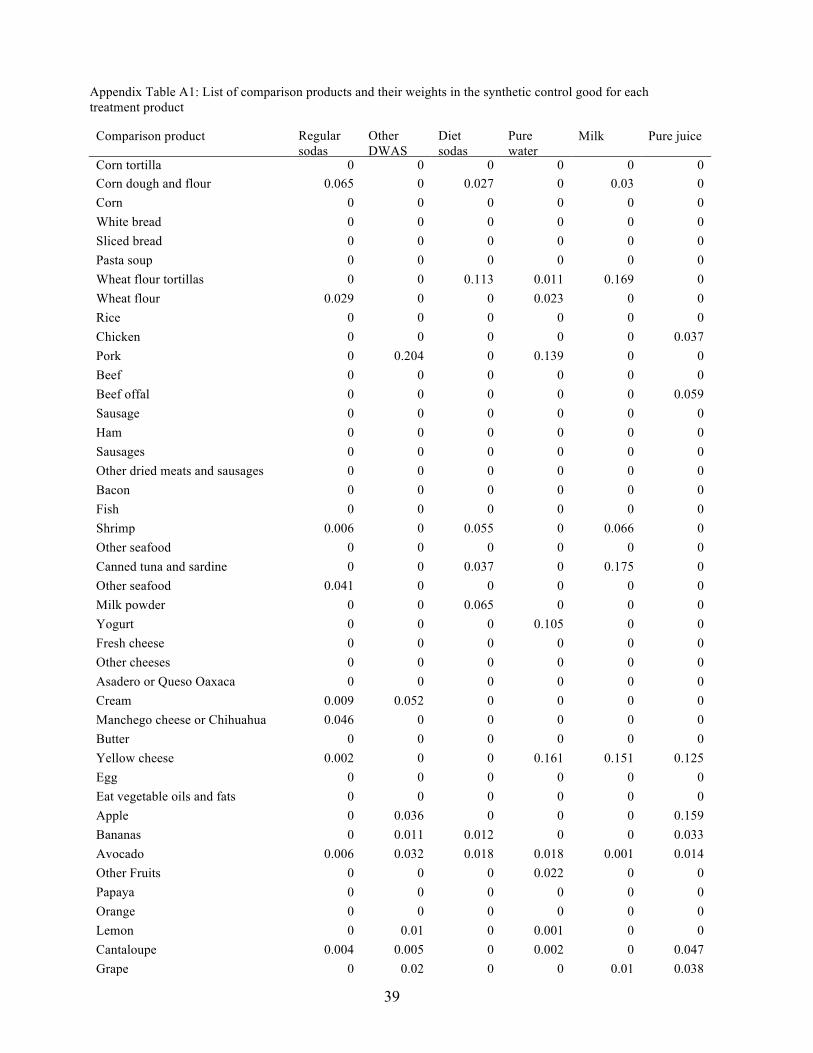
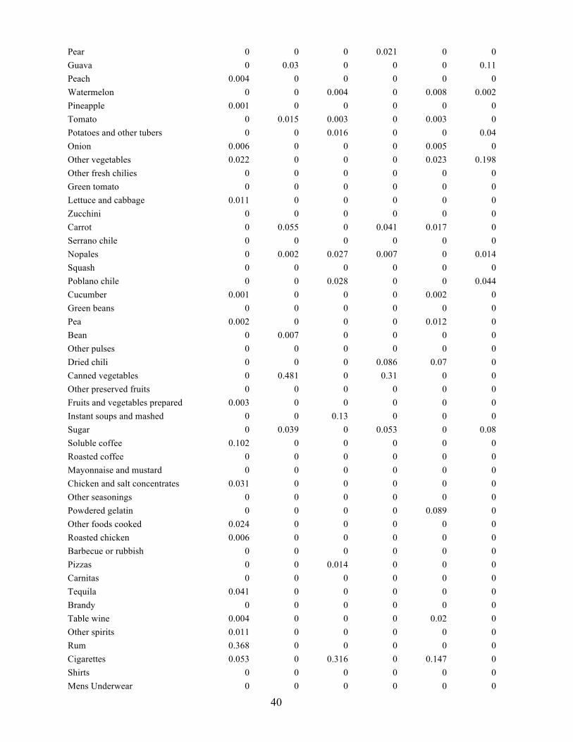
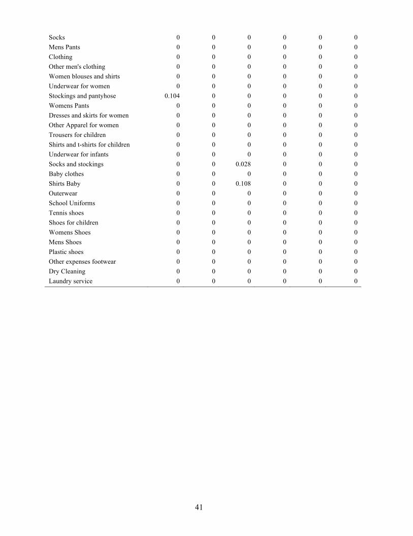
4 A list of these goods appears in Appendix Table 1. In principle one would want to exclude complements as well as substitutes. None of the goods in Appendix Table 1 is an obvious complement to taxed drinks.
13
This can be viewed as a special case of ADH’s original model. They envision a set-up
where there are treatment and comparison units of observation, such as states, and where
the quadratic form in (1) would involve not only pre-treatment values of comparison-unit
outcomes Y!", but also other variables that predict the outcome in the treatment unit.
Lacking such variables, I restrict attention to pre-tax prices of the comparison goods. I
also impose V=I, which treats all pre-tax time periods similarly.5 Thus the synthetic
comparison good is chosen so as to minimize the sum of squared differences over the
pre-tax period between the treatment-good price and the price of the synthetic control
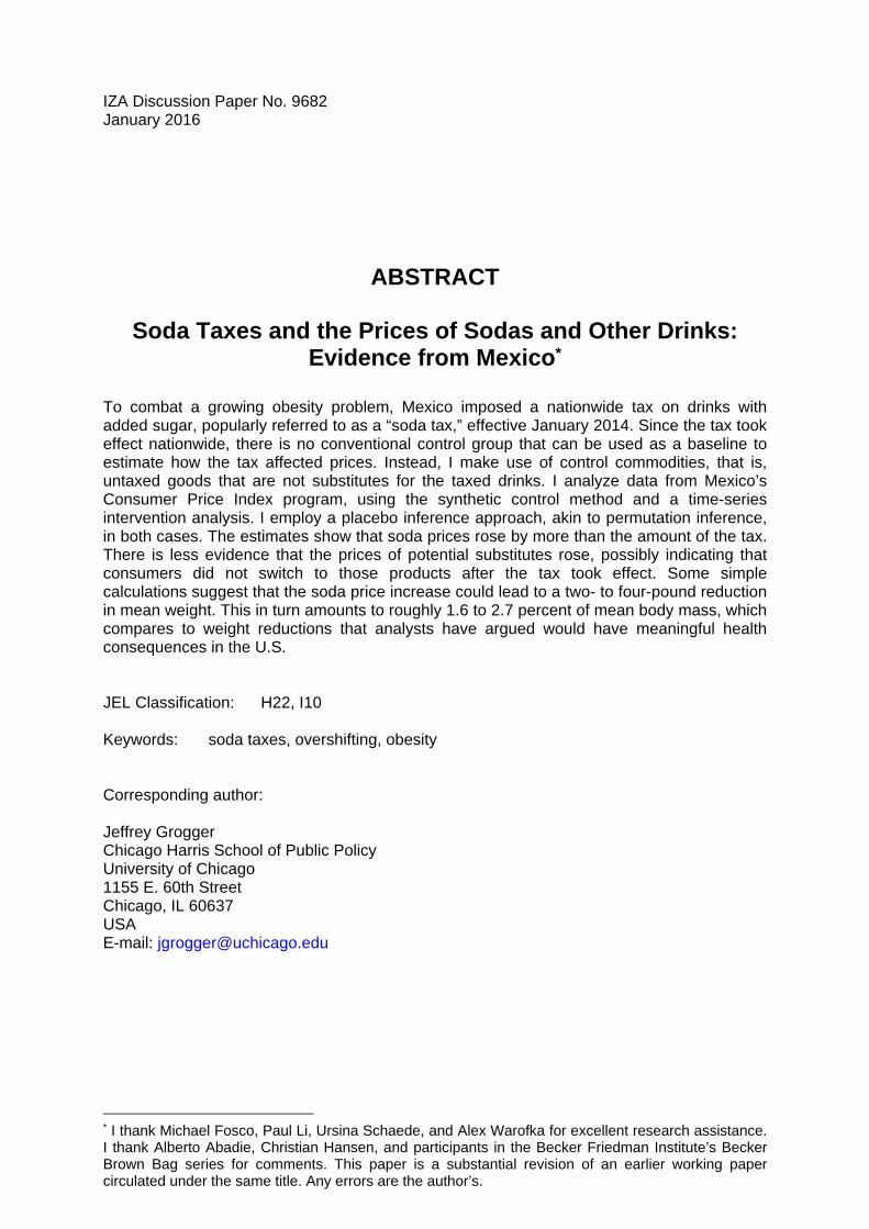
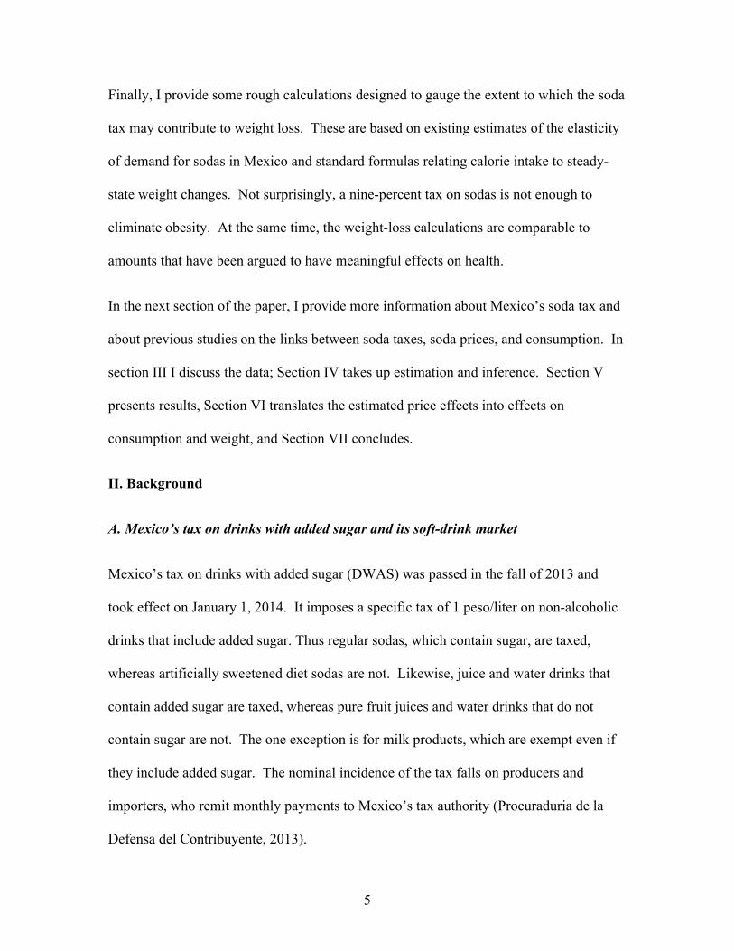
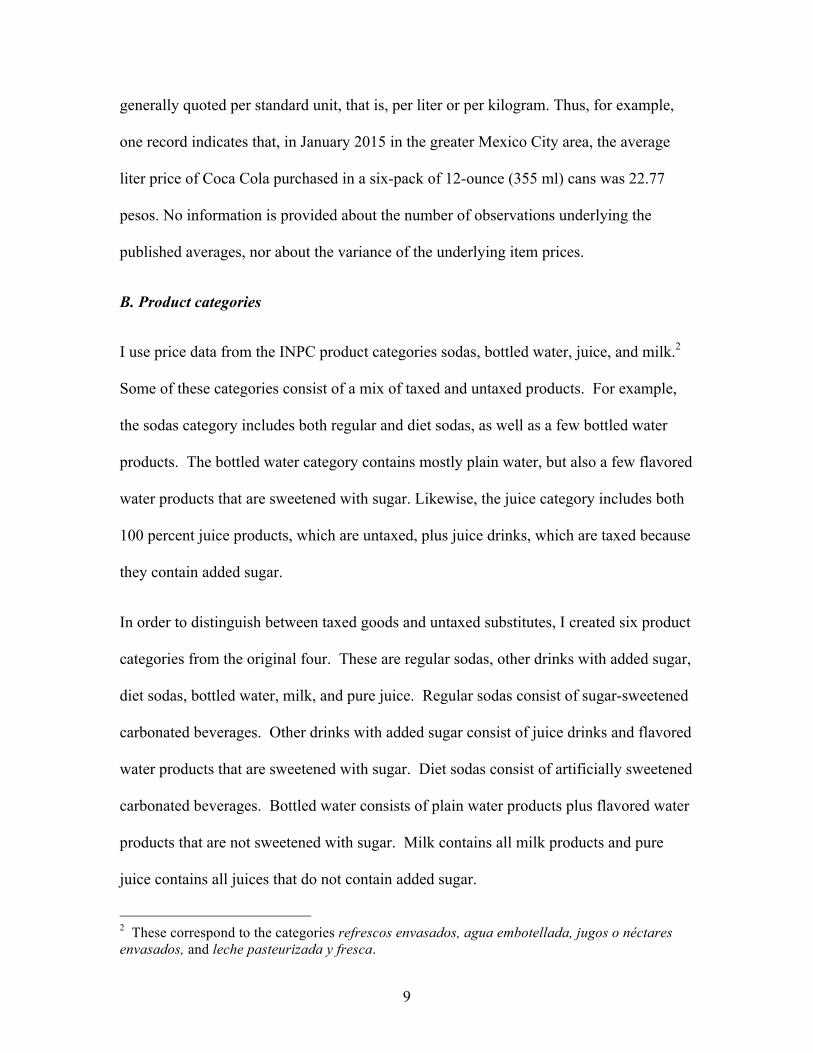
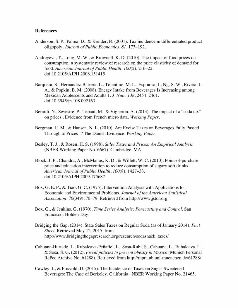
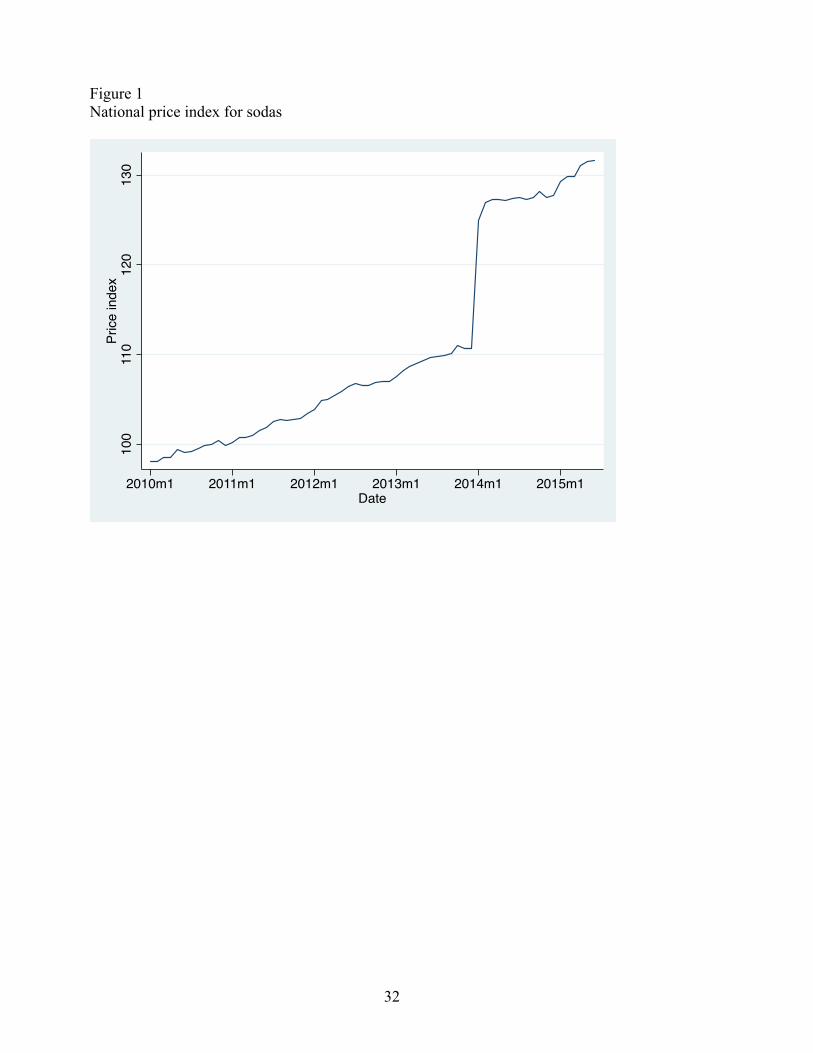
good. Figure 2 plots the price trajectory of the synthetic control good along with the real
price index for regular sodas.6 Prices of the synthetic comparison good track soda prices
closely prior to the imposition of the tax.
ADH propose using placebo methods, akin to permutation inference, to assess
significance. Their argument is that, with aggregate data, relatively little of the
uncertainty about the estimated treatment effect stems from sampling error. In contrast,
there is considerable model uncertainty, that is, uncertainty about the adequacy of the
estimated model to reproduce the counterfactual post-treatment outcomes that would
have been observed in the absence of treatment.
The intuition underlying placebo inference is straightforward. The large jump in soda
prices in Figure 1 might lead one to believe that the tax increased soda prices. However,
that belief would be undermined if the prices of randomly chosen untaxed goods rose
similarly at the same time. Conversely, one’s belief that the tax increased soda prices
5 The estimates reported below were not sensitive to this restriction. 6 The weights used to construct the synthetic comparison product from the untaxed comparison products appear in Appendix Table 2.
14
would be reinforced if the observed change in post-tax soda prices were a sufficiently
extreme event compared to contemporaneous changes in the prices of untaxed goods.
To formalize this idea, ADH propose estimating placebo treatment effects for every unit
in the comparison sample. For each comparison product, I estimate the placebo treatment
effect by treating the product as if it became subject to tax in January 2014, and shifting
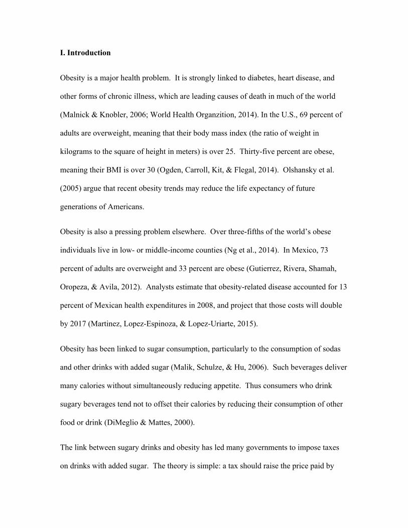
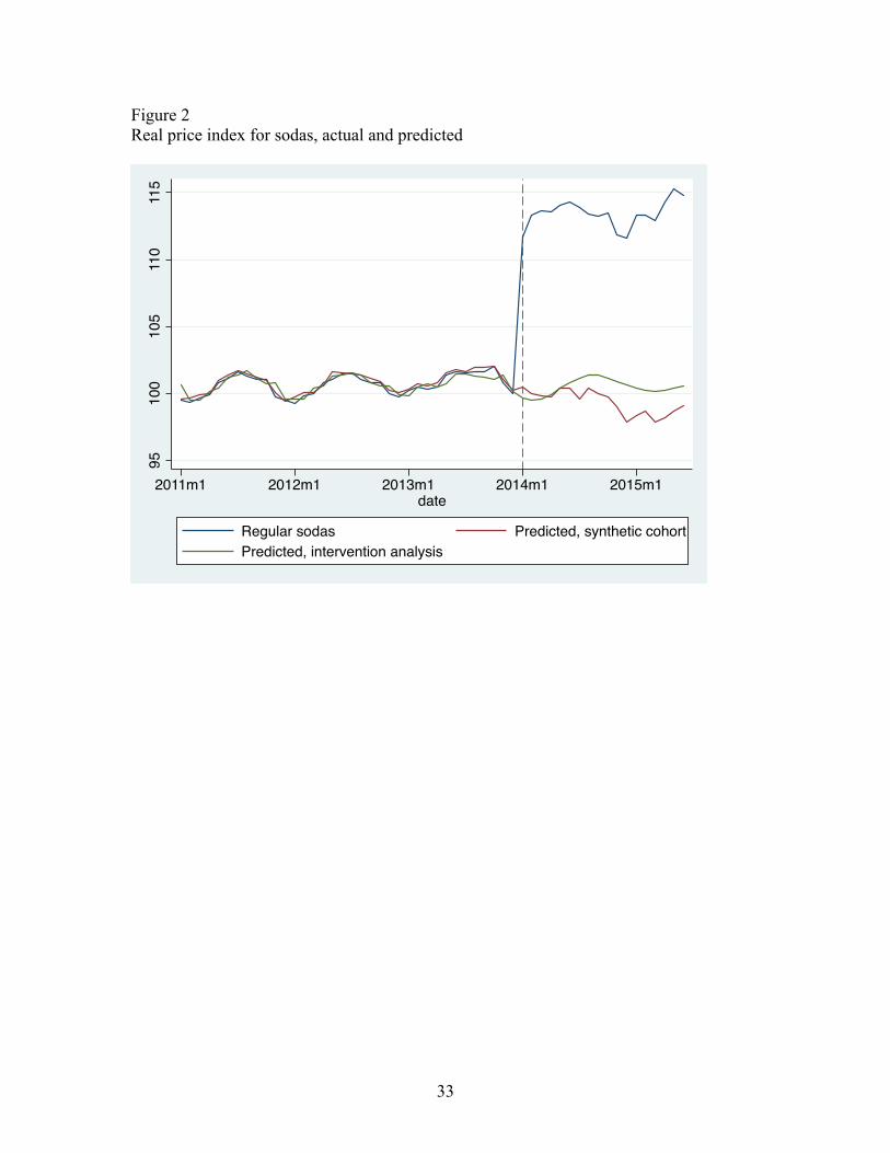
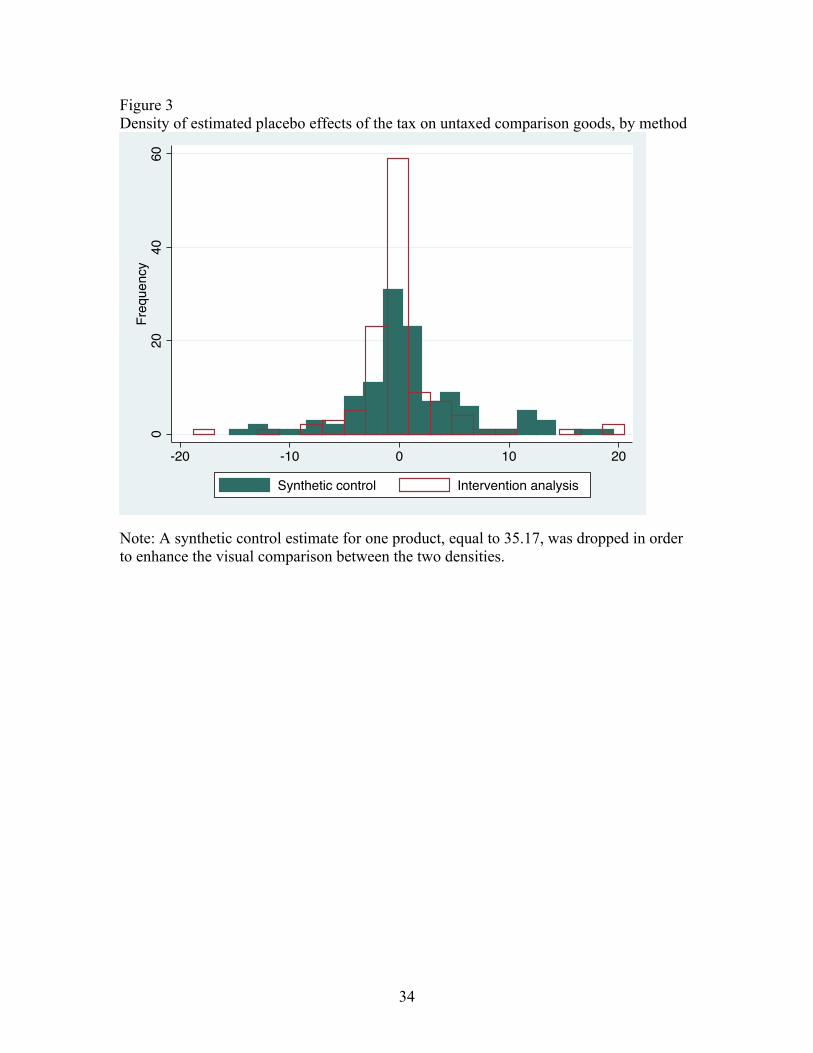
the treatment product to the comparison group. The density of the placebo treatment
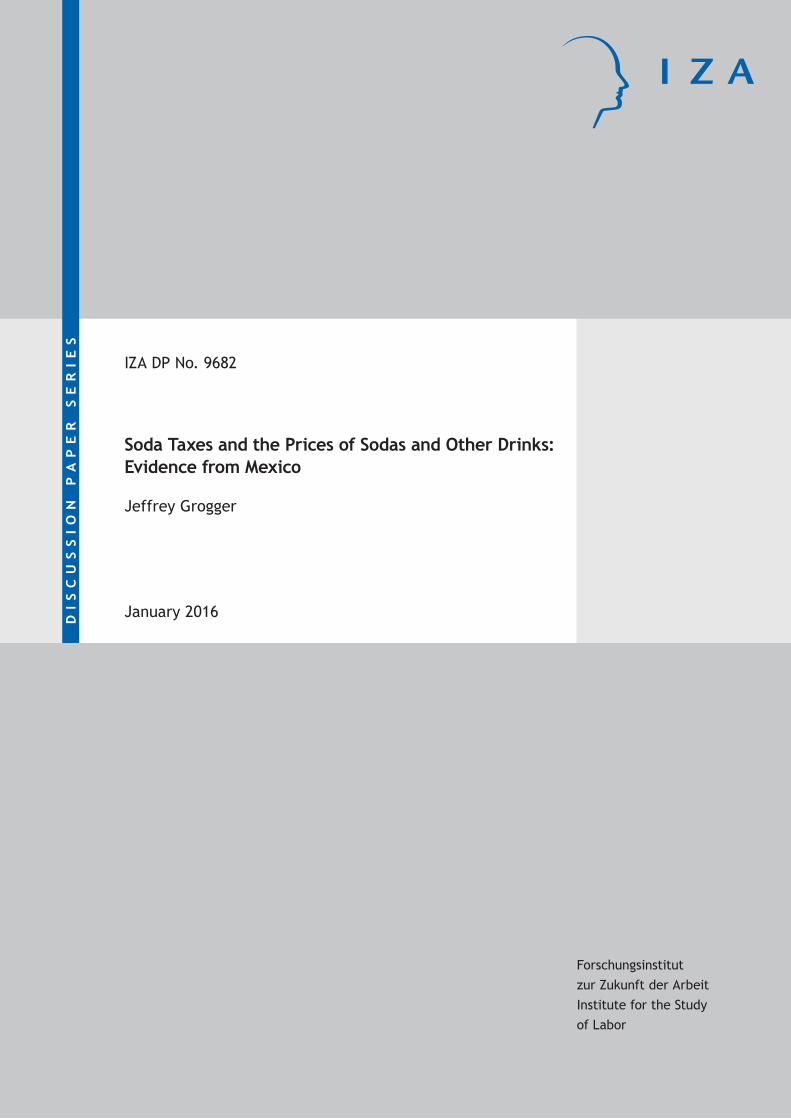
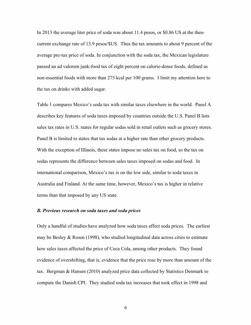
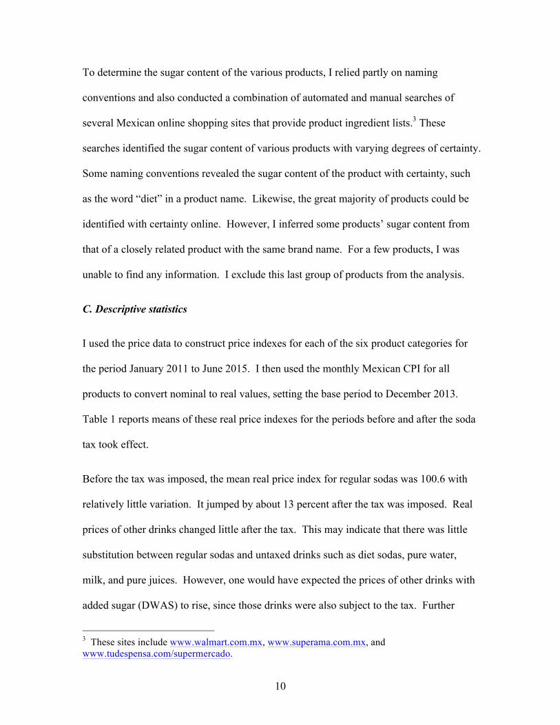
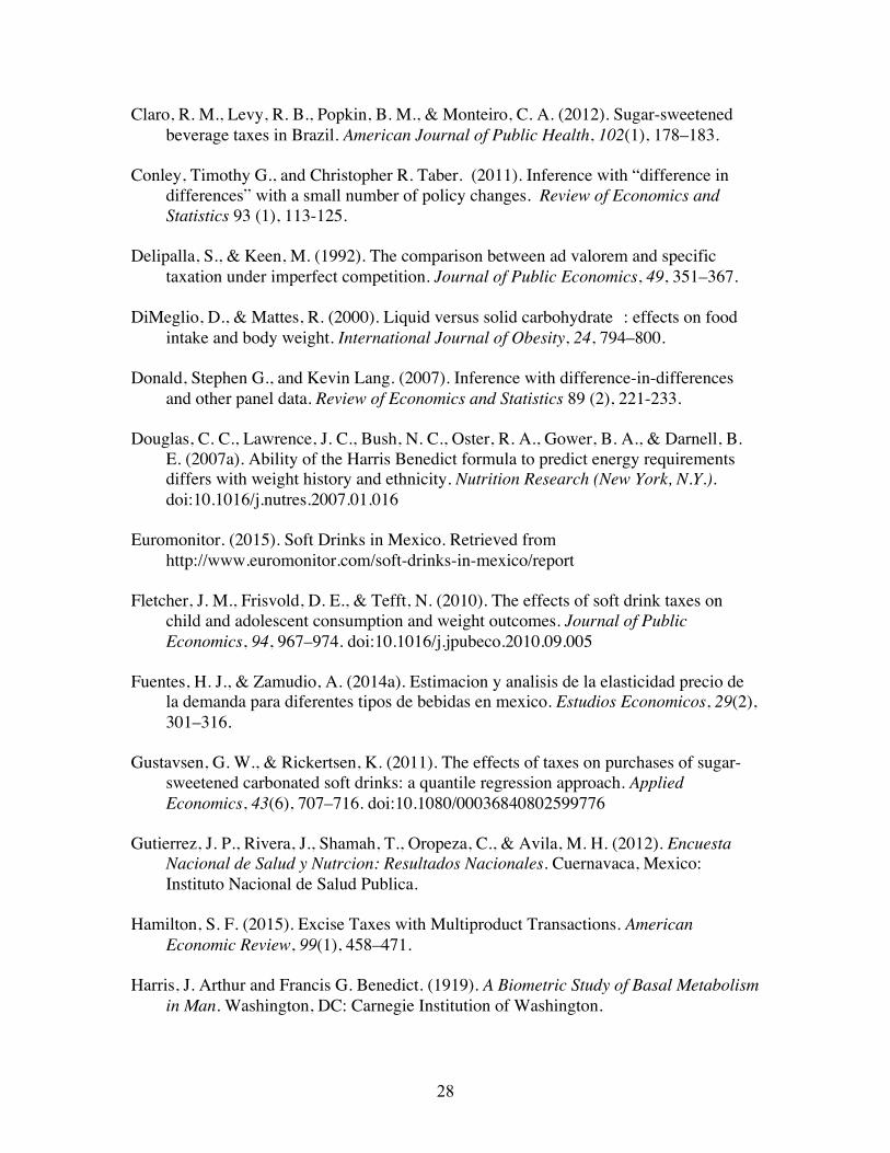
effects is displayed with dark bars in Figure 3.
ADH had a small number of comparisons, and so reported the percentile of their
estimated treatment effect within the distribution of placebo treatment effects. With a
large number of comparison products, I compute confidence intervals, which facilitate
the comparison of precision across estimators. To do so, denote the empirical CDF of
placebo treatment effects by F and let Fp denote its pth percentile. For some
hypothesized value of the treatment effect Δ!, confidence intervals can be derived from
the expression
𝑃 F! ! ≤ Δ− Δ! ≤ F!!! ! = 1− 𝛼
where 𝛼 is the desired confidence level.7
B. Intervention analysis
The idea underlying intervention analysis is to specify a time series model that
adequately describes the evolution of pre-treatment outcomes, then to use that model in
7 With more than 100 comparison products that no ties among the estimated placebo treatment effects, 𝐹! ! and 𝐹!!! ! can be computed uniquely for 𝛼 =.10, which I report below.
15
estimating the effect of treatment via a transfer function. Letting Y!" denote the price of
the treatment good at date t, I estimate an ARIMA model of the form
(1− ϕ L )(1− L)!Y!" = (1− 𝜃 𝐿 )𝜀! t=1,…,TB,
where L is the lag operator such that L!Y! = Y!!!. The autoregressive term ϕ L is a
pth-order polynomial in the lag operator, that is, ϕ L = 1− 𝜌!𝐿 −⋯− 𝜌!𝐿!. The
moving-average term 𝜃 𝐿 is a qth-order polynomial in the lag operator, that is,
θ L = 1− 𝜃!𝐿 −⋯− 𝜃!𝐿!. The disturbance term 𝜀! is assumed to be i.i.d. I select p, d,
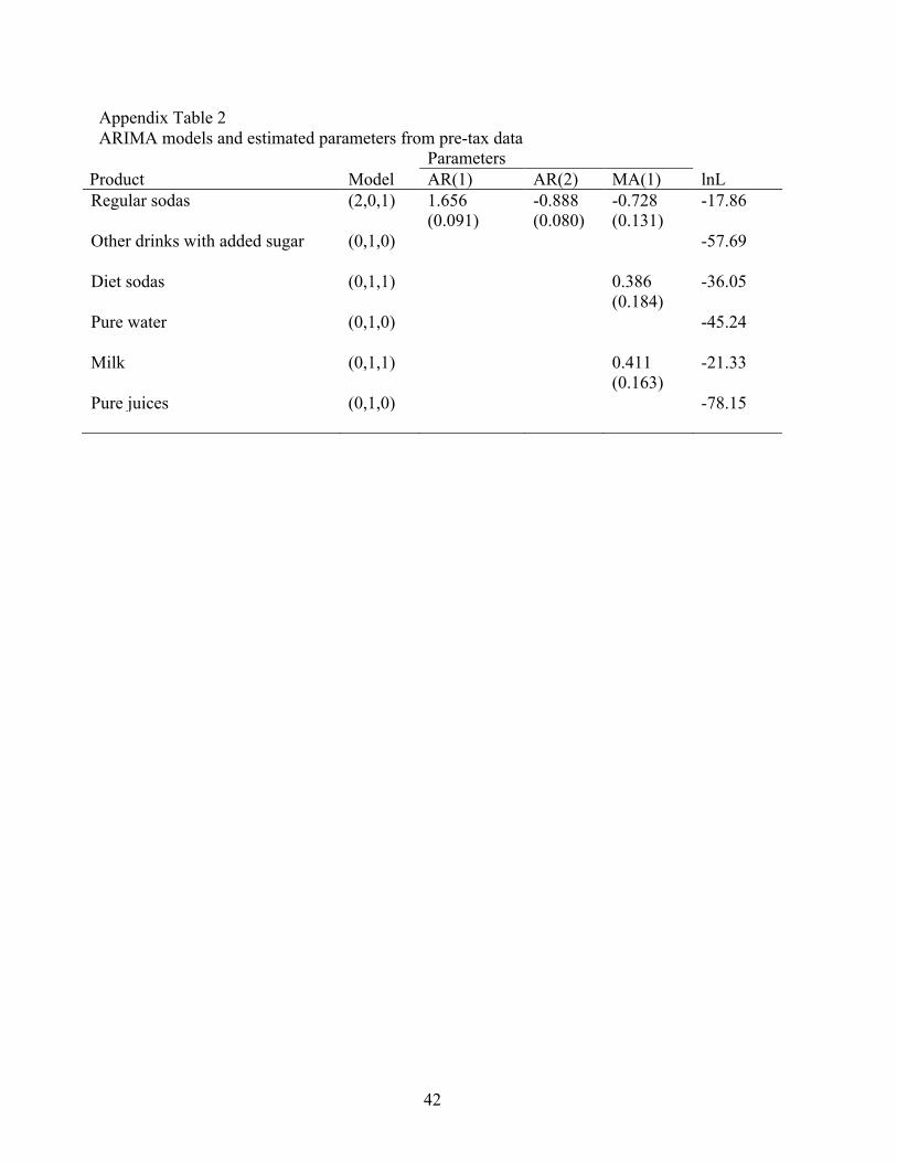
and q so as to minimize Bayes’ Information Criterion (BIC).8
Predicted values from the model estimated from pre-tax soda prices are shown in Figure
2.9 The ARIMA model fits soda prices well over the pre-tax estimation period. Its post-
tax predictions are somewhat higher than those from the synthetic control model, but still
well below actual post-tax prices.
Once the ARIMA parameters p, d, and q have been established based on the pre-tax data,
they are used to estimate the effect of treatment via a transfer function of the form
Y!" = 𝛽! + 𝛽!𝐷! +(!!! ! )
(!!! ! )(!!!)!𝜀! t=1,…,T (2)
where 𝐷! is a dummy variable equal to zero before the intervention and equal to one
beginning January 2014. The term 𝛽! is a constant, which may equal zero, and 𝛽! gives
the effect of treatment, assuming that the effect takes the form of a level shift in Y!". The
8 Models were selected by means of the auto.arima() function of R. Results were similar when I followed the approach of Box and Jenkins (1970). 9 The selected values of p, d, and q, and the estimated coefficients themselves, appear in Appendix Table 2.
16
level-shift assumption seems warranted here by the behavior of soda prices in Figures 1
and 2.
The parameters of equation (2) are estimated by maximum likelihood, assuming 𝜀! to be
normally distributed. This allows for conventional asymptotic inference based on the
estimated covariance matrix of the coefficients. Since I have only 36 pre-tax
observations and 18 post-tax observations, one might question whether asymptotic
inference procedures are appropriate. Furthermore, the conventional approach to
inference does not account for model uncertainty. Although minimizing the BIC
provides an objective approach to model building, there may nevertheless be other
models that provide a reasonable fit to the data, yet yield different estimates of the effects
of the tax. Under such circumstances, it seems desirable to account for model uncertainty
in assessing the precision of the estimated treatment effects.
To do so I apply placebo inference to the intervention analysis. The intuition here is
exactly the same as above: the more extreme is the estimated treatment effect in
comparison to the placebo treatment effects, the greater confidence one has that the tax
raised the price of the taxed good. To estimate the distribution of placebo treatment
effects, I proceed for the comparison goods as for the treatment goods: I first find the
ARIMA model that minimizes the BIC over the pre-tax period, then use that model to
estimate the placebo treatment effect of the tax via the transfer function (2). The density
of the estimated placebo treatment effects is displayed with hollow bars in Figure 3.
Denoting the corresponding CDF by G with pth percentile G!, I construct confidence
intervals for a hypothesized value of the treatment effect 𝛽!" from the expression
17
𝑃 G! ! ≤ 𝛽! − 𝛽!" ≤ G!!! ! = 1− 𝛼.
IV. Results
A. Main results
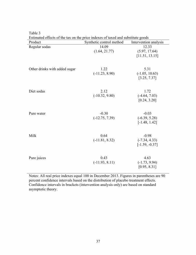
Table 3 presents estimates of the effect of the tax on the real prices of the treatment goods.
The estimates in the first column are Δ from the synthetic cohort approach. The estimates
in the second column are maximum likelihood estimates of β1 from equation (2).
Because the price indexes all equal 100 in December 2013, the estimates can be
interpreted as the proportionate change in price due the tax, relative to the price in the last
month before the tax took effect.
The first row presents estimates for the price of regular sodas. The estimates from the
synthetic control method and the intervention analysis are fairly close. The former
indicates that soda prices rose 14.09 percent in response to the tax, whereas the latter
shows that the tax raised soda prices by 12.33 percent. The placebo confidence intervals
in parentheses correspond to the null hypothesis that the true effect of the tax equals zero
and a 90 percent confidence level. Neither confidence interval includes zero, indicating
that both estimates are significant at the 10 percent level.10
The confidence interval in column (1) is wider than that in column (2), suggesting that
the synthetic control method is subject to greater uncertainty than the intervention
analysis. This idea is confirmed in Figure 3, which plots the frequency distributions of
the placebo treatment effects obtained by each method. The density from the intervention
10 Both estimates were at the 97th percentile of their placebo treatment effect distributions.
18
analysis has much more mass around zero, and less mass in the tails, than the density
from the synthetic control method.11
One potential explanation for this is that the synthetic control method generally involves
more estimated parameters than the intervention analysis. Another explanation may be
more intuitive. Both methods estimate the placebo treatment effect at least heuristically
as the difference between the actual post-tax price and the forecasted post-tax price,
where the forecast is based on pre-tax data. The synthetic control product is chosen to
match the price of the (placebo) treatment product, whereas the pre-tax ARIMA model
used in the intervention analysis is designed to capture the dynamics of the price series.
The ARIMA method may have an advantage in forecasting, which results in placebo
treatment effects consistently closer to zero for products not subject to tax.
For the intervention analysis, 90 percent confidence intervals based on standard
asymptotic theory appear in brackets below the placebo confidence interval. The
standard confidence interval is much narrower than its placebo counterpart. However,
the standard asymptotics do not account for model uncertainty. Judging from the relative
widths of the two confidence intervals, model uncertainty seems to be a large component
of the overall uncertainty surrounding the estimated effect of the tax.
Moving beyond significance levels, both the synthetic control and the intervention
analysis estimates indicate that prices rose by more than the amount of the tax, which was
one peso/liter. Relative to the 2013 average price of 11.4 pesos, the synthetic control
estimate of the price change due to the tax is 1.61 pesos, whereas the intervention 11 To construct Figure 3, I deleted one synthetic-control placebo effect with a value of 35.17 in order to make the differences between the densities more apparent. However, I included it in the calculation of the confidence interval.

19
analysis estimate is 1.41 pesos. Such overshifting of the tax is inconsistent with
competitive models of market behavior, but may arise in models of imperfect competition,
as mentioned above. Considering that Coca-Cola has roughly a 70 percent share of
Mexico’s soda market, and PepsiCo accounts for another 15 percent (Smolinski & Yuk,
2013), overshifting may not seem so surprising.
The next estimates in Table 3 show the effect of the tax on other drinks with added sugar.
Both estimates are positive, but the intervention analysis estimate is about four times
larger than the synthetic control estimate. Neither estimate is significant based on the
placebo confidence intervals.
Both estimates of the effect of the tax on diet sodas are similar. Both are positive,
consistent with consumers’ substituting from regular toward artificially sweetened sodas.
However, neither estimate is significant based on the placebo confidence intervals. There
is no evidence that the tax had much effect on the prices of either pure water or milk, as
shown in the next two lines of the Table.
The final set of estimates pertains to pure fruit juices. Both estimates are positive, but the
estimate based on intervention analysis is 10 times larger than the estimate based on the
synthetic control method. Neither estimate is significant based on the placebo inference
procedure. The intervention analysis estimate is significant based on standard
asymptotics, but that approach fails to account for model uncertainty.
Before proceeding, it is worthwhile to summarize the evidence and make note of some
limitations. Whereas the analysis shows clearly that the tax raised soda prices, it shows
little if any effect on the other taxed drinks. One might have expected a smaller rise there
20
than for sodas, since the market for sweetened drinks other than sodas is less
concentrated than the market for sodas (Euromonitor 2015). Nonetheless, economic
theory generally predicts that taxes should raise prices, irrespective of market structure.
The puzzle only deepens when one looks in more detail at the estimate from the
intervention analysis. Although this estimate is fairly large, it comes from an ARIMA (0,
1, 0) model (see Appendix Table 2), meaning that the estimate is based on the change in
price between two months, December 2013 and January 2014. Recall from above that
the price of other drinks with added sugar jumped as the tax was imposed, but then fell in
real terms thereafter. This suggests that the intervention analysis probably overstates the
effect of the tax on these drinks.
This case highlights a potential weakness of intervention analysis: depending on the
model that provides the best pre-intervention fit, it can actually exacerbate an existing
small-numbers problem. At the same time, this example underscores the importance of
adopting an approach to inference that is not reliant on conventional asymptotic theory.
As for the other drinks in Table 3, there is little evidence that the tax raised prices, which
one would have expected if consumers had switched from the taxed drinks to untaxed
substitutes. Indeed, three of the eight estimates are negative rather than positive. The
largest positive estimate, for pure juices from the intervention analysis, is again based on
an ARIMA (0, 1, 0) model and thus the change in price between December 2013 and
January 2014. On the whole, the estimates suggest either that consumers did not
substitute toward untaxed drinks, or that the supply curve for those products is flat.
21
B. Robustness
I address three issues here that bear on the robustness of the estimates. The first involves
the level of certainty with which I was able to assess the sugar content of some products,
particularly those in the other DWAS, pure water, and pure juice categories. As
mentioned above, I excluded from the estimation sample all products about whose sugar
content I could find no information. I also experimented with dropping products whose
sugar content was gleaned indirectly from similar products. This had no material effect
on the results.
Second, some Mexican consumers may be able to circumvent the tax by crossing the
border and purchasing drinks in the United States. To check against this possibility, I
reestimated the models above after dropping cities near the border from the sample. This
likewise had little effect on the results.
Finally, I reestimated synthetic control models after dropping the clothing items from the
set of comparison products. ADH argue that restricting attention to comparison units that
share characteristics with the treatment units may help reduce bias. Although beverages,
food, and clothing are all non-durable goods, one could take the view that clothing is
different from the other two because it is typically purchased less frequently. I therefore
reestimated the treatment effects and the distributions of the placebo treatment effects
after dropping the clothing items from the comparison goods. This had very little effect
on the treatment effects and none on inference. For symmetry, I also recomputed the
confidence intervals for the treatment effects from the intervention analysis after
22
dropping the placebo treatment effects for the clothing items. This likewise had no effect
on significance levels.
V. From prices to pounds
In this section I provide a rough estimate of how the price changes estimated above may
affect consumption and ultimately weight. To estimate the consumption change, I use
data on pre-tax consumption levels and existing estimates of Mexico’s demand elasticity
for sodas. To estimate steady-state weight changes that stem from the estimated
consumption change, I use the Harris-Benedict formula.
According to the market research firm Euromonitor (2015), Mexicans consumed 139.4
liters of soda per person in 2013. Recent estimates of the demand elasticity for sodas in
Mexico fall in a range between -1 and -1.3 (Valero 2006; Barquera, et al 2008; Cahuana
et al 2012; Castro-Carrillo, et al 2014). I calculate estimated consumption changes based
on both of these elasticities and on both estimates from above of the effect of the tax on
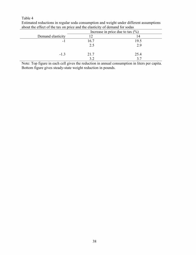
soda prices. The results appear as the top entries in each cell of Table 4. They show that
the soda tax could lead to a decrease in consumption of somewhere between 16.7 and
25.4 liters per person per year.
To calculate the mean weight change resulting from that reduction, I use the Harris-
Benedict formula. That formula first calculates the basal metabolic rate, or BMR, also
known as resting energy expenditure, which is the daily caloric expenditure of the human
body at rest. This expression can be written as
BMR = α+ δW,
23
where W is weight; the constant term α is a function of age, height, and sex; and the
weight coefficient δ is a function of sex. Roza and Shizgal (1984) report that δ=13.4 for
men and δ=9.3 for women.12
To determine actual energy expenditure, BMR is multiplied by an activity factor 𝛾. For
persons with a sedentary lifestyle, 𝛾 =1.2. For persons with a moderately active lifestyle,
𝛾 =1.5 (Douglas et al 2007).
In steady state, energy intake I equals energy expenditure. This yields the steady-state
relationship between daily calorie intake and weight
I = 𝛾 (α + δW),
from which the steady-state change in weight Δ𝑊 owing to a change in calorie intake Δ𝐼
is Δ𝑊 = ΔI/(γδ).
To calculate the weight change resulting from the consumption changes in Table 4, I
assume that each liter of soda contains 400 calories and choose the moderate activity
factor γ =1.5. If the Mexican population is actually more sedentary, on average, weight
loss would be greater than what I calculate; if it is more active, then weight loss would be
less. I also assume that half the Mexican population is male and half female. Finally, I
further assume that calorie reductions due to decreases in soda consumption are not offset
by increases in calories from other sources. This may be justified by the evidence in
Table 3, which showed no significant evidence of substitution between regular sodas and
other caloric drinks. However, if some of those calorie reductions are offset, then weight
loss would be less than my calculations suggest. 12 The corresponding values from the original Harris and Benedict (1919) study were 13.8 and 9.6.
24
The steady-state weight loss calculations appear as the bottom entries in each cell of
Table 4. With a 12-percent increase in soda prices and a demand elasticity of -1, mean
steady-state weight loss is 2.5 pounds. At the other end of the spectrum, with a 14
percent price increase and a demand elasticity of -1.3, steady-state weight loss is 3.7
pounds.
Is weight loss of this magnitude meaningful? It is clearly insufficient to eliminate obesity
or overweight. However, Wang et al (2007) and Levi et al. (2012), using U.S. data,
suggest that a reduction in mean BMI on the order of 1 to 5 percent may be sufficient to
generate meaningful improvements in health. Mexico is not the US, but the similarity of
weight distributions in the two countries might lead one to expect that a similar reduction
in mean BMI in Mexico could have important effects on health there.
Calculations based on data from Mexico’s National Health and Nutrition Survey show
that mean adult BMI would fall by 1 percent if every Mexican adult were to lose about
1.6 pounds. Thus the weight loss calculations in Table 4 range from 1.6 to 2.7 percent of
mean BMI. Subject to the caveats discussed above, weight loss due to the soda tax could
result in weight loss within the range of 1 to 5 percent of mean BMI.
V. Summary and conclusions
Obesity and its consequences represent a pressing public health problem. To staunch the
rise in obesity, Mexico imposed a tax, effective January 2014, on drinks that contain
added sugar, commonly referred to as a soda tax. Several other countries have imposed
similar taxes, and they are currently under discussion in countries as diverse as Colombia
and the United Kingdom.
25
Analyzing the effect of the tax on prices is complicated by the fact that Mexico’s tax was
imposed nationwide all at once. This means there is no conventional control group that
one could use as a baseline for estimating the effect of the tax. Instead, I make use of
control commodities, that is, untaxed comparison goods that are not substitutes for the
taxed products.
I take two approaches to estimation, one based on the synthetic control method and the
other based on intervention analysis. In both cases I employ placebo methods for
inference. Comparing the placebo approach to conventional inference methods (in the
case of the intervention analysis) suggests that much of the imprecision in the estimates
stems not from conventional sampling error, but from model uncertainty. The
intervention analysis also seems to yield somewhat more precise estimates than the
synthetic control method.
Both sets of estimates show that soda prices rose by more than the amount of the tax.
Such overshifting has also been found in other studies of soda taxes and is consistent with
the considerable level of concentration found in Mexico’s soda market. At the same time,
the price of other taxed drinks rose little if at all. There is little evidence that the price of
untaxed drinks rose, which could have happened if consumers had substituted away from
sodas and toward those drinks.
Under some assumptions, one can predict how population weight should respond to the
price increase for sodas. Those calculations show that mean weight among adults could
fall by roughly two to four pounds. At first glance this seems small. However, recent
research suggests that reducing mean BMI by 1 to 5 percent could have meaningful

26
effects on health. The predicted weight reductions stemming from the soda tax are within
that range.
.
References
Anderson, S. P., Palma, D., & Kreider, B. (2001). Tax incidence in differentiated product oligopoly. Journal of Public Economics, 81, 173–192.
Andreyeva, T., Long, M. W., & Brownell, K. D. (2010). The impact of food prices on consumption: a systematic review of research on the price elasticity of demand for food. American Journal of Public Health, 100(2), 216–22. doi:10.2105/AJPH.2008.151415
Barquera, S., Hernandez-Barrera, L., Tolentino, M. L., Espinosa, J., Ng, S. W., Rivera, J. A., & Popkin, B. M. (2008). Energy Intake from Beverages Is Increasing among Mexican Adolescents and Adults 1. J. Nutr, 138, 2454–2461. doi:10.3945/jn.108.092163
Berardi, N., Sevestre, P., Tepaut, M., & Vigneron, A. (2013). The impact of a “soda tax” on prices . Evidence from French micro data. Working Paper.
Bergman, U. M., & Hansen, N. L. (2010). Are Excise Taxes on Beverages Fully Passed Through to Prices ? The Danish Evidence. Working Paper.
Besley, T. J., & Rosen, H. S. (1998). Sales Taxes and Prices: An Empirical Analysis (NBER Working Paper No. 6667). Cambridge, MA.
Block, J. P., Chandra, A., McManus, K. D., & Willett, W. C. (2010). Point-of-purchase price and education intervention to reduce consumption of sugary soft drinks. American Journal of Public Health, 100(8), 1427–33. doi:10.2105/AJPH.2009.175687
Box, G. E. P., & Tiao, G. C. (1975). Intervention Analysis with Applications to Economic and Environmental Problems. Journal of the American Statistical Association, 70(349), 70–79. Retrieved from http://www.jstor.org
Box, G., & Jenkins, G. (1970). Time Series Analysis: Forecasting and Control. San Francisco: Holden-Day.
Bridging the Gap. (2014). State Sales Taxes on Regular Soda (as of January 2014). Fact Sheet. Retrieved May 12, 2015, from http://www.bridgingthegapresearch.org/research/sodasnack_taxes/
Cahuana-Hurtado, L., Rubalcava-Peñafiel, L., Sosa-Rubi, S., Cahuana, L., Rubalcava, L., & Sosa, S. G. (2012). Fiscal policies to prevent obesity in Mexico (Munich Personal RePec Archive No. 61288). Retrieved from http://mpra.ub.uni-muenchen.de/61288/
Cawley, J., & Frisvold, D. (2015). The Incidence of Taxes on Sugar-Sweetened Beverages: The Case of Berkeley, California. NBER Working Paper No. 21465.
28
Claro, R. M., Levy, R. B., Popkin, B. M., & Monteiro, C. A. (2012). Sugar-sweetened beverage taxes in Brazil. American Journal of Public Health, 102(1), 178–183.
Conley, Timothy G., and Christopher R. Taber. (2011). Inference with “difference in differences” with a small number of policy changes. Review of Economics and Statistics 93 (1), 113-125.
Delipalla, S., & Keen, M. (1992). The comparison between ad valorem and specific taxation under imperfect competition. Journal of Public Economics, 49, 351–367.
DiMeglio, D., & Mattes, R. (2000). Liquid versus solid carbohydrate : effects on food intake and body weight. International Journal of Obesity, 24, 794–800.
Donald, Stephen G., and Kevin Lang. (2007). Inference with difference-in-differences and other panel data. Review of Economics and Statistics 89 (2), 221-233.
Douglas, C. C., Lawrence, J. C., Bush, N. C., Oster, R. A., Gower, B. A., & Darnell, B. E. (2007a). Ability of the Harris Benedict formula to predict energy requirements differs with weight history and ethnicity. Nutrition Research (New York, N.Y.). doi:10.1016/j.nutres.2007.01.016
Euromonitor. (2015). Soft Drinks in Mexico. Retrieved from http://www.euromonitor.com/soft-drinks-in-mexico/report
Fletcher, J. M., Frisvold, D. E., & Tefft, N. (2010). The effects of soft drink taxes on child and adolescent consumption and weight outcomes. Journal of Public Economics, 94, 967–974. doi:10.1016/j.jpubeco.2010.09.005
Fuentes, H. J., & Zamudio, A. (2014a). Estimacion y analisis de la elasticidad precio de la demanda para diferentes tipos de bebidas en mexico. Estudios Economicos, 29(2), 301–316.
Gustavsen, G. W., & Rickertsen, K. (2011). The effects of taxes on purchases of sugar-sweetened carbonated soft drinks: a quantile regression approach. Applied Economics, 43(6), 707–716. doi:10.1080/00036840802599776
Gutierrez, J. P., Rivera, J., Shamah, T., Oropeza, C., & Avila, M. H. (2012). Encuesta Nacional de Salud y Nutrcion: Resultados Nacionales. Cuernavaca, Mexico: Instituto Nacional de Salud Publica.
Hamilton, S. F. (2015). Excise Taxes with Multiproduct Transactions. American Economic Review, 99(1), 458–471.
Harris, J. Arthur and Francis G. Benedict. (1919). A Biometric Study of Basal Metabolism in Man. Washington, DC: Carnegie Institution of Washington.
29
Instituto Nacional de Estadistica y Geographica. (2013). Indice Nacional de Precios al Consumidor: Documento Metodologico. Mexico City, Mexico. Retrieved from https://www.google.com/url?sa=t&rct=j&q=&esrc=s&source=web&cd=1&cad=rja&uact=8&ved=0CB8QFjAA&url=http%3A%2F%2Fwww.inegi.org.mx%2Fest%2Fcontenidos%2FProyectos%2FINP%2FDefault.aspx%3F_file%3Ddocumento_metodologico_inpc_inegi.pdf&ei=5BxSVZ3bKtb8oQSKiIHIAQ&us
Instituto Nacional de Salud Publica. (2014). Resultados preliminares sobre los efectos del impuesto de un peso a bebidas azucuradas en Mexico. Retrieved May 12, 2014, from http://www.insp.mx/epppo/blog/preliminares-bebidas-azucaradas.html
Levi, J., Segal, L. M., St. Laurent, R., Lang, A., & Rayburn, J. (2012). F as in Fat: How Obesity Threatens America’s Health. Washington, DC: Trust for America’s Health.
Malik, V. S., Schulze, M. B., & Hu, F. B. (2006). Intake of sugar-sweetened beverages and weight gain : a systematic review. American Journal of Clinical Nutrition, 84, 274–288.
Malnick, S. D. H., & Knobler, H. (2006). The medical complications of obesity. Quarterly Journal of Medicine, 99(9), 565–579. doi:10.1093/qjmed/hcl085
Martinez, A. G., Lopez-Espinoza, A., & Lopez-Uriarte, P. J. (2015). Mexico obeso: actualidades y perspectivas. Guadalajara, Mexico: University of Guadalajara.
Mytton, O. T., Clarke, D., & Rayner, M. (2012). Taxing unhealthy food and drinks to improve health. BMJ (Clinical Research Ed.), 344, e2931. doi:10.1136/bmj.e2931
Ng, M., Fleming, T., Robinson, M., Thomson, B., Graetz, N., Margono, C., … Gakidou, E. (2014). Global, regional, and national prevalence of overweight and obesity in children and adults during 1980-2013: a systematic analysis for the Global Burden of Disease Study 2013. Lancet, 6736(14), 1–16. doi:10.1016/S0140-6736(14)60460-8
Ogden, C. L., Carroll, M. D., Kit, B. K., & Flegal, K. M. (2014). Prevalence of childhood and adult obesity in the United States, 2011-2012. JAMA : The Journal of the American Medical Association, 311(8), 806–14. doi:10.1001/jama.2014.732
Olshansky, S. Jay, et al. (2005). “A Potential Decline in Life Expectancy in the United States in the 21st Century.” New England Journal of Medicine 352 (11) 1138-1145.
Poterba, J. M. (1996). Retail price reactions to changes in state and local sales taxes, National Tax Journal 49(2), 165–176.
Powell, L. M., Chriqui, J., & Chaloupka, F. J. (2009). Associations between State-level Soda Taxes and Adolescent Body Mass Index. Journal of Adolescent Health, 45. doi:10.1016/j.jadohealth.2009.03.003
30
Powell, L. M., Chriqui, J. F., Khan, T., Wada, R., & Chaloupka, F. J. (2013). Assessing the potential effectiveness of food and beverage taxes and subsidies for improving public health: a systematic review of prices, demand and body weight outcomes. Obesity Reviews : An Official Journal of the International Association for the Study of Obesity, 14(2), 110–28. doi:10.1111/obr.12002
Procuaduria de la Defensa del Contribuyente. (2013). Impuesto a bebidas saborizadas con azúcares añadidas y calórica — ley del impuesto especial sobre producción y servicios. Mexico City, Mexico: Procuraduria de la Defensa del Contribuyente.
Ritter, P. I. (2015). Obesity, Carbonated Soft Drink Prices and Water Shortages. University of Chicago Harris School of Public Policy Working Paper.
Roza, A. M., & Shizgal, H. M. (1984). The Harris Benedict equation reevaluated: resting energy requirements and the body cell mass. American Journal of Clinical Nutrition, 40, 168–182.
Seade, J. (1985). Profitable cost increases and the shifting of taxation: equilibrium responses of markets in oligopoly (No. 260). Warwick Economic Research Papers.
Smolinski, L., & Yuk, P. K. (2013). Coke vs Pepsi in EMs- different strategies, same gloom. Financial Times. Retrieved from http://blogs.ft.com/beyond-brics/2013/10/16/coke-and-pepsi-in-ems-different-strategies-same-gloom/?
Statista.com. (2015). Market share of leading carbonated soft drink companies in the United States from 2004 to 2014. Retrieved from http://www.statista.com/statistics/225464/market-share-of-leading-soft-drink-companies-in-the-us-since-2004/
Stern, N. (1987). The effects of taxation, price control, and government contracts in oligopoly and monopolistic competition. Journal of Public Economics, 32(60), 133–158.
Sturm, R., Powell, L. M., Chriqui, J. F., & Chaloupka, F. J. (2010). Soda taxes, soft drink consumption, and children’s body mass index. Health Affairs (Project Hope), 29(5), 1052–8. doi:10.1377/hlthaff.2009.0061
Thow, A. M., Quested, C., Juventin, L., Kun, R., Khan, a. N., & Swinburn, B. (2011). Taxing soft drinks in the Pacific: Implementation lessons for improving health. Health Promotion International, 26(1), 55–64. doi:10.1093/heapro/daq057
Valero, J. N. (2006). Estimación de elasticidades e impuestos óptimos a los bienes más consumidos en México. Estudios Económicos, 2(242), 127–176. Retrieved from http://www.jstor.org

31
Wang, Y. Claire, Klim McPherson, Tim Marsh, Steven L. Gortmaker, and Martin Brown. (2011). Health and economic burden of the projected obesity trends in the USA and the UK. Lancet 378, 815-825.
World Health Organization. (2014). The top 10 causes of death. Fact sheet N°310 (Updated May 2014). Retrieved May 12, 2015, from http://www.who.int/mediacentre/factsheets/fs310/en/
32
Figure 1 National price index for sodas
100
110
120
130
Pric
e in
dex
2010m1 2011m1 2012m1 2013m1 2014m1 2015m1Date
33
Figure 2 Real price index for sodas, actual and predicted
9510
010
511
011
5
2011m1 2012m1 2013m1 2014m1 2015m1date
Regular sodas Predicted, synthetic cohortPredicted, intervention analysis
34
Figure 3 Density of estimated placebo effects of the tax on untaxed comparison goods, by method
Note: A synthetic control estimate for one product, equal to 35.17, was dropped in order to enhance the visual comparison between the two densities.
020
4060
Freq
uenc
y
-20 -10 0 10 20
Synthetic control Intervention analysis
35
Table 1: Soda taxes by country and US state Panel A: Countries outside the US Country Year Tax in % or $US Norway 1981 VAT 25% + production tax at 0.23 $US/liter Samoa 1984 0.18 $US/liter Denmark 1998 0.17 $US/liter Denmark 2001 0.28 $US/liter Denmark 2003 0.19 $US/liter Australia 2000 10% French Polynesia 2002 0.42 $US/liter (local) or 0.63 $US/liter (imported) Fiji 2006 5% import excise tax Nauru 2007 30% on imported products Finland 2011 0.09 $US/liter France 2012 0.90 $US/liter Mexico 2014 0.072 $US/liter
Panel B: US states that tax sodas at higher rates than other grocery items State Sales tax on regular soda sold at retail (%), 2014 California 6.50 Colorado 2.91 Connecticut 6.35 District of Columbia 5.75 Florida 6.00 Illinois 6.25 Indiana 7.00 Iowa 6.00 Kentucky 6.00 Maine 5.50 Maryland 6.00 Minnesota 6.88 New Jersey 7.00 New York 4.00 North Carolina 4.75 North Dakota 5.00 Ohio 5.75 Pennsylvania 6.00 Rhode Island 7.00 Texas 6.25 Washington 6.50 West Virginia 6.00 Wisconsin 5.00
Notes: Panel A is drawn from Mytton, Clarke, & Rayner (2012), Thow et al. (2011), Gustavsen and Rickertsen (2011) and Bergman and Hansen (2010). Local currency values in the original sources have been converted to $US using 2014 exchange rates. Panel B is from Bridging the Gap (2014).
36
Table 2 Mean real price indexes for taxed and substitute drinks, before and after imposition of the tax on drinks with added sugar Product Pre-tax Post-tax Regular sodas 100.6 113.4 (0.8) (1.0) Other drinks with added sugar 104.7 102.2 (3.1) (1.4) Diet sodas 98.2 102.8 (1.3) (1.4) Pure water 104.0 100.8 (2.3) (1.1) Milk 100.0 99.7 (1.5) (0.5) Pure juices 104.1 101.4 (2.9) (2.7) Note: All real price indexes equal 100 in December 2013. Numbers in parentheses are standard deviations.
37
Table 3 Estimated effects of the tax on the price indexes of taxed and substitute goods Product Synthetic control method Intervention analysis Regular sodas 14.09 12.33 (1.64, 21.77) (5.97, 17.64) [11.51, 13.15] Other drinks with added sugar 1.22 5.31 (-11.23, 8.90) (-1.05, 10.63) [3.25, 7.37] Diet sodas 2.12 1.72 (-10.32, 9.80) (-4.64, 7.03) [0.24, 3.20] Pure water -0.30 -0.03 (-12.75, 7.39) (-6.39, 5.28) [-1.48, 1.42] Milk 0.64 -0.98 (-11.81, 8.32) (-7.34, 4.33) [-1.59, -0.37] Pure juices 0.43 4.63 (-11.93, 8.11) (-1.73, 9.94) [0.95, 8.31] Notes: All real price indexes equal 100 in December 2013. Figures in parentheses are 90 percent confidence intervals based on the distribution of placebo treatment effects. Confidence intervals in brackets (intervention analysis only) are based on standard asymptotic theory.
38
Table 4 Estimated reductions in regular soda consumption and weight under different assumptions about the effect of the tax on price and the elasticity of demand for sodas
Increase in price due to tax (%) Demand elasticity 12 14
-1 16.7 19.5 2.5 2.9
-1.3 21.7 25.4 3.2 3.7
Note: Top figure in each cell gives the reduction in annual consumption in liters per capita. Bottom figure gives steady-state weight reduction in pounds.
39
Appendix Table A1: List of comparison products and their weights in the synthetic control good for each treatment product
Comparison product Regular sodas
Other DWAS
Diet sodas
Pure water
Milk Pure juice
Corn tortilla 0 0 0 0 0 0 Corn dough and flour 0.065 0 0.027 0 0.03 0 Corn 0 0 0 0 0 0 White bread 0 0 0 0 0 0 Sliced bread 0 0 0 0 0 0 Pasta soup 0 0 0 0 0 0 Wheat flour tortillas 0 0 0.113 0.011 0.169 0 Wheat flour 0.029 0 0 0.023 0 0 Rice 0 0 0 0 0 0 Chicken 0 0 0 0 0 0.037 Pork 0 0.204 0 0.139 0 0 Beef 0 0 0 0 0 0 Beef offal 0 0 0 0 0 0.059 Sausage 0 0 0 0 0 0 Ham 0 0 0 0 0 0 Sausages 0 0 0 0 0 0 Other dried meats and sausages 0 0 0 0 0 0 Bacon 0 0 0 0 0 0 Fish 0 0 0 0 0 0 Shrimp 0.006 0 0.055 0 0.066 0 Other seafood 0 0 0 0 0 0 Canned tuna and sardine 0 0 0.037 0 0.175 0 Other seafood 0.041 0 0 0 0 0 Milk powder 0 0 0.065 0 0 0 Yogurt 0 0 0 0.105 0 0 Fresh cheese 0 0 0 0 0 0 Other cheeses 0 0 0 0 0 0 Asadero or Queso Oaxaca 0 0 0 0 0 0 Cream 0.009 0.052 0 0 0 0 Manchego cheese or Chihuahua 0.046 0 0 0 0 0 Butter 0 0 0 0 0 0 Yellow cheese 0.002 0 0 0.161 0.151 0.125 Egg 0 0 0 0 0 0 Eat vegetable oils and fats 0 0 0 0 0 0 Apple 0 0.036 0 0 0 0.159 Bananas 0 0.011 0.012 0 0 0.033 Avocado 0.006 0.032 0.018 0.018 0.001 0.014 Other Fruits 0 0 0 0.022 0 0 Papaya 0 0 0 0 0 0 Orange 0 0 0 0 0 0 Lemon 0 0.01 0 0.001 0 0 Cantaloupe 0.004 0.005 0 0.002 0 0.047 Grape 0 0.02 0 0 0.01 0.038
40
Pear 0 0 0 0.021 0 0 Guava 0 0.03 0 0 0 0.11 Peach 0.004 0 0 0 0 0 Watermelon 0 0 0.004 0 0.008 0.002 Pineapple 0.001 0 0 0 0 0 Tomato 0 0.015 0.003 0 0.003 0 Potatoes and other tubers 0 0 0.016 0 0 0.04 Onion 0.006 0 0 0 0.005 0 Other vegetables 0.022 0 0 0 0.023 0.198 Other fresh chilies 0 0 0 0 0 0 Green tomato 0 0 0 0 0 0 Lettuce and cabbage 0.011 0 0 0 0 0 Zucchini 0 0 0 0 0 0 Carrot 0 0.055 0 0.041 0.017 0 Serrano chile 0 0 0 0 0 0 Nopales 0 0.002 0.027 0.007 0 0.014 Squash 0 0 0 0 0 0 Poblano chile 0 0 0.028 0 0 0.044 Cucumber 0.001 0 0 0 0.002 0 Green beans 0 0 0 0 0 0 Pea 0.002 0 0 0 0.012 0 Bean 0 0.007 0 0 0 0 Other pulses 0 0 0 0 0 0 Dried chili 0 0 0 0.086 0.07 0 Canned vegetables 0 0.481 0 0.31 0 0 Other preserved fruits 0 0 0 0 0 0 Fruits and vegetables prepared 0.003 0 0 0 0 0 Instant soups and mashed 0 0 0.13 0 0 0 Sugar 0 0.039 0 0.053 0 0.08 Soluble coffee 0.102 0 0 0 0 0 Roasted coffee 0 0 0 0 0 0 Mayonnaise and mustard 0 0 0 0 0 0 Chicken and salt concentrates 0.031 0 0 0 0 0 Other seasonings 0 0 0 0 0 0 Powdered gelatin 0 0 0 0 0.089 0 Other foods cooked 0.024 0 0 0 0 0 Roasted chicken 0.006 0 0 0 0 0 Barbecue or rubbish 0 0 0 0 0 0 Pizzas 0 0 0.014 0 0 0 Carnitas 0 0 0 0 0 0 Tequila 0.041 0 0 0 0 0 Brandy 0 0 0 0 0 0 Table wine 0.004 0 0 0 0.02 0 Other spirits 0.011 0 0 0 0 0 Rum 0.368 0 0 0 0 0 Cigarettes 0.053 0 0.316 0 0.147 0 Shirts 0 0 0 0 0 0 Mens Underwear 0 0 0 0 0 0
41
Socks 0 0 0 0 0 0 Mens Pants 0 0 0 0 0 0 Clothing 0 0 0 0 0 0 Other men's clothing 0 0 0 0 0 0 Women blouses and shirts 0 0 0 0 0 0 Underwear for women 0 0 0 0 0 0 Stockings and pantyhose 0.104 0 0 0 0 0 Womens Pants 0 0 0 0 0 0 Dresses and skirts for women 0 0 0 0 0 0 Other Apparel for women 0 0 0 0 0 0 Trousers for children 0 0 0 0 0 0 Shirts and t-shirts for children 0 0 0 0 0 0 Underwear for infants 0 0 0 0 0 0 Socks and stockings 0 0 0.028 0 0 0 Baby clothes 0 0 0 0 0 0 Shirts Baby 0 0 0.108 0 0 0 Outerwear 0 0 0 0 0 0 School Uniforms 0 0 0 0 0 0 Tennis shoes 0 0 0 0 0 0 Shoes for children 0 0 0 0 0 0 Womens Shoes 0 0 0 0 0 0 Mens Shoes 0 0 0 0 0 0 Plastic shoes 0 0 0 0 0 0 Other expenses footwear 0 0 0 0 0 0 Dry Cleaning 0 0 0 0 0 0 Laundry service 0 0 0 0 0 0
42
Appendix Table 2 ARIMA models and estimated parameters from pre-tax data
Parameters Product Model AR(1) AR(2) MA(1) lnL Regular sodas (2,0,1) 1.656 -0.888 -0.728 -17.86 (0.091) (0.080) (0.131) Other drinks with added sugar (0,1,0) -57.69 Diet sodas (0,1,1) 0.386 -36.05 (0.184) Pure water (0,1,0) -45.24 Milk (0,1,1) 0.411 -21.33 (0.163) Pure juices (0,1,0) -78.15