Comments welcome.

Social Welfare and Collective Goods Coercion in Public Economics

by

Stanley L. Winer a , George Tridimas b and Walter Hettich c

This draft, October 21, 2006

An earlier version was presented at the University of Eastern Piedmont May 2006, and at Bar Ilan University and the IIPF Congress, Paphos, August 2006. We are indebted for comments by Alberto Cassone, Thomas Dalton, Mario Fererr, Arye Hillman, Sebastien Kessing, Carla Marchese, Pierre Pestieau and Dan Usher. Errors and omissions remain the responsibility of the authors. a: School of Public Policy and Administration and Department of Economics, Carleton University, Ottawa, Canada K1S5B6. Tel: (613)520-2600 ext. 2630. Fax: (613)520-2551. E-mail: stan_winer@carleton.ca; b: School of Economics and Politics, University of Ulster, Shore Road, Newtownabbey, Co. Antrim BT37 0QB, UK Tel.: +44(0)28 90368273; Fax: +44 (0) 28 90 366847. E-mail: G.Tridimas@ulster.ac.uk; c: Department of Economics, California State University at Fullerton, E-mail: whettich@fullerton.edu. Winer's research is supported by the Canada Research Chair program. He is also indebted to the International Center for Economic Research, Turin and the Center for Economic Studies, Munich.

Extended Abstract Although philosophers and constitutional experts have examined the nature of coercion at length, economists have not offered a comprehensive analysis of its role in normative theory. The social planner model, the main theoretical engine of normative public economics, does deal with redistribution, which may indeed be coercive, but it does not assign any normative weight to the coercive aspects of redistributive policies per se, acknowledging only the social welfare generated by redistribution whatever its coercive impact. There are two well-known normative approaches falling in the literature on collective choice that deal more directly with coercion. Wicksell (1896) proposed that all policies be implemented using a unanimity rule, an idea that Lindahl (1919) attempted to improve upon by devising a system of voluntary consent for the financing of a public good. Buchanan and Tullock (1962) showed how to find an optimal policy rule in the face of coercion and decision costs. All of these authors placed their focus on process rather than on the welfare implications of particular policies, which limits application of their analysis to evaluation of alternative policy choices. Nor did they investigate how to precisely define and measure coercion. The power of the social planning literature derives in large part from its ability to consider the implications of specific policy choices. This allows one to compare different outcomes and to evaluate them in the context of social welfare. A purely process-oriented approach cannot accomplish this, limiting the analyst to giving advice on institutions and their design rather than on specific policies. Yet, the literature focusing on process has made an important contribution by drawing attention to the central role of coercion in public life. This paper develops an ecumenical approach to normative policy choice when coercion is explicitly acknowledged. We examine maximization of social welfare when coercion stemming from the collective provision of public goods, as distinct from redistribution, plays a central role. The precise definition of coercion, the difference between such coercion and redistribution, and the method of its incorporation into a broader approach to social welfare optimization are the key issues in the paper. We investigate the implications of the expanded normative framework for the nature of optimal policy, showing how the Samuelson condition and tax policy rules must be substantially modified. We map the trade-off between social welfare and coercion under specific conditions, and consider the implications of this trade-off for normative policy analysis. Key words: Coercion, optimal taxation, public goods, collective choice, unanimity, solidarity JEL Categories: H1, H2, H3, H4

1

The essential feature that defines a democratic government is voluntary agreement by members of the public to subject themselves to its coercion. William Baumol (2003, 613) From the point of view of general solidarity...parties and social classes should...share an expense from which they receive no great or direct benefit. Give and take is a firm foundation of lasting friendship... It is quite a different matter, however, to be forced so to contribute. Coercion is always an evil in itself and its exercise, in my opinion, can be justified only in cases of clear necessity. Knut Wicksell (1896/1958, 90) 1. Introduction Coercion is a fundamental and unavoidable aspect of public life. Although philosophers and constitutional experts have examined its nature at length, economists have not offered a comprehensive analysis of its role in traditional normative theory. The planner model, the main theoretical engine of normative public economics, does deal with redistribution, which may indeed be coercive, but it does not assign any normative weight to the coercive aspects of redistributive policies per se, acknowledging only the social welfare generated by redistribution, whatever its coercive impact. Nor does it deal with other aspects of coercion that limit the freedom of individuals to make important marginal adjustments. Politics or institutions that may represent a response to various aspects of coercion remain outside the analysis, except for occasional ad hoc adjustments made by astute policy advisors when results are applied to actual situations. Coercion in collective decision making occurs in many situations. Consider, for example, a group of people who have come together in a room for a common purpose and who must set the temperature on a thermostat and then pay for the resulting use of energy. Since Lindahl pricing is not feasible, some will be too hot and some too cold, and even those who are neither may be unhappy with the balance that results between what they pay and what they get. Individuals can escape the resulting situation if they move to another room or out of the building that represents the collectivity in this example. But if they stay, they must cope with the coercion implied by their assent to the collective decision. As Baumol (2003) points out, people participate in a collectivity despite its coercive aspects because they are better off with some coercion than with the alternative. In other words, they will accept a certain amount of coercion in situations like those described as a necessary cost of having a community. But this is a keenly felt cost, as Wicksell (1896), Buchanan (1967), Breton (1974), Usher (1981) and others have stressed. If it becomes too great for too many, unrest, emigration and eventually failure of the state as a productive enterprise may occur. In more general terms, too much coercion endangers the operation of the collective choice process and the production of public services. There are two well-known normative approaches falling outside the social planning literature that deal formally with coercion inherent in public policies. Wicksell (1896) proposed that all policies be implemented using a qualified unanimity rule, and Lindahl (1919) devised a method of voluntary exchange that would have the same result. 1 1 The relationship between Lindahl equilibrium and collective choice, on the one hand, and coercion, on the other, has been discussed extensively in the literature, although not in a context reflecting recent normative analysis in

2

Unanimity and Lindahl's voluntary exchange both result in efficiency and the absence of coercion. As has been pointed out repeatedly however, such processes lead to high decision costs and are not descriptive of the real world. A different approach, developed by Buchanan and Tullock (1962), aims at finding an optimal policy rule in the face of decision costs and coercion. Like the two Scandinavian economists, they focus primarily on process and do not link their analysis to the welfare implications of particular policies. In none of these contributions is it clear how coercion is defined or how it is to be measured. The power of the social planning literature derives in large part from its ability to consider the implications of specific policy choices. This allows one to evaluate and compare different outcomes in terms of the social welfare they imply. A purely process-oriented approach cannot accomplish this, limiting the analyst to giving advice on institutions and their design rather than on specific policies. Yet, the literature focusing on process has made an important contribution by drawing attention to the central role of coercion in public life, by linking it to different collective choice processes and by pointing out the need to formally acknowledge it as a significant factor in policy analysis. This paper develops an ecumenical approach to normative policy choice by formally introducing coercion into social planning, while staying within the context of this tradition.2 We examine maximization of social welfare when the planner is formally bound by constraints on the degree of coercion, as distinct from redistribution, that may be generated as part of a social plan to supply public goods financed by compulsory taxation. The necessity of coercion in a democratic society when public goods are collectively supplied, and the difference between what we shall call “collective goods coercion” and redistribution, and its incorporation into a broader approach to social welfare optimization as constraints on the planner are key issues addressed in section 2 of the paper. The precise definition of collective goods coercion is developed in section 3. It is important to note here that coercion is involved in the origins of the state (see Usher 1993, Baumol 2003, and Perroni and Scharf 2003) and can be imposed in many ways including, for example, though conscription (Levy 1997) or by regulating access to and the scope of private markets (Wiseman 1989). The term 'collective goods coercion' acknowledges that in this paper, we confine the analysis to coercion that arises when public goods are collectively provided. In section 4 we investigate the implications of the expanded social planning framework for the nature of optimal policy, showing how the Samuelson rule and the optimal nature of tax structure must be substantially modified. (In an Appendix, we use the same approach to consider how the Ramsey rule (1927) for optimal commodity taxation must be modified to account for coercion.) In section 5 we map the trade-off between social welfare and coercion under specific conditions, and consider the implications of this trade-off for normative policy analysis. Section 6 concludes. We realize, of course, that imposing constraints on a planner that are derived from a concern with the

public economics. Authors, such as Escarrez (1967) and Slutsky (1979) have focused on fiscal systems that are required when Lindahl equilibria are ruled out and their implications for coercion. Less formally, and in much earlier work, Henry Simons (1939) was concerned primarily with limiting the government’s ability to use taxation as a way of intervening selectively and coercively in markets with the establishment of standards for horizontal equity. More recently, Buchanan and Congleton (1998) adopted a similar approach to this in their extensive proposal for new fiscal arrangements. 2 Breton (1974), Dalton (1977) and Breton (1996) also analyze coercion implicit in public finance using a defintion of coercion that depends exclusively on the level of the public good, as discussed below.

3

quality of collective choice, as we do here, extends the analysis beyond criteria generally accepted in the social planning or optimal tax literature. We believe that our approach is justified because it allows us to address significant questions about the role of coercion and its relationship to social welfare, and because we think that a concern with coercion must be an important and legitimate focus in the analysis of the public sector. 2. Coercion Versus Redistribution In Policy Analysis Coercion in a democratic society is inevitable as a consequence of individuals interpreting and reacting to the nature and outcome of collective decision making. Jointness in supply, problems with preference revelation, and economies of scale in consumption create a situation in which public goods and services cannot be efficiently provided in private markets. Since unanimity doesn't work as a decision mechanism because of possible strategic behavior, some form of majority rule is required as long as we are interested in a democratic society, and majority rule in whatever form leads to situations in which there will be an imperfect matching of what people pay in taxes and what they actually receive in public services. The individual' s evaluation of the imperfect matching between what he or she gets and what is paid represents the essence of, though not a precise definition of what we referred to as “collective goods coercion” in the introduction. The problem arises as a by-product of any practical collective choice mechanism, even though such a mechanism is needed to reap the benefits from participating in a collectivity. (We note here that for simplicity of expression, we shall simply use the term coercion in the rest of the paper, rather than to the full term “collective goods coercion”.) In other words, following Buchanan (2001, 588) we can look at participation in a political community as an imperfect exchange, where of necessity benefits and costs are not fully matched on an individual basis.3 Wicksell (1896) reminds us that this imperfect matching differs from, and goes beyond, voluntary redistribution. Nor is it the same as redistribution instituted by a planner as part of a program aimed at increasing social welfare. To see in general terms that coercion in public life is distinct from income redistribution, it is instructive to consider the United States Bill of Rights and similar documents or unwritten constitutional rules of other countries. The rights afforded by these documents are intended to apply equally to the poor and rich; they were not created with reference to income levels, but with reference to individual lives. There may, of course, be an interaction of the extent of redistribution such as that called for by a traditional social plan and of coercion, an issue to be dealt with later in the paper, but this only reinforces the insight that coercion arises from a variety of sources. 4

3 "Politics is misconceived if it is interpreted as a separable allocation of costs and distribution of benefits. In an ultimate sense, collective action embodies an exchange" The costs are borne in order to secure the promised benefit flows." (Buchanan, 2001, 588). Buchanan goes on to acknowledge the imperfection of the exchange. 4 In an interesting paper that is complementary to the current one, Perroni and Scharf (2003) develop a positive theory of the self-enforcing fiscal system. The problem they begin with is that there is no external power to enforce the power to tax so that ultimately, in their view, all fiscal systems must be self-enforcing equilibria where the continual consent of the public (to the degree of taxing power, or power of the state to coerce) is sought. They search for efficient, self-enforcing equilibria that are robust to renegotiation among groups of citizens in future periods. As a consequence, they claim (result 4) that when citizens have identical preferences, efficiency and renegotiation proofness requires horizontal equity in taxation. But, as they explicitly state, this is "fully unrelated to any

4

One may ask more directly why maximization of social welfare, defined as the weighted or unweighted sum of utilities, does not deal with coercion even though the difference between benefits and costs for each individual is reflected in individual utility and therefore in the social objective. The reason is that the approach posits no limits on the loss or gain in utility for particular individuals that may occur as part of a social plan if this is required for social welfare maximization. (This will be shown formally below when the coercion-constrained social planner's optimization problem is explicitly stated and compared to a traditional planning problem.) As a consequence, the practical importance of coercion in public life is ignored, leading to ad hoc adjustments to social plans when policy advisors are forced to take 'political realities' into account. It might be argued that application of the Pareto criterion - that only reallocations that leave every one better off are permissible - rather than the use of a social welfare function, can attenuate concern with coercion. Strict application of the Pareto criterion limits the degree of individual coercion for alternative moves from the status quo. It does not, however, alleviate any mismatch between benefits received and taxes paid that is embedded in the status quo itself. Moreover, it should be recalled that in much applied work, social welfare analysis goes beyond the strict Pareto criterion, which is too weak to allow for most social action, using the Hicks-Kaldor criterion of potential compensation instead. In that case, reallocations are desirable and permitted even if some people are worse off as long as gainers could in principle compensate losers and still be better off. For this reason, an explicit concern with coercion is justified and needed in most practical instances. 2.1 Our approach to modeling the role of coercion We stated in the Introduction that to develop a normative approach that allows us to compare and evaluate specific policies, we proceed by imposing specific coercion constraints on maximization of social welfare as usually defined. We shall then investigate the nature of public policies that emerge from maximization of social welfare subject to such constraints and compare them to policies that are consistent with the traditional social planning approach. In this way we use an expanded approach to social planning that still falls into the neo-classical tradition in public economics. Is it reasonable to use coercion constraints to acknowledge the importance of collective goods coercion rather than to reformulate the social welfare function that is to be maximized? Consider an analogy to modeling the social role of money. Macroeconomists have tried to come to grips with the role of money in society either by putting money into the utility function following Patinkin (1965), an obvious approximation to the social role of money, or by adding constraints to the specification of the economy (e.g. the cash-in-advance constraints of Robert Clower 1967). Our approach is analogous to the second method. We add coercion constraints to a planning problem in order to incorporate an important aspect of collective choice in a simple manner. Using a constraint to deal with coercion also has a second justification. The most important way in which limits on coercion have been introduced into political arrangements is by constitutional provisions that restrict the power of government to abridge certain rights. Such provisions do not in principle allow for a trade-off between the rights that are given and other policy objectives. They may, of course, be subject to interpretation by the courts, but always with the understanding that the rights take precedence over other public aims. Setting of boundaries or constraints on public action

distributional goal" (p. 9). Rather, in their approach it is a matter of insuring the stability or viability of society as a whole.

5

thus represents a well-known and tested approach to dealing with coercion in public life. In the analysis that follows, we distinguish between definitions of coercion on an individual basis, and those that are analogous to the use of Hicks-Kaldor potential compensation criterion, since collective goods coercion will be of heightened concern when the planner is allowed to make trade-offs among individuals without explicit compensation. One should acknowledge that coercion may serve as a method of reducing the excess burden of taxation, thus having a productive as well as a harmful social role. In this paper, we assume that the state will coerce individuals up to the maximum possible, so that coercion constraints are generally introduced as equalities. We do not incorporate the possibility of a direct productive value for coercion in other ways. Excess burdens are defined in the usual manner, independently of the degree of coercion.5 The emphasis is on defining coercion arising from the collective provision and financing of collective goods and on investigating how an acknowledgment of limits to such coercion alters the structure of the fiscal system in a broader social welfare framework.6 3. Defining Coercion We have so far informally introduced coercion for any citizen as the difference between what he or she gets in public services and what they pay in taxes. This will prove useful in approximating coercion. More formally, we shall define coercion of an individual as the difference between this person's utility under what he or she regards as appropriate treatment by the public sector, and the utility they actually enjoy as a result of social planning.7 To make this definition concrete, it is necessary to define what appropriate treatment means. There are at least two approaches to this issue, each of which corresponds to a particular perspective on the relationship between the individual and the state. Both are illustrated in Figure 1. One possibility is to think of the individual as judging social outcomes from a perspective in which they alone decide what is best for them and for others. In this 'individual-as-dictator' approach, the counterfactual utility, denoted VjD, is defined by maximizing this person's (indirect) utility subject to the government budget restraint t(G) that shows all feasible combinations of income tax rates and actual public good levels. Coercion can then be defined as [VjD − Vj a ], where the 'a' denotes the actual level of utility. The corresponding counterfactual level of the public good is GjD.

[Figure 1 here] An alternative definition sees the individual as a social being who does not pine for dictatorial outcomes. In this 'individual-in-society' approach, the counterfactual is defined by the maximum individual utility attainable if the individual could adjust the level of the public good at the tax-prices

5 For example, we do not explicitly allow the planner to force independent evaluations of ability on taxpayers, or to coercively uncover potential for, or actual economic activity, thereby relaxing incentive compatibility constraints by the application of coercive means. 6 Kaplow (forthcoming) argues that what may appear to be a departure from a welfarist framework, in many cases is instead an attempt to come to terms with broader aspects of it. And this is so in our case 7 Breton (1974) defines coercion as depending on the deviation of marginal evaluations of public services from tax-prices. While (the total amount of) coercion as defined below varies with this difference, as we show below, it is not coercion itself.

6

they actually face. To illustrate this case, we let the individual's actual average tax-share be τj=(Tj/G) where Tj is his total tax payment, and assume, as in Buchanan (1967) and Breton (1974), that this tax-share is the one that the individual thinks he would pay if he could quantity-adjust. Then the relevant tax rate as a fraction of income for defining the counterfactual is tj =(τjP/Yj)G, where P is the supply price of the public good - so τj P is the tax-price - and Yj is income. The counterfactual level of utility then can be shown in Figure 1 as Vj* where utility is maximized subject to the tax-share line with slope (τjP/Yj). Coercion is [Vj* − Vj

a ] with Gj* the corresponding counterfactual level of the public good.

More formally, in the individual-in-society approach coercion for an individual is [Vj*( G*, Wj , τjP) − Vj

a] where G*j = arg max Vj( G, Wj τjP), (1) {G} where, in addition to the definitions above, Vj

a = actual utility V(Ga, Wj , τj P ); and Wj = the wage or ability of individual j. We shall primarily use this approach to defining a counterfactual in our analysis. It is the one that is implicit in the work of Wicksell and Lindahl, Buchanan and Breton. It treats the individual as accepting of some coercion by society, along with a socially determined tax-price. Nonetheless, we shall note at various points how the individual-as-dictator approach would alter results. It turns out that both definitions carry with them similar implications for optimal fiscal structure and the coercion-welfare trade-off. Before we can specify the coercion constraints that we shall impose on the social planner, there are two additional dimensions of the definition of coercion to consider: First, coercion can be defined on an individual basis as implied by the preceding discussion, or it can also be defined for a group. While applying constraints to each individual is consistent with the tradition initiated by Wicksell and Lindahl, we also want to explore the use of a definition based on a group approach that allows for a great degree of coercion. Although there isn't a complete parallel, defining coercion over a group of individuals is similar to the use of the Hicks-Kaldor potential compensation criterion (instead of a strict Pareto criterion) which allows for stronger policy judgments. 8 Second, coercion can be defined using utility or, as proves useful in working out some examples, we can follow Buchanan (1967) and Breton (1974, 1996) and approximate changes in utility using levels of the public good. The resulting four possibilities, each of which depends on the choice of a counterfactual, are summarized as coercion constraints in Table 1, where only the individual-in-society approach to the counterfactual is employed for illustrative purposes. Here we use Kj for the 'degree' of coercion applied to individual j (and, later, κ for the associated Lagrange multiplier) because in Greek, the word for coercion is 'katanagasmos'. We note that although inequality constraints are used in the specification of the constraints in the table, in our formal analysis we assume that equalities apply and

8 It is interesting to note that Becker (1983) has proposed a positive theory of political outcomes in a democratic state that combines Hicks-Kaldor potential compensation with an understanding of actual or existing inequalities in political influence. If gainers from a policy action gain more than the loss to losers, they will, according to his argument, spend more and be more influential in the political process, unless there is some inequality in the distribution of political influence that favours the losers. Here we explore a normative theory that links the Hicks-Kaldor criterion with normatively desirable constraints on the extent to which gainers or losers should be coerced by the public sector.

7

that solutions are interior with respect to all constraints.

[Table 1 here] It should be noted that for each case represented in the Table, the counterfactual level of utility and of the public good, individualized tax-prices, and coercion must all be simultaneously determined because tax-prices in part determine coercion and, in turn, the degree of coercion will be taken into account in deciding upon the tax system and its implied tax-prices.

3.1 Coercion defined by levels of the public good Table 1 indicates that coercion can be approximated using the level of the public good, either on an individual or on an aggregate basis. The argument is illustrated in Figure 2. Because the marginal evaluation of the public good declines with the size of the public sector, the difference in utility in (1) above is monotonically related to the difference between the level of the public good in the counterfactual and that provided by the planner, (G* - G). Thus we can use the difference in public good levels as an index of coercion. This will be so regardless of whether the individual prefers a level of the public good (given his or her tax-price τjP) that is lower or higher than that determined by the planner. We shall treat people who want less of the public good in the counterfactual symmetrically with those who would like more. The first type of citizen, illustrated in Figure 2, is losing utility because they would like a lower quantity of the good at the tax-price they face. The second type also fails to get their desired amount, but gains from the fact that they would be willing to pay more for what they receive than they are required to pay. Although one may argue that the first type are those who are 'coerced' in the popular sense of the word, we adopt a broader perspective that relates to the overall functioning of the system. All differences between what people would like and what they get are perceived as damaging shall be recognized in choosing a fiscal system. If deviations in either direction become too large, the collective choice that is being represented here by the incorporation of coercion constraints loses its legitimacy. To allow for both cases, we may use the absolute value of the difference between hypothetical levels of G and planned levels, as shown in case 3 of Table 1. Case 4 in Table 1 is the analogue to case 2 where an aggregate definition of coercion is used.

[Figure 2 here]

4. Coercion-Constrained Optimal Linear Income Taxation with a Public Good We now show how acceptance of coercion constraints alters the welfare analysis of a fiscal system in which a pure public good is financed with a linear income tax.9 In the Appendix we show how the Ramsey (1927) analysis of the structure of commodity taxation is altered by the introduction of a concern with coercion. For convenience in what follows, we drop the superscript 'a' when referring to actual quantities as distinct from those in a counterfactual. Unless otherwise noted, we adopt the individual-in-society 9 With a = 0 the tax is proportional to income, while with a > (<) 0 the tax is progressive (regressive). For convenience, here and below we follow Sandmo's (1998) notation as far as possible.

8

definition of the counterfactual used to define coercion. Assume there are N individuals indexed by j, each maximizing utility defined over a private good Xj, leisure Lj and a public good G: Uj = Uj(Xj , Lj, G), j = 1, …, N. (1) Utility is maximized subject to the budget constraint Xj = (1–t)Wj(1–Lj) + a (2) where Wj denotes the wage rate or ability and Hj denotes the supply of labour, with Lj + Hj = 1. The fact that the lump sum component a does not vary across individuals is a simple way of introducing the excess burden of taxation, and also of ruling out a Lindahl voluntary exchange equilibrium in which taxes are raised without any welfare loss. Maximization of utility subject to the individual's budget constraint yields the usual condition UjL/UjX = (1–t)Wj , final demand for the private good Xj = Xj[(1–t)Wj, a, G], labor supply Hj= Hj[(1–t)Wj, a, G], and indirect utility function Vj = Vj[(1–t)Wj, a, G].10 4.1 Establishing the counterfactual To establish the counterfactual, we consider the individual when he is free to choose the level of the public good Gj for a given tax share, assumed to be constant with respect to the level of the public good. His optimization problem is to maximize Uj = Uj(Xj , Lj, G*j ), (1') subject to the budget Xj + τjPGj = Wj(1–Lj), (2') where τjP is the tax-price per unit, with P the unit cost of the public good, and τj the tax share of person j, defined as the ratio of the tax paid by j to the total tax revenue, τj = Tj / ΣjTj. We note for later use that with the linear tax system Tj = tYj− a, this tax share can be written as

jj

j j

t Y a

t Y Naτ

−=

Σ −. (3)

10 Denoting the marginal utility of income by λj, the partial derivatives of utility with respect to the fiscal variables are: Vjt = – λjWj ; Vja = – λj and VjG = UjG, and the marginal willingness to pay for the public good is mj = UjG/UjX = VjG/λj.

9

It should be pointed out that there are many ways to perform the translation of t into τ besides using (3). We assume, here and below, that the average tax price implied by the tax system is also the one that applies to marginal changes in public services when viewed from the perspective of each individual. Maximization of (1') subject to (2') yields the usual first order conditions UjX = λ*j , UjL = λ*jWj , and UjG = λ*jτjP, the indirect or counterfactual level of utility V*j = V*j[Wj, τjP], and also the effect of a change in the tax share on utility V*jτ = −λ*jPG*j. Again the (*) reflects the fact that the individual is considered to be choosing his or her most preferred level of G at the given tax-price. 4.2 Social welfare maximization under aggregate coercion In choosing fiscal policy instruments, the coercion-constrained planner is assumed to maximize the sum of individual utility functions, S = ∑jVj (4) subject to the usual budget constraint of the government t∑jWjHj – Na = PG. (5) In addition, the planner faces one or more coercion constraints. To begin, we consider case 2 in Table 1 where coercion is defined using utility levels and aggregated across individuals. As we have pointed out earlier, this case is analogous to the use of the Hicks-Kaldor criterion in cost-benefit analysis. Let κ denote the Lagrangean multiplier of the coercion constraint. Then incorporating the coercion constraint, the problem is to maximize L = ∑jVj

+ μ [t∑jWjHj – Na–PG] + κ [∑j (V*j – Vj ) – K]. (6)

Before proceeding to explore the solution, it is useful to point out here that this Lagrangean illustrates clearly that acknowledging coercion does not amount to simply placing added weight on the utility of some individuals in a social plan, or, in other words, the Lagrangean shows that redistribution and coercion are not equivalent concepts. In (6) it can be seen that a concern with coercion importantly requires that weight be given to the counterfactual level of utility for each individual.11 Differentiating (6) with respect to policy instruments t, a and G and using also the definition of V*jτ we have first order conditions: (1–κ)∑jλj W

jHj + κ ∑jλ*j P G*j (∂τj/∂ t) = μ [∑j W

jHj+ t∑j W

j(∂ Hj/∂ t)] (7.1)

(1–κ)∑jλj – κ∑jλ*j PG*j (∂τj/∂ a) = μ [ N– t∑j W j(∂ Hj/∂a)] (7.2)

(1–κ)∑jλj m j = μ [P– t∑j W

j(∂ Hj/∂ G)] . (7.3)

where m

j is the marginal rate of substitution between public and private goods.

11 One may note also that if there is only one person, or it everyone is identical in all respects, at an optimum there will be no difference between V* and V, and any coercion constraint will be irrelevant. Coercion has no meaning in a single agent social planning model.

10

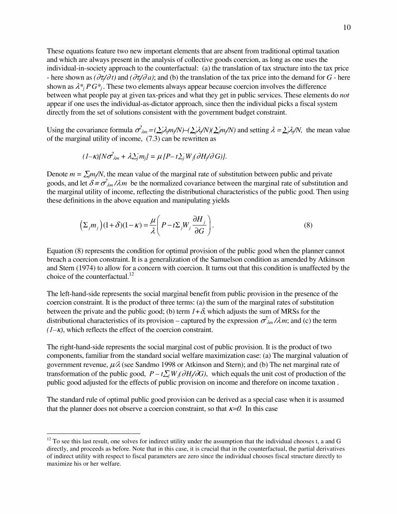
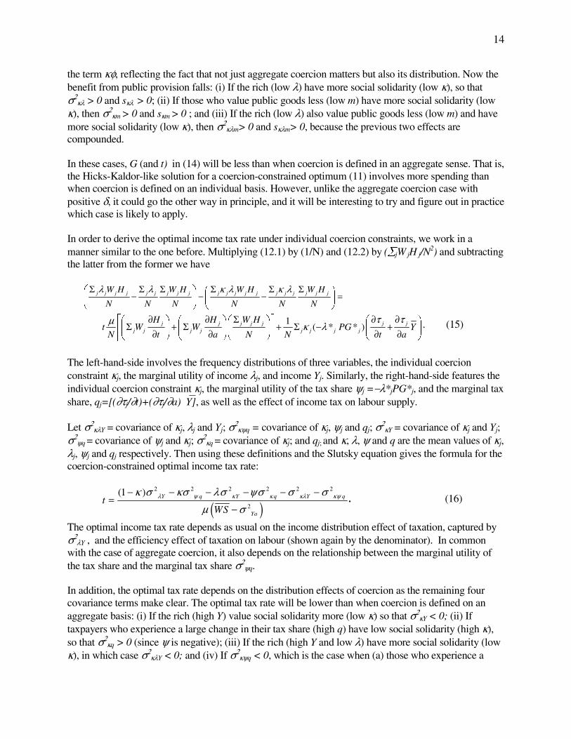
These equations feature two new important elements that are absent from traditional optimal taxation and which are always present in the analysis of collective goods coercion, as long as one uses the individual-in-society approach to the counterfactual: (a) the translation of tax structure into the tax price - here shown as (∂τj/∂ t) and (∂τj/∂ a); and (b) the translation of the tax price into the demand for G - here shown as λ*j P G*j . These two elements always appear because coercion involves the difference between what people pay at given tax-prices and what they get in public services. These elements do not appear if one uses the individual-as-dictator approach, since then the individual picks a fiscal system directly from the set of solutions consistent with the government budget constraint. Using the covariance formula σ2

λm = (∑jλjmj/N)–(∑jλj/N)(∑jmj/N) and setting λ = ∑jλj/N, the mean value of the marginal utility of income, (7.3) can be rewritten as (1–κ)[Nσ2

λm + λ∑j mj] = μ [P– t∑j W j(∂ Hj/∂ G)].

Denote m = ∑jmj/N, the mean value of the marginal rate of substitution between public and private goods, and let δ ≡ σ2

λm /λ m be the normalized covariance between the marginal rate of substitution and the marginal utility of income, reflecting the distributional characteristics of the public good. Then using these definitions in the above equation and manipulating yields

( ) (1 )(1 ) jj j j j

Hm P t W

G

μδ κλ

∂⎛ ⎞Σ + − = − Σ⎜ ⎟∂⎝ ⎠

.

(8)

Equation (8) represents the condition for optimal provision of the public good when the planner cannot breach a coercion constraint. It is a generalization of the Samuelson condition as amended by Atkinson and Stern (1974) to allow for a concern with coercion. It turns out that this condition is unaffected by the choice of the counterfactual.12 The left-hand-side represents the social marginal benefit from public provision in the presence of the coercion constraint. It is the product of three terms: (a) the sum of the marginal rates of substitution between the private and the public good; (b) term 1+δ, which adjusts the sum of MRSs for the distributional characteristics of its provision – captured by the expression σ2

λm /λ m; and (c) the term (1–κ), which reflects the effect of the coercion constraint. The right-hand-side represents the social marginal cost of public provision. It is the product of two components, familiar from the standard social welfare maximization case: (a) The marginal valuation of government revenue, μ/λ (see Sandmo 1998 or Atkinson and Stern); and (b) The net marginal rate of transformation of the public good, P – t∑j W

j(∂ Hj/∂G), which equals the unit cost of production of the

public good adjusted for the effects of public provision on income and therefore on income taxation . The standard rule of optimal public good provision can be derived as a special case when it is assumed that the planner does not observe a coercion constraint, so that κ=0. Ιn this case

12 To see this last result, one solves for indirect utility under the assumption that the individual chooses t, a and G directly, and proceeds as before. Note that in this case, it is crucial that in the counterfactual, the partial derivatives of indirect utility with respect to fiscal parameters are zero since the individual chooses fiscal structure directly to maximize his or her welfare.

11

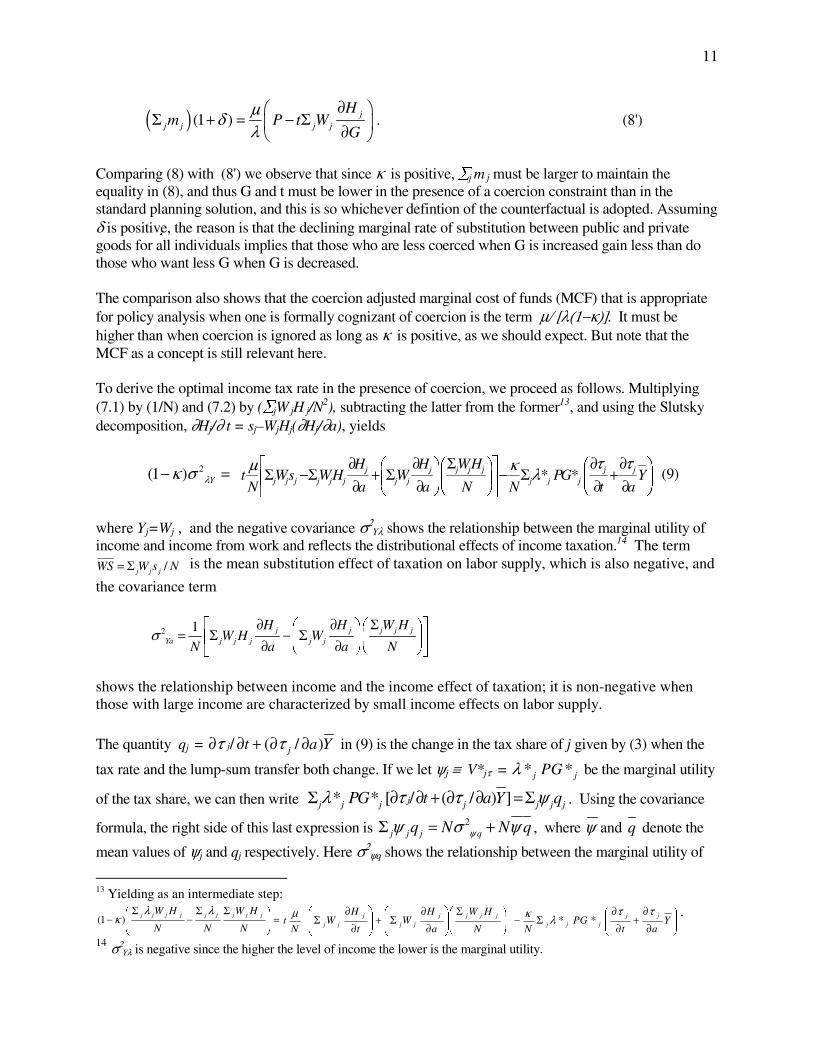
( ) (1 ) jj j j j

Hm P t W

G

μδλ

∂⎛ ⎞Σ + = − Σ⎜ ⎟∂⎝ ⎠

. (8')

Comparing (8) with (8') we observe that since κ is positive, ∑j m

j must be larger to maintain the

equality in (8), and thus G and t must be lower in the presence of a coercion constraint than in the standard planning solution, and this is so whichever defintion of the counterfactual is adopted. Assuming δ is positive, the reason is that the declining marginal rate of substitution between public and private goods for all individuals implies that those who are less coerced when G is increased gain less than do those who want less G when G is decreased. The comparison also shows that the coercion adjusted marginal cost of funds (MCF) that is appropriate for policy analysis when one is formally cognizant of coercion is the term μ/ [λ(1−κ)]. It must be higher than when coercion is ignored as long as κ is positive, as we should expect. But note that the MCF as a concept is still relevant here. To derive the optimal income tax rate in the presence of coercion, we proceed as follows. Multiplying (7.1) by (1/N) and (7.2) by (∑jW

jH

j/N

2), subtracting the latter from the former13, and using the Slutsky decomposition, ∂Hj/∂ t = sj–WjHj(∂Hj/∂a), yields

2(1 ) Yλκ σ− = * *j j j j j j jj j j j j j j j j j j

H H WHt Ws WH W PG YN a a N N t a

τ τμ κ λ∂ ∂ Σ ∂ ∂⎡ ⎤⎛ ⎞⎛ ⎞ ⎛ ⎞Σ −Σ + Σ − Σ +⎢ ⎥⎜ ⎟⎜ ⎟ ⎜ ⎟∂ ∂ ∂ ∂⎝ ⎠⎝ ⎠ ⎝ ⎠⎣ ⎦

(9)

where Yj=Wj , and the negative covariance σ2

Yλ shows the relationship between the marginal utility of income and income from work and reflects the distributional effects of income taxation.14 The term

/j j jWS W s N= Σ is the mean substitution effect of taxation on labor supply, which is also negative, and

the covariance term

2 1 j j j j jYa j j j j j

H H W HW H W

N a a Nσ

⎡ ∂ ∂ Σ ⎤⎛ ⎞⎛ ⎞= Σ − Σ⎢ ⎥⎜ ⎟⎜ ⎟∂ ∂⎝ ⎠⎝ ⎠⎣ ⎦

shows the relationship between income and the income effect of taxation; it is non-negative when those with large income are characterized by small income effects on labor supply.

The quantity qj = / ( / )j jt a Yτ τ∂ ∂ + ∂ ∂ in (9) is the change in the tax share of j given by (3) when the

tax rate and the lump-sum transfer both change. If we let ψj ≡ V*jτ = * *j jPGλ be the marginal utility

of the tax share, we can then write * * [ / ( / ) ]jj j j j j j jPG t a Y qλ τ τ ψΣ ∂ ∂ + ∂ ∂ =Σ . Using the covariance

formula, the right side of this last expression is 2j j j qq N N qψψ σ ψΣ = + , where ψ and q denote the

mean values of ψj and qj respectively. Here σ2ψq shows the relationship between the marginal utility of

13 Yielding as an intermediate step:

=⎟⎟⎠

⎞⎜⎜⎝

⎛ ΣΣ−

Σ−

N

HW

NN

HW jjjjjjjjj λλκ )1( ⎟

⎟⎠

⎞⎜⎜⎝

⎛

∂∂

+∂

∂Σ−

⎥⎥⎦

⎤

⎢⎢⎣

⎡⎟⎟⎠

⎞⎜⎜⎝

⎛ Σ⎟⎟⎠

⎞⎜⎜⎝

⎛

∂∂

Σ+⎟⎟⎠

⎞⎜⎜⎝

⎛

∂∂

Σ Yat

PGNN

HW

a

HW

t

HW

Nt

jj

jjj

jjjj

jj

j

jj

ττλκμ

**.

14 σ2Yλ is negative since the higher the level of income the lower is the marginal utility.

12

the tax share and the marginal tax share15. Also from differentiating the tax share, we have after some work16

0j jj j Y

t a

τ τ∂ ∂Σ = Σ =

∂ ∂, (10)

and thus⎯q = 0. Substituting (10) into (9) and using the definition of σ2

ψq then leads to the coercion-constrained optimal income tax rate:

( )2 2

2

(1 ) Y q

Ya

tWS

λ ψκ σ κσμ σ

− −=

−. (11)

We see that the optimal tax rate is decreasing in the marginal utility of the coercion constraint κ. That is, the less social solidarity or tolerance for coercion, the lower the optimal income tax rate. Given that both σ2

Yλ and the denominator are negative, the optimal tax rate will be lower if σ2ψq is positive; that is, if the

marginal utility of the tax share rises with the tax share. The standard linear optimal tax rate can be obtained as a special case of (11) when κ = 0:

( )2

2

Y

Ya

tWS

λσμ σ

=−

. (11')

By comparing (11) and (11') we see that the more general formulation of the optimal income tax rate features two new terms in comparison to the standard formula: (i) the marginal utility of the coercion constraint, κ ; and (ii) the covariance of marginal utility of the tax share and the marginal tax share, σ2

ψq. 17 Were the individual-as-dictator approach to the counterfactual to be adopted, the optimal tax rate

would then no longer depend on the covariance between the marginal utility of the tax share and the tax share σ2

ψq , since the tax share is not relevant to the definition of that counterfactual.

15 The value of σ2

ψq depends on the size of the parameters of the utility function and is therefore an empirical matter. If tax payers who experience a large increase in their tax shares will also experience a significant fall in utility, σ2

ψq will be negative. 16 Differentiating τj in (3) with respect to the income tax rate t and the lump-sum transfer a, and recognizing that a change in t and a affects the level of income,

2

2

( ) ( ) ( )

( )j Jt j t j t jtt YY Y Y a Y Y at Y Y

t N tY a

∂τ − + − + −=

∂ − and ∂τ

∂j ja j ja j ja a

a

t Y Y Y Y Y Y a Y Y

N tY a=

− + − + −

−

( ) ( )

( )2

where /j jY Y N= Σ is mean income.

Equation (10) follows from these expressions. 17 For completeness, we can contrast this result with the opposite extreme, when the planner must not allow any coercion., i.e. when ∑j (V

*j – Vj ) = 0 . In this case each citizen/consumes the size of the public good which

maximizes his or her utility given their tax share. Attaining such a Lindahl-like solution requires that all individuals consume the same level of the public good. We call this a Lindahl-like solution since taxation is still imposed by the planner rather than representing the result of voluntary exchange.

13

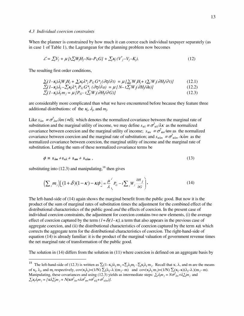
4.3 Individual coercion constraints When the planner is constrained by how much it can coerce each individual taxpayer separately (as in case 1 of Table 1), the Lagrangean for the planning problem now becomes L = ∑jVj

+ μ [t∑jWjHj–Na–PGG] + ∑jκj (V*j –Vj –Kj). (12)

The resulting first order conditions, ∑j(1–κj)λjW

jHj + ∑jκjλ*j PG G*j (∂τj/∂ t) = μ [∑j W

jHj+ t∑j W

j(∂ Hj/∂ t)] (12.1)

∑j(1–κj)λj –∑jκjλ*j PG G*j (∂τj/∂ a) = μ [ N– t∑j W j(∂ Hj/∂a)] (12.2)

∑j(1–κj)λj m j = μ [PG– t∑j W

j(∂ Hj/∂ G)] (12.3)

are considerably more complicated than what we have encountered before because they feature three additional distributions: of the κj, λj, and mj. Like sλm ≡ σ2

λm/λm (≡δ), which denotes the normalized covariance between the marginal rate of substitution and the marginal utility of income, we may define sκλ ≡ σ2

κλ/λκ as the normalized covariance between coercion and the marginal utility of income; sκm ≡ σ2

κm/κm as the normalized covariance between coercion and the marginal rate of substitution; and sκλm ≡ σ2

κλm /κλm as the normalized covariance between coercion, the marginal utility of income and the marginal rate of substitution. Letting the sum of these normalized covariance terms be φ ≡ sλm + sκλ + sκm + sκλm , (13) substituting into (12.3) and manipulating,18 then gives

( ) (1 )(1 )j G jj j

H j

GP t Wm μ

λδ κ κφ

∂

∂

⎛ ⎞⎡ ⎤ = −⎜ ⎟⎣ ⎦ ⎜ ⎟

⎝ ⎠+ − −∑ ∑ . (14)

The left-hand-side of (14) again shows the marginal benefit from the public good. But now it is the product of the sum of marginal rates of substitution times the adjustment for the combined effect of the distributional characteristics of the public good and the effects of coercion. In the present case of individual coercion constraints, the adjustment for coercion contains two new elements, (i) the average effect of coercion captured by the term (1+δ)(1–κ), a term that also appears in the previous case of aggregate coercion, and (ii) the distributional characteristics of coercion captured by the term κφ, which corrects the aggregate term for the distributional characteristics of coercion. The right-hand-side of equation (14) is already familiar: it is the product of the marginal valuation of government revenue times the net marginal rate of transformation of the public good. The solution in (14) differs from the solution in (11) where coercion is defined on an aggregate basis by

18 The left-hand-side of (12.3) is written as ∑j(1–κj)λj m

j =∑jλjmj –∑jκjλj m

j. Recall that κ, λ, and m are the means

of κj, λj, and mj respectively, cov(κjλj)=(1/N) ∑j(λj–λ )(m j– m) and cov(κjλj m

j)=(1/N) ∑j(κj–κ)(λj–λ )(m

j– m).

Manipulating, these covariances and using (12.3) yields as intermediate steps: ∑jλjm j = Nσ2

λm+λ∑jm j and

∑jκjλjm j = [κλ∑jm j + Ν(κσ2

λm+λσ2κm+σ2

κλj+σ2κλm)].

14

the term κφ, reflecting the fact that not just aggregate coercion matters but also its distribution. Now the benefit from public provision falls: (i) If the rich (low λ) have more social solidarity (low κ), so that σ2

κλ > 0 and sκλ > 0; (ii) If those who value public goods less (low m) have more social solidarity (low κ), then σ2

κm > 0 and sκm > 0 ; and (iii) If the rich (low λ) also value public goods less (low m) and have more social solidarity (low κ), then σ2

κλm> 0 and sκλm> 0, because the previous two effects are compounded.

In these cases, G (and t) in (14) will be less than when coercion is defined in an aggregate sense. That is, the Hicks-Kaldor-like solution for a coercion-constrained optimum (11) involves more spending than when coercion is defined on an individual basis. However, unlike the aggregate coercion case with positive δ, it could go the other way in principle, and it will be interesting to try and figure out in practice which case is likely to apply. In order to derive the optimal income tax rate under individual coercion constraints, we work in a manner similar to the one before. Multiplying (12.1) by (1/N) and (12.2) by (∑jW

jH

j/N

2) and subtracting the latter from the former we have

j j j j j j j j j j j j j j j j j j j jW H W H W H W H

N N N N N N

λ λ κ λ κ λΣ Σ Σ Σ Σ Σ⎛ ⎞ ⎛ ⎞− − − =⎜ ⎟ ⎜ ⎟

⎝ ⎠ ⎝ ⎠

1( * * )j j j j j j j

j j j j j j j j

H H W Ht W W PG Y

N t a N N t a

τ τμ κ λ⎡ ∂ ∂ Σ ⎤ ∂ ∂⎛ ⎞ ⎛ ⎞⎛ ⎞ ⎛ ⎞

Σ + Σ + Σ − +⎢ ⎥⎜ ⎟ ⎜ ⎟⎜ ⎟ ⎜ ⎟∂ ∂ ∂ ∂⎝ ⎠ ⎝ ⎠⎝ ⎠ ⎝ ⎠⎣ ⎦

. (15)

The left-hand-side involves the frequency distributions of three variables, the individual coercion constraint κj, the marginal utility of income λj, and income Yj. Similarly, the right-hand-side features the individual coercion constraint κj, the marginal utility of the tax share ψj =−λ*jPG*j, and the marginal tax share, qj=[(∂τj/∂t)+(∂τj/∂a)⎯Y], as well as the effect of income tax on labour supply. Let σ2

κλY = covariance of κj, λj and Yj; σ2κψq = covariance of κj, ψj and qj; σ2

κY = covariance of κj and Yj; σ2

ψq = covariance of ψj and κj; σ2κq = covariance of κj; and qj; and κ, λ, ψ and q are the mean values of κj,

λj, ψj and qj respectively. Then using these definitions and the Slutsky equation gives the formula for the coercion-constrained optimal income tax rate:

( )2 2 2 2 2 2

2

(1 ) Y q Y q Y q

Ya

tWS

λ ψ κ κ κλ κψκ σ κσ λσ ψσ σ σμ σ

− − − − − −=

−. (16)

The optimal income tax rate depends as usual on the income distribution effect of taxation, captured by σ2

λY , and the efficiency effect of taxation on labour (shown again by the denominator). In common with the case of aggregate coercion, it also depends on the relationship between the marginal utility of the tax share and the marginal tax share σ2

ψq. In addition, the optimal tax rate depends on the distribution effects of coercion as the remaining four covariance terms make clear. The optimal tax rate will be lower than when coercion is defined on an aggregate basis: (i) If the rich (high Y) value social solidarity more (low κ) so that σ2

κY < 0; (ii) If taxpayers who experience a large change in their tax share (high q) have low social solidarity (high κ), so that σ2

κq > 0 (since ψ is negative); (iii) If the rich (high Y and low λ) have more social solidarity (low κ), in which case σ2

κλY < 0; and (iv) If σ2κψq < 0, which is the case when (a) those who experience a

15

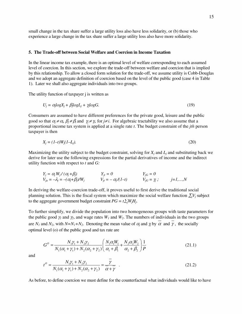
small change in the tax share suffer a large utility loss also have less solidarity, or (b) those who experience a large change in the tax share suffer a large utility loss also have more solidarity. 5. The Trade-off between Social Welfare and Coercion in Income Taxation In the linear income tax example, there is an optimal level of welfare corresponding to each assumed level of coercion. In this section, we explore the trade-off between welfare and coercion that is implied by this relationship. To allow a closed form solution for the trade-off, we assume utility is Cobb-Douglas and we adopt an aggregate definition of coercion based on the level of the public good (case 4 in Table 1). Later we shall also aggregate individuals into two groups. The utility function of taxpayer j is written as Uj = αjlogXj + βjlogLj + γjlogG. (19) Consumers are assumed to have different preferences for the private good, leisure and the public good so that αj ≠ αi, βj ≠ βi and γj ≠ γi, for j≠ i. For algebraic tractability we also assume that a proportional income tax system is applied at a single rate t. The budget constraint of the jth person taxpayer is then Xj = (1–t)Wj(1–Lj). (20) Maximizing the utility subject to the budget constraint, solving for Xj and Lj and substituting back we derive for later use the following expressions for the partial derivatives of income and the indirect utility function with respect to t and G: Yj = αj Wj / (αj +βj) Yjt = 0 YjG = 0 Vja = –λj = –(αj+βj)/Wj Vjt = – αj /(1–t) VjG = γj ; j=1,…,N In deriving the welfare-coercion trade-off, it proves useful to first derive the traditional social planning solution. This is the fiscal system which maximize the social welfare function ∑jVj subject to the aggregate government budget constraint PG = t∑jWjHj. To further simplify, we divide the population into two homogeneous groups with taste parameters for the public good γ1 and γ2, and wage rates W1 and W2. The numbers of individuals in the two groups

are N1 and N2, with N=N1+N2. Denoting the mean value of αj and γj by α and γ , the socially optimal level (o) of the public good and tax rate are

1 1 2 2 1 1 1 2 2 2

1 1 1 2 2 2 1 1 2 2

1

( ) ( )O N N N W N W

GN N P

γ γ α αα γ α γ α β α β

⎛ ⎞+= +⎜ ⎟+ + + + +⎝ ⎠ (21.1)

and

1 1 2 2

1 1 1 2 2 2( ) ( )O N N

tN N

γ γ γα γ α γ α γ

+= =+ + + +

. (21.2)

As before, to define coercion we must define for the counterfactual what individuals would like to have

16

at their given tax-prices. To do so, we maximize utility (19) subject to the budget constraint Wj(1–Lj) = Xj + τjPGj , (20') where the tax share is τj = tYj/ΣjtYj = Wj/ΣjWj . Solving yields

X* j = αjWj; 1− L* j = 1 – βj and * j j j j jj

j

W WG

P P

γ γτ

Σ= = . (22)

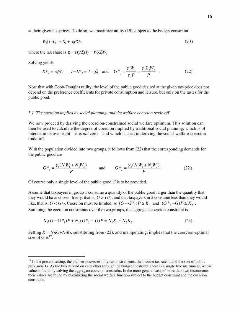
Note that with Cobb-Douglas utility, the level of the public good desired at the given tax-price does not depend on the preference coefficients for private consumption and leisure, but only on the tastes for the public good. 5.1 The coercion implied by social planning, and the welfare-coercion trade-off We now proceed by deriving the coercion-constrained social welfare optimum. This solution can then be used to calculate the degree of coercion implied by traditional social planning, which is of interest in its own right - it is not zero - and which is used in deriving the social-welfare-coercion trade-off. With the population divided into two groups, it follows from (22) that the corresponding demands for the public good are

1 1 1 2 21

( )*

N W N WG

P

γ += and 2 1 1 2 22

( )*

N W N WG

P

γ += . (22')

Of course only a single level of the public good G is to be provided. Assume that taxpayers in group 1 consume a quantity of the public good larger than the quantity that they would have chosen freely, that is, G > G*1, and that taxpayers in 2 consume less than they would like, that is, G < G*2. Coercion must be limited, so 1 1( * )G G P K− ≤ and 2 2( * )G G P K− ≤ .

Summing the coercion constraints over the two groups, the aggregate coercion constraint is 1 1 2 2 1 1 2 2( * ) ( * )N G G P N G G P N K N K− + − = + . (23)

Setting K = N1K1+N2K2, substituting from (22), and manipulating, implies that the coercion-optimal size of G is19:

19 In the present setting, the planner possesses only two instruments, the income tax rate, t, and the size of public provision, G. As the two depend on each other through the budget constraint, there is a single free instrument, whose value is found by solving the aggregate coercion constraint. In the more general case of more than two instruments, their values are found by maximizing the social welfare function subject to the budget constraint and the coercion constraint.

17

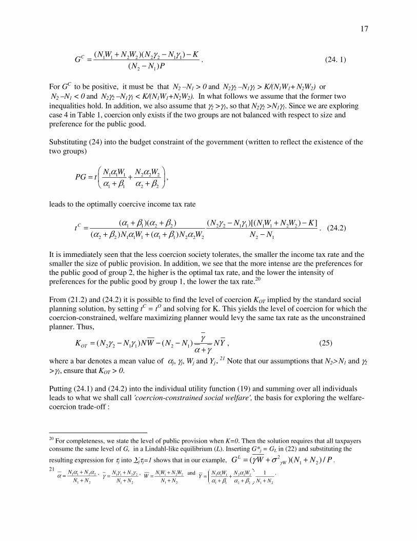
1 1 2 2 2 2 1 1

2 1

( )( )

( )C N W N W N N K

GN N P

γ γ+ − −=−

. (24. 1)

For GC to be positive, it must be that N2 –N1 > 0 and N2γ2 –N1γ1 > K/(N1W1+ N2W2) or N2 –N1 < 0 and N2γ2 –N1γ1 < K/(N1W1+N2W2). In what follows we assume that the former two inequalities hold. In addition, we also assume that γ2 >γ1, so that N2γ2 >N1γ1. Since we are exploring case 4 in Table 1, coercion only exists if the two groups are not balanced with respect to size and preference for the public good. Substituting (24) into the budget constraint of the government (written to reflect the existence of the two groups)

1 1 1 2 2 2

1 1 2 2

N W N WPG t

α αα β α β

⎛ ⎞= +⎜ ⎟+ +⎝ ⎠

,

leads to the optimally coercive income tax rate

1 1 2 2 2 2 1 1 1 1 2 2

2 2 1 1 1 1 1 2 2 2 2 1

( )( ) ( )[( ) ]

( ) ( )C N N N W N W K

tN W N W N N

α β α β γ γα β α α β α

+ + − + −=+ + + −

. (24.2)

It is immediately seen that the less coercion society tolerates, the smaller the income tax rate and the smaller the size of public provision. In addition, we see that the more intense are the preferences for the public good of group 2, the higher is the optimal tax rate, and the lower the intensity of preferences for the public good by group 1, the lower the tax rate.20 From (21.2) and (24.2) it is possible to find the level of coercion KOT implied by the standard social planning solution, by setting tC = tO and solving for K. This yields the level of coercion for which the coercion-constrained, welfare maximizing planner would levy the same tax rate as the unconstrained planner. Thus,

2 2 1 1 2 1( ) ( )OTK N N NW N N NYγγ γ

α γ= − − −

+, (25)

where a bar denotes a mean value of αj, γj, Wj and Yj . 21 Note that our assumptions that N2> N1 and γ2

>γ1, ensure that KOT > 0. Putting (24.1) and (24.2) into the individual utility function (19) and summing over all individuals leads to what we shall call 'coercion-constrained social welfare', the basis for exploring the welfare-coercion trade-off :

20 For completeness, we state the level of public provision when K=0. Then the solution requires that all taxpayers consume the same level of G, in a Lindahl-like equilibrium (L). Inserting G*j = GL in (22) and substituting the

resulting expression for τj into ∑jτj=1 shows that in our example, 21 2( )( ) /L

WG W N N Pγγ σ= + + . 21 1 1 2 2

1 2

N N

N N

α αα +=+

, 1 1 2 2

1 2

N N

N N

γ γγ +=+

, 1 1 2 2

1 2

N W N WW

N N

+=+

and 1 1 1 2 2 2

1 1 2 2 1 2

1N W N WY

N N

α αα β α β

⎛ ⎞= +⎜ ⎟+ + +⎝ ⎠

.

18

1 1 2 2 1 1 1 2 2 2 1 1 2 2( ) ( ) log(1 ( )) log log ( ) logCS K A N N t K N W N W N N Gα α α α γ γ= + + − + + + + (26)

where 1 1 1 1 1 1 1 1 1 2 2 2 2 2 2 2 2 2[ log log ( )log( ) ] [ log log ( )log( )]A N Nα α β β α β α β α α β β α β α β= + − + + + + − + + .

Differentiating (26) with respect to K shows that the trade-off between S and K is concave with an inflection point at K = KOT: 22

( ) 0OT

dSK K

dK

Β= − >Π

for OTK K> (27.1)

and

2

20

d S

dK

Β= − <Π

, (27.2)

where 2 2

1 1 2 2 1 1 1 2 2 2( ) ( ) [ ( ) ( )] 0N Nα β α β α γ α γΒ = + + + + + > , and 2 2

2 1 2 2 1 1 1 2 2 2 1 1(1 )( ) [( ) ( )] 0C Ct t N N N W N Wα β α α α βΠ = − − + + + > .

The trade-off is illustrated in Figure 3, where coercion-constrained welfare is shown on the vertical axis and the given degree of aggregate coercion is on the horizontal. The Appendix shows that the trade-off is the same if the individual-as-dictator counterfactual is used to define the coercion. Of course different patterns of numbers of individuals and of tastes will result in a different trade-off curve. But we stress that it is in principle possible to derive the trade-off using the methodology outlined above.

[Figure 3 here] The figure records that coercion-constrained social welfare is increasing in K for K < KOT. Intuitively, starting from low levels of coercion, the higher the coercion allowed, the easier it is for the planner to implement traditional social planning. This upward sloping part of the locus defines what we may call the 'consenting society'. Points in this region inside the curve represent combinations of coercion and welfare that are not Pareto-efficient. Coercion-constrained welfare reaches a maximum where K = KOT, where the solutions for constrained and unconstrained planning are equal. Finally, coercion-constrained welfare is decreasing for values K > KOT. For levels of coercion higher than KOT the income tax rate falls below its Optimal Tax size, as seen from (24.2), 22 Proof of equations (27): Differentiation of S(K) yields 1 1 2 2 1 1 2 2( )

1

C CN N N NdS dt dG

dK t dK G dK

α α γα γ− + += +−

Substituting from (24.1) and (24.2) into tC and GC and noting that upon differentiation

1 1 2 2

2 2 1 1 1 1 1 2 2 2 1 2

( )( )

[( ) ( ) ]( )

Cdt

dK N W N W N N

α β α βα β α α β α

− + +=+ + + −

and 1 2

1

( )

CdG

dK N N P

−=−

, we have

1 1 2 2 1 1 2 2 1 1 2 2

2 2 1 1 1 1 1 2 2 2 2 1 2 2 1 1 1 1 2 2

( )( )( ) ( )

(1 )[( ) ( ) )]( ) ( )( )C

N N N NdS

dK t N W N W N N N N N W N W K

α α α β α β γ γα β α α β α γ γ

+ + + += −− + + + − − + −

.

Manipulating and using the definition of KOT in (25), the numerator is written as

1 1 2 2 1 1 1 2 2 2( )( )[ ( ) ( )]( )OTN N K Kα β α β α γ α γ+ + + + + − .

Using the definition of tC in (24.1) and manipulating, the denominator is written as 2 2

2 1 2 2 1 1 1 2 2 2 1 1

1 1 2 2

(1 )( ) [( ) ( )]

( )( )

C Ct t N N N W N Wα β α α α βα β α β

− − + + ++ +

. Substituting back into dS/dK yields equations (27). QED.

19

dragging down the level of social welfare. The downward sloping part of the trade off is thus appropriately labelled the 'masochistic society'. If coercion is of vital concern, it is desirable for society to locate on the upward segment of the curve, and not at the peak of the trade-off. Exactly where depends on the degree of coercion, which is not determined here. The analysis here shows that this unsolved problem is of central importance in public economics when the coercion in the life of the community is acknowledged. 23 But even without knowing K, it is still possible to conduct formal analysis of the structure of public policy. One can delineate the trade-off, and ask what policies look like if they are consistent with attainment of the coercion-welfare frontier, as we have done in the previous section by analyzing a fiscal system with a public good financed by a linear income tax. In the Appendix we reformulate the Ramsey Rule (1927) for the structure of commodity taxation, where it is shown that even when cross-elasticities are ignored, tax rates now depend not merely on own-price elasticities, but also on the distribution of tastes for the taxed goods, since the extent of coercion depends on the difference between what citizens receive and what they pay in taxes. 6. Conclusion

Although coercion is a central fact in the operation of the public sector, normative public economics based on the planning model has not made it an explicit element of the analysis. The coercive nature of collective choice has received much attention in the literature that links economics to political processes. Yet, work in this tradition has focused primarily on the design of public choice mechanisms and does not provide a normative framework for comparing and ranking collective choice procedures in relation to the degree of coercion. In this paper, we formally introduce coercion into normative analysis by adding constraints that limit allowable coercion caused by tax and expenditure programs. We focus on what we call “collective goods coercion”, a problem that arises when citizens experience a mismatch between what they receive in public goods and services and what they pay in taxes. While we make use of a methodology that is similar to that employed in optimal taxation, maximizing social welfare subject to coercion constraints, the focus of the analysis is quite different. Optimal taxation asks, given a consensus on the welfare function, what is the best public decision? Here, in view of the absence of consensus about how the collectivity should conduct its affairs, we ask about the trade-off between social welfare and coercion that must occur as a consequence of collective choice. Our intent is to explore the grammar and logic of the analysis when coercion, as distinct from redistribution, is formally and explicitly acknowledged. One should note that the traditional planning model does incorporate the analysis of income redistribution, which may have a coercive aspect. However, it places no formal limits on the extent to which any one individual can be coerced when the social plan is implemented. Furthermore, distributional policies are only one possible source of coercion and differ in nature from public goods coercion which stems from the character of public goods and from the lack of a pricing mechanism for such goods as well as from collective choice.

23 The public choice literature contains possible suggestions about how to approach the choice of K. Although not worked out in a quantifiable manner, the analysis of Buchanan and Tullock (1962, chp. 6) of the optimal decision process may serve as a guide An alternative approach to determining K may rely on ideas from the contractarian literature.

20

To make the concept of coercion operational, a counterfactual specifying what individuals regard as appropriate treatment by the public sector is required. This way of proceeding parallels the approach used in defining violations of rights given to citizens in constitutional documents. As is well known, a standard of justice is a prerequisite for determining the extent and nature of any violations of basic rights. We have formulated with some precision several alternative standards of reference: we may formulate the ideal in terms of individual or aggregate utility or, following Breton (1974) and Buchanan (1967), using a convenient approximation that involves a reference level of government expenditures. The aggregate definitions are analogous to the use of the Hicks-Kaldor criterion and impose a less severe constraint on the decision maker than those having an individual basis. Coercion constraints have significant and complex effects on a social plan. When a linear progressive system of taxation is assumed, tax rates and the level of government expenditures in an extended framework will differ from traditional results. When coercion constraints are defined with reference to individuals, they will become higher or lower than in the traditional analysis, depending on the marginal evaluations of coercion and on the covariance of these with tastes for the public good, among other parameters. When the definition of the counterfactual refers to aggregations of individuals, on the other hand, government expenditures and tax rates will be lower than in an optimal tax plan that fails to account for coercion, assuming only that the value of the Lagrange multiplier on the constraint is positive. Little is known at this point about the relevant empirical magnitudes in both cases. The analysis also has significant implications for the marginal cost of funds (MCF), another central concept in public finance. In the case based on the aggregate definition of coercion, for example, the MCF must be amended to incorporate the value placed on relaxation of the coercion constraint. If this valuation is positive as expected and an aggregate definition of the coercion constraint is adopted, the adjusted MCF will be higher than the one determined in a framework that fails to account for public goods coercion. A novel aspect of the analysis relates to the trade-off between social welfare as traditionally defined and coercion. Using a Cobb-Douglas formulation, we derive a trade-off function, as well as the degree of coercion implied by an unconstrained or social plan. The analysis allows us to examine how to achieve the highest level of traditionally defined welfare for a given degree of coercion or, in other words, how to be coercion-efficient. One should note that the term welfare is narrowly defined in this context. If such welfare falls when the coercion constraint is made stricter, we cannot infer that welfare, defined in a broader context, must also fall. The trade-off function between narrowly defined welfare and public goods coercion is shown to be concave at least in a simplified case, with the maximum representing the point of maximum welfare as traditionally defined. A society (or a planner acting on its behalf) will prefer to be on the upward-sloping part of the relationship, a locus of points corresponding to what we have termed “the consenting society”. Extensions are possible is several directions. The analysis of welfare-coercion trade-offs can be used to gain insight into how coercion can be reduced through institutional means. The analysis by Usher (1977) suggests that how the boundary between private and public sectors is drawn matters in this regard, and that the coercion-welfare frontier can be shifted favorably by removing certain types of economic activity from the public sphere, thereby increasing the chance of reaching stable political equilibria. The trade-off could be used to formalize this argument and analyze the optimal scope of the public sector. Federalism or decentralization of the public sector is another way of shifting the

21

trade-off, as suggested in the Introduction. The Tiebout(1956) model certainly is consistent with this sort of reform, and political scientists such as Pennock (1959) have explicitly investigated how federalism and majority rule interact, but the resulting normative economic theory of fiscal federalism that was prompted by Tiebout's paper has not been explicitly concerned with the coercion that precipitates interregional migration. The analysis here suggests how it may be possible to formally integrate coercion into discussion of the optimal assignment of functions in a federation. Finally, we note that the welfare-coercion frontier also provides the basis for extending the analysis to the study of collective choice, by comparing political equilibria under alternative institutional arrangements in terms of their implied trade-offs between welfare and coercion.

22

Appendix

1. Demonstration that the social welfare - coercion trade-off derived in section 5 is unaffected by the choice of the counterfactual Here we adopt the individual-as-dictator counterfactual rather than the individual-in-society perspective. We must first derive what a individual would like if he or she were allowed to decide for everyone the levels of t and G which maximize their own utility function. We maximize the utility function Uj = αjlogXj + βjlogLj + γjlogG with respect to t and G subject to the

government budget constraint t∑jWj[αj Wj / (αj +βj)] = PG. Solving yields jDj

j j

tγ

α γ=

+ and

1

1j j jD

j jj j j

WG

P

γ αα γ γ

=+ −∑

.

The corresponding demands for the public good are 1 1 1 1 2 2 2

11 1 1 2

1

1 1D N W N W

GP

γ α αα γ γ γ

⎛ ⎞= +⎜ ⎟+ − −⎝ ⎠

and 2 1 1 1 2 2 22

2 2 1 2

1

1 1D N W N W

GP

γ α αα γ γ γ

⎛ ⎞= +⎜ ⎟+ − −⎝ ⎠

.

Summing the coercion constraints over the two groups, the aggregate coercion constraint when it just bites is again 1 1 2 2 1 1 2 2( * ) ( * )N G G P N G G P N K N K− + − = + . Setting K = N1K1+N2K2, substituting

from above, and manipulating, implies that the coercion-optimal size of G is

2 2 1 1

2 2 1 1 2 1

1

( )D N N

G Y KN N P

γ γα γ α γ

⎡ ⎤⎛ ⎞= − Σ −⎢ ⎥⎜ ⎟+ + −⎝ ⎠⎣ ⎦

, where 1 1 1 2 2 2

1 21 1

N W N WY

α αγ γ

Σ = +− −

denotes total income

Using the government budget restraint then leads to the optimally coercive income tax rate

2 2 1 1 1 1 2 2

2 1 1 1 2 2

( ) ( )1

( )( )D N N K

tN N Y

γ α γ γ α γα γ α γ

⎛ ⎞+ − += −⎜ ⎟− + + Σ⎝ ⎠

.

As in the text, setting tD = tO, the optimal solution for t under unconstrained social planning, and solving for K, then yields the level of coercion for which the coercion-constrained, welfare maximizing planner would levy the same tax rate as the unconstrained planner:

2 1 1 1 2 2 1 2 2 1

1 1 2 2 1 1 1 2 2 2

( )( )

( )( )[ ( ) ( )]D

N NK Y

N N

α γ α γ α γ α γα γ α γ α γ α γ

+ + + −= Σ+ + + + +

.

To derive the trade-off following the text, we substitute GD and tD into the welfare function consisting of the sum of individual utilities. Differentiating this expression with respect to K shows that the trade-off between S and K is concave with an inflection point at K = KD:

'( ) 0

' D

dS BK K

dK= − >

Π for

DK K> and 2

2

'0

'

d S

dK

Β= − <Π

,

where 2 2

1 1 2 2 1 1 1 2 2 2' ( ) ( ) [ ( ) ( )] 0N Nα γ α γ α γ α γΒ = + + + + + > and 2 2 2 22 1 1 1 2 2' (1 )( ) ( ) ( ) ( ) 0D Dt t N N Yα γ α γΠ = − − + + Σ > .

This again leads to equations (27) in the text.

23

2. Optimally coercive commodity taxation A longstanding problem concerns the relationship between elasticities of demand and the structure of commodity taxation required to minimize the aggregate excess burden of taxation. We re-examine this problem, first solved by Ramsey (1927), when coercion matters. To keep the analysis simple, we assume there are two homogeneous groups j=1, 2 consuming two commodities i = 1, 2, whose prices are P1 and P2. Individual consumption is denoted by Xji. Each taxpayer pays ad-valorem commodity taxes t1 and t2 on each of two consumption goods. The tax revenue collected is returned lump sum to each individual in equal amounts, denoted by R/2. Taxpayer 1 is assumed to pay too much tax in comparison to what he receives and vice versa for taxpayer 2: this is a highly simplified version of case 4 in Table 1, where the desired size of tax payments is equal to R/2. When coercion constraints bind, taxes must be set so that the overpayment made by taxpayer 1 does not exceed a given sum K1 and the underpayment made by taxpayer 2 must not fall below a certain level K2: thus, 1 1 11 2 2 12 1( / 2)t P X t P X R K+ − = and 1 1 21 2 2 22 2( / 2)t P X t P X R K+ − = − .

The planner chooses t1 and t2 to minimize the excess burden of commodity taxation after securing revenue R, subject to the coercion constraints. Denoting the (absolute value of the) price elasticity of demand for i by ei, assuming that it is identical across groups, and ignoring cross-price effects, the total excess burden of the tax is

2 21 1 1 11 21 2 2 2 21 22(1/ 2) ( ) (1/ 2) ( )B e t P X X e t P X X= + + + ,

and the budget constraint of the government is

1 1 11 21 2 2 12 22( ) ( )t P X X t P X X R+ + + = .

Using κ1 and κ2 to denote the relevant multipliers of the coercion constraints, the solution to the problem of minimizing B subject to the government budget restraint and the coercion constraints is in the usual way seen to be:

1 1 11 2 21 2

2 1 12 2 22 1

t w w e

t w w e

μ κ κμ κ κ

+ +=+ +

, (A1)

where wji=Xji/ΣiXji is group j's share of the consumption of commodity j. The standard inverse elasticity formula is obtained as a special case of (16) when κ1=κ2=0. Then

1 2 2 1/ /t t e e= which implies that the more inelastic good must be taxed more heavily.

However, it is now clear from (A1) that this standard result is no longer valid when coercion is taken into account. The optimally coercive commodity tax rate now depends not only on the inverse of the demand elasticity, but also on the level of coercion tolerated by the taxpayers, and this dependence may in turn

24

reverse the standard conclusion and require that the more elastic good must be taxed more heavily. For example, assume e2 > e1 so that the Ramsey formula indicates lower taxation of the elastic good 2, but that the ratio 1 11 2 21 1 12 2 22( ) /( )p w w w wμ κ κ μ κ κ= + + + + (A2)

is lower than the elasticity ratio. Then for coercion-constrained efficiency it must be that t1 < t2 and the more elastic good 2 must now be taxed relatively more highly. Although the actual size of the p-ratio is an empirical issue, one may expect that the higher the budget shares w12 and w22 (the more both people consume good 2), the more likely that the p-ratio is lower than the ratio of elasticities, and therefore that commodity 2 should be taxed more heavily, contrary to the Ramsey formula. Thus even when cross-elasticities are ignored, tax rates in the amended analysis now depend not merely on own-price elasticities, but also on the distribution of tastes for the taxed goods, since the extent of coercion depends on the difference between what citizens receive and what they pay in taxes. The structure of commodity taxation and the nature of social solidarity In order to study more carefully how the nature of the coercion constraints affects the structure of commodity taxation, we can differentiate the first order conditions for excess burden minimization with respect to t1, t2, κ1 and κ2. Solving the resulting system of four equations, we find that24

1 22

1 1 11 22 21 21

1dt X

dK P X X X X=

−, 1 12

2 1 11 22 21 21

1dt X

dK P X X X X=

−

and

2 21

1 2 11 22 21 21

1dt X

dK P X X X X

−=−

, 2 11

2 2 11 22 21 21

1dt X

dK P X X X X

−=−

.

The sign of these derivatives depends on the sign of the expression (X11X22−X21X12). Let us assume that group 1 is the intensive user of commodity 1. Thus,

11 21 12 22/ /X X X X> , which implies that

X11X22− X21X12 > 0. We then have the following two results: (i) 1 1

1 2

0 , 0d t d t

d K d K> > and (ii) 2 2

1 2

0 , 0d t d t

d K d K< < (A3)

We consider only the first set of inequalities in (A3) since the second set are analogous. The derivatives show that when K1 rises, which means that group 1 is coerced more, the optimal coercive tax rate on the commodity which it uses more intensively (commodity 1) rises too. And when K2 rises, which means that group 2 is coerced less, the tax rate on the commodity which the other group uses more intensively rises.

24 The first order conditions are: e1t1P1X1 = μP1X1 + κ1P1X11 + κ2P2X21; e2t2P2X2 = μP2X2 + κ1P1X12 + κ2P2X22; t1P1X11 + t2P2X12 − (R/2) = K1; t1P1X21 + t2P2X22 − (R/2) = K2. Here except for t1, t2, κ1 and κ2 all parameters are assumed fixed. Differentiating these equations with respect to t1, t2, κ1 and κ2 yields: e1P1X1dt1 + 0× dt2 − P1X11dκ1 − P2X21dκ2 = 0; 0×dt1 + e2P2X2dt2 − P2X12dκ1 − P2X22dκ2 = 0; P1X11dt1 + P2X12dt2 + 0×dκ1 + 0×dκ2 = dK1; and, P1X21dt1 + P2X22dt2+ 0×dκ1 + 0×dκ2 = − dK2 .

25

The intuition for this last result is as follows: recall that group 2 gets more than they pay, and that coercion is defined symmetrically for both groups. Hence, when K2 rises, group 2 gets on balance even more than before, which requires that additional taxes be efficiently raised from group 1.

References Atkinson, Anthony B. and Nicholas H. Stern (1974). "Pigou, Taxation and Public Goods". Review of Economic Studies 41, 119 - 128. Atkinson, Anthony, B and Joseph Stiglitz (1980). Lectures on Public Economics. McGraw-Hill. Baumol (2003), "Welfare Economics and the Theory of the State" , in C. Rowley and F. Schneider (eds.). The Encyclopaedia of Public Choice, Kluwer, 610 - 613. Breton , Albert (1974). The Economic Theory of Representative Government. Chicago: Aldine. Breton, Albert. (1996). Competitive Governments: An Economic Theory of Politics and Public Finance. Cambridge University Press, Cambridge. Buchanan, James, M. and Gordon Tullock (1962). The calculus of consent. Logical foundations of constitutional democracy. Ann Arbor, University of Michigan Press. Buchanan, James (1968). The Demand and Supply of Public Goods. Rand McNally Buchanan, James and Roger Congleton (1998). Politics by Principle, Not Interest. Cambridge University Press. Clower, Robert (1967). "A Reconsideration of the Microfoundations of Monetary Theory", Western Economic Journal Dalton, Thomas (1977). "Citizen Ignorance and Political Activity". Public Choice, 85 - 99. Escarrez, D. R. (1967) ' Wicksell and Lindahl: Theories of Public Expenditure and Tax Justice Reconsidered' National Tax Journal 20, 137-148 Hettich, Walter and Stanley L. Winer (1985). " Blueprints and Pathways: The Shifting Foundations of Tax Reform". National Tax Journal. Hettich, Walter and Stanley L. Winer (1999). Democratic Choice and Taxation: A Theoretical and Empirical Investigation. Cambridge University Press. Kaplow, Louis (2005). "Pareto Principles and Competing Principles". The New Palgrave Dictionary of Economics and the Law, 2nd Edition. Forthcoming. (Harvard Law School Discussion paper 519, August 2005). Levy, Margaret (1997). Consent, Dissent, and Patriotism. Cambridge University Press.

26

Lindahl, Eric (1919). "Just taxation, a Positive Solution". in R. Musgrave and A. Peacock (1958). Classics in the Theory of Public Finance. Macmillan 1958, 168-176. Mirrlees, James A. (1971). "An Exploration in the Theory of Optimum Income Taxation," Review of Economic Studies, 38, 175-208. Patinkin, Don (1965). Money, Interest and Prices: An Integration of Monetary and Value Theory. 2nd Edition. Harper and Row. Pennock, Roland (1959). "Federal and Unitary Government - Disharmony and Frustration". Behavioral Science 4. Perroni, Carlo and Kimberley Scharf (2003). "Viable Tax Constitutions". Unpublished, University of Warwick, September. Ramsey, Frank P. (1927). "A contribution to the theory of taxation." Economic Journal 37, 47-61. Sandmo, Agnar (1984). "Some Insights from the New Theory of Public Finance," Empirica 2, 111-124. Sandmo, Agnar (1983). "Progressive taxation, redistribution and labor supply," Scandinavian Journal of Economics 85, 311-323 Sandmo, Agnar (1998). "Redistribution and the marginal cost of public funds" Journal of Public Economics 70, 365-382. Simons, Henry C. (1938). Personal Income Taxation: The Definition of Income as a Problem of Fiscal Policy. University of Chicago Press. Slutsky, Steven M. (1979). ' Equilibrium Under α-Majority Voting'. Econometrica 47, 1113-1125. Usher, Dan. (1977). "The welfare economics of the socialization of commodities". Journal of Public Economics 8, 151-168. Usher, Dan (1993). The Welfare Economics of Markets, Voting and Predation. University of Michigan Press Usher, Dan (1981). The Economic Prerequisites of Democracy. Routledge. Weldon, Jack (1968?) On federalism showing that there is no reason for it in standard theory (you could just as well have administrative decentralization). Wicksell, Knut (1896). "A New Principle of Just Taxation". in R. Musgrave and A. Peacock (1958). Classics in the Theory of Public Finance. Macmillan, 72-118.

Winer, Stanley L. and Hirofumi Shibata editors (2002). Political Economy and Public Finance: The Role of Political Economy in the Theory and practice of Public Economics. Edward Elgar.

27

Wiseman, Jack (1989). Cost and Choice and Political Economy. Edward Elgar Publishing.

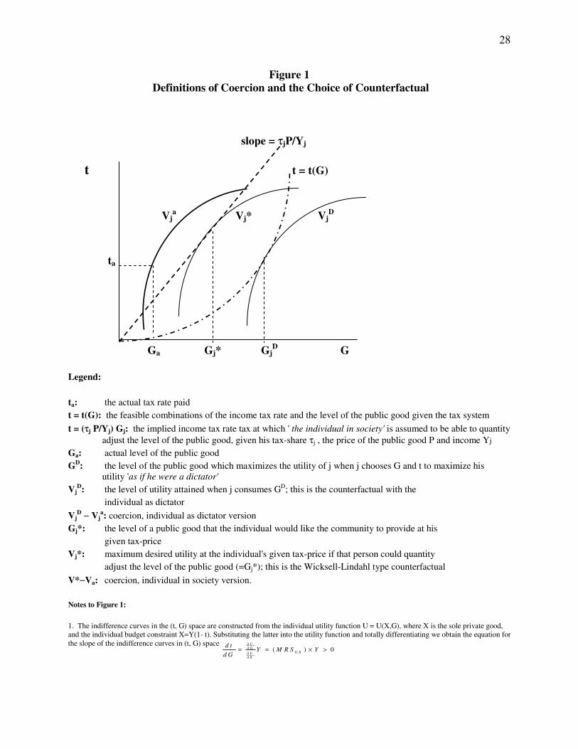
28

Figure 1 Definitions of Coercion and the Choice of Counterfactual

slope = τjP/Yj

t t = t(G) Vj

a Vj* VjD

ta

Ga Gj* GjD G

Legend: ta: the actual tax rate paid t = t(G): the feasible combinations of the income tax rate and the level of the public good given the tax system

t = (τj P/Yj) Gj: the implied income tax rate tax at which ' the individual in society' is assumed to be able to quantity adjust the level of the public good, given his tax-share τj , the price of the public good P and income Yj

Ga: actual level of the public good GD: the level of the public good which maximizes the utility of j when j chooses G and t to maximize his utility 'as if he were a dictator' Vj

D: the level of utility attained when j consumes GD; this is the counterfactual with the individual as dictator

VjD − Vj

a: coercion, individual as dictator version Gj*: the level of a public good that the individual would like the community to provide at his given tax-price Vj*: maximum desired utility at the individual's given tax-price if that person could quantity adjust the level of the public good (=Gj*); this is the Wicksell-Lindahl type counterfactual

V*−Va: coercion, individual in society version. Notes to Figure 1: 1. The indifference curves in the (t, G) space are constructed from the individual utility function U = U(X,G), where X is the sole private good, and the individual budget constraint X=Y(1- t). Substituting the latter into the utility function and totally differentiating we obtain the equation for the slope of the indifference curves in (t, G) space

( ) 0UG

G XUX

d tY M R S Y

d G

∂∂∂∂

= = × >

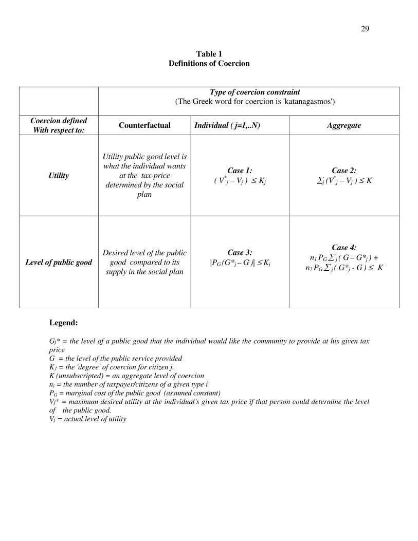
29

Table 1 Definitions of Coercion

Type of coercion constraint

(The Greek word for coercion is 'katanagasmos')

Coercion defined With respect to:

Counterfactual Individual ( j=1,..N) Aggregate

Utility

Utility public good level is what the individual wants

at the tax-price determined by the social

plan

Case 1: ( V*

j – Vj ) ≤ Kj Case 2:

∑j (V*j – Vj ) ≤ K

Level of public good Desired level of the public

good compared to its supply in the social plan

Case 3: |PG (G*j – G.)| ≤ Kj

Case 4: n1 PG ∑ j ( G – G*j ) +

n2 PG ∑ j ( G*j - G ) ≤ K

Legend: Gj* = the level of a public good that the individual would like the community to provide at his given tax price G = the level of the public service provided K j = the 'degree' of coercion for citizen j. K (unsubscripted) = an aggregate level of coercion ni = the number of taxpayer/citizens of a given type i PG = marginal cost of the public good (assumed constant) Vj* = maximum desired utility at the individual's given tax price if that person could determine the level of the public good. Vj = actual level of utility

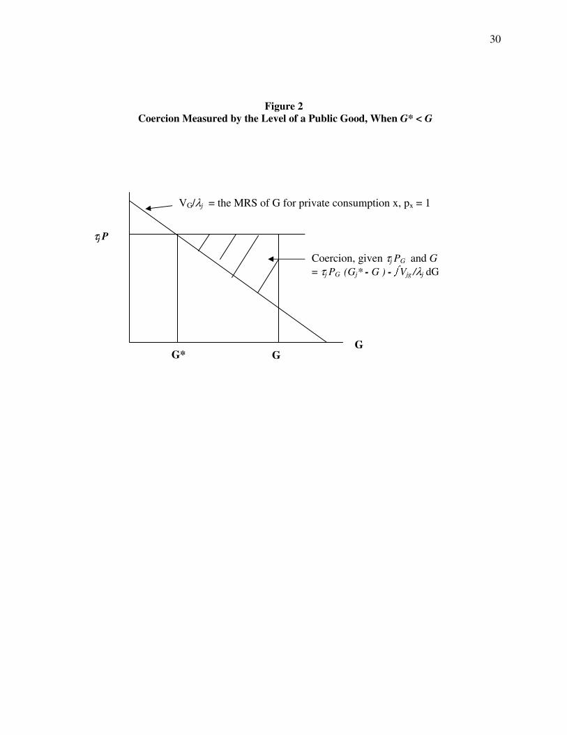
30

Figure 2 Coercion Measured by the Level of a Public Good, When G* < G

G G

VG/λj = the MRS of G for private consumption x, px = 1

τj P

G*

Coercion, given τj PG and G = τj PG (Gj* - G ) - ∫ Vjg /λj dG

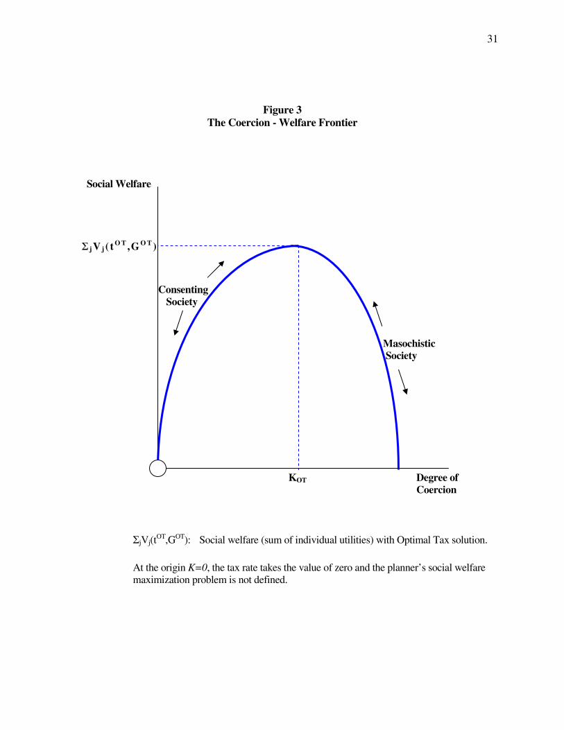
31

Figure 3 The Coercion - Welfare Frontier

Social Welfare Σ j V j ( t O T ,G O T )

Consenting Society

Masochistic Society KOT Degree of Coercion

ΣjVj(tOT,GOT): Social welfare (sum of individual utilities) with Optimal Tax solution.

At the origin K=0, the tax rate takes the value of zero and the planner’s social welfare maximization problem is not defined.