Embed Size (px)
Citation preview

1
Social Norms
Mary A. Burke and H. Peyton Young
This version: April 17, 2009
Forthcoming in The Handbook of Social Economics, edited by Alberto Bisin, Jess Benhabib,
and Matthew Jackson. Amsterdam: North-Holland.
I. Background
Social norms and customs shape many economic decisions, but they have not always
been at the forefront of economic analysis. Indeed, social influences were more
prominently acknowledged by the founders of the discipline than by neoclassical
theorists of the last century. J.S. Mill, for example, argued that custom was a potent
force in setting the terms of contracts and also the wages paid to labor: “[T]he division
of produce is the result of two determining agencies: competition and custom. It is
important to ascertain the amount of influence which belongs to each of these causes,
and in what manner the operation of one is modified by the other…Political economists
in general, and English political economists above others, have been accustomed to lay
almost exclusive stress upon the first of these agencies; to exaggerate the effect of
competition, and to take into little account the other and conflicting principle.” (Mill,
1848, Book II, Chapter IV).
Later, Marshall pointed to the effects of custom on the dynamics of economic
adjustment, suggesting that they would make adjustment sticky and punctuated by
sudden jumps: “The constraining force of custom and public opinion …resembled the

2
force which holds rain-drops on the lower edges of a window frame: the repose is
complete till the window is violently shaken, and then they fall together...” (Marshall,
1920, p. 641).
Unfortunately, the difficulty of making such dynamic arguments precise led to their
being put on the back burner for many years. Meanwhile an opposing view took hold
in which individuals’ choices were treated as if they were mediated only by prices and
self-regarding preferences; norms, customs, and social influences were treated as
secondary effects that could be safely ignored. This position was stated in a particularly
stark form by Frank Knight as one of the pre-conditions for perfect competition: “Every
person is to act as an individual only, in entire independence of all other persons. To
complete his independence he must be free from social wants, prejudices, preferences,
or repulsions, or any values which are not completely manifested in market dealing.”
(Knight, 1921, p.78)
In recent decades there has been a return to the earlier point of view, which
acknowledges that individual choices are mediated by norms, customs, and other forms
of social influence. The aim of this chapter is to provide an overview of recent work
that shows how to incorporate norms into economic models, and how they affect the
dynamics of economic adjustment. Given space limitations it is impossible to do justice
to the many varied ways in which norms have been modeled in the recent literature; 1
instead, we shall focus on a trio of models that illustrate the approach in three different
settings: contractual norms in agriculture, norms of medical practice, and body weight
norms. While the specific mechanisms of norm enforcement differ across these cases, it
turns out that certain qualitative features of the dynamics cut across many different
applications, just as Marshall suggested.
1 Contributions that we will not have space to consider in detail include Akerlof (1980, 1997), Becker and Murphy (2000), Bicchieri (2006), Coleman (1987), Elster (1989), Hechter and Opp (2001), Lewis (1969), Schotter (1981), and Ullman-Margalit (1977). For a survey of modeling and identification issues in the presence of social interactions see Durlauf and Young (2001).

3
II. Norms, customs, and conventions
We define a social norm as a standard, customary, or ideal form of behavior to which
individuals in a social group try to conform. We do not believe it is fruitful to draw a
distinction between norms and conventions, as some authors have tried to do. In our
view there is no simple dichotomy between the two concepts, based for example on
whether or not the behavior is enforced by third parties. We would argue that there is a
constellation of internal and external mechanisms that hold norms in place, and that the
salience of these factors varies from one situation to another. In some societies, for
example, it is a norm to avenge an insult. A person who is insulted and does not
avenge his honor will lose social status and may be severely ostracized. In this case the
norm is held in place by third-party sanctions.2 However, consider the norm against
littering in public areas. People are often in a situation where they can litter without
being observed, nevertheless they may refrain from doing so because they would not
think well of themselves. In this case the norm is held in place by an internalized sense
of proper or moral conduct.
As a third example, consider the norm of extending the right hand in greeting. This
solves a simple coordination problem: there is no need for third party enforcement or
internalized codes of conduct. Thus one might say it is “merely” a convention, but this
distinction is not particularly useful, because the desire to conform may be just as
strong for conventions as for norms. Furthermore, adhering to convention does more
than solve a coordination problem, it signals one’s attentiveness to the nuances of social
interaction. Extending one’s left hand would not only cause a momentary coordination
failure, it would raise questions about what the act might mean.
2 Experimental evidence suggests that subjects are willing to punish norm violators even at some cost to themselves (Fehr, Fischbacher, and Gaechter, 2002; Fehr and Fischbacher, 2004a,b).

4
We prefer, therefore, to view social norms as encompassing both conventions and
customs, and not to draw fine distinctions between them according to the mechanisms
that hold them in place. The key property of a social norm from a modeling standpoint
is that it induces a positive feedback loop in behaviors: the more widely that a norm is
followed by members of a social group, the more everyone wants to adhere to it.
In its simplest form, this type of feedback loop can be modeled by a coordination game.
Suppose that members of a group interact randomly and in pairs, and that each
interaction involves playing a coordination game with two actions: Left and Right. A
norm is a situation in which the population in general plays one or the other, and
everyone has come to expect this. In other words, a social norm corresponds to a pure
equilibrium of a coordination game that is played repeatedly by members of a
population, with the proviso that the equilibrium is not conditional on who is playing.
Note that this framework can be extended to include more complex games in which the
equilibrium involves punishments for deviation. The relevant point is that the
equilibrium holds at the population level, inducing common expectations and behaviors
for an interaction that is repeated over time by members of a social group. The
framework can be extended still further by incorporating both individual and
interactive terms into the analysis. In other words, an agent’s utility may derive in part
from his idiosyncratic preference for a particular action, and in part from the extent to
which the action dovetails with the actions of others. This set-up allows one to explore
the interaction between positive feedback loops due to social norms, and (possibly
negative) feedback loops induced by competing demands for ordinary consumption
goods.
III. Characteristic features of norm dynamics

5
Before turning to specific applications, however, we wish to draw attention to certain
characteristic features of models in which social norms play a role. We shall single out
four such features: local conformity/global diversity, conformity warp, punctuated
equilibrium, and equilibrium stability. We briefly discuss these features below without
specifying the models in detail; these will be considered in subsequent sections.
Local conformity/global diversity
When agents interact in a social group and there are positive feedback effects from their
behaviors, there will be a tendency for the population to converge to a common
behavior, which can be interpreted as a social norm. Frequently, however, there are
alternative behaviors that can form an equilibrium at the population level (e.g., different
coordination equilibria in a pure coordination game), so there is indeterminacy in the
particular social norm that will eventually materialize. Suppose that society is
composed of distinct subgroups or “villages” such that social interactions occur within
each village but not between them. Starting from arbitrary initial conditions, different
villages may well end up with different norms. That is, there will be near-uniformity
of behavior within each village, and substantially different behaviors across villages.
This is the local conformity/global diversity effect. It turns out that this effect is present
even when society is not partitioned into distinct villages: it suffices that ties across
subgroups are relatively weak, or that the strength of interactions falls off with
geographic (or social) distance. This effect is discussed in two of our case studies: the
choice of agricultural contracts and the choice of medical practices, where in both cases
the effect has strong empirical support.
Conformity warp
When social interactions are not present, agents usually optimize based on their
personal preferences, that is, their actions are determined by their “types.” For example,

6
people vary considerably in their natural body weights, depending on genetic
inheritance and other factors including age, education level, and idiosyncratic
preferences. Absent social norms, weight would be determined solely by such
individual factors, together with economic constraints such as food prices. If, however,
a social norm about appropriate or desirable body weight is in force within a group, its
members will try to conform to the norm, which implies that some people make choices
that are warped away from the choices they would make if there were no norm.
Testing for this effect empirically is complicated by the fact that the “warp” could arise
from some unobserved common factor rather than from a social norm. For example, in
a region in which food prices are low based on supply-side reasons, people will tend to
be heavier than they would in an environment with more expensive food. While it may
be possible to control for food prices, other common factors may be unknown or
unobservable. However, if there is an observable exogenous factor that affects individual
weight, such as a genetic marker, one can use the group prevalence of that factor as an
instrument for the group’s average weight and test for an influence of the predicted
average weight on individual weight, controlling for the genetic marker at the
individual level. If social body weight norms are operative, the weights of those in the
genetic minority will be warped away from what would be predicted on the basis of
their genetic type, towards the size predicted by the group’s average genetic makeup.3
We first identified this warping effect in connection with the choice of agricultural
contracts (Young and Burke, 2001). In that setting, a natural predictor of contract choice
(absent social effects) is the soil quality on a given farm. (Higher soil qualities produce
naturally higher yields, which should be reflected in improved terms for the
landowner.) What we find, however, is that contract choice is remarkably uniform
across farms with different soil qualities that are located in the same region (a regional
3 For this to be a valid instrument, the group average trait must have no direct effect on the individual, controlling for her own trait, and must not predict other, unobserved individual traits that affect weight.

7
norm). Moreover, the terms of a regional norm correspond more or less to the average
soil quality within that region. Consequently, regional outliers (farms with
exceptionally low or high soil quality for that region) tend to have contracts whose
terms differ substantially from the terms that would hold if they were the only farms (or
if social interactions were not present). A similar phenomenon arises in regional
variations in medical treatment, as we discuss in the second case study below.
Punctuated equilibrium
One consequence of increasing returns is that a social norm, once established, may be
quite difficult to dislodge even when circumstances change. In particular, incremental
changes in external conditions (e.g., prices) may have no effect, because they are not
large enough to overcome the positive feedback effects that hold the norm in place. In
short, it may take a very large change in conditions before a norm shift is observed,
which is precisely the effect to which Marshall was referring in his raindrops example.
A second way in which norms can shift is through the accumulation of many small
changes in behaviors. The process is analogous to mutation: suppose that, by chance,
some doctors in a particular region happen to experiment with a new procedure. Their
experience will rub off on their colleagues, who may then be more inclined to try it than
they otherwise would be. If enough of these (positive) experiences accumulate, a
tipping point is reached in which an existing treatment norm is displaced in favor of a
new one. Note that, unlike an exogenously-induced norm shift, this type of shift will
appear to be spontaneous.
Equilibrium stability

8
The incorporation of stochastic shocks into the dynamic adjustment process leads to the
striking prediction that some norms are much more likely than others to be observed
over the long run. The reason is that the likelihood of norm displacement, due to an
accumulation of small stochastic shocks, depends on the “depth” of the basin of
attraction in which the norm lies. This fact can be exploited to estimate the probability
that different norms will be observed in the long run, using techniques from the theory
of large deviations in stochastic dynamical systems theory (Freidlin and Wentzell, 1984,
Foster and Young, 1990, Young, 1993a, Kandori, Mailath, and Rob, 1993). Moreover
when the shocks have very small probability and are independent across actors, the
theory shows that only a few norms (frequently a unique norm) will have nonnegligible
long-run probability. These norms are said to be stochastically stable (Foster and Young,
1990).
This effect is discussed in some detail in our case study on contractual norms in
agriculture. Here the theory makes two specific predictions: i) contractual terms will
tend to be locally uniform even though there is substantial heterogeneity in the quality
of the inputs (labor and land), which in neoclassical theory would call for similar
heterogeneity in the contracts, and ii) contractual terms may differ markedly between
regions, with sharp jumps observed between neighboring regions, rather than more or
less continuous variation.
IV. Social interactions and social norms
Models involving social interactions have proved particularly useful in capturing a
variety of phenomena that exhibit local uniformity, together with diversity in average
behavior across regions or groups that exceeds the variation in fundamentals across
such units. The framework constitutes a tractable and powerful way to describe
variation in social norms across societies and over time—allowing for considerable
within-group heterogeneity—where the distribution of behaviors and the social norm

9
exhibit mutual causality. A social interaction occurs when the payoff to an individual
from taking an action is increasing in the prevalence of that action among the relevant
set of social contacts. As we illustrate in three examples below, the choice model is not
a pure coordination game. Rather, agents trade off private incentives against social
rewards or penalties, and conformity may be incomplete. Interactions may be either
local or global—in the latter case, agents optimize against the mean action of the entire
population, whereas in the former the social interaction occurs only with a local subset
of the population. The assumption that agents benefit from behaving similarly to
others—an example of strategic complementarity—gives rise to a social multiplier, such
that the effect of variation in fundamentals is amplified in the aggregate relative to a
situation involving socially isolated choices.4
Social interactions may accelerate shifts in social norms over time initiated by
technological change and other shocks—that is, interactions may lead to punctuated
equilibria. For example, Goldin and Katz (2002) link the birth control pill, via direct
effects as well as indirect, social multiplier effects, to the dramatic increases in women’s
career investment and age of first marriage in the 1970s. Contraception has also been
linked to the large increases in out-of-wedlock births since the 1960s (Akerlof, Yellen
and Katz, 1996), where the technology’s direct impact eventually served, via social
interactions, to erode the social stigma against out-of-wedlock births. As shown below,
there is evidence that social multiplier effects have magnified the impact of falling food
prices on obesity rates in the United States in recent decades and led to a larger value of
the social norm for body size (Burke and Heiland, 2007).
V. A model of norm dynamics
4 Canonical models of social interactions are provided by Brock and Durlauf (2001) Becker and Murphy (2000), and Glaeser and Scheinkman, 2003). See Burke (2008) and Glaeser, Sacerdote, and Scheinkman (2003) for a further discussion of social multipliers.

10
We turn now to the question of how social norms arise in the first place. If they
represent equilibrium behaviors in situations with multiple equilibria, how does society
settle on any particular one starting from out-of-equilibrium conditions? To model this
situation, imagine a population of players who interact over time, where each
interaction entails playing a certain game G . For expositional simplicity we shall
assume that G is a two-person game; the general framework extends to the n-person
case. We shall make the following assumptions:
i) Players do not necessarily know what is going on in the society at large; their
information may be local, based on hearsay, or on personal experience.
ii) Players behave adaptively -- for the most part they choose best replies given
their current information;
iii) Players occasionally deviate from best responses for a variety of unmodeled
reasons; we represent these as stochastic shocks to their choices.
iv) Players interact at random, though possibly with some bias toward their
geographical or social “neighbors.”
We wish to examine how behaviors evolve in such a population over time starting
from arbitrary initial conditions. In particular, we would like to know whether
behaviors converge to some form of population equilibrium (a social norm), and, if
so, whether some norms are more likely to emerge than others.
To be concrete, let us assume that G is a symmetric two-person coordination game,
where each player chooses an action from a finite set X . Given a pair of actions,
( , )x x , denote the payoff to the first player by ( , )u x x , and the payoff to the second

11
player by ( , )u x x . We assume that each of the pairs ( , )x x is a strict Nash
equilibrium of the one-shot game.
Now consider a population of n players who interact pairwise. The “proximity” of
two players i and j is given by a weight 0ijw , where we assume that ij jiw w .
We can think of ijw as the relative probability that two players will interact, or the
importance of their interaction, or some combination thereof.
Consider a discrete-time process with periods 1,2,3,....t At the end of period t ,
the state of the system is given by an n -vector ( )tx , where ( )ix t X is the current
strategy choice by player i , 1 i n . The state space is denoted by nXX . Assume
that players update their strategies asynchronously: at the start of period 1t , one
agent is chosen at random to update. Call this agent i . Given the choices of
everyone else, which we denote by ( )i tx , the expected utility of agent i from
choosing action x is defined to be
,
( , ( )) ( , ( ))i i ij ji j
U x t w u x x t x .
Assume that i chooses a new action ( 1)ix t x with a probability that is
nondecreasing in its expected utility, where all actions have a positive probability of
being chosen. A particularly convenient functional form is the logistic response
function
( , ( )) ( , ( ))[ ] /i i i iU x t U x ti
x S
P x x e e
x x .
This is also known as a log-linear response function, because the difference in the log-
probabilities of any two actions is a linear increasing function of the difference in

12
their expected payoffs. [Blume, 2003; Young, 1998a]. This is a standard
representation of discrete choice behavior, and can be justified as a best-response
function when an agent’s utility is subjected to a random utility shock that is
extreme-value distributed [Mcfadden, 1974; Durlauf, 1997; Brock and Durlauf, 2001].
This adjustment rule is convenient to work with because the Markov learning
process has a stationary distribution that takes an especially simple form. Define the
potential function : R X such that for every state x X ,
,
( ) ( , )ij i ji j
w u x x x .
Theorem. The unique stationary distribution of the Markov learning process is
( ) ( )( ) /e e
x x
x X
x , (1)
that is, from any initial state, the long-run frequency of state x is ( ) x .
Corollary. When is high (agents best-respond with high probability), the state(s)
that maximize potential are the most probable, and when is very large the
state(s) that maximize potential have probability close to one. These are known as
the stochastically stable states of the evolutionary process [Foster and Young, 1990].
Many variants of this approach have been discussed in the literature. One variation
is to suppose that each agent reacts to a random sample of current (or past) choices
by other agents (Young, 1993a, 1998). This captures the idea that agents typically
have limited information based on personal experience and local contacts. Other
variations are obtained by assuming that deviations from best response follow a

13
distribution that differs from the logistic. For example, one could assume that all
non-best response strategies are chosen with equal probability (mutations are purely
random). Under this assumption the long-run dynamics cannot be expressed in a
simple closed form such as (1); nevertheless it is reasonably straightforward to
characterize the states that have high probability in the long run (Young, 1993a).
The evolutionary approach can also be adapted to non-symmetric games involving
two or more players. Given an n -person game G , assume that the population can
be divided into n disjoint subpopulations, one for each “role” in the game. In each
period a set of n individuals is selected at random, one from each subpopulation,
and they play G . As in the previous models, each agent best-responds with high
probability to an estimate of the frequency distribution of choices by other agents
(Young, 1993a).
Different stochastic adjustment rules can yield different predictions about the
specific equilibria that are most likely to emerge over the long run. These are known
as the stochastically stable equilibria of the evolutionary process.5 For certain
important classes of games, however, the predictions are reasonably consistent
across a wide range of modeling details. We mention two such results here.
A two-person game G is a pure coordination game if each player has the same number
of strategies, and the strategies can be indexed so that it is a strict Nash equilibrium
to match strategies, i.e., when one player uses his thk strategy, the other’s unique
best response is her thk strategy. Note that this definition does not presume that the
players’ strategies are the same, or that they have the same payoff functions.
5 This term was introduced by Foster and Young (1990) and can be stated quite generally as follows: a state of a perturbed Markov chain is stochastically stable if its long-run probability is bounded away from zero for arbitrarily small perturbations.
14
A natural example of such a game arises when players must first agree on the rules
of the game. Consider, for example, a two-person interaction in which the rules can
take m different forms. Before they can interact, the players must agree on the rules
that will govern their interaction. If they agree on the thk set of rules, they play the
game and get the expected payoffs ( , )k ka b . If they fail to agree their payoffs are
zero. Assume that all versions of the game are worth playing, that is, , 0k ka b for
all k . This is a pure coordination game. A population-level equilibrium in which
everyone plays by the same set of rules can be viewed as a social norm. It can be
shown that, under a fairly wide range of stochastic best response rules, such a
process will select an efficient norm: an equilibrium whose payoffs are not strictly
dominated by the payoffs in some alternative equilibrium [Kandori and Rob, 1995;
Young, 1998b].6
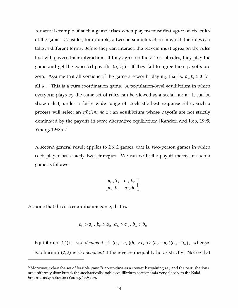
A second general result applies to 2 x 2 games, that is, two-person games in which
each player has exactly two strategies. We can write the payoff matrix of such a
game as follows:
11 11 12 12
21 21 22 22
, ,
, ,
a b a b
a b a b
Assume that this is a coordination game, that is,
11 21 11 12 22 12 22 21, , , a a b b a a b b
Equilibrium (1,1) is risk dominant if 11 21 11 12 22 12 22 21( )( ) > ( )( )a a b b a a b b , whereas
equilibrium (2,2) is risk dominant if the reverse inequality holds strictly. Notice that
6 Moreover, when the set of feasible payoffs approximates a convex bargaining set, and the perturbations are uniformly distributed, the stochastically stable equilibrium corresponds very closely to the Kalai-Smorodinsky solution (Young, 1998a,b).

15
this definition coincides with efficiency if the off-diagonal payoffs are zero (as in a
pure coordination game), but otherwise risk dominance and efficiency may differ. It
can be shown that, under fairly general assumptions, the risk dominant equilibrium
is stochastically stable in an evolutionary process based on perturbed best responses
[Blume, 2003].
Although evolutionary models of norm formation differ in certain details, they have
several qualitative implications that hold under a wide range of assumptions.
Assume that a given type of interaction can be represented as a coordination game
in which the alternative equilibria correspond to different potential norms. Assume
also that the evolutionary process is based on random interactions with some form
of perturbed best responses by the agents. Under quite general conditions, a given
population or “society” will eventually find its way toward some equilibrium; in
other words, a social norm will become established with high probability. Within
such a society there will be a high degree of uniformity in the way that people
behave (and expect others to behave) in this type of interaction, though there may
not be perfect uniformity due to the presence of idiosyncratic behaviors (mutations).
Second, different societies (or subgroups that have limited interactions with one
another) may arrive at different norms for solving the same type of coordination
problem, due to chance events and the vagaries of history. Putting these two
phenomena together, we can say that social norms lead to a high degree of
conformity locally (within a given society), and possibly much greater diversity
globally (among societies). This is known as the local conformity/global diversity effect
(Young, 1998a).
Another general phenomenon predicted by evolutionary models is that social norms
can spontaneously shift due to stochastic shocks. Such shifts may be precipitated by
an accumulation of small changes in behaviors and expectations (mutations), by an
external shock that suddenly changes agents’ payoff functions, or by some form of

16
coordinated action (e.g., a social movement). The theoretical models discussed
above focus on the effect of small chance events, but the other two mechanisms are
certainly important in practice. A common implication of all of these mechanisms,
however, is that shifts will tend to be very rapid once a certain threshold is crossed.
The reason is that the linkage between expectations and behaviors induces a highly
nonlinear feedback effect: if enough people change the way that they do things (or
they way they expect others to do things) everyone wants to follow suit, and the
population careens toward a new equilibrium. In other words, once a norm is in
place it tends to remains so for a long time, and shifts between norms tend to be
sudden rather than gradual . This is known as tipping or the punctuated equilibrium
effect (Young, 1998a).7
VI. Contractual norms in agriculture
The framework outlined above has potential application to any situation in which social
norms influence agents’ decisions. Relevant examples include the use of addictive
substances, dropping out of school, and criminal behavior [Case and Katz,1991; Crane,
1991; Glaeser, Sacerdote and Scheinkman, 1996]. In this section we apply the theory of
social norms to the domain of economic contracts. In particular, we use it to illuminate
the pattern of cropsharing contracts found in contemporary U.S. agriculture [Young and
Burke, 2000].8
A share contract is an arrangement in which a landowner and a tenant farmer split the
gross proceeds of the harvest in fixed proportions or shares. The logic of such a
7 The use of this term in biology is more specialized and somewhat controversial. Here we employ it merely to describe the “look” of the stochastic process over time. 8 Applications of the theory to the evolution of bargaining norms may be found in Young (1993b) and
Young (1998a, chapter 9).

17
contract is that it shares the risk of an uncertain outcome while offering the tenant a
rough-and-ready incentive to increase the expected value of that outcome. When
contracts are competitively negotiated, one would expect the size of the share to vary in
accordance with the mean (and variance) of the expected returns, the risk aversion of
the parties, the agent’s quality, and other relevant factors. In practice, however, shares
seem to cluster around “usual and customary” levels even when there is substantial
heterogeneity among principal-agent pairs, and substantial and observable differences
in the quality of different parcels of land. These contractual customs are pinned to
psychologically prominent focal points, such as 1/2-1/2, though other shares -- such as
1/3-2/3 and 2/5-3/5 -- are also common, with the larger share going to the tenant.
A striking feature of the Illinois data is that the above three divisions account for over
98% of all share contracts in the survey, which involved several thousand farms in all
parts of the state. An equally striking feature is that the predominant or customary
shares differ by region: in the northern part of the state the overwhelming majority of
share contracts specify 1/2-1/2, whereas in the southern part of the state the most
common shares are 1/3-2/3 and 2/5-3/5 [Illinois Cooperative Extension Service, 1995].9
Thus, on the one hand, uniformity within each region exists in spite of the fact that there
are substantial and easily observed differences in the soil characteristics and
productivities of farms within the region. On the other hand, large differences exist
between the regions in spite of the fact that there are many farms in both regions that
have essentially the same soil productivity, so in principle they should be using the
same (or similar) shares. The local interaction model discussed in the previous section
can help us to understand these apparent anomalies.
9 This north-south division corresponds roughly to the southern boundary of the last major glaciation. In
both regions, farming techniques are similar and the same crops are grown -- mainly corn, soybeans, and
wheat. In the north the land tends to be flatter and more productive than in the south, though there is
substantial variability within each of the regions.

18
Let us identify each farm i with the vertex of a graph. Each vertex is joined by edges to
its immediate geographical neighbors. For ease of exposition we shall assume that the
social influence weights on the edges are all the same. The soil productivity index on
farm i , is , is a number that gives the expected output per acre, measured in dollars, of
the soils on that particular farm. (For example, is = 80 means that total net income on
farm i is, on average, $80 per acre.) The contract on farm i specifies a share ix for the
tenant, and1 ix for the landlord, where ix is a number between zero and one. The
tenant's expected income on farm i is therefore i ix s times the number of acres on the
farm. For expositional convenience let us assume that all farms have the same size,
which we may as well suppose is unity. (This does not affect the analysis in any
important way.)
Assume that in each period one farm (say i ) is chosen at random and the contract is
renegotiated. The landlord on i offers a share ix to the tenant. The tenant accepts if
and only if his expected return i ix s is at least iw , where iw is the reservation wage at
location i . The expected monetary return to the landlord from such a deal is
( ) (1 )i i i iv x x s .
To model the impact of local custom, suppose that each of i 's neighbors exerts the same
degree of social influence on i . Specifically, for each state x , let ( ) 1ij x if i and j
are neighbors and i jx x ; otherwise let ( ) 0ij x . We assume that i 's utility in state x
is (1 ) ( ) i i ijj
x s x , where is a conformity parameter. The idea is that, if a landlord
offers his tenant a contract that differs from the practices of the neighbors, the tenant
will be offended and may retaliate with poorer performance (given the non-
contractibility of some aspects of the relationship). Hence the landlord's utility for
19
different contracts is affected by the choices of his neighbors. The resulting potential
function is
,
(1 ) ( / 2) ( ) i i iji i j
x s x .
The first term, (1 )i ii
x s , represents the total rent to land, which we shall abbreviate by
( )r x . The expression ,
( ) (1/ 2) ( ) iji j
c x x represents the total number of edges
(neighbor-pairs) that are coordinated on the same contract in state x , and thus
measures the conformity in state x . Thus the potential function can be written
( ) ( ) ( )r c x x x .
As in (1) it follows that the stationary distribution, ( ) x , has the classic Gibbs form
[ ( ) ( )]( ) r ce x xx .
It follows that the log probability of each state x is a linear function of the total rent to land plus
the degree of local conformity. Given specific values of the conformity parameter and the
response parameter , we can compute the relative probability of various states of the
process, and from this deduce the likelihood of different geographic distributions of
contracts. In fact, one can say a fair amount about the qualitative behavior of the
process even when one does not know specific values of the parameters.
We illustrate with a concrete example. Consider the hypothetical state of Torusota
shown in figure 1. In the northern part of the state--above the dashed line--soils are
evenly divided between High and Medium quality soils. In the southern part they are
evenly divided between Medium and Low quality soils. The soil types are interspersed,

20
but average soil quality is higher in the north than it is in the south.10 Let n be the
number of farms. Each farm is assumed to have exactly eight neighbors, so there are 4n
edges altogether. Let us restrict the set of contracts to be in multiples of ten percent: x =
10%, 20%, . . ., 90%. (Contracts in which the tenant receives 0% or 100% are not
considered.) For the sake of concreteness, assume that High soils have index 85,
Medium soils have index 70, and Low soils have index 60. Let the reservation wage be
32 at all locations.
Figure 1. The hypothetical state of Torusota. Each vertex represents a farm, and soil qualities are High (H), Medium (M), or Low (L).
We wish to determine the states of the process that maximize the potential function
( ) x . The answer depends, of course, on the size of , that is, on the tradeoff rate
between the desire to conform with community norms and the amount of economic
payoff one gives up in order to conform.
Consider first the case where 0 , that is, there are no conformity effects. Maximizing
potential is then equivalent to maximizing the total rent to land, subject always to the
constraint that labor earns at least its reservation wage on each class of soil. The
10 This is qualitatively similar to the dispersion of soil types in Illinois, which is analyzed in some detail in Young and Burke (2001).

21
contracts with this property are 40% on High soil, 50% on Medium soil, and 60% on
Low soil. The returns to labor under this arrangement are: 34 on H, 35 on M, and 36 on
L. Notice that labor actually earns a small premium over the reservation wage ( 32w )
on each class of soil. This quantum premium is attributable to the discrete nature of the
contracts: no landlord can impose a less generous contract (rounded to the nearest 10%)
without losing his tenant. Except for the quantum premium, this outcome is the same
as would be predicted by a standard market-clearing model, in which labor is paid its
reservation wage and all the rent goes to land. We shall call this the competitive or
Walrasian state w .
Notice that, in contrast to conventional equilibrium models, our framework actually
gives an account of how the state w comes about. Suppose that the process begins in
some state 0x at time zero. As landlords and tenants renegotiate their contracts, the
process gravitates towards the equilibrium state w and eventually reaches it with
probability one. Moreover, if is not too small, the process stays close to w much of
the time, though it will rarely be exactly in equilibrium.
These points may be illustrated by simulating the process using an agent-based model.
Let there be 100 farms in the North and 100 in the South, and assume a moderate level
of noise ( = 0.20). Starting from a random initial seed, the process was simulated for
three levels of conformity: = 0, 3, and 8. Figure 2 shows a typical distribution of
contract shares after 1000 periods have elapsed. When = 0 (bottom panel), the
contracts are matched quite closely with land quality, and the state is close to the
competitive equilibrium. When the level of conformity is somewhat higher (middle
panel), the dominant contract in the North is 50%, in the South it is 60%, and there are
pockets here and there of other contracts. Somewhat surprisingly, however, a further
increase in the conformity level (top panel) does not cause the two regional customs to
merge into a single global custom; it merely leads to greater uniformity in each of the
two regions.

22
To understand why this is so, let us suppose for the moment that everyone is using the
same contract x . Since everyone must be earning their reservation wage, x must be at
least 60%. (Otherwise Southern tenants on low quality soil would earn less than
32w .) Moreover, among all such global customs, x = 60% maximizes the total rent
to land. Hence the 60% custom, which we shall denote by y , maximizes potential
among all global customs. But it does not maximize potential among all states. To see
why this is so, let z be the state in which everyone in the North uses the 50% contract,
while everyone in the South everyone uses the 60% contract. State z 's potential is
almost as high as y 's potential, because in state z the only negative social externalities
are suffered by those who live near the North-South boundary. Let us assume that the
number of such agents is on the order of n , where n is the total number of farms.
Thus the proportion of farms near the boundary can be made as small as we like by
choosing n large enough. But z offers a higher land rent than y to all the Northern
farms. To be specific, assume that there are / 2n farms in the north, which are evenly
divided between High and Medium soils, and that there are / 2n farms in the south,
which are evenly divided between Medium and Low soils. Then the total income
difference between z and y is 7 / 4n on the Medium soil farms in the north, and 8.5 / 4n
on the High soil farms in the north, for a total gain of 31 / 8n . It follows that, if is
large enough, then for all sufficiently large n, the regional custom z has higher potential
than the global custom y .11
While the details are particular to this example, the logic is quite general. Consider any
distribution of soil qualities that is heterogeneous locally, but exhibits substantial shifts
in average quality between geographic regions. For intermediate values of conformity ,
it is reasonable to expect that potential will be maximized by a distribution of contracts
11 A more detailed calculation shows that z uniquely maximizes potential among all states whenever is
sufficiently large and n is sufficiently large relative to .
23
that is uniform locally, but diverse globally--in other words the distribution is
characterized by regional customs. Such a state will typically have higher potential than
the competitive equilibrium, because the latter involves substantial losses in social
utility when land quality is heterogeneous. Such a state will typically also have higher
potential than a global custom, because it allows landlords to capture more rent at
relatively little loss in social utility, provided that the boundaries between the regions
are not too long (i.e., there are relatively few farms on the boundaries).
In effect, these regional customs form a compromise between completely uniform
contracts on the one hand, and fully differentiated, competitive contracts on the other.
Given the nature of the model, we should not expect perfect uniformity within any
given region, nor should we expect sharp changes in custom at the boundary. The
model suggests instead that there will be occasional departures from custom within
regions (due to idiosyncratic influences), and considerable variation near the
boundaries. These features are observed in the empirical distribution of share contracts
in actual cases; in particular, the state of Illinois (Young and Burke, 2001).

24
Figure 2. Simulated outcomes of the process for n = 200, = 0.20.

25
VII. Medical treatment norms
A prominent stylized fact about medical treatment is the phenomenon of “small area
variations” (Wennberg and Gittelsohn, 1973, 1982). The usage rates of caesarian section
(Danielsen et al., 2000), beta blockers (Skinner and Staiger, 2005), tonsillectomy (Glover,
1938), and invasive coronary treatments (Burke et al., 2006; Chandra and Staiger, 2007),
among many other procedures, have been found to vary widely across small regions
(such as hospital areas, counties, or cities) well in excess of the underlying variation in
patient characteristics and other factors that predict treatment intensity (Phelps and
Mooney, 1993). Such variations suggest the presence of local medical treatment norms,
norms that can be explained using a model (adapted from Burke et al. 2006) in which
medical decisions are subject to social influences, as described below.
In general, the best treatment for any given patient cannot be determined with certainty,
either because scientific knowledge is lacking or because outcomes depend on
unobservable patient characteristics. Even in cases in which clear medical practice
guidelines exist, such guidelines are not followed uniformly. For example, medical
guidelines recommend the administration of beta () blockers, an inexpensive, off-
patent drug treatment invented in the 1950s, following acute myocardial infarction
(AMI, or heart attack), a recommendation that is contraindicated in only about 18% of
cases. Beta blockers have been shown in clinical trials to reduce post-AMI mortality by
25% or more (Gottlieb et al., 1998), and yet their usage rate was found to vary across
states from a low of 44% in Mississippi to a high of 80% in Maine (Jencks et al., 2000).
Consistent with the presence of treatment variations, there is evidence that physicians
respond more strongly to practice recommendations made by local peer “opinion
leaders” than to impersonal recommendations such as professional practice guidelines
and results of clinical trials (Soumerai et al., 1998; Bhandari et al., 2003).

26
To capture these facts, we can model medical decisions as guided by subjective
assessments of treatment efficacy that depend on the recent actions of local peers. In
this decision framework, regional treatment norms can emerge, such that a given local
norm will be the treatment that is (objectively) “best” for the dominant patient type in
the region, independent of social influences. Minority-type patients may suffer welfare
losses under such norms—a case of “warp against type.” The following exposition
shows how regional norms emerge within a very simple, two-dimensional topology,
but the results can be extended to higher-dimensional spaces.
Physicians are indexed by their location on Z, the set of integers. For each physician x
Z, {x −1, x + 1} denotes the set of neighbors. There are two types of patients, denoted
and , and two treatments, A and B. At any given location, patients arrive one at a time
at random intervals in continuous time, are treated instantaneously by the physician at
that location, and then leave. The patient type is also random (between and ), and
the probability that a patient is of a given type may vary with the treatment location, as
described below. The time lapse between patient arrivals at any location (the inter-
arrival time) is distributed exponentially with parameter , which we take to be 1
without loss of generality. These assumptions rule out the possibility that patient
arrivals and associated treatment decisions occur simultaneously at different locations.
That is, at most a single treatment decision occurs at any given time, at a random
location in Z.
Each treatment can result in either “success” or “failure.” The payoff to the patient in
the event of success (or failure) is the same regardless of which procedure led to the
success, and we normalize these payoffs to 1 (success) and 0 (failure). We assume that
the true probability of success of a given treatment on a given patient type is not known
with certainty by either the physician or the patient. Given this uncertainty, the
physician at a given location makes a subjective assessment of the success probability of
a given treatment for a given patient based on the patient’s type, which we assume is

27
observed with certainty, and based on the most recent treatment choice at each of the
two adjacent treatment locations. The physician chooses a treatment, z, to maximize
this subjective probability, (z; h, LR), where h is patient type, and LR is the local history
pair. For example, (A; , AB) denotes the physician’s assessment of the probability of
success of procedure A on an -type patient, given that one of that doctor’s neighbors
used treatment A at her last treatment opportunity and the doctor’s other neighbor last
used treatment B.12 Under the assumed payoffs to the patient in the events of success
and failure, the success probability represents the expected welfare of the patient, as the
physician assesses it, in the case of risk neutrality.13 In this model, the recent choices of
nearby peers send a signal concerning which treatment is best. 14 We assume all doctors
make treatment decisions according to the same payoff function, (.), and patients have
no explicit input into the treatment choice.
The state of the system is an infinite sequence, …AABBBABAAABA…, where the letter
at each location indicates the most recent treatment choice made by the physician at that
site. The set of states is denoted by . At random dates the state changes, as the value
at one location changes from A to B or vice versa. The process is a continuous time
Markov chain, X(t), and we are interested in the stationary (or equilibrium, or invariant)
distributions of this process—meaning a distribution over the set of states to which the
system converges in the long-run—rather than in the transient states. We would like to
find an equilibrium involving regional treatment norms: that is, a long‐run distribution
12 The subjective assessments depend also on the doctor’s own patient’s type, but not on the neighboring doctors’ patient types, types which we presume cannot be observed by the given doctor. 13Although the preferences assume risk neutrality, the preference ordering is preserved under risk aversion as long as the certainty utility of success exceeds the certainty utility of failure. We also assume physicians do not place any uncertainty around their own judgments and that they do not learn over time based on their patients’ outcomes or their peers’ patients’ outcomes. 14The true success probabilities may or may not depend on the past treatment choices of a physician’s nearby colleagues—for example, such dependence could reflect experience spillovers. Assuming no such dependence, the fact that physicians take neighboring choices into account may result in welfare losses, as explained below. Treatment success may also depend on other factors that we ignore here, such as the physician’s own experience, hospital support staff and capital equipment, and random events.

28
which places non‐zero probability on the event that treatment A predominates in one
region and treatment B predominates in the other region (assuming we divide the
treatment space into just two regions.) The existence of this “regional norms”
equilibrium depends on the nature of the physician payoffs, (.), and on the distribution
of patient types at the various treatment locations.
The following property on (.), which we call Property P, is sufficient for the existence
of an equilibrium involving regional norms. Property P consists of the following two
conditions:
(a) For patients of type , treatment A is perceived as the better choice (has higher
subjective payoff) if one or both neighbors used A at their respective last treatment
opportunities, but B is perceived to be better if both neighbors last used B.
(b) For patients of type , procedure B is perceived as best if one or both neighbors last
used procedure B, but A is considered best if both neighbors last used A.
An example of payoffs satisfying Property P is given below. For a patient of type , the
payoffs are as follows::
(A; , BB) = 0.3; (B; , BB) = 0.4
(A; , AB) = 0.4; (B; , AB) = 0.3
(A; , AA) = 0.5; (B; , AA) = 0.2
Similarly, for a patient of type, the assumed payoffs are:
(A; , BB) = 0.2; (B; , BB) = 0.5
(A; ,AB) = 0.3; (B; , AB) = 0.4
(A; , AA) = 0.4; (B; , AA) = 0.3

29
Observe that a patient of type will receive treatment A if the local history is either AB
or AA, but will receive treatment B if the local history is BB. A type- patient will
receive treatment B if the local history is either BB or AB, and treatment A only if the
local history is AA. The physicians in this model are not motivated to conform for
conformity’s sake, but the choices that emerge may appear as if such motives were in
play.
An equilibrium distribution involving regional treatment norms exists provided payoffs
satisfy property P and provided the distribution of patient types exhibits sufficient
variation across different regions of the treatment space (Burke et al., 2006). For
example, partition the set of treatment locations (Z) into two regions: the negative
integers constitute the West, while the non-negative integers constitute the East. If
patients arriving at locations in the West are of type with probability greater than one-
half, and if patients arriving in the East are of type with probability less than one-half,
the existence of an equilibrium involving regional norms is guaranteed. To be precise,
there exists a long-run distribution over the set of states for which the support is S, the
set of all states of the form …..AAAAAABBBBBBB….. (an infinite string of A’s followed
by an infinite string of B’s).15 The states in S differ only in the position of the boundary
between A’s and B’s, which can drift randomly to the left or to the right one unit at a
time because treatment choice at each of the two boundary locations (i.e. the highest‐
numbered “A” location and the lowest‐numbered “B” location) depends on which type
of patient arrives. In addition, it can be shown that the system converges to the set of
states involving regional norms from a very broad set of initial states.16
15 If one interchanges West and East in the discussion above, we obtain an equilibrium distribution with
support T, consisting of states (…..BBBBBAAAAA….). 16See Burke et al. 2006 for details on this set of states.

30
The results suggest that the procedure performed on a patient depends on the
demographic mix in that region, a prediction found to hold for cardiac treatment in the
state of Florida (Burke et al., 2006). Because this dependence on the patient mix derives
(in our model) from subjective treatment choices, such choices may entail welfare losses
for patients as a result of “conformity warp.” Consistent with the model’s predictions,
we observe that a 75‐year‐old heart patient is more likely to receive an invasive
treatment—either coronary angioplasty or bypass surgery—in Tallahassee, a city with a
relatively high proportion of younger cardiac patients (62 and under), than in Fort
Lauderdale, a city with a comparatively older patient population (Burke et al., 2006).
Since surgery becomes riskier with age, 75‐year‐olds in Tallahassee are likely to have
worse outcomes than 75‐year‐olds in Fort Lauderdale, even with no differences in the
average competence of physicians or other quality factors across the locations.
In the context of our model, physicians may persist in holding incorrect beliefs about
the efficacy of different treatments. In the confirmatory bias model of Rabin and Schrag
(1999), individuals seek out evidence that confirms an initial hypothesis and discount
evidence that contradicts initial beliefs. In addition, learning about relative payoffs to
different treatments may require experimentation, which may be very costly in the case
of discrete medical treatment choices such as whether or not to perform surgery
(Bikhchandani, et al., 2001).
However, there is an alternative interpretation of the choice interactions model, one that
results in regional treatment variations but that does not necessarily entail mistaken
beliefs. As described in Burke, et al. (2006) and Chandra and Staiger (2007), a model
involving local productivity spillovers across physicians, whereby a given doctor’s
objective probability of success increases with its usage rate among her local peer group,

31
also generates local treatment uniformity and global diversity. As above, the
“conformity warp” result obtains, but the welfare implications are different: for
example, β patients in a predominantly α region will receive treatment A rather than
treatment B, but may in fact be better off as such—assuming they can’t switch
location—because the local physicians have less experience, and so less expertise, in
treatment B than treatment A. However, the patient would be better off still if she
could be transferred (at minimal cost) to a location with relative expertise in treatment
B. Put differently, the objective payoffs to a given treatment for a given patient type may
vary across locations with the patient mix. The aggregate welfare implications of local
productivity spillovers depend on the distribution of patient types across and within
locations, the strength of the spillover, the cost of transferring patients across locations,
and on the extent to which physicians choose their locations on the basis of prior
specialization (Burke, et al. 2006 and Chandra and Staiger 2007).
VIII. Body weight norms
The norms discussed so far have pertained to choices—such as contractual
arrangements and medical treatments—over which people exert a high degree of
control. There are also norms governing aspects of appearance, such as body weight or
size, over which individuals have relatively less control. Like other social norms, body
size norms tend to exhibit both local uniformity and global diversity. Different body
size norms are possible, depending on the underlying economic, social, and
physiological factors of the relevant population. Like other types of social norms, size
norms may be enforced by social sanctions or by self‐imposed sanctions. However,
social norms governing body size differ from some other norms in that they compel
conformity in aspirations to a greater extent than they do conformity in physical

32
outcomes. That is, a body size norm should be thought of as a shared reference point or
standard against which actual sizes are judged.
We illustrate the distinctive features of body weight norms, first within a theoretical
model of norm formation and then by examining the relevant empirical evidence,
focusing on the case of women in the United States during the past 20 years. The model
is constructed with contemporary Western society in mind and embeds two key
assumptions: (1) the ideal size portrayed in the dominant popular media is thinner than
the average woman and close to being underweight in relation to public health
standards and (2) despite the idealization of absolute thinness, individuals assess
themselves on a relative weight scale, such that the de facto reference point or norm is a
value that is thinner than average by some fixed fraction.
Relative weight comparisons are likely to matter in cases of competition for scarce
goods such as desirable marriage partners and high‐status jobs. Consistent with these
assumptions, Averett and Korenman (1996) find that a woman’s probability of getting
married and her spouse’s income (if married) are both lower if she is overweight or
obese than if she is not. Other penalties accruing to overweight women include
elevated depression risk (Ross, 1994; Graham and Felton, 2006) and reduced wages and
job status (Cawley, 2004; Conley and Glauber, 2005). Furthermore, there is evidence that
both obese women and extremely underweight women experience social stigmatization
based on their weight (Puhl and Brownell 2001, Mond et al. 2006).
The model. The model consists of a population of heterogeneous individuals that
constitutes an interacting social group. Each individual cares about how her own
weight, iW , compares to the group’s weight norm, M . In particular, the individual
experiences a disutility cost of J ( iW – M )2 for a deviation from the norm, where the

33
parameter J indexes the strength of the desire to conform to the norm.17 The group
norm, M , is defined as a given fraction, , of group average weight, W , where 0< <1,
such that WM . The norm is therefore subject to variation across groups and over
time with factors that shift weight levels in the group. The norm has the intuitive effect
of lowering the variance of weight in the population, even though not everyone will
conform to the norm exactly.
In addition to the disutility of deviating from the weight norm, each individual receives
positive utility from consumption of food and nonfood goods. The per-period utility-
maximization problem can be expressed as follows:
211,,1,
,
)],,[(, titiitititittiitittCF
MWFWJCFGWCFUMaxitit
subject to the per-period budget constraint: ititit YCpF
The function U[.] is assumed to be jointly concave in itF and itC , which represent
individual i's food and nonfood consumption, respectively, for period t. 1, tiW
represents body weight as of period 1t , which is given by past actions. Biological
heterogeneity is captured by i , a stationary idiosyncratic shock to the individual’s
resting (or basal) metabolism.18 The function G is the private component of utility,
which is strictly increasing and strictly concave in itC . G is strictly concave but not
necessarily monotonic in itF , such that the marginal utility of one-period food
consumption may become negative beyond a certain level. Body weight enters utility
17 This general specification of social interactions is due to Brock and Durlauf (2001). 18Resting metabolism is the caloric expenditure (per day, for example) required to sustain involuntary bodily functions in a resting state. Aside from calories burned in the digestion of food, assumed to be a fixed fraction of calories consumed, resting metabolism is the only source of energy expenditure in the model.

34
only through the social interaction or norm-reference term, 211, )],,[( titiitit MWFWJ .
The coefficient J represents the intensity of conformity preference, which may reflect
both third-party enforcement and self-monitoring or internalization. The time subscript
on M implies that agents observe the value of the weight norm as of period 1t and
take this as fixed in the period-t optimization problem—that is, they do not forecast the
equilibrium norm that will emerge in period t. The individual does, however, anticipate
her period-t weight as a function of period-t food intake and period- 1t weight, and
assesses the norm-deviation cost for period-t weight. Through this latter channel, the
weight norm influences the consumption decision.
Aside from taking into account the effect of current food consumption on end-of-period
weight, individuals are myopic: at the beginning of each period, itF and itC are chosen
to maximize the one-period utility function subject to the one-period budget constraint,
taking 1, tiW , 1tM , and the price of food (relative to nonfood goods, normalized to have
a unit price of 1), p, as given. Under a set of relatively weak assumptions on the
functional form of G and on the magnitude of J (see Burke and Heiland, 2007), it can
be shown that successive optimization of the one-period problem results in convergence
to a stable weight, isW , for any vector ),,,( ii pYM . That is, holding the norm, prices, and
income fixed and beginning from any initial weight, each individual will converge to a
stable, myopically optimal vector , ,is is isC F W , that is unique (given i ) and not path-
dependent.19
The equilibrium norm satisfies the fixed-point condition, ),( pMWM s , where
),( pMWs is the mean stable weight that arises when individuals take the norm to be M
19This stable weight does not coincide with the weight that optimizes a dynamic programming problem with the same per-period utility function. However, the qualitative results are robust to a specification involving forward-looking behavior. See Burke and Heiland (2007).

35
and the food price to be p. ( sW depends also on the respective population distributions
of income and the idiosyncratic shock.) Under the functional form specified in Burke
and Heiland 2007, an equilibrium exists and is unique for each combination of the food
price and the vector of metabolic shocks. Despite myopia at the individual level, the
system will converge to equilibrium from any initial weight distribution via a
tatonnement process involving repeated one-period optimization and norm updating as
described above.
Predictions and evidence
The model implies that the equilibrium weight distribution and weight norm will vary
with the distribution of metabolic shocks, the income distribution, the relative food
price, the strength of social interactions, and also with the strength of absolute
preference for thinness (which is stronger the lower is ). In addition, social interactions
magnify the effect of variation in fundamentals on outcomes: a shock to fundamentals
has a direct effect on weight values, as well as an indirect effect that occurs because the
norm adjusts to the change in average weight, and norm adjustments in turn lead to
additional adjustments to individual weight. To take a specific example, the model
predicts that an exogenous decline in the relative price of food, as occurred in the
United States between 1976 and 2002 (Cutler et al., 2003; Chou et al., 2004; Burke and
Heiland, 2007), will result in an increase in average weight in the population and,
correspondingly, an increase in the weight norm or reference standard.20
We find strong evidence in support of the model in data on weight perceptions
collected by the Centers for Disease Control (CDC) as part of its National Health and
Nutrition Examination Survey (NHANES). In both the NHANES III, which aggregates
20 Depending on the specification of metabolism, a price decline may result in above-average weight gain among initially heavier individuals. See Burke and Heiland (2007).

36
data collected between 1988 and 1994, and the NHANES 1999-2004, subjects were asked
whether they considered themselves to be either “underweight,” “about right,” or
“overweight.” Consistent with our assumption that contemporary American culture
prizes thinness in women, the data reveal a bias toward self-classification as overweight
relative to an individual’s objective weight status under the CDC classification system.
In NHANES III, 40 percent of normal-weight women classified themselves as
“overweight,” and only 45 percent of underweight women actually considered
themselves to be “underweight.” While the same qualitative bias is observed in the
later survey, the data reveal a rightward-shift in weight norms between the earlier and
later surveys. In the 1999-2004 survey period, the share of normal-weight women that
classified themselves as overweight fell to 35 percent and the share of underweight
women that self-classified as underweight rose to 52 percent. These cross-survey
differences are significant at the .05 level and cannot be explained on the basis of
changes in demographic and socioeconomic characteristics between survey waves
(Burke, Heiland, and Nadler 2009).
The model also predicts that different weight norms will arise in different social groups,
given differences in fundamentals between the groups that lead to differences in
average weight levels. Since social interactions and cultural identification tend to cut
strongly along racial and ethnic lines in the United States, and because the mean BMI of
African-American women is significantly greater than that of white American women,
we expect to observe a higher weight norm among black (non-Hispanic) women
relative to whites. In the weight perception data described above, we find that African-
American women are significantly less likely, by approximately half, than white women
to consider themselves overweight, controlling for actual BMI, age, educational
attainment, income, and marital status; black women are also more than twice as likely
as white women to consider themselves underweight, controlling for the same factors
(Burke and Heiland 2008). Consistent with these differences in perception, Graham and
Felton (2006) find that obesity is associated with elevated depression risk for white

37
American women but not for African-American women, and Averett and Korenman
(1999) find that obesity predicts low self-esteem among white women but not among
black women in the U.S..
In light of the apparent temporal and ethnic variation in body weight norms, it is
difficult to argue that women’s weight aspirations are based primarily on a desire for
optimal health, or, as some evolutionary biologists have argued (see, for example,
Pinker 1997), that appearance norms reflect hard-wired preferences. In fact, to
minimize overall mortality risk, recent evidence shows that individuals should target
the overweight (but not obese) BMI range of 25-29.9 (Flegal et al. 2005).
IX. Concluding discussion
We began this chapter with a quotation from Alfred Marshall about the dynamics of
social norms. Marshall pinpointed two features of norm dynamics that occur in many
different settings: stickiness and punctuated change. Both arise from the positive
feedback loop that a norm sets up between expectations and behaviors. When people
expect that most other members of the population will adhere to a norm, it is in their
interest to adhere to it also. Therefore small deviations from equilibrium tend to die out,
whereas occasional large deviations may push the dynamics onto a radically different
trajectory.21
Such large deviations come from a variety of sources. One is technological change.
Norms of medical practice eventually respond to the introduction of new techniques
and procedures, but often do so only after a long period of initial resistance. The theory
also shows why adoption may occur at different times in different subpopulations, so
that at any given time norms of practice may differ quite radically in different
21 Lindbeck, Nystrom, and Weibull (1999) study changes in attitudes toward social welfare using a model of this type.

38
communities. Another source of norm shifts comes from changes in relative prices. As
food becomes less expensive, people tend to eat more and average body weight
increases. The increased prevalence of heavy people induces a further shift in
expectations about what is normal body weight, so that now people eat more because
food is cheaper and there is less stigma attached to being heavy. Note that in this case
the change in bodyweight norms will tend to be continuous, whereas technological
change occurs in discrete jumps. In both cases, however, an initial change that is
relatively small can lead to relatively large (and rapid) changes in outcome due to the
norm’s amplification effect.
A third source of norm shifts arises from spillover effects between different spheres of
social interaction. Economic changes may lead to greater female labor force
participation, which leads to a decline in marriage and childbearing rates; the result
may be a change in norms and expectations that affect both women and men, including
women who choose not to enter the labor force. Thus one norm shift begets another.
The incorporation of social norms into economic models provides a rich set of
predictions and hypotheses that can be tested empirically. This presents a number of
methodological challenges, because it is often difficult to obtain data that are rich
enough to separate social feedback effects from common unobservables and also from
endogenous selection into groups (homophily); for a discussion of these issues see
Manski (1993), Moffitt (2001), Brock and Durlauf (2001a, 2001b), Glaeser and
Scheinkman (2001). The most promising types of data are event studies that detail the
timing of individual decisions as a function of individual characteristics, background
economic variables, and (most importantly) the decisions of other members of the
relevant social group at each point in time. In other words, one must look at the
dynamics of behavior at the level of individual agents rather than aggregate cross-
sectional data to tease out social feedback effects. The models we have described in

39
preceding sections provide clues about what to look for; it remains for empirical
researchers to take up the challenge.

40
References
Akerlof, George A. 1980. “A theory of social custom, of which unemployment may
be one consequence,” Quarterly Journal of Economics 94: 749‐775.
Akerlof, George A. 1997. “Social distance and social decisions,” Econometrica 65:1005‐
1027.
Akerlof, George A. and William T. Dickens. 1982. The Economic Consequences of
Cognitive Dissonance, American Economic Review 72(3): 307‐319.
Akerlof, George A., Janet L. Yellen and Lawrence M. Katz. 1996. An analysis of out‐
of‐wedlock childbearing in the United States. Quarterly Journal of Economics 111, 277–
317.
Averett, Susan and Sanders Korenman. 1996. The Economic Reality of the Beauty
Myth. Journal of Human Resources 31, 304‐330.
Averett, Susan and Sanders Korenman. 1999. ``Black‐White differences in social and
economic consequences of obesity.ʺ International Journal of Obesity 223(2), 166‐173.
Bardhan, Pranab. 1984. Land, Labor, and Rural Poverty: Essays in Development
Economics. New York: Columbia University Press.
Becker, Gary and Kevin Murphy. 2000. Social Economics: Market Behavior in a Social
Environment. Cambridge, MA: Belknap‐Harvard University Press.

41
Bernheim, Douglas. 1994. A theory of conformity. Journal of Political Economy, 102,
841‐877.
Bhandari, M. et al. 2003. “A randomized trial of opinion leader endorsement in a
survey of orthopedic surgeons: effect on primary response rates. International
Journal of Epidemiology 32: 634‐636.
Bicchieri, Cristina. 2006. The Grammar of Society: The Nature and Dynamics of Social
Norms. New York: Cambridge University Press.
Bikhchandani, Sushil, Amitabh Chandra, Dana Goldman, and Ivo Welch. 2002.
“The Economics of Iatroepidemics and Quackeries: Physician Learning,
Informational Cascades, and Geographic Variation in Medical Practice,” The Rand
Corporation, mimeo.
Binmore, Ken. 1994. Game Theory and the Social Contract, Vol. I. Playing Fair.
Cambridge MA: MIT Press.
Binmore, Ken. 2005. Natural Justice. Oxford: Oxford University Press.
Blume, Lawrence E. 2003. How noise matters. Games and Economic Behavior 44, 251‐
271.
Blume, Lawrence E. and Steven N. Durlauf. 2001. The interactions‐based approach
to socioeconomic behavior. In Social Dynamics, chapter 2, ed. Steven N. Durlauf and
H. Peyton Young, Washington DC: The Brookings Institution.

42
Boyd, Robert and Peter J. Richerson. 2002. Group beneficial norms can spread
rapidly in a structured population. Journal of Theoretical Biology 215, 287‐296.
Brock, William A. and Steven Durlauf. 2001a. Interactions based models. In
Handbook of Econometrics, vol. 5, ed. J. Heckman and E. Leamer. Amsterdam: North‐
Holland.
Brock, William and Steven N. Durlauf. 2001b. Discrete choice with social
interactions. Review of Economic Studies 68, 235‐260.
Burke, Mary A. 2008 (forthcoming). Social Multipliers. In S. Durlauf and L. Blume,
eds., The New Palgrave Dictionary of Economics, Second Edition. London: Palgrave‐
Macmillan Ltd.
Burke, Mary A., Gary M. Fournier and Kislaya Prasad. 2006. Geographic Variations
in a Model of Physician Treatment Choice with Social Interactions. Federal Reserve
Bank of Boston working paper.
Burke, Mary A. and Frank Heiland. 2008. Race, Obesity, and the Puzzle of Gender‐
Specificity. Federal Reserve Bank of Boston working paper.
Burke, Mary A. and Frank Heiland. 2007. Social Dynamics of Obesity. Economic
Inquiry 45(3), 571‐591.
Burke, Mary A., Frank Heiland and Carl Nadler. 2009. Has Overweight Become the
New Normal? Evidence of a Generational Shift in Body Weight Norms. Federal
Reserve Bank of Boston working paper.

43
Cawley, John. 2004. ``The impact of obesity on wages.ʹʹ Journal of Human Resources
39, 451‐474.
Chandra, Amitabh and Douglas Staiger. 2007. “Productivity Spillovers in Health
Care: Evidence from the Treatment of Heart Attacks.” Journal of Political Economy
115(1): 103‐140.
Cheung, Stephen N.S. The Theory of Share Tenancy. Chicago: University of Chicago
Press.
Chou, Shin‐Yi, Michael Grossman and Henry Saffer. 2004. ``An economic analysis
of adult obesity: results from the Behavioral Risk Factor Surveillance System.ʹʹ
Journal of Health Economics, 23, 565‐587.
Coleman, James S. 1987. Norms as social capital. In Economic Imperialism: The
Economic Approach Applied Outside the Field of Economics, G. Radnitzky and P.
Bernholz, eds. New York: Paragon House.
Coleman, James S. 1990. Foundations of Social Theory. Cambridge MA: Harvard
University Press.
Conley, Dalton and Rebecca Glauber. 2005. ``Gender, body mass and economic
status.ʺ NBER working paper 11343.
Cutler, David M., Edward L. Glaeser, and Jesse M. Shapiro. 2003. ``Why have
Americans become more obese?ʹʹ Journal of Economic Perspectives 17, 93‐118.

44
Danielsen, Beate, A.G. Castles and C.L. Damberg, 2000. “Variation in Risk‐Adjusted
Cesarian Section Rates by California Region and Hospital Characteristics.”
Abstracts of the Academy of Health Services Research Health Policy Meeting.
Durlauf, Steven N. 1997. “Statistical mechanical approaches to socioeconomic
behavior,” in The Economy as a Complex Evolving System, vol. II, W. Brian Arthur,
Steven N. Durlauf, and David Lane, eds. Redwood City CA: Addison‐Wesley.
Durlauf, Steven N. and H. Peyton Young, eds. 2001. Social Dynamics. Washington
DC: The Brookings Institution.
Ellickson, Robert C. 1991. Order Without Law: How Neighbors Settle Disputes.
Cambridge MA: Harvard University Press.
Elster, Jon. 1989. Social norms and economic theory. Journal of Economic Perspectives,
3, no. 4, 99‐117.
Elster, Jon. (1999). Alchemies of the Mind. Cambridge UK: Cambridge University
Press.
Fehr, Ernst, and Urs Fischbacher. 2004a. Third party punishment and social norms.
Evolution and Human Behavior, 25, 63‐87.
Fehr, Ernst, and Urs Fischbacher. 2004b. Social norms and human cooperation.
Trends in Cognitive Sciences, 8(4), 185‐190.

45
Fehr, Ernst, Urs Fischbacher, and Simon Gächter. 2002. Strong reciprocity, human
cooperation, and the enforcement of social norms. Human Nature, 13, 1‐25.
Flegal, Katherine M., Barry I. Graubard, David F. Williamson, and Mitchell H. Gail.
2005. “Excess deaths associated with underweight, overweight, and obesity.” Journal
of the American Medical Association 293, 1861–67.
Foster, Dean P., and H. Peyton Young. 1990. Stochastic evolutionary game
dynamics. Theoretical Population Biology, 38, 219‐232.
Glaeser, Edward, Bruce Sacerdote and Jose Scheinkman. 2003. The social multiplier.
Journal of the European Economic Association 1, 345–53.
Glaeser, Edward and Jose Scheinkman. 2001. Measuring social interactions. In Social
Dynamics, chap. 4, ed. Steven N. Durlauf and H. Peyton Young, Washington DC:
The Brookings Institution.
Glaeser, Edward and Jose Scheinkman. 2003. Non‐market interactions. In Advances
in Economics and Econometrics: Theory and Applications, Eighth World Congress, ed. M.
Dewatripont, L. P. Hansen and S. Turnovsky. Cambridge: Cambridge University
Press.
Goldin, Claudia and Lawrence Katz. 2002. The power of the pill: oral contraceptives
and women’s career and marriage decisions. Journal of Political Economy 110, 730–70.

46
Gottlieb S, R. McCarter R and R. Vogel. 1998. “Effect of Beta‐Blockade on Mortality
among high‐risk and low‐risk patients after myocardial infarction.” New England
Journal of Medicine 339 (August 20): 489‐497.
Graham, Carol and Andrew Felton. 2006. “Variance in Obesity across Cohorts and
Countries: A Norms‐Based Explanation Using Happiness Surveys.” Brookings
CSED working paper number 42.
Harsanyi, John and Reinhard Selten. 1988. A General Theory of Equilibrium Selection in
Games. Cambridge MA: MIT Press.
Hechter, Michael and Karl‐Dieter Opp, eds. 2001. Social Norms. New York: Russell
Sage Foundation.
Henrich, Joe, Robert Boyd, Samuel Bowles, Ernst Fehr, and Herbert Gintis, eds. 2004.
Foundations of Human Sociality: Economic Experiments and Ethnographic Evidence in 15
Small‐Scale Societies. Oxford: Oxford University Press.
Hume, [1739]. 1978. A Treatise of Human Nature. Oxford: Oxford University Press.
Jencks, Stephen F., et al. 2000. “Quality of Medical Care Delivered to Medicare
Beneficiaries: A Profile at State and National Levels.” Journal of the American Medical
Association 284(13), 1670‐1676.
Kandori, Michihiro, George Mailath, and Rafael Rob. 1993. Learning, mutation, and
long‐run equilibria in games. Econometrica 61, 29‐56.

47
Kandori, Michihiro, and Rafael Rob. 1995. Evolution of equilibria in the long run: a
general theory and applications. Journal of Economic Theory 65, 29‐56.
Knight, Frank H. 1921. Risk, Uncertainty, and Profit. Boston and New York:
Houghton‐Mifflin.
Lewis, David. 1969. Convention: A Philosophical Study. Cambridge MA: Harvard
University Press.
Lindbeck, Assar, Sten Nyberg, and Jorgen Weibull. 1999. Social norms and economic
incentives in the welfare state. Quarterly Journal of Economics, 114, 1‐35.
Manski, Charles 1993. Identification of endogenous social effects: the reflection
problem. Review of Economic Studies 60, 531‐542.
Marshall, Alfred. 1920. Principles of Economics, Ninth Edition. London and New
York: Macmillan.
McFadden, Daniel. 1974. “Conditional logit analysis of qualitative choice behavior,”
in Paul Zarembka, ed., Frontiers in Econometrics. New York: Academic Press.
Mill, John Stuart. 1848 [1929]. Principles of Political Economy. London: Longmans
Green.
Moffitt, Robert A. 2001. Policy interventions, low‐level equilibria, and social
interactions. In Social Dynamics, chap. 3, ed. Steven N. Durlauf and H. Peyton Young,
Washington DC: The Brookings Institution.

48
Mond, Jonathan, Gemma Robertson‐Smith and Arlene Vetere. 2006. Stigma and
eating disorders: is there evidence of negative attitudes towards anorexia nervosa
among women in the community? Journal of Mental Health 15(5), 519‐532.
Phelps, Charles E. and Catherine Mooney. 1993. “Variations in medical practice use:
causes and consequences,” in R.J. Arnould, R.F. Rich, and W. White, eds.,
Competitive Approaches to Health Care Reform, Washington, DC: The Urban Institute
Press.
Pinker, Steven. 1997. How the Mind Works. New York: W.W. Norton and Company.
Posner, Eric. 2000. Law and Social Norms. Cambridge MA: Harvard University Press.
Puhl, Rebecca and Kelly D. Brownell. 2001. Bias, Discrimination, and Obesity.
Obesity Research 9(12), 788‐805.
Rabin, Matthew and Joel L. Schrag. 1999. First Impressions Matter: A Model of
Confirmatory Bias. Quarterly Journal of Economics 114(1), 37‐82.
Robson, Arthur and Fernando Vega‐Redondo. 1996. Efficient equilibrium selection
in evolutionary games with random matching. Journal of Economic Theory 70, 65‐92.
Ross, Catherine E. 1994. “Overweight and Depression.” Journal of Health and Social
Behavior 35, 63‐79.

49
Roth, Alvin E. 1985. Toward a focal point theory of bargaining. In Game‐Theoretic
Models of Bargaining, Alvin E. Roth, ed. Cambridge UK and New York: Cambridge
University Press.
Samuelson, Larry. 1997. Evolutionary Games and Equilibrium Selection. Cambridge
MA: MIT Press.
Schelling, Thomas C. 1960. The Strategy of Conflict. Cambridge MA: Harvard
University Press.
Schotter, Andrew 1981. The Economic Theory of Social Institutions. New York:
Cambridge University Press.
Skinner, Jonathan and Douglas Staiger. 2005. Technology Adoption from Hybrid
Corn to Beta Blockers. NBER Working Paper 11251.
Soumerai, Stephen B., et al. 1998. Effect of Local Medical Opinion Leaders on
Quality of Care for Acute Myocardial Infarction: A Randomized Controlled Trial.
Journal of the American Medical Association 279(17), 1358‐1363.
Sugden, Robert. 1986. The Economics of Rights, Cooperation and Welfare. Oxford: Basil
Blackwell.
Ullmann‐Margalit, Edna. 1977. The Emergence of Norms. Oxford: Oxford University
Press.

50
Wärneryd, Karl. 1994. Transaction cost, institutions, and evolution. Journal of
Economic Behavior and Organization 25, 219‐239.
Wennberg, John and Alan Gittelsohn. 1973. “Small area variations in health care
delivery.” Science 182: 1102‐1108.
Wennberg, John and Alan Gittelsohn. 1982. “Variations in Medical Care Among
Small Areas,” Scientific American 182: 1102‐1108.Young, H. Peyton. 1993a. The
evolution of conventions. Econometrica 61, 57‐84.
Young, H. Peyton. 1993b. An evolutionary model of bargaining. Journal of Economic
Theory 59, 145‐168.
Young, H. Peyton. 1998a. Individual Strategy and Social Structure:An Evolutionary
Theory of Institutions. Princeton NJ: Princeton University Press.
Young, H. Peyton. 1998b. Conventional contracts. Review of Economic Studies, 65, 773‐
792.
Young, H. Peyton and Mary A. Burke. 2001. Competition and custom in economic
contracts: a case study of Illinois agriculture. American Economic Review 91, 559‐573.