Social Networks and Employment

- An Experimental Analysis -

Siegfried Berninghaus, Sven Fischer and Werner Guth 1,∗,2

University of Karlsruhe (TH) and Max Planck Institute of Economics

Abstract

There is robust field data showing that a frequent and successful way of looking fora job is via the intermediation of friends and relatives. Here we want to explore thisexperimentally. Participants first play a simple public good game with two interac-tion partners (“friends”), and share whatever they earn this way with two differentsharing partners (“cousins”) who in turn have different friends. Thus a participant’ssocial network contains two “friends” and two “cousins”. In the second phase of theexperiment participants learn about a job opportunity for themselves and one addi-tional vacancy and decide whom of their network they want to recommend and, ifso, in which order. In case of coemployment, both employees compete for a bonus.Will others be recommend for the additional job in spite of this competition, will“friends” or “cousins”be preferred and how does this depend on contributions (of“friends”) or shared profits (with “cousins”)? Our findings are partly puzzling. Mostparticipants, for instance, recommend quite actively but compete very fiercely forthe bonus.

Key words: Unwmployment, Social Networks, Job SearchPACS: C91, J65

Unemployment can be reduced by better match formation (see Roth (1984),on improving bilateral matching in general). In Germany, for instance, thegigantic network of Arbeitsvermittlungsagenturen (job intermediation agen-cies) is supposed to alleviate failures in match formation. As revealed by a

∗ Max Planck Institute of Economics. Strategic Interaction Group. KahlaischeStrasse 10, D-07745 Jena, Germany, Tel: +49-3641-686-627, Fax: -667.

Email address: fischer@econ.mpg.de (Siegfried Berninghaus, Sven Fischer andWerner Guth).1 University of Karlsruhe (TH), Institute WIOR, Zirkel 2, Rechenzentrum, D-76128Karlsruhe, Germany, Siegfried.Berninghaus@wiwi.uni-karlsruhe.de.2 also Max Planck Institute of Economics, guth@econ.mpg.de

Preprint submitted to Elsevier October 15, 2006

recent debate (see, e.g., The Economist (2006)) regarding its records of suc-cess, it is, however, rather inefficient especially in finding jobs for the longterm unemployed. In reaction to this, the law now allows to rely on privateintermediaries who supposedly are better matchmakers. Here we focus on athird alternative, namely social networks which account for a large share ofsuccessful job assignments.

Granovetter (1974), for example, finds that 56% of new vacancies are filled viasocial contacts. Later studies for the United States found lower percentagesbut nevertheless confirmed that searching via friends and relatives is a verycommon and efficient search method on the job market. Holzer (1988) findsthat 85% of unemployed youth search via friends and relatives, and togetherwith direct applications, this method yields the most offers and final matches.Blau and Robins (1990) who compare search behavior by employed to thatof unemployed persons observe that only about 30% search via friends andrelatives. Nevertheless, they find that search via friends and relatives anddirect employer contact yield the highest job finding rates for both employedand unemployed persons. Similar results can be found in Corcoran et al. (1980)who, furthermore, find that informal channels are used more among youngunemployed and less educated workers. For Germany, Noll and Weick (2002)find that 74% of unemployed job searchers state to use their social networkof friends and relatives and that 31% finally find a job this way. For southernEuropean states, these figures are even higher and, averaged over a number ofEU member states, as high as 67% for those who rely on social networks and41% for those who find a job this way.

One reason for this success may be that a network consists partly of profes-sional contacts. For the employer, hiring an employee’s friend or relative hasseveral advantages. The intermediary is likely to know more about the appli-cant than any job talk could reveal and, furthermore, risks his own reputationand/or position if the applicant is inadequate. Moreover, the new employee hasnot only professional but also private reasons to prove worthy of the position.

Helping a friend or relative to find a job may avoid supporting him otherwise.There are several more self-serving aa well as altruistic reasons why relativesor friends may help find a job. But there are also risks involved. If the newlyhired employee turns out to be lazy, inadequate, etc., this may also be badfor the recommender. But even when the match is a success, it may be thatthe recommender suffers, e.g., when having to compete with the newly hiredemployee for a promotion or a bonus. In our experiment, we capture only thislatter risk of competing for a bonus. For the employer this raises another ques-tion. What effect does it have on the effectiveness of wage incentive schemes,if one of the employees owes his job to one of his colleagues.

The major challenge is, of course, to experimentally induce social networks.

2

Whatever one tries can be questioned by arguing that true relatives or friendswill care more for each other. There are, however, counterarguments. Oneis the evidence of experiments using so-called “minimal group paradigms”(Tajfel, 1970), showing that minor and partly artificial partitioning devicesfor substructuring a larger group of subjects can be quite effective in stimu-lating ingroup favoring and outgroup discrimination (see, however, Guth et al.(2005)). Another counterargument is that we do not only induce rather weakand shaky social networks but also rely on minor favors and risks, i.e., weinduce weak links but allow also only for minor favors and risks, so that, theweaker ties are counterbalanced by less rewarding “jobs”. Furthermore, re-sults by Falk et al. (2004) indicate that such an approach may indeed inducedifferent group identities or social networks.

More specifically, we let participants

• interact with two “friends” with whom they play a public good game and• share whatever they earn in the public good game with two “cousins”

who each also play a three-person public good game with their respective“friends”.

For each participant, we define his social network (excluding the friends ofcousins or the cousins of friends) by the set of his two friends and his twocousins. In future research, one can try to strengthen these links by face-to-face communication or simply by repeating interaction in public good gamesand sharing the rewards. As far as this study is concerned, we simply hoped,inspired by the “minimal group paradigm” experiments, that thus inducedsocial networks would suffice to inspire active job intermediation by friendsand/or cousins.

After the initial phase of experimentally inducing social networks by interact-ing or sharing, each participant

• receives a job offer together with the information about one additional jobopening at the same firm,

• can accept or reject the own offer and, regardless of this, recommend onlyown friends and/or cousins for the additional job opening, and

• has to compete via effort choice for the bonus when both are employed.

What we want to test experimentally via such a design is

• whether participants recommend friends or cousins at all and, if so,• whether this depends on· the type of the relation (friends vs. cousins),· the results of the previous interaction with friends, and the shared payoffs

with cousins.• Do those who were recommended finally refrain from competing for the

3

bonus?

More details about the experimental protocol will be described in section 1and can also be deduced from the (translated) instructions (App. A). Section 2presents the data and statistically answers the questions stated above. Section3 concludes.

1 Experimental Design

We rely on the same terminology as in the instructions (App. A) and refer tothe so-called friends of a participant as X and Y and to the cousins as I andJ . The instructions avoid such loaded terminology and just say that everyoneinteracts with X and Y and shares with I and J . To avoid ambiguities, cousinshave different friends. By including only direct friends (and not friends ofcousins) and direct cousins (and not cousins of friends), a participant’s socialnetwork is the set

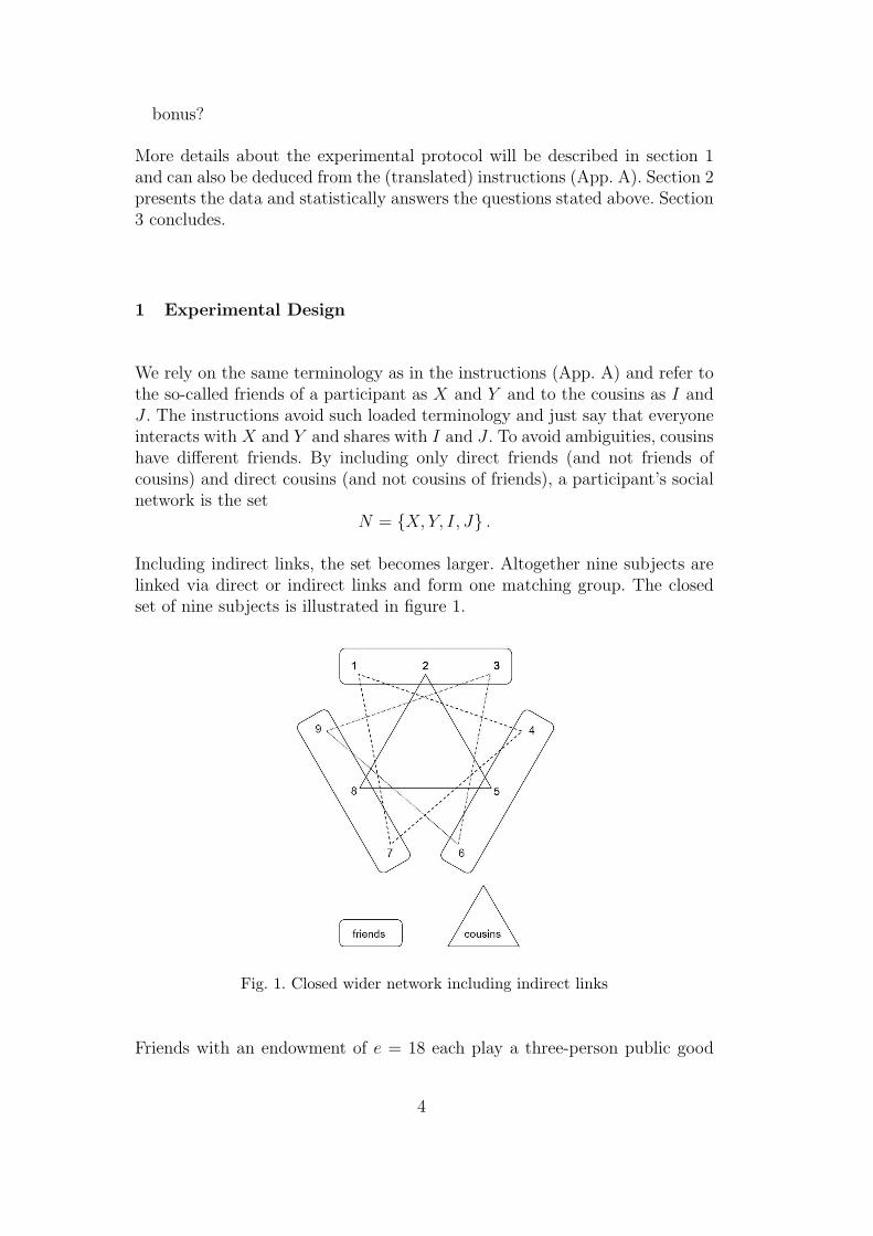
N = {X,Y, I, J} .

Including indirect links, the set becomes larger. Altogether nine subjects arelinked via direct or indirect links and form one matching group. The closedset of nine subjects is illustrated in figure 1.

Fig. 1. Closed wider network including indirect links

Friends with an endowment of e = 18 each play a three-person public good

4

game with a marginal per capita return of 2/3 and one’s own payoff

Po = 18 − o +2

3C with C = o + x + y and 0 ≤ o, x, y ≤ e

where o is the own and x or, resp., y, the contribution of X or, resp., Y . Thepayoff of a participant’s friends X and Y is analogously defined. Similarly,cousins I and J earn Pi and Pj in their separate public good games. Cousinsshare payoffs so that each of the three cousins earn half of the own payoff Po

and a quarter share of what each cousin has achieved. Thus a participant’sown total payoff is

Uo =1

2Po +

1

4Pi +

1

4Pj

which, of course, applies also to a participant’s cousins. Each participant is afriend or a cousin of two (different) other participants.

In more detail, the 1st phase of an experimental session started by readingthe instructions for the situation just described, and answering a few controlquestions. Then participants played the game just once and shared the rewardsas specified. A participant learned afterwards about

• the contribution vector in the own as well as in the two cousins’ games andthereby

• the payoffs in these three games.

The 2nd phase starts by informing each participant that half of the partici-pants will finally receive a job offer and that each job offer goes along withanother vacancy in the same firm for which they can recommend anybody oftheir social network. Thus, in principle, it is possible that each participantfinds a job. Actually, our assignment of job offers will guarantee that anybodywho has not received a direct job offer has at least one friend and one cousinwho could recommend him for the additional job opening. All job offers specify

• a fixed payment S = 4• a piece rate of s = 2• a bonus B = 18 attributable to the worker with the higher output (if both

produce the same output each gets B/2 = 9).

If a participant does not receive or accept a job, he is paid the unemploymentbenefit U = 12. If employed and producing a units, earnings are

S + δB + 2a − C(a) = 4 + δ18 + 2a −a2

8

where a2

8are the effort costs C(a) and, where δ equals 1 if an employee works

alone or, if not, has chosen the higher effort level, equals 1/2 when both producethe same, and is zero otherwise. The entire second stage is implemented using

5

a modified strategy vector method. Specifically, subjects first state whetherand, if so, whom they would recommend for the second vacancy before statingwhether they would accept such a direct or indirect offer themselves. 3 Whenstating whom they would recommend, subjects basically submit a ranking.In detail, subjects are asked sequentially up to four times whether they wantto recommend someone (else) and, if so, whom. Finally subjects submit theiroutput choices, if applicable for the four cases of working alone or with someoneelse and being directly or indirectly employed. This allows us to test whethercompeting for bonus B with a friend or cousin triggers greater efforts. In orderto avoid substantial losses, maximal effort was bounded from above.

We are, of course, especially interested in how recommendations depend on

• the type of relationship (are friends or cousins primarily recommended?)and

• the contributions (of friends) and the payoffs (of cousins), and how the latterare determined.

In more detail, phase 2 of the experiment started by reading the second partof the instructions 4 which were only distributed after the first phase, andanswering new control questions. Then all participants chose,

• in the case of a direct job offer, whether to accept it, and their recommen-dation policy as explained above

• in the case of receiving and accepting a direct and/or indirect job offer andselect their (up to four) effort choices.

After collecting all choices, jobs were directly assigned to half of the partici-pants. Their recommendations regarding the additional job offerings were im-plemented as were the effort choices of those who were thereby (co)employed.The experiment concluded by informing participants about the outcome con-cerning themselves and their direct network. Payments were made privatelyas to preserve anonymity.

The strategic analysis of the experimental game is straightforward. In the sec-ond stage, the rules of the labor market are independent of the entire firststage. When playing the first stage, subjects are not informed about the sec-ond. But even if they were informed about both stages, the outcome of first-stage interaction would not affect the rules of the labor market. The optimaleffort if working alone is e∗ = 8 yielding a payoff of 30. If coemployed, eachemployee has an incentive to outperform the other by one unit in order tosecure the bonus. Due to the quadratic cost function the resulting tournament

3 Thus, one can refuse a direct offer but nevertheless recommend someone for thesecond position in the firm.4 For a translation, see App. A.

6

for the bonus can be very destructive. We have restricted efforts to a max-imum of 17, implying that there exists no pure strategy equilibrium of thelabor market (sub)game(s). 5 Efficiency would require both to produce e∗ = 8and sharing the bonus, yielding 21 for each. Unless the second employee re-sorts to a dominated effort below 7, working alone yields a higher payoff thanbeing coemployed. Thus, the equilibrium play of the labor market is to accepta direct job offer, recommend nobody and produce a = 8 units as the onlyemployee.

2 Results

Nine sessions with 18 subjects each were conducted at the Computer Labora-tory of the Max Planck Institute of Economics in Jena in visually separatedPC Cabins. The experiment relied on the Z-tree software (Fischbacher, 1999),and subjects were students recruited from the Friedrich Schiller UniversitatJena, using the recruitment software ORSEE (Greiner, 2004) which guaran-teed that no subject participated more than once.

Including payment, sessions lasted for about 70 minutes. The exchange ratewas set to e1 for 5 points, amounting to a total endowment in the public goodgame of e3.60 and a maximum possible income from employment of e6. Noshow-up fee was paid. On average, subjects earned e9.26 (standard deviation1.94) with a minimum earning of e5.40, a median of e8.94, and a maximumof e13.36.

contribution ci

rel.

frequ

ency

0 5 10 15

0.00

0.05

0.10

0.15

0.20

0.25

0.30

PSfrag replacements

ci

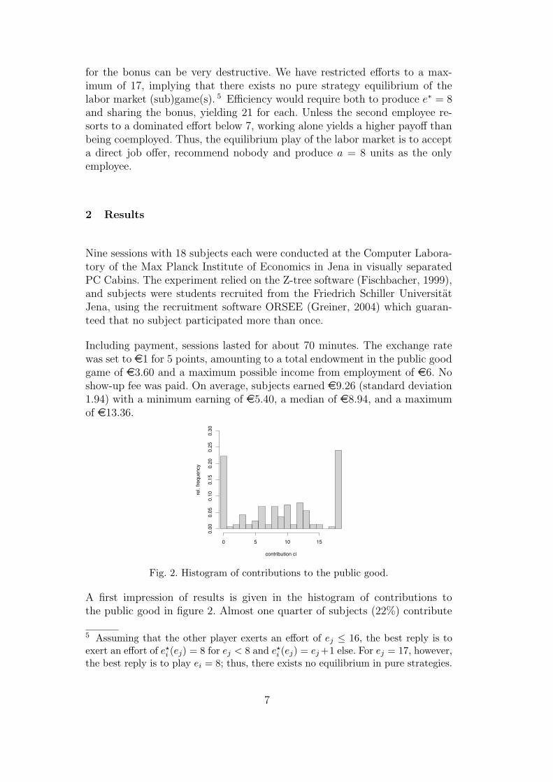
Fig. 2. Histogram of contributions to the public good.

A first impression of results is given in the histogram of contributions tothe public good in figure 2. Almost one quarter of subjects (22%) contribute

5 Assuming that the other player exerts an effort of ej ≤ 16, the best reply is toexert an effort of e?

i (ej) = 8 for ej < 8 and e?i (ej) = ej +1 else. For ej = 17, however,

the best reply is to play ei = 8; thus, there exists no equilibrium in pure strategies.

7

nothing and another quarter (24%) give their entire endowment. The averageand median contribution is 9 (standard deviation 6.68).

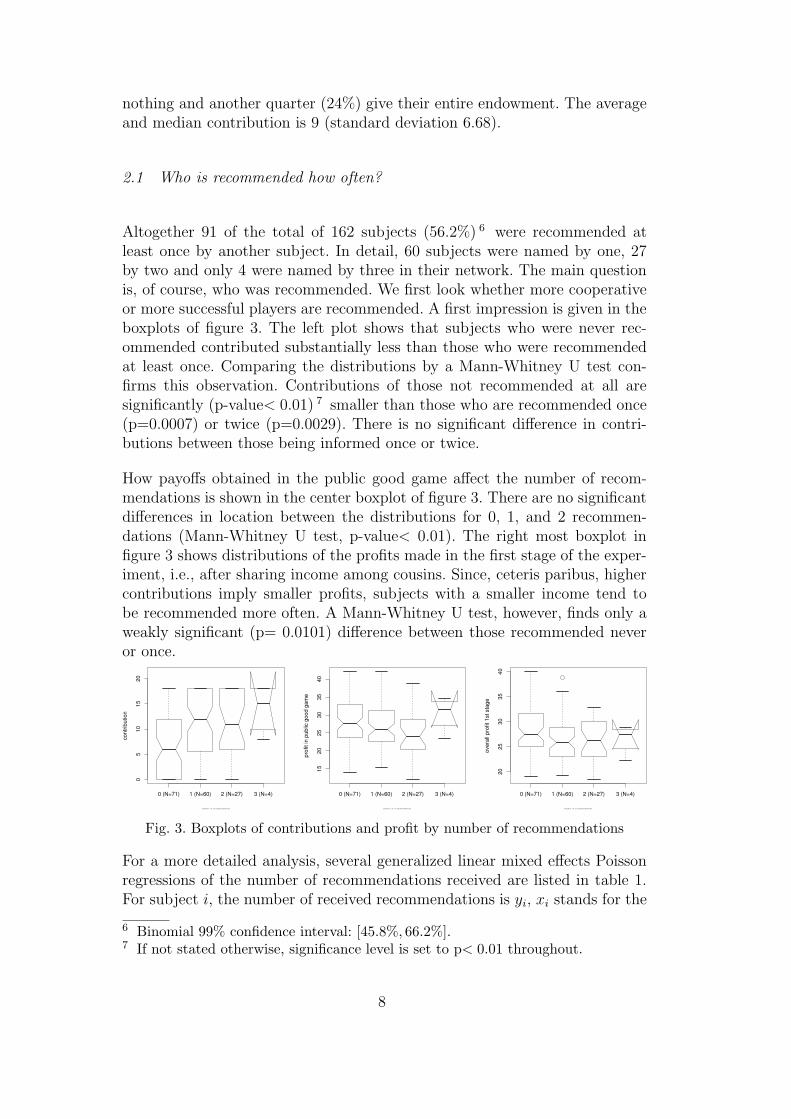
2.1 Who is recommended how often?

Altogether 91 of the total of 162 subjects (56.2%) 6 were recommended atleast once by another subject. In detail, 60 subjects were named by one, 27by two and only 4 were named by three in their network. The main questionis, of course, who was recommended. We first look whether more cooperativeor more successful players are recommended. A first impression is given in theboxplots of figure 3. The left plot shows that subjects who were never rec-ommended contributed substantially less than those who were recommendedat least once. Comparing the distributions by a Mann-Whitney U test con-firms this observation. Contributions of those not recommended at all aresignificantly (p-value< 0.01) 7 smaller than those who are recommended once(p=0.0007) or twice (p=0.0029). There is no significant difference in contri-butions between those being informed once or twice.

How payoffs obtained in the public good game affect the number of recom-mendations is shown in the center boxplot of figure 3. There are no significantdifferences in location between the distributions for 0, 1, and 2 recommen-dations (Mann-Whitney U test, p-value< 0.01). The right most boxplot infigure 3 shows distributions of the profits made in the first stage of the exper-iment, i.e., after sharing income among cousins. Since, ceteris paribus, highercontributions imply smaller profits, subjects with a smaller income tend tobe recommended more often. A Mann-Whitney U test, however, finds only aweakly significant (p= 0.0101) difference between those recommended neveror once.

0 (N=71) 1 (N=60) 2 (N=27) 3 (N=4)

05

1015

20

cont

ribut

ion

PSfrag replacementsnumber of recommendations

0 (N=71) 1 (N=60) 2 (N=27) 3 (N=4)

1520

2530

3540

prof

it in

pub

lic g

ood

gam

e

PSfrag replacementsnumber of recommendations

0 (N=71) 1 (N=60) 2 (N=27) 3 (N=4)

2025

3035

40

over

all p

rofit

1st

sta

ge

PSfrag replacementsnumber of recommendations

Fig. 3. Boxplots of contributions and profit by number of recommendations

For a more detailed analysis, several generalized linear mixed effects Poissonregressions of the number of recommendations received are listed in table 1.For subject i, the number of received recommendations is yi, xi stands for the

6 Binomial 99% confidence interval: [45.8%, 66.2%].7 If not stated otherwise, significance level is set to p< 0.01 throughout.

8

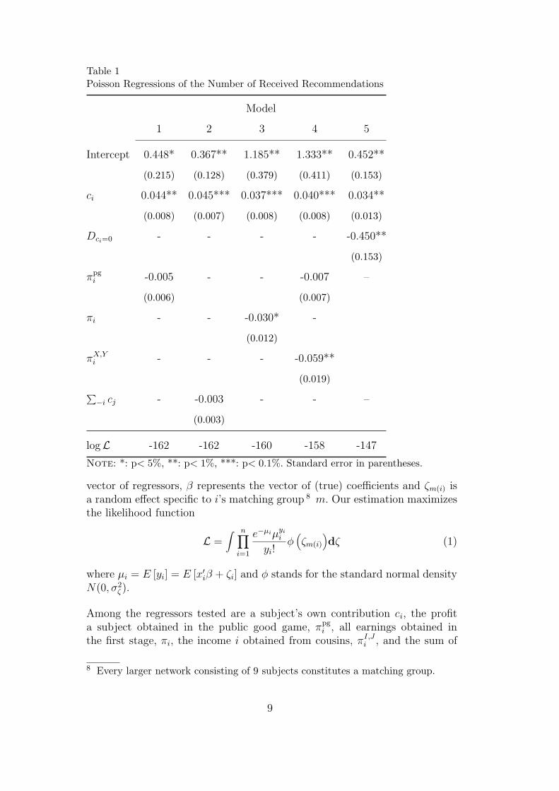
Table 1Poisson Regressions of the Number of Received Recommendations

Model

1 2 3 4 5

Intercept 0.448* 0.367** 1.185** 1.333** 0.452**

(0.215) (0.128) (0.379) (0.411) (0.153)

ci 0.044** 0.045*** 0.037*** 0.040*** 0.034**

(0.008) (0.007) (0.008) (0.008) (0.013)

Dci=0 - - - - -0.450**

(0.153)

πpgi -0.005 - - -0.007 –

(0.006) (0.007)

πi - - -0.030* -

(0.012)

πX,Yi - - - -0.059**

(0.019)

∑

−i cj - -0.003 - - –

(0.003)

logL -162 -162 -160 -158 -147

Note: *: p< 5%, **: p< 1%, ***: p< 0.1%. Standard error in parentheses.

vector of regressors, β represents the vector of (true) coefficients and ζm(i) isa random effect specific to i’s matching group 8 m. Our estimation maximizesthe likelihood function

L =∫ n

∏

i=1

e−µiµyi

i

yi!φ(

ζm(i)

)

dζ (1)

where µi = E [yi] = E [x′

iβ + ζi] and φ stands for the standard normal densityN(0, σ2

ζ ).

Among the regressors tested are a subject’s own contribution ci, the profita subject obtained in the public good game, πpg

i , all earnings obtained inthe first stage, πi, the income i obtained from cousins, πI,J

i , and the sum of

8 Every larger network consisting of 9 subjects constitutes a matching group.

9

contributions by friends,∑

−i cj.

Regression model 1 confirms that a subject is recommended more often themore he contributed to the public good. Due to the strong correlation betweenthe two regressors ci and πpg

i , model 2 substitutes profit by total contributionsby friends (

∑

−i cj) which is strongly correlated to the public good profit butnot to the own contribution. Model 2 validates the results from model 1.

Regression 3 finds only a weakly significant effect of the overall profit. Model4 qualifies this result by showing that the number of recommendations arenegatively correlated with the profit obtained from a subject’s cousins (πX,Y

i ).Model 5 explains our data best according to the Akaike and Schwartz informa-tion criteria. Here dummy Dci=0 indicates that the subject did not contribute.The coefficients of model 5 indicate that the number of recommendations is in-creasing with contributions and that free riders are heavily punished by beingrecommended significantly less often. A similar dummy, indicating full contri-bution (Dci=18), was tested but proved to be insignificant and not contributingto the accuracy of the model; there is thus no special acknowledgement of fullcontributions.

We summarize our first results by the following two observations:Observation 1 The best predictor for the number of received recommen-dations is a subject’s contribution to the public good. While the number ofrecommendations is increasing with a subject’s contribution, those contribut-ing nothing are additionally punished compared to those contributing at leastsomething.Observation 2 The profit a subject obtains in the public good stage has nodirect effect on the number of recommendations he is given. However, thereis some indication that subjects obtaining less (more) from their cousins aremore (less) often recommended.

2.2 Who recommends whom

A different way of approaching the data is by analyzing it from the perspectiveof the recommender. A subject could recommend each of his two friends andcousins. In the following, we therefore define the dependent variable as follows:the bivariate dependent yij stands for subject i ’s decision to recommend j.This interpretation of the data allows to test whether not only characteristicsof the recommendee but also characteristics of the recommender matter. Witha bivariate dependent, the model of choice is a generalized linear binomialmodel with a probit link.

To control for correlations within the four observations of each subject andwithin matching groups, we have added (nested) random effects. We define

10

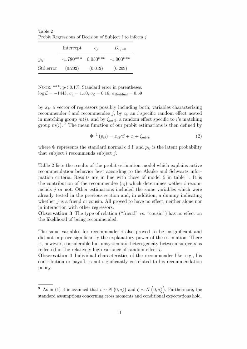
Table 2Probit Regressions of Decision of Subject i to inform j

Intercept cj Dcj=0

yij -1.780*** 0.053*** -1.003***

Std.error (0.202) (0.012) (0.209)

Note: ***: p< 0.1%. Standard error in parentheses.

logL = −1443, σς = 1.50, σζ = 0.16, σResidual = 0.59

by xij a vector of regressors possibly including both, variables characterizingrecommender i and recommendee j, by ςi, an i specific random effect nestedin matching group m(i), and by ζm(i), a random effect specific to i’s matchinggroup m(i). 9 The mean function of our probit estimations is then defined by

Φ−1 (pij) = xij′β + ςi + ζm(i), (2)

where Φ represents the standard normal c.d.f. and pij is the latent probabilitythat subject i recommends subject j.

Table 2 lists the results of the probit estimation model which explains activerecommendation behavior best according to the Akaike and Schwartz infor-mation criteria. Results are in line with those of model 5 in table 1. It isthe contribution of the recommendee (cj) which determines wether i recom-mends j or not. Other estimations included the same variables which werealready tested in the previous section and, in addition, a dummy indicatingwhether j is a friend or cousin. All proved to have no effect, neither alone norin interaction with other regressors.Observation 3 The type of relation (“friend” vs. “cousin”) has no effect onthe likelihood of being recommended.

The same variables for recommender i also proved to be insignificant anddid not improve significantly the explanatory power of the estimation. Thereis, however, considerable but unsystematic heterogeneity between subjects asreflected in the relatively high variance of random effect ς.Observation 4 Individual characteristics of the recommender like, e.g., hiscontribution or payoff, is not significantly correlated to his recommendationpolicy.

9 As in (1) it is assumed that ς ∼ N(

0, σ2ς

)

and ζ ∼ N(

0, σ2ζ

)

. Furthermore, the

standard assumptions concerning cross moments and conditional expectations hold.

11

2.3 Accepting offers and working effort

After deciding whether and whom to recommend subjects had to state whetherthey would accept a direct and/or indirect offer. Except for two subjects ev-eryone (160) would have accepted a direct offer, and altogether 149 (92%)would have accepted an indirect offer. Given the small number of rejections,no meaningful inferences can be made concerning differences between thoseaccepting and rejecting an offer. Interestingly, the 13 subjects who rejected anindirect offer on average contributed more (10 vs. 8.98) and earned less in thepublic good game (23.4 vs. 27.4) and overall in the first stage (24.5 vs. 27.3).

The number of effort levels a subject has to submit depends on whether or nothe would recommend one of his network and whether he accepts a(n) (in)directoffer. Those who recommended at least one and would have accepted any offerwere, for instance, asked four times to submit an effort choice: in case of adirect as well as an indirect offer and working alone, and in case of a direct aswell as an indirect offer but being coemployed. On the other hand, a subjectwho rejected every job offer did not submit any effort level.

The marginal effects of obtaining a direct vs. an indirect offer and of workingalone vs. being coemployed on the effort level are plotted in figure 4. The firstboxplot plots the differences in efforts between being directly and indirectlyemployed. The third and fourth boxplots basically plot the same differencesthough separately for efforts by the employee working alone (third plot) orwhen being coemployed (fourth plot). All boxplots use data of only thosesubjects with observations for all relevant cases. The first boxplot, e.g., requiresdata for all four possible encounters, which was the case for 59 subjects.

As observations within one matching group are likely to be correlated, aver-ages over matching groups are used to obtain independent data. 10 Accordingto the first boxplot, efforts do not depend on whether one is employed di-rectly or indirectly (Wilcoxon signed rank test, p=0.103). Comparing effortsregarding working alone or being coemployed in the second boxplot, revealsa strong competition effect. When working alone, 24 of the 59 subjects withfour effort choices play optimally (effort of 8). When being coemployed, mostincrease their effort and only seven maintain the optimal effort. Overall, whenworking alone efforts are significantly smaller than in case of being coemployed(Wilcoxon signed rank test, p<0.1%).Observation 5 When coemployed, subjects make significantly greater effortsthan when working alone.

10 While producing pairwise independent observations, this method is not unprob-lematic as the number of observations per matching group may differ. For thatpurpose, all tests reported were also conducted with individual level data, ignoringpossible dependencies. Qualitative results are identical.

12

−8−6

−4−2

02

PSfrag replacements

diff

ere

nce

ineffort

s

.direct–

indirect(N = 59)

.alone–two

(N = 59)

ALONE:

direct–

indirect(N = 148)

TWO:

direct–

indirect(N = 59)

DIRECT:

alone–two

(N = 61)

INDIRECT:

alone–two

(N = 149)

Note: Differences of averages per matching group. N is number ofsubjects for whom observations are available in both conditions.

Fig. 4. Boxplots of Differences in Efforts

This result is partly confirmed by the remaining boxplots. Only for an em-ployee working alone are efforts significantly (Wilcoxon signed rank test, p=0.007)greater in case one was hired directly. With an average of 0.5, this differenceis, however, rather negligible.

The strong evidence of a (destructive) competition for the bonus in case ofcoemployment raises an important question: Are more cooperative playersof the public good game recommended in the hope that they refrain fromcompeting for the bonus? The fourth boxplot in figure 4 gives a first answer tothis question: Under coemployment, efforts of those directly employed do notdiffer significantly from efforts of those indirectly employed. Thus, subjects donot care about the source of their employment when competing for the bonus.But is there at least a negative correlation between the own effort and thecontribution of the recommended coworker?

Table 3 lists several tobit regressions of effort choices for being directly em-ployed and competing for the bonus with someone the subject has himselfrecommended. Ignoring the intercept, the first three variables are character-istics of the decider: ealone

d,i is the effort of the decider when being directlyemployed but working alone, ci his own contribution to the public good, andratioi a dummy with 1 for ealone

d,i = 8. The last four variables concern the onerecommended: cj,1 is the contribution to the public good of the one recom-mended first, Dfriend

j1 a dummy with value 1 when this first recommendationrefers to a friend, cj,1D

friendj1 the interaction between the two variables, and cj

the average contributions by all recommended by i. According to model 1 and2, the effort choice is completely independent of what happened previously.

13

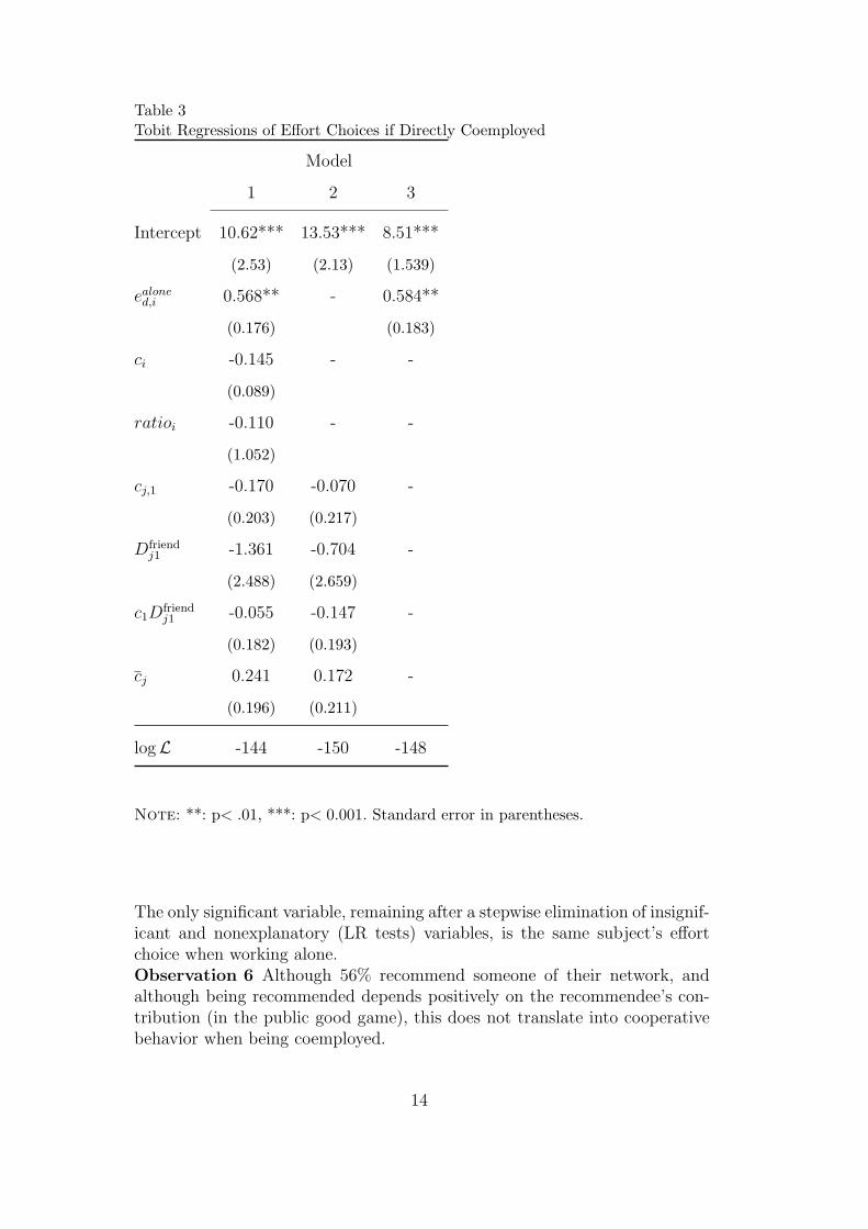
Table 3Tobit Regressions of Effort Choices if Directly Coemployed

Model

1 2 3

Intercept 10.62*** 13.53*** 8.51***

(2.53) (2.13) (1.539)

ealoned,i 0.568** - 0.584**

(0.176) (0.183)

ci -0.145 - -

(0.089)

ratioi -0.110 - -

(1.052)

cj,1 -0.170 -0.070 -

(0.203) (0.217)

Dfriendj1 -1.361 -0.704 -

(2.488) (2.659)

c1Dfriendj1 -0.055 -0.147 -

(0.182) (0.193)

cj 0.241 0.172 -

(0.196) (0.211)

logL -144 -150 -148

Note: **: p< .01, ***: p< 0.001. Standard error in parentheses.

The only significant variable, remaining after a stepwise elimination of insignif-icant and nonexplanatory (LR tests) variables, is the same subject’s effortchoice when working alone.Observation 6 Although 56% recommend someone of their network, andalthough being recommended depends positively on the recommendee’s con-tribution (in the public good game), this does not translate into cooperativebehavior when being coemployed.

14

3 Conclusions

To experimentally observe why and when friends or relations help someone tofind a job, we have created a stylized social network. We could explore whetherand how the type of relation (“friends” playing a public good game versus“cousins” with whom one shares the profit) and former behavior influencewho is recommended, and how likely it is to be recommended. To capture andmodel the possible competition when being coemployed, participants finallyhad to make effort choices.

Our results show that it is not the type of relation nor individual earnings(in the public good game) which affect the chances on the job market, butrather cooperativeness toward others, as measured by the contribution to thepublic good. We were thus able to identify an endogenous characteristic bywhich subjects discriminate among their network peers. Here it is importantto stress that this behavior cannot be explained merely by direct reciprocity,as not only “friends” but also “cousins” are equally rewarded for cooperativebehavior. Interestingly, despite creating an anchor for discrimination, behaviorin the first stage is ignored when competing for a bonus. While a subject ismore likely to recommend someone with higher contributions and is morelikely to be recommended when contributing more, this does not affect effortchoices when competing.

We conclude from this that our participants view filling job vacancies by some-one suitable, i.e., with a high contribution revealing cooperativeness, as amoral obligation. This, however, does not question that a participant competesvery seriously for promotion or a bonus when being coemployed. It remindsus of doing sports together where, for example, I might give someone a lift tothe racetrack but will nevertheless try to outrun him or her in the race. Thatsome of our choices, here job recommendations, are guided by ethical motivesand others by opportunism, is a familiar idea in welfare economics (see, e.g.,the distinction between individual welfare and individual utility functions byHarsanyi, 1977). Our findings show that this distinction may apply even whenfacing the same person.

Related to the job market, we seem to justify using social networks for recruit-ment in a worst-case scenario of rather weak links (but also of rather minoreffects). We seem to recommend someone suitable, even when afraid of suf-fering from that later on. Concern that a workforce consisting of friends andrelatives may be burdened by sluggishness and inefficiency is not confirmedby our data.

We do not claim that our conclusions are generally transferable to the realworld. While the lack of carry-over effects from the first to the last stage is

15

one main observation, it may also question the effectiveness of inducing asocial network experimentally and of distinguishing “friends” and “relatives”.Of course, we could have relied on voluntary network formation games. 11

Compared to our approach, a network first has to be established endogenously,rendering such voluntary network formation experiments rather intractablewhen being followed by a job market.

References

Blau, D. M., Robins, P. K., june 1990. Job search outcomes for the employedand unemployed. The Journal of Political Economy 98 (3), 637–655.

Calvo-Armengol, A., Jackson, M. O., jun 2004. The effects of social networkson employment and inequality. American Economic Review 94 (3), 426–454.

Corcoran, M., Datcher, L., Duncan, G., 1980. Most workers find jobs throughword of mouth. Monthly Labor Review 103, 33–35.

Falk, A., Fischbacher, U., Gachter, S., 2004. Living in two neighborhoods:Social interactions in the lab. IZA Discussion Paper 1381.

Fischbacher, U., 1999. Z-tree: A toolbox for readymade economic experiments.Working Paper No. 21, Institute for Empirical Research in Economics –University of Zurich.

Granovetter, M. S., 1974. Getting a job: a study of contacts and careers. TheUniversity of Chicago Press, Chicago.

Greiner, B., 2004. An online recruitment system for economic experiments. In:Kremer, K., Macho, V. (Eds.), Forschung und wissenschaftliches Rechnen2003. Gesellschaft fur Wissenschaftliche Datenverarbeitung, Gottingen, pp.79–93, gWDG Bericht 63.

Guth, W., Levati, M. V., Ploner, M., 2005. On the social dimension of timeand risk preferences: An experimental study. Discussion Papers on StrategicInteraction 26-2005.

Harsanyi, J. C., 1977. Rational Behavior and Bargaining Equilibrium in Gamesand Social Situations. Cambridge University Press, Cambridge, Mass.

Holzer, H. J., jan 1988. Search method use by unemployed youth. Journal ofLabor Economics 6 (1), 1–20.

Noll, H.-H., Weick, S., jul 2002. Informelle kontakte fur zugang zu jobswichtiger als arbeitsvermittlung. Informationsdienst Soziale Indikatoren(ISI) 28, 6–11.

Roth, A. E., jan 1984. Stability and polarization of interests in job matching.Econometrica 52 (1), 47–57.

Tajfel, H., 1970. Experiments in intergroup discrimination. Scientific American223, 96–102.

The Economist, 2006. Squaring the circle. Print Edition, February 11th, 2006.

11 See, e.g., Calvo-Armengol and Jackson (2004) for an analysis of voluntary net-works and their effects on the job market.

16

A Translation of Instructions and Control Questions

The following subsections give a translation into English of the German in-structions and control questions. Emphasizes are as in the original.

A.1 Instructions for the Public Good Game

General Instructions

Welcome and thank you for participating in this experiment. Depending onyour decisions and the decisions of other participants, you will earn money.Therefore it is of the utmost importance that you read these instructionscarefully.

During the experiment any kind of communication with other participantsis categorically forbidden. In case you have questions, please raise your armand ask one of the supervisors. If you break this rule, we will have to excludeyou from the experiment and you will not receive any money. Instructions areidentical for all participants.

During the experiment monetary amounts are not denoted in ebut in “points”.At the end of the experiment, your total points are converted to eaccordingto the following exchange rate:

5 points = 1 e

Now please read the following instructions carefully.

Detailed Instructions

The Decision Environment

You will interact with two interaction partners, X and Y . Furthermore, youwill share your interaction income with two other participants, I and J . Thesame holds for all other participants in the experiment. However, I and Jneither interact with each other nor with participant X or Y , with whom youinteract.

Thus, you (denoted as O in the following) are a member of the group of 3

O, X, Y . Each member of this group has to decide how to use 18 points. Youcan assign your 18 points to your private account or you can invest some

or all of them in a project. Every point not invested into the project willautomatically be assigned to your private account.

17

Income from the private account:

For every point you leave on your private account you will earn exactly onepoint. If, for example, you leave 18 points on your private account (and there-fore do not invest anything into the project), you will earn exactly 18 pointsfrom your private account. Or, if you leave exactly 1 point on your privateaccount, you will receive exactly 1 point from your private account. No oneexcept you earns something from your private account.

Income from the project:

From the amount you invest into the project, every group member earns anequal share. Conversely it holds that you profit from the investment of theother group members. The income of each member from the project is definedas follows:

Income from the project = Sum of all investments into the project times 2/3

If, for example, the sum of investments into the project of all group membersequals 30 points, then you and every other group member each earn 30× 2/3 =20 points from the project. If the three group members invest altogether 1point into the project, then you and each other group member each earn1 × 2/3 = 0.67 points from the project.

Interaction income:

Your interaction income Po is the sum from your income of the private accountand from the project. Thus:

Income from your private account (= 18 - contribution to theproject)

+ Income from the project (= 2/3× sum of contributions to the project)= interaction income

In different notation: Po = 18 − o + C × 2/3 where C = o + x + y equals thesum of your contribution o plus contributions x from X and y from Y .

Total income after sharing:

Similarly, participants I and J assigned to you earned, together with theirinteraction partners, their interaction income Pi and Pj. From your interactionincome Po, participants I and J now receive one quarter each. Equivalently,you receive one quarter of each of I and J ’s interaction income. Your totalincome is thus defined as follows:

18

You keep half of your interaction income+1/4 interaction income of I+1/4 interaction income of J

= total income

That is, you obtain Po/2 + Pi/4 + Pj/4. Equivalently, participant I earns Pi/2 +Po/4 + Pj/4 and J earns Pj/2 + Pi/4 + Po/4.

You can make this decision only once. There will be no repetition.

A.2 Control Question for the Public Good Game

Control Questions

Please answer the following questions. They are designed to acquaint you withthe calculation of incomes. The examples are chosen such that you can easilysolve them without a calculator.

Please answer all questions, always noting the entire formula.

1. Each participant of group O,X, Y has 18 points at his disposal. Assumethat all thre group members (including O) invest nothing into the project.How much is your interaction income?How much is the interaction income of each of the other group members?

2. Each participant of group O,X, Y has 18 points at his disposal. You invest18 points into the project. The other group members also invest 18 pointseach. How much is your interaction income?How much is the interaction income of each of the other group members?

3. Each participant of group O,X, Y has 18 points at his disposal. The othertwo group members together invest 18 points into the project.

a) How much is your interaction income if you, in addition to the 18 points,invest nothing into the project? Your interaction income:

b) How much is your interaction income if you, in addition to the 18 points,invest 9 points into the project? Your interaction income:

b) How much is your interaction income if you, in addition to the 18 points,invest 18 points into the project? Your interaction income:

4. Each participant of group O,X, Y has 18 points at his disposal. You invest12 points into the project.

a) How much is your interaction income if the other group members – inaddition to your 12 points – together invest 9 points into the project?Your interaction income:

19

b) How much is your interaction income if the other group members – inaddition to your 12 points – together invest 21 points into the project?Your interaction income:

c) How much is your interaction income if the other group members – inaddition to your 12 points – together invest 36 points into the project?Your interaction income:

5. What share of your interaction income do you keep for yourself?6. What share of your interaction income does I receive?7. What share of J ’s interaction income do you receive?8. What share of your interaction income does participant K receive, who

directly interacted with J and obtained interaction income PK?9. Assume your interaction income is 12, that of I is 40, and that of J is 24.

a) How much is your total income?a) How much is the total income of J?

A.3 Instructions Labor Market

Instructions 2nd Part

Situation

You as well as participants X, Y , I, and J assigned to you in the first partof the experiment are workers. In total, there are twice as many workers asemployers. 12 Each employer has two vacancies. However, all employers firstdemand only one employee. One half of all participants therefore gets a directjob offer. You are free to decide whether to accept a job offer or not. Togetherwith the direct offer, participants obtain the information that there is a secondvacancy with that employer. Independently of whether they accept the directjob offer, these participants can recommend one or several of participants X,Y , I, and J for that second position. A participant who was recommendedcan in turn accept or reject that position.

A job offer consists of a fixed wage S = 4, a piece wage of 2a, where a is thequantity produced by the employee, and a bonus B = 18. Quantity a mustat least be 0 and cannot be greater than 17.

You will only obtain the bonus either if you are the only employee or, if not,if your quantity is larger than that of your colleague. If both of you producethe same quantity, each employee obtains half of the bonus, i.e., B/2 = 9.

Furthermore, working is costly for the employee. These costs are dependent on

12 In the experiment the employers are atomized and not represented by partici-pants.

20

quantity a and equal a2/b. Thus, your payoff of being employed and producinga equals:

fixed wage S = 4+ if you work alone or, if not, if your quantityis larger than your colleague’s: Bonus B = 18

or, if quantities are identical: B/2 = 9+ piece wage: 2a

- costs of working: a2/8

= labor income

If you remain without a job, you receive a payment of U = 12.

Implementation

Direct Offer

At first you will not be informed about whether you received a direct job offer.Initially, you will decide in case you received a direct job offer if and, if so,who of X, Y , I and J you recommend for the second vacancy. Thereby, youcan make up to four statements. That is you submit a ranking which specifieswho you would recommend in which order. 13

Subsequently, you indicate whether you want to accept a direct offer. If youdo so, you are asked for your quantity a. If you recommended at least oneparticipant for the second vacancy, you are asked to make two statementsconcerning a: One in case you remain alone – i.e., the second vacancy remainsvacant – and one in case you are one of two employees.

No Direct Offer but Recommended for Second Position

After deciding in the case of receiving a direct offer, you are asked to decidein the case of not receiving a direct offer but for being recommended for thesecond vacancy. Thereby, you first indicate, whether you accept this positionand if so, how much you produce, once in case you work alone (the participantwho obtained the direct offer rejected) and once in case you are one of twoemployees.

Calculation of Incomes

After making all your decisions a random draw decides who obtains a directoffer. Thereby it is guaranteed that at least one of participants X, Y , I, andJ , assigned to you, obtains a direct offer. Finally, your income and, if you havea colleague, that of your coworker are calculated and listed on your screen.

13 If several participants recommend the same participant, a random draw decides.

21

You can make your decisions only once. There will be no repetition.

A.4 Control Question for Labor Market

Control Questions 2nd Part

Please answer the following questions. They are designed to acquaint you withthe calculation of incomes. The examples are chosen such that you can easilysolve them without a calculator.

Please answer all questions, always noting the entire formula.

1. Assume you receive a direct offer:a) How much do you earn if you recommend someone for the second vacancy,

he then accepts, produces a = 11, but you yourself reject the direct joboffer?

b) How much do you earn if you accept the direct job offer, do not recommendsomeone and produce a = 4?

c) How much do you earn if you accept the direct job offer, recommendsomeone for the second position, he rejects, and you yourself producea = 16?

d) How much do you earn if you accept the direct job offer, recommendsomeone for the second position, he accepts, you yourself produce a = 4,and the other produces a = 16?

e) How much do you earn if you accept the direct job offer, recommendsomeone for the second position, he accepts, you yourself produce a = 4,and the former produces a = 4?

2. Assume you receive no direct job offer:a) How much do you earn if you are not recommended for the second va-

cancy?b) How much do you earn if you are recommended for the second vacancy

but reject?c) How much do you earn if you are recommended for the second vacancy, ac-

cept, produce a = 16 but work alone as the participant who recommendedyou rejected the direct job offer?

d) How much do you earn if you are recommended for the second vacancy,accept, are coemployed, produce a = 16 yourself and your colleague pro-duces a = 4?

e) How much do you earn if you are recommended for the second vacancy, ac-cept, are coemployed, produce a = 4 yourself and your colleague producesa = 4?

f) How much do you earn if you are recommended for the second vacancy, ac-cept, are coemployed, produce a = 4 yourself and your colleague produces

22

a = 17?

23