Embed Size (px)
Citation preview
-A193 970 DEVELOPMENT AND EVALUATION OF A MONTE CARLO CODE SYSTEM I.FOR ANALYSIS OF IONIZATION CHAMBER RESPONSES(U) OAKRIM NATIONAL LAI TN J 0 JOHNRON ET AL. JUL 67
UNCLASSIFI ED ORN/TN-1 l / FI 1/4NL
omhmhmmmls
so/momoaamosoIIIIIIIIIIIIIIIIIIIIIIIIIIII
UlmlAMA
' viANMg O" IOrKN TEST C NM
%II
LI- " '"' 'B \ e."au" - 'q p --~ %%'m
OAK RIDGENATIONALLABORATORY Development and Evaluation of
a Monte Carlo Code System-c for Analysis of Ionization
C Chamber Responses
(V~ J. 0. JohnsonT. A. Gabriel
DTIO0 S ELECTE
AUG62 OW
D
DO-MMMUTONSTP.TE4mEN-Approved for public xeleaseq
-Distuibution Ulimitcd
IU1 ETTfA MWn SYSTES. 0C.
NOW a MIR 8 14 003
Printed in the United States of America. Available fromNational Technical Information Service
U.S. Department of Commerce5285 Port Royal Road. Springfield, Virginia 22161
NTIS price codes-Printed Copy: A06 Microfiche A01
This report was prepared as an account of work sponsored by an agency of theUnited States Government. Neither theUnited States Government nor any agencythereof, nor any of their employees, makes any warranty, express or implied, orassumes any legal liability or responsibility for the accuracy, completeness, oruaefulness of any information, apparatus, product, or process disclosed, orrepresents that its use would not inf ringeprivately owned rights. Reference hereinto any specific commercial product, process, or service by trade name, trademark.manufacturer, or otherwise, does not necessarily constitute or imply itsendorsement, recommendation, or favoring by the United States Government orany agency thereof. The views and opinions of authors expressed herein do notnecessarily state or reflect those of the United States Government or any agencythereof.
1 e
OEXNL/TM- 10196
Engineering Physics and Mathematics Division
DEVELOPMENT AND EVALUATION OF A MONTE CARLO CODE SYSTEM
FOR ANALYSIS OF IONIZATION CHAMBER RESPONSES
J. 0. JohnsonT. A. Gabriel
Accesioli For
Date Published: July 1987 NTIS CRA&I
UP annot., -cedT-* tfca lIon
BY
This Work Sponsored byDefense Nuclear Agency Ai3.hIyCodes
UnderInteragency Agreement No. 40-65-65 011 st A.,a.1
Prepared by theOAK RIDGE NATIONAL LABORATORY 0"Oak Ridge, Tennessee 37831
operated by 00NSMARTIN MARIETTA ENERGY SYSTEMS, INC.
for theU.S. DEPARTMENT OF ENERGY
under contract DE-AC05-840R21400
..... .
TABLE OF CONTENTS
CHAPTER PAGE
LIST OF TABLES. ......................... iv
LIST OFFIGURES ......................... vi
ACKNOWLEDGMENTS .. ........................ ix
ABSTRACT .............................. X
I. INTRODUCTION .. ................. . .. 1
1.0 Background .. ...................... 21.1 Need for the Present Work. ............... 51.2 Project Objectives .. .................. 61.3 Calculational Procedure. ................ 71.4 Originality of Present Work. .............. 8
II. APPLICATION OF MONTE CARLO TO THE SOLUTIONOF THE TRANSPORT EQUATION. .. ............... 11
2.0 Boltzmann Transport Equation. .. ........... 112.1 Random Walk Procedure .. ............... 19
III. NUCLEAR PROCESSES .. .................... 30
3.0 Introduction. .. .................... 303.1 Neutron Interactions. .. ............... 303.2 Photon Interactions .. ................ 373.3 Electron Interactions .. ............... 393.4 Charged Particle Interactions .. ........... 40
IV. SYSTEM VERIFICATION AND RESULTS. .. ............ 43
4.0 Introduction. .. ................... 434.1 Comparison with MORSE .. ............... 454.2 Comparison with MACK-IV and RECOI .. .. ....... 574.3 Comparison with 05S.. ................ 624.4 Comparison with Photon Calibration Experiments .. . 684.5 Comparison with Mixed Field Experiments. .. ..... 83
V. CONCLUSIONS .. ....................... 95
VI. RECOMMENDATIONS FOR FUTURE WORK. .. ............. 97
LIST OF REFERENCES. ....................... 99
LIST OF TABLES
TABLE PAGE
4-1. Material Parameters for the Iron Slab ... ...... .... 46
4-2. Comparison of MICAP and MORSE Integral Quantitiesfor the 50 cm x 50 cm x 10 cm Iron Slab with a PointMono-Directional Fission Neutron Source ........... ... 52
4-3. Comparison of MICAP and MORSE Integral Quantitiesfor the 50 cm x 50 cm x 10 cm Iron Slab with a PointMono-Directional 14.2 MeV Neutron Source .. ........ .. 52
4-4. Comparison of MICAP and MORSE Integral Quantitiesfor the 50 cm x 50 cm x 20 cm Iron Slab with a PointIsotropic Fission Neutron Source .... ............ .53
4-5. Comparison of MICAP and MORSE Integral Quantitiesfor the 50 cm x 50 cm x 20 cm Iron Slab with a PointIsotropic 14.0 MeV Neutron Source .... ............ .53
4-6. Comparison of MICAP and MORSE Integral Quantitiesfor the 50 cm x 50 cm x 20 cm Iron Slab with a PointIsotropic 14.0 MeV Neutron Source and using theENDF/B-IV and ENDF/B-V Cross Section Data Bases ....... 54
4-7. Comparison of PHOTON and MORSE Integral PhotonLeakage out the Back Face of the Iron Slab Usingthe MORSE Generated Secondary PhotonProduction Data ........ ..................... ... 56
4-8. Iron Microscopic Cross Sections (at 14.2 MeV)Used in the MICAP, MACK-IV, and RECOIL KermaFactor Calculations ....... ................... ... 59
4-9. Comparisonof MICAP and MACK-IV Average KineticEnergies (E) and Kerma Factors for the PartialReactions at 14.2 MeV ....... .................. .60
't-10. Comparisonof MICAP and RECOIL Average KineticEnergies (E) and Kerma Factors for the PartialReactions at 14.2 MeV ............... .. 61
'-11. Material Parameters for the BC501Polyvinyltoluene Plastic Scintillator ... .......... .63
4-12. Material Parameters for the Health andSafety Laboratory (HASL) High Pressure ArgonIonization Chamber ....... ................... . 69
iv
TABLE PAGE
4-13. Material Parameters for the Armed ForcesRadiobiology Research Institute (AFRRI)Ionization Chambers ....... ................... ... 72
4-14. Comparison of Measured and CalculatedDetector Responses for the Photon CalibrationExperiments of the Health and SafetyLaboratory (HASL) High PressureArgon Ionization Chamber ...... ................ .77
4-15. Comparison of Measured and CalculatedDetector Responses for the Photon CalibrationExperiments of the Armed Forces RadiobiologyResearch Institute (AFRRI) 50 cm
3
Ionization Chambers ....... ................... ... 79
4-16. Comparison of Measured and CalculatedDetector Responses for the Photon Calibration
Experiments of the Armed Forces RadiobiologyResearch Institute (AFRRI) 0.5 cm
3 and 0.05 cm3
Ionization Chambers ....... ................... ... 80
4-17. Primary Neutron Source Spectra Used in theArmed Forces Radiobiology Research Institute(AFRRI) Mixed Neutron and Photon RadiationField Ionization Chamber Calculations ... .......... .86
4-18. Primary Photon Source Spectra Used in the
Armed Forces Radiobiology Research Institute(AFRRI) Mixed Neutron and Photon RadiationField Ionization Chamber Calculations .......... 87
4-19. Comparison of Measured and CalculatedDetector Responses for the Mixed Neutron andPhoton Radiation Field Experiments of theArmed Forces Radiobiology Research Institute(AFRRI) Ionization Chambers ...... .............. .90
4-20. Comparison of Measured and CalculatedDetector Response Components for the MixedNeutron and Photon Radiation Field Experimentsof the Armed Forces Radiobiology ResearchInstitute (AFRRI) Ionization Chambers ... .......... .93
v
9 9 9 9e
LIST OF FIGURES
FIGURE PAGE
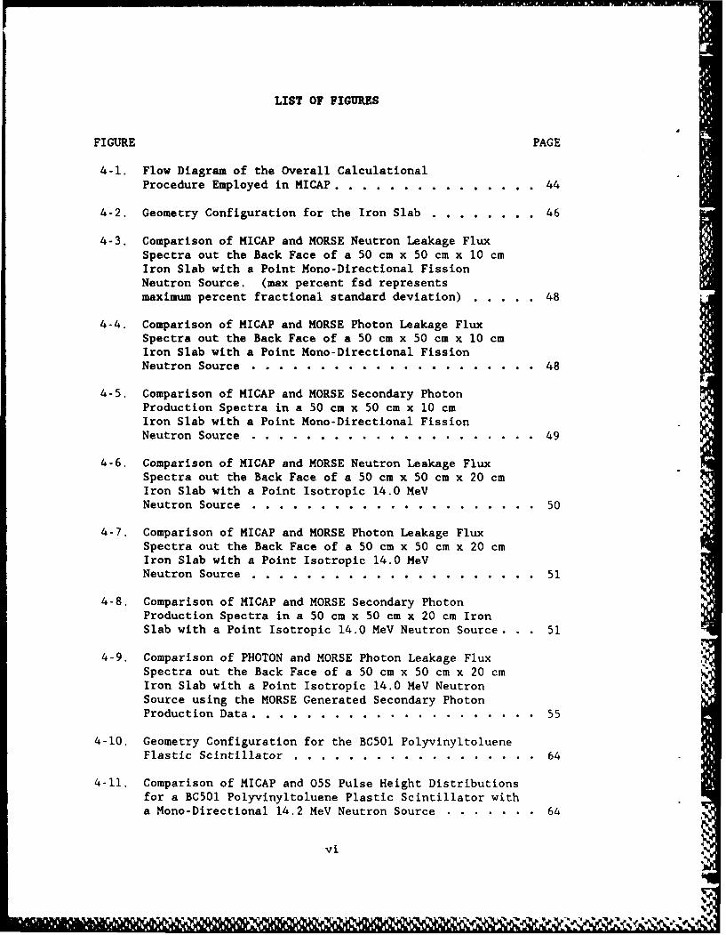
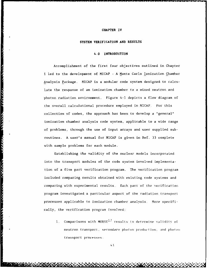
4-1. Flow Diagram of the Overall CalculationalProcedure Employed in MICAP ..... ............... ... 44
4-2. Geometry Configuration for the Iron Slab .. ....... ... 46
4-3. Comparison of MICAP and MORSE Neutron Leakage FluxSpectra out the Back Face of a 50 cm x 50 cm x 10 cmIron Slab with a Point Mono-Directional FissionNeutron Source. (max percent fsd representsmaximum percent fractional standard deviation) ..... ... 48
4-4. Comparison of MICAP and MORSE Photon Leakage FluxSpectra out the Back Face of a 50 cm x 50 cm x 10 cmIron Slab with a Point Mono-Directional FissionNeutron Source ........ ..................... . 48
4-5. Comparison of MICAP and MORSE Secondary PhotonProduction Spectra in a 50 cm x 50 cm x 10 cmIron Slab with a Point Mono-Directional FissionNeutron Source ......... .................... . 49
4-6. Comparison of MICAP and MORSE Neutron Leakage FluxSpectra out the Back Face of a 50 cm x 50 cm x 20 cmIron Slab with a Point Isotropic 14.0 MeVNeutron Source ........ ..................... . 50
4-7. Comparison of MICAP and MORSE Photon Leakage FluxSpectra out the Back Face of a 50 cm x 50 cm x 20 cmIron Slab with a Point Isotropic 14.0 MeVNeutron Source ........ ..................... . 51
4-8. Comparison of MICAP and MORSE Secondary PhotonProduction Spectra in a 50 cm x 50 cm x 20 cm IronSlab with a Point Isotropic 14.0 MeV Neutron Source. . . 51
4-9. Comparison of PHOTON and MORSE Photon Leakage FluxSpectra out the Back Face of a 50 cm x 50 cm x 20 cmIron Slab with a Point Isotropic 14.0 MeV NeutronSource using the MORSE Generated Secondary PhotonProduction Data ........ ..................... ... 55
4-10. Geometry Configuration for the BC501 PolyvinyltoluenePlastic Scintillator ....... .................. . 64
4-11. Comparison of MICAP and 05S Pulse Height Distributionsfor a BC501 Polyvinyltoluene Plastic Scintillator witha Mono-Directional 14.2 MeV Neutron Source ........ . 64
vi
d lat: I~ w tl4,O
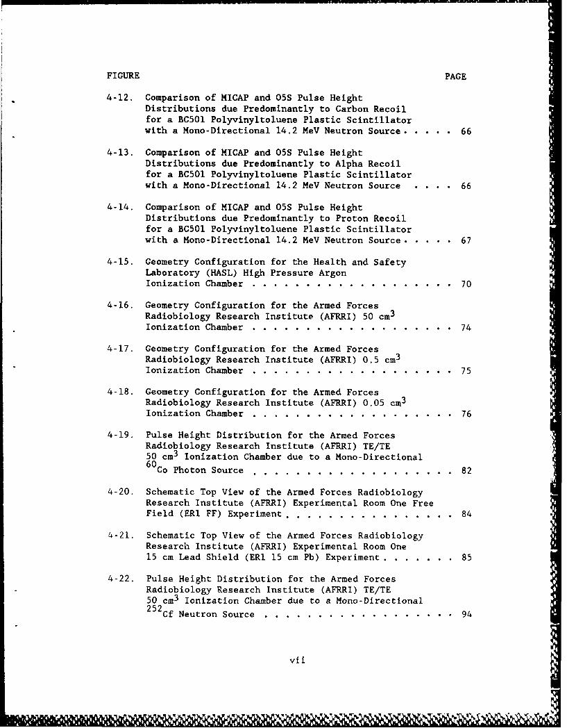
FIGURE PAGE
4-12. Comparison of MICAP and 05S Pulse HeightDistributions due Predominantly to Carbon Recoilfor a BCS01 Polyvinyltoluene Plastic Scintillatorwith a Mono-Directional 14.2 MeV Neutron Source ..... 66
4-13. Comparison of MICAP and 05S Pulse HeightDistributions due Predominantly to Alpha Recoilfor a BC501 Polyvinyltoluene Plastic Scintillatorwith a Mono-Directional 14.2 MeV Neutron Source . . . . 66
4-14. Comparison of MICAP and 05S Pulse HeightDistributions due Predominantly to Proton Recoilfor a BC501 Polyvinyltoluene Plastic Scintillatorwith a Mono-Directional 14.2 MeV Neutron Source ....... 67
4-15. Geometry Configuration for the Health and SafetyLaboratory (HASL) High Pressure ArgonIonization Chamber ....... ................... . 70
4-16. Geometry Configuration for the Armed ForcesRadiobiology Research Institute (AFRRI) 50 cm
3
Ionization Chamber ....... ................... . 74
4-17. Geometry Configuration for the Armed ForcesRadiobiology Research Institute (AFRRI) 0.5 cm3
Ionization Chamber ....... ................... . 75
4-18. Geometry Configuration for the Armed ForcesRadiobiology Research Institute (AFRRI) 0.05.cm3
Ionization Chamber ........ .................. . 76
4-19. Pulse Height Distribution for the Armed ForcesRadiobiology Research Institute (AFRRI) TE/TE50 cm3 Ionization Chamber due to a Mono-Directional60Co Photon Source ................... 82
4-20. Schematic Top View of the Armed Forces RadiobiologyResearch Institute (AFRRI) Experimental Room One FreeField (ERI FF) Experiment ...... ................ .84
4-21. Schematic Top View of the Armed Forces RadiobiologyResearch Institute (AFRRI) Experimental Room One15 cm Lead Shield (ERI 15 cm Pb) Experiment ......... 85
4-22. Pulse Height Distribution for the Armed ForcesRadiobiology Research Institute (AFRRI) TE/TE50 cm3 Ionization Chamber due to a Mono-Directional2 5 2 Cf Neutron Source ....... .................. . 94
vii
FIGURE PAGE
4-23. Pulse Height Distribution for the Armed ForcesRadiobiology Research Institute (AFRRI) TE/TE
50 cm3 Ionization Chamber due to a Mono-Directional2 5 2Cf Photon Source ....... .................. .. 94
viii
Ad Pp
ACKNOWLEDGMENTS
The authors wish to express their sincere appreciation for the
many interesting discussions and suggestions contributed by Dr. D.
T. Ingersoll, Dr. R. A. Lillie, Ms. M. B. Emmett, and Mr. M.
W. Waddell. The authors are especially indebted to Dr. S. N. Cramer
who suggested this project and served as a technical consultant.
Special thanks are extended to Angie Alford for typing and preparing
the many drafts of this manuscript.
Appreciation is also expressed to Dr. D. E. Bartine, Dr. D. C.
Cacuci, and the Engineering Physics and Mathematics Division of the
Oak Ridge National Laboratory for providing partial funding of this
work. The author also wishes to thank Lt. Cmdr. G. H. Zeman, lLt.
M. A. Dooley, and Mr. D. E. Eagleson of the Armed Forces
Radiobiology Research Institute and Cmdr. Bob Devine of the Defense
Nuclear Agency for their strong interest and support of this
project.
ix
DEVELOPMENT AND EVALUATION OF A MONTE CARLO CODE SYSTEMFOR ANALYSIS OF IONIZATION CHAMBER RESPONSES
ABSTRACT
The purpose of this work is the development and testing of a
Monte Carlo code system for calculating the response of an
ionization chamber to a mixed neutron and photon radiation
environment. The resulting code system entitled MICAP - a Monte
Carlo Ionization Chamber Analysis Package - determines the neutron,
photon, and total responses of the ionization chamber to the mixed
field radiation environment. The Monte Carlo method performs
accurate simulations of the physical processes involved in detecting
radiation using ionization chambers, and eliminates limitations
inherent in approximate methods.
The calculational scheme used in MICAP follows individual
radiation particles incident on the ionization chamber wall
material. The incident neutrons produce photons and heavy charged
particles and both primary and secondary photons produce electrons
"nd positrons. As these charged particles enter or are produced in
the chamber cavity macerial, they lose energy and produce ion pairs
until their energy is completely dissipated or until they escape the
cavity. Ion recombination effects are included along the path of
each charged particle rather than applied as an integral correction
to the final result. ENDF/B-V partial cross section data have been
incorporated in the neutron transport module to account for all
processes which may contribute to the output signal. The transport
modules utilize continuous angular distribution and secondary energy
distribution data when selecting the emergent direction and energy
x
X "%
.. "-.
of a particle. Furthermore, reactions are treated as discrete and
allowed to occur with any of the constituent nuclides comprising a
mixture. Finally, MICAP incorporates a combinatorial geometry
package and input cross section processors to eliminate restrictions
in the modeling capability of the code system with respect to
geometry, physical processes, nuclear data, and sources.
To evaluate MICAP, comparisons were made with results obtained
using other code systems and with experimental results. Separate
comparisons with other code systems verified the validity of the
neutron, photon, and charged particle transport processes and the
nuclear models used to describe the individual neutron reactions,
respectively. Comparisons with mono-energetic photon calibration
experiments and with mixed neutron and photon radiation experiments
verified the applicability of MICAP for analyzing the response of
ionization chambers to mixed field radiation environments.
e|e
,%
,.
f tw q' fk l"- O .lf-d.wj4.m$L. ~ .o€%,€ €€€ €, €€ , ..', ._. '. €, ,. ...- -. I.
CHAPTER I
INTRODUCTION
In the field of radiation dosimetry, it is often necessary to
establish an accurate relationship between a radiation field and an
observed response in order to infer physical quantities such as
radiation exposure, energy transfer, or absorbed dose. The rela-
tionship depends on the characteristics of the radiation, the irra-
diated material, and the detection device. Ideally, the detector
should not perturb the radiation field, and therefore, provide an
observable response in a known and reproducible manner. In prac-
tice, however, perturbations must be considered in the interpreta-
tion of the detector response.
A type of detector commonly used in dosimetry is the gas-filled
ionization chamber. The detector is comprised of a container, a
gaseous fill material, and a charge collection system. The con-
tainer and gas materials are normally selected to closely match the
material to be irradiated so as to minimize the perturbing effects
of the detector. Because of the relatively low density gas region,
these detectors are referred to as "cavity ionization chambers," and
the methodology used to determine the response of the detectors is
1referred to as "cavity chamber theory." Using cavity chamber
theory to analytically predict the observed response of the detec-
tors requires some approximate representations of the physical
processes occurring within the detectors.
The purpose of the present work is to develop and evaluate a
Monte Carlo code system for determining the response of a gas-filled
III&IR I WWW46
ionization chamber in a mixed neutron and photon radiation environ-
ment. In particular, the code system will calculate the neutron,
photon, and total responses of the ionization chamber. The Monte
Carlo analysis of an ionization chamber performs accurate simula-
tions of the physical processes involved in detecting radiation and
eliminates the limitations inherent in existing deterministic
methods based on cavity chamber theory.
1.0 BACKGROUND
The cavity ionization chamber is a gas-filled enclosure in
which the incident radiation produces ionization. Within the enclo-
sure, there are two or more electrodes which operate under the
influence of an externally applied voltage. As the applied voltage
increases, the drift velocities of the electrons freed in the ioni-
zation processes increase and ion recombination decreases. At
saturation voltage, ion recombination is at a minimum, yet the vol-
tage is not so strong as to cause significant secondary ionization
(charge amplification through cascading). Therefore the observed
signal is proportional to the total energy deposited by charged par-
ticles produced via the incident radiation.
Most analytical and experimental techniques currently used in
radiation dosimetry are based on cavity chamber theory. The funda-
mental assumption of cavity chamber theory is that the dimensions of
the cavity are small compared with the ranges of the electrons pro-
2duced in the ionization processes. More precisely, the theory
assumes that the size of the cavity is such that:
2
1. the electron spectrum established in the enclosing
material, i.e. in the chamber wall, is not modified by the
presence of the gas in the cavity,
2. electrons generated in the cavity from interactions
between the gas and the primary or secondary radiation are
negligible, and
3. the primary radiation fluence (neutron and/or photon flu-
ence) is spatially uniform in the region from which secon-
dary electrons enter the cavity.
The analytical and experimental techniques for photons (X-rays and
gamma-rays) have been extensively developed throughout the history
3-5of radiation dosimetry. Hence, accurate determinations of the
absorbed dose for numerous photon energies and various source-object
configurations are routinely accomplished.
The determination of the absorbed dose associated with a neu-
tron field has not been as extensively studied as that from photons.
High and intermediate "mono-energetic" neutron source experiments
constitute most of the work. Unlike mono-energetic photon sources
which emit photons at discrete energies, neutron sources classified
as mono-energetic actually emit a spectral distribution peaked at
some energy. Therefore, the interpretation of the absorbed dose
data requires knowledge of the incident neutron spectrum and conse-
quently, the accuracy in the determination of the absorbed dose may
be compromised. Although tIe uses of neutron sources in biology and
medicine have increased significantly, comparisons of the results
from the analytical and experimental techniques used in neutron
dosimetry continue to show large discrepancies in the reported
3
INA. . .... . . .. . . ..
absorbed doses. 6 These discrepancies were evidenced at the Interna-
7tional Neutron Dosimetry Intercomparison (INDI) and the European
8Neutron Dosimetry Intercomparison Project (ENDIP), where most of
the available ionization chambers (commercial and research) were
evaluated. Two factors which contributed to the observed discrepan-
cies at INDI and ENDIP were the inconsistancies in the experimental
procedures used to obtain the measured responses, and the systematic
differences in the absolute values of the theoretical parameters
used to derive the doses from the ionization chamber measurements.
The measurement of neutron dose is often complicated by the
presence of a photon background and because most dosimeters are sen-
9-10sitive to both neutrons and photons. Since the biological
effects of neutrons and photons are different, the two components
must be determined in order to obtain the correct response of the
biological system to the mixed field radiation. Ionization chambers
used in dosimetry work are usually designed and constructed to
satisfy the assumptions associated with cavity chamber theory and to
minimize the effects of approximations resulting from the theory.
For neutrons, the maximum size of a cavity ionization chamber that
satisfies the condition of negligible secondary particle production
is inconveniently small. Consequently, analyzing the data from
these ionization chambers using cavity chamber theory may produce
errors in the neutron dosimetry results. Therefore the various
organizations involved in neutron dosimetry adopt different
approaches toward determining the absorbed dose. These approaches,
although all based on variations of cavity chamber theory, have lead
to contradictory results and conclusions.
4
1.1 NEED FOR THE PRESENT WORK
Recently, the Armed Forces Radiobiology Research Institute
(AFRRI) expressed the need for Monte Carlo estimations of detector
responses in terms of the electrical charge collected when the ioni-
zation chambers are placed in mixed neutron and photon radiation
environments. Such radiation environments include nuclear battle-
field environments, standard reference radiation fields such as that
of the Health Physics Research Reactor (HPRR) at ORNL, those at the
Army Pulse Radiation Division (APRD) and AFRRI, and the fields com-
piled in IAEA Report 180, "Compendium of Neutron Spectra in Criti-
cality Accident Dosimetry." The use of the Monte Carlo method is
generally regarded as the best way to avoid the shortcomings of the
currently employed methods based on cavity chamber theory.
Existing general Monte Carlo code systems are not tailored to
perform the ionization chamber calculations for the radiation fields
of interest to AFRRI. The term "general" as applied to Monte Carlo
indicates there are few, if any, restrictions in the modeling capa-
bility of the code system with respect to geometry, physical
processes, nuclear data, and radiation sources. However, even a
general Monte Carlo code usually involves problem-dependent user-
written subroutines which tailor the code for specific applications.
There are several instances in the literature where specific
Monte Carlo codes have been written for detector calculations. 12-14
These codes are limited to specific applications such as augmenting
existing results from analytical methods, or providing data needed
by the analytical methods, A code written for a specific applica-
5
tion usually requires a major reprogramming effort before it is
applicable to another problem. Furthermore, Monte Carlo codes writ-
ten for specific applications usually have the nuclear data (cross
sections and stopping powers) included in the program itself. This
further complicates the effort associated with using the program for
a different problem. The advantage of developing a general Monte
Carlo code system is the adaptability to a wide range of problems
through the use of problem-dependent subroutines. Also, general
Monte Carlo code systems would employ data pre-processors to obtain
the nuclear data needed for a particular application.
1.2 PROJECT OBJECTIVES
In summary, the objectives of the present work were divided
into the following tasks:
1. Develop input data processors for a neutral particle Monte
Carlo code to arrange the pointwise data from the
Evaluated Nuclear Data File (ENDF) library into a format
compatible with the code.
2. Modify an existing neutral particle Monte Carlo code to
calculate the physical processes occurring in a typical
ionization chamber used in mixed field dosimetry.
3. Develop a Monte Carlo code to calculate charged particle
and recoil heavy ion energy loss processes in the ioniza-
tion chamber.
4. Modify an existing photon-electron Monte Carlo code to
calculate the physical processes occurring in the ioniza-
tion chamber.6
5. Use the new code system to generate results that can be
compared with experimental data and with results from
analytical methods based on cavity chamber theory.
The PXMORSE 1 5- 16 Monte Carlo code (a continuous energy version of
MORSE) 17 was chosen as the code to modify for the neutral particle
transport calculation, and the EGS 1 8- 1 9 photon-electron tranpport
module of the high-energy calorimeter Monte Carlo code system was
chosen as the code to modify for the photon transport calculation.
1.3 CALCULATIONAL PROCEDURE
The calculational scenario follows the individual radiation
particles incident on the ionization chamber wall material. The
incident neutrons produce photons and charged particles (protons,
alpha particles, recoil ions, etc.), and both the primary and secon-
dary photons produce electrons. As these charged particles and
electrons enter or are produced in the chamber cavity material (usu-
ally a gas, but possibly a tissue-like substance), they produce ion
pairs until their energy is completely dissipated or until they
escape the cavity. The number of ion pairs produced is computed
using work functions, which are defined as the average energy
20required to produce an ion pair. The work functions account for
charged particle and electron energy loss mechanisms in the detector
cavity in addition to ion production. The Monte Carlo model
accounts for energy losses from the cavity in the form of delta rays
(secondary low-energy electrons), bremsstrahlung photons, or other
charged particles producing no ionization. An analytical model by
1(
Birks2 1 is incorporated to model any ion recombination effects which
might occur. The Birks simulation is performed along each charged
particle and/or electron path rather than applied as an integral
correction to the final result.
This calculational procedure models the physical processes
occurring in gas ionization more accurately than the current
analysis methods based on cavity chamber theory. All nuclear data
such as cross sections, stopping powers, etc., are utilized in a
pointwise manner, which enhances the accuracy of the procedure.
Continuous angular distribution and secondary energy distribution
data are incorporated for selecting the emergent direction and
energy of a particle. Furthermore, reactions are treated as
discrete and allowed to occur with any of the constituent nuclides
comprising a mixture. Finally, a combinatorial geometry package and
input cross section processors are utilized to eliminate restric-
tions in the modeling capability of the code system with respect to
geometry, physical processes, nuclear data, and sources.
1.4 ORIGINALITY OF PRESENT WORK
The final product of the present research is a new code system
which provides a unique capability in the area of mixed field
dosimetry. The present work incorporates the models of all physical
processes occurring in gas ionization into the Monte Carlo random
walk procedure. In particular, new and significant capabilities in
ionization chamber response calculations are realized by incorporat-
ing models describing:
8
1. ion pair production and charge collection processes,
2. charged particle energy loss mechanisms,
3. charged particle transport and ion recombination effects,
and
4. nonelastic-nucleus collisions, i.e. (n,p), (n,d), (n,t),
(n,a), etc.
Utilizing all nuclear data such as cross sections, stopping powers,
etc. in a pointwise manner yields a more rigorous treatment of the
particle transport processes than that available from current
methods. By developing a "general" Monte Carlo code system tailored
to ionization chamber calculations, the present work will be useful
for many applications in the field of radiation dosimetry.
There is presently no computational code system, Monte Carlo or
otherwise, that is capable of performing the analysis of radiation
dosimetry experiments to the extent developed in the present work.
The "specific" Monte Carlo codes usually apply to only one experi-
mental set-up, limit the number of interactions allowed to occur in
the analysis, and restrict the experiment to simple geometries, e.g.
slab, concentric spheres, or concentric cylinders. The existing
17 22general purpose Monte Carlo code systems, i.e. MORSE, MCNP, and
23 '
TRIPOLI, have all been written for neutral particle transport
analysis. As such, these codes concentrate on the interactions
affecting the neutron and/or photon flux without regard to the other
products (protons, deuterons, alpha particles, etc.) of the interac-
tions. Consequently, these codes do not model the production and
transport of the low energy charged particles essential to ioniza-
tion chamber response analysis. The present work provides a new
9
computational tool which eliminates most of the shortcomings of the
methods currently being used in ionization chamber response
analysis.
10
CHAPTER II
APPLICATION OF MONTE CARLO TO THE SOLUTION
OF THE TRANSPORT EQUATION
2.0 BOLTZMANN TRANSPORT EQUATION
The generalized time-dependent integro-differential form of the
Boltzmann transport equation can be derived by conserving particles
within a differential volume in phase space. More specifically, the
derivation equates the net storage of particles within a differen-
tial element of phase space (drdEdO) to the particle gains minus the
particle losses. The derivation has been presented in many texts
and publications and will briefly be discussed here. The following
discussion is based on work presented in S. N. Cramer's disserta-
24 2tion and in D. E. Bartine's dissertation.
2 5
The general time-dependent integro-differential form of the
Boltzmann transport equation is:
v at 0(r,E,Q,t) + 2.VO(r,E,Q,t) + Z t (rE)O(r,E,n,t)
(2-1)-Q(r,E,n,t) + ffdEd6'Zs
where (r,E,Q,t) denotes the general seven-dimensional phase space,
r - position variable,
E - the particle's kiLetic energy,
v - the particle's speed corresponding to its kinetic energy E.
110-V..,'~ ". ~ . p! jV ~ U~Ii
*1 ~.,
f a unit vector which describes the particle's direction of
motion,
t - time variable,
0(f,E,5,t) - the time-dependent angular flux,
v at 0(?,E,Q,t)dEdO - net storage (gains minus losses) per unit
volume and time at the space point r and time t of particles
with energies in dE about E and with directions which lie in dO
about 0,
O-VO(r,EQ,t)dEdO - net convection loss per unit volume and
time at the space point r and time t of particles with energies
in dE about E and directions which lie in dO about 0,
St(r,E) - the total cross section at the space point r for par-
ticles of energy E,
Z t(r,E)O(r,E,O,t)dEdf - collision loss per unit volume and time
at the space point r and time t of particles with energies in
dE about E and directions which lie in du about 0,
Z (r,E'-E,Q1-)dEdO - the differential scattering cross sections
which describes the probability per unit path that a particle
with an initial energy E' and an initial direction 0' undergoes
a scattering collision at r which places it into a direction
that lies in dO about 0 with a new energy in dE about E,
fZ s ( r , E ' - E , 11' -l ) O( r , E ' , i ' , t)dE'df ' ]dEf - inscattering gain
12
per unit volume and time at the space point r and time t of
particles with energies in dE about E and directions which lie
in dcl about 0, and,
Q(r,E,O,t)dEd - source particles emitted per unit volume and
time at the space point r and time t with energies in dE about
E and directions which lie in dO about 0.
While Monte Carlo codes are capable of solving the time dependent
Boltzmann transport equation, the present work is directed specifi-
cally at the solution of the static (time-independent) Boltzmann
equation:
f1.VO(r,E,Q) + t(r,E)O(r,E,O) - Q(r,E,O) +
(2-2)ffdE'dO' s(r,E'.E,0'-.O)4(r,E' ,0')
Equation 2-2 represents the most general form of the static
integro-differential Boltzmann transport equation. As such, this
equation is directly applicable to neutron transport and for most
applications involving photon transport. However, in ionization
chamber response analyses, Eq. 2-2 must be modified for photon tran-
sport to account for electron production of bremsstrahlung photons
and photons produced via neutron interactions. More specifically,
the inscatter term in Eq. 2-2 becomes:
- (rEd ,Z )
ffdE'd'0Z 7(r,E'-E,O'-Q)O' (rE',Q') +
ffdE'IQ'Z (r, E'-E,e'-.)4 (r,E',Q') +e e
13
I- SI - ' i I'1 II I-I- - - - - -
fdE'dOi'Z - (r,E'-EOV-Of)O (r,E',WV)(2)
where
IffE'd'E7-+Y rE-EQ'-~o7 (,EO' IdEdl - inscattering gain
per unit volume at the space point r of photons with energies
in dE about E and directions which lie in dO2 about 1),
[ffdE'dii'E e+(rE'-E'-n)O (rE"'fl')]I dEcil - bremsstrahlung
scattering gain per unit volume at the space point r of photons
with energies in dE about E and directions which lie in df2
about 0,
[ffdE'dDi'7,nE (r.E'-.EO'-.) n(rE',O')]IdEdi - photon production
gain per unit volume at the space point r of photons with ener-
gies in dE about E and directions which lie in CDi about 0, and
4(r,E,fl) - the photon angular flux,
O(r,E,O) - the electron angular flux, and,
-on(rE,O) - the neutron angular flux.
Incorporating Eq. 2-3 into Eq. 2-2 and substituting 'Y for 0 and Q '
for Q yields:
Q-O (r,E,O) + Z (r, E)o (r,E,Q) - Q (r,E,fl) +
ffdE'dOi'Z -- (r,E'-.E,Q'-.) 7(r,E',Q') +
ffdE'dii'Z - (r,E'-E,l'-0)O n (r,E',Q')+
14
Equation 2-4 represents the generalized static integro-differential
Boltzmann transport equation for photons with bremsstrahlung produc-
tion.
As in the case with photons, Eq. 2-2 must also be modified for
electron transport to account for photon production of electrons via
the photoelectric absorption and pair production interactions.
Furthermore, at low electron energies, it becomes impractical to
simulate discrete electron interactions, and Eq. 2-2 must be modi-
fied to include a continuous energy loss term. This difficulty with
electron transport arises because the cross sections for most elec-
tron interactions become very large as the electron energy
approaches zero. The exact values are not well known and it is
therefore not feasible to try to simulate every interaction. To
properly account for the above considerations, the inscatter term in
Eq. 2-2 becomes:
ffdE'd'Z (r,E'eE, '-)€(r,E',0') =
ffdE'dMI'Z (r,E'-E,Q2'Q)0e_ (r,E',W) +, e~e
IffdE df 'E (r, E'-E,O'- )¢ (r, E' ,V) +
(', E[) (2-5)
where
•(EdE'dQ'Zeie(r,E'-gO' E',Q') dEdf = inscattering gain
per unit volume at the space point r of electrons with energies
in dE about E and directions which lie in dM about C1,
[ffdE'dIO-7 e(r,E'-E,Q'-0)4 (r,E',O') dEdQ = photoelectric
absorption and pair production gains per unit volume at the
15
space point r of electrons with energies in dE about E and
directions which lie in dO about r,
[ S(E)O~ (r, E,)]]dEdl a continuous slowing down per unit
volume at the space point r of electrons with energies in dE
about E and directions which lie in dO about 0,
S(E) - the energy loss per unit pathlength i.e., the stopping
power,
4e (r,E,Q) - the electron angular flux, and,
4, (r,E,O) - the photon angular flux.
Incorporating Eq. 2-5 into Eq. 2-2 and substituting 4e for 4 and Qe
for Q yields:
eV4 (r,E,O) + Z t(r,E)Oe (r,E,O) - Q e(r,E,Cl) +
ffdE'dO'Zeer,E eE,'f)4e (r,E',l') +
ffdE'd r, E'-E,'-) (r,E',Q') +
(2-6)
Equation 2-6 represents the generalized static integro-differential
Boltzmann transport equation for electrons with continuous slowing
down and photoelectric absorption and pair production.
While Eq. 2-6 is written specifically for electron transport,
it could apply to any charged particle transport. The difficulty
applying Eq. 2-6 to other charged particles, i.e., protons, alpha
particles, recoil heavy ions, etc., is the lack of cross section
data. The development of theoretical and empirical formulae to
16
simulate charged particle transport is not as extensive as that for
electron transport. There are, however, numerous theoretical formu-
lae developed for calculating charged particle stopping powers which
are used in the present work to simulate charged particle energy
deposition processes. Using stopping powers to simulate the charged
particle energy deposition processes is acceptable because below 20
MeV the probability for charged particle nuclear interaction is
small due to the short tracklengths of the charged particles. These
short tracklengths result from the limited range of the charged par-
ticles. Consequently, the majority of charged particles would depo-
sit their energy before undergoing a collision. Therefore, for
charged particle transport, Eq. 2-6 with 4c substituted for 4e and
Q substituted for Q can be reduced to:c e
OVO (rE, ) = Q (r,E,Q) + (- S) E)c c EI
where
4, (r,E,Q) - the charged particle angular flux, and,
the definitions of the terms in Eq. 2-6 now apply for charged
particles.
In the Monte Carlo method, a transport cross section is used to
determine the next collision site. Therefore, a small fictitious
transport cross section is incorporated to force the transport of
the charged particle to a material boundary. The stopping powers
are then used to determine the amount of energy deposited in that
material. This yields a charged particle transport equation given
by:
17
q IN. .. u
c.V~ (r,E,O) + Z t(r,E) c(r,E,O) - Q c(r,E,Q) +
Ct CC
([r,)Ecfr)] ,(2-8)
where
E t(r,E)4(r,E,O)dEdQ - fictitious collision loss per unit volume
at the space point r of charged particles with energies in dE
about E and directions which lie in d about 0, and,
[ffdE'd'Z t(r,E')6(E'-E,O ')Oc(rE',O')]dEdO - fictitious
inscattering gain per unit volume at the space point r of
charged particles with energies in dE about E and directions
which lie in d abour 0.
Equations 2-2, 2-4, and 2-6 represent the generalized static
integro-differential Boltzmann transport equation for neutrons, pho-
tons, and electrons respectively. As such, these equations are
cross-coupled because of photon production of electrons, and neutron
and electron production of photons. Applying the Monte Carlo method
to these equations effectively decouples the equations by treating
these production terms as part of the source term. In other words,
Eq. 2-4 can be reduced to Eq. 2-2 if the source term is defined as:
Q(r,E,Q) = Q (r,E,Q) + fdm'd'z (r,E -E,Q'-Q)O ,E',') +
(2-9)ffdE' dO'Z n- (r, E',E,Q'-O)O n(r,E' ,O')n n
where Q (r,E,Q) represents the external source of photons. Like-
wise, Eq. 2-6 can be reduced to Eq. 2-2 (with the added continuous
energy loss term) if the source term is defined as:
18
Q(r,E,O) - Q (r,E,Q) +
(2-10)ffdE' d-O' -ye ( ,E'E,' )7 (r, E',Q' ) ,
where again Q e(r,E,G) represents the external source of electrons.
In light of the above discussion and because Eq. 2-8 is a simplifi-
cation of Eq. 2-6, the formal basis for the Monte Carlo transport of
all particles is provided by an integral form of Eq. 2-2 with the
added continuous energy loss term.
2.1 RANDOM WALK PROCEDURE
The previous section discussed the transport of all particles,
i.e., neutrons, photons, electrons, etc., which contribute to the
ionization chamber response in a mixed field radiation environment
utilizing the integro-differential Boltzmann transport equation.
The Monte Carlo method, however, uses an integral form of the
Boltzmann transport equation as the formal basis for the random walk
procedure. A random walk by a radiation particle is comprised of
its birth event, followed by movements from one collision site to
the next, and finally terminated by either absorption or leakage
from the system. A reasonable basis for the Monte Carlo random walk
procedure is the integral emergent particle density equation given
by24
x(r,EQ) = Q(r,E,Q) +
(2-11)Z s (r,E'-E,O'-Q) -o )e_(rRE,,I,) (
ffdE'df , sdR~t(r,E')e ',E',Z t(r,E') 0
19I
where ]R(r,R,E,D) f E(R ,E)dR' is referred to as the "optical
10 ~0
thickness" and represents the number of mean free paths between
spatial points r and r',
x(r,E,O) is defined as the density of particles leaving a
source or emerging from a real collision with phase space coor-
dinates (r,E,Q),
[R] is a spatial variable which relates a fixed point in space
(r) to an arbitrary point (r'), and
the definitions of the other terms are given in the discussion
of Eq. 2-2 in the previous section.
The fundamental relationship between the emergent particle density
in Eq. 2-11 and the flux density is given by:
(2-12)
x(r,EO) - Q(r,E,Q) + ffdE'di'E s(rg'-gf'-)(r,g',f°)
and the flux density in terms of the emergent particle density is
given by:
C(2-13)
- fdRe-f(r,R,E, x(r,E,Q)
0
A full discussion of the transformation of Eq. 2.2 to Eq. 2-11 is
presented in Ref. 24 and will not be repeated here.
20
The integral emergent particle density equation can be
presented in a simpler notation by defining the transport integral
operator as:
(2-14)
T(r',R,E,O) - fdRZt(r,E)e-P(r,RE,O)
0
and the collision integral operator as:
(2-15)Z (r, E'-E,Q'.f)
C(r,E',E,WO) - ffdE'di' sSt(r,E')
The collision integral operator can be rewritten as:
(2-16)Zs(,E'-E,l'-QC) Z s(r,'
Z ffdErEP') Z t (rE)]
where
(2-17)Z (rE') = ffdEdf2 (rE'-Ef'-a)
In Eq. 2-16, [Z s(r,E'-E,Q'-O)/Z s(r,E')] is a normalized joint proba-
bility density function used in selecting an emergent particle's new
direction and energy and [ s(r,E')/ t(r,E')] is the nonabsorption
probability. Introducing the transport and collision operators into
Eq. 2-11, the integral emergent particle density equation in opera-
tor notation is obtained:
x(r,E,O) - Q(r,E,n) +
21
&I 11A, Od NA.11
(2-18)C(r,E'-+E,0'.f)T(r'-*r,E' ,f')x(r' ,E' 0') (-8
The principal reason for selecting the integral emergent particle
density equation for the Monte Carlo random walk is because the
source particles are introduced according to the natural distribu-
tion.
The implementation of the random walk procedure is accomplished
by representing the emergent particle density x(r,E,Q) as a Neuman
series:
G(2-19)
x(r,E,fO) - Z x (r,E,Q)n-0
where
xn(r,E,O)dEdD - the density of particles emerging from the nth
collision at the space point r with energies in dE about E and
with directions which lie in dO about 0,
0-x (r,E,Q) - the natural source distribution Q(r,E,Q), and,
xn(r,E,Q) C(r,E'E,'-+)T(r'-r,E',,,)x (r',E',Q').
The Neuman series solution of Eq. 2-18 implies the following
sequence of events:
1. The random walk begins with the selection of the
particle's phase space coordinates, involving position
(ro), energy (E0 ), and direction (0), according to the
joint probability density function associated with the
natural source distribution Q(r,E,0).
22
-. . .'. . ... ". .. ,
2. A flight distance R is picked from the probability distri-
bution function (pdF) Zt(r,E0)e to deter-
mine the first collision site rI.
3. At the collision site rl, a nuclide from N kinds of
nuclides in the mixture is selected. The selection of a
scattering angle and energy for a particular nuclide will
preserve the unique physics of each interaction.
4. Once the nuclide has been selected, the choice is made
between an absorption or a scattering reaction according
to the nonabsorption probability Zs(rl,E0 )/Zt (rl, E0 ).
5. If an absorption occurs, the sequence is initiated again
for a new particle. If a scattering reaction occurs, a
new direction (0 is selected according to the marginal
probability distribution function
dEZ s(rIEoE,o)/z s (rIEo0) . For elastic scattering and
inelastic scattering to a discrete level, a new energy
(E1 ) is determined from the kinematic equations. For all
continuum reactions, a new energy (E1 ) is determined from
the conditional probability distribution function
Es (r1,E 0 -E,+Q )/s(rE 0 ) .
6. Repeat step 2 through 5 until the particle history is ter-
minated due to absorption, escape, or because the
particle's emergent phase space coordinates drop below
23
some arbitrarily specified limit, i.e., energy cut-off,
age cut-off, etc.
The above sequence of events is directly applicable to neutron tran-
sport, photon transport, and electron transport for electrons with
energies greater than an arbitrary cutoff energy used to invoke the
continuous energy loss term shown in Eq. 2-6. However, for elec-
trons with energies below the cutoff energy, and for all charged
particles, the sequence of events changes to incorporate the con-
tinuous energy loss term. More specifically, the collision integral
operator defined in Eq. 2-15 is given by:
E~x~j(() (2-20)EMAX Z (rE'-E,Q'-O) 'S(E)
C(r,E'-E,Q'-Q) - f dE' fdO +
I' E t(r,E') Z t(r,E)
where
I' is an arbitrary value taken to be the minimum energy for
which discrete interaction is allowed, and
E MAX is the maximum energy considered.
Interactions involving particles with incident energy less than I'
are considered to undergo a continuous slowing down with a fixed
energy loss per unit path length traveled. This quantity is
referred to as the stopping power and represents an integral over
the cross section for the energy range zero to I'. Therefore, when
a particle undergoes a continuous slowing down type interaction, the
particle suffers only energy degredation and no angular deflection,
i.e., straightahead scattering. A complete derivation of the
24
continuous slowing down equation can be found in Ref. 25 and will
not be repeated here.
Implementing the collision integral operator defined in Eq. 2-
20 into the random walk sequence is straightforward. The sequence
of events described earlier remains the same for steps one through
four. Step five was changed to include the continuous energy loss
term and the energy ranges over which the two terms in the collision
integral operator apply. In particular, step five becomes:
5. If the incident energy of the particle is greater than the
cutoff energy I' and an absorption occurs, the sequence is
initiated again for a new particle. If a scattering reac-
tion occurs and the incident energy of the particle is
greater than the cutoff energy I' a new direction (0i) is
selected according to the marginal distribution function
.dEZ s(rl,Eo0 +E,0-Q)/Es(rl1,E0 ). A new energy (El) is deter-
mined from the conditional probability distribution func-
tion 1s ( , 0 E E,o1)/Zs(r1 ,E0). If a scattering reaction
occurs and the incident energy of the particle is less than
the cutoff energy I', the energy degredation, Eo-EI, is
determined from the stopping power S(E) for the distance
transported, r0 rl, and the emergent direction 01 is equal
to the incident direction Q0 If the energy degredation is
greater than the incident energy of the particle, the par-
ticle is assumed to have slowed to rest, i.e., "ranged
out," in the medium.
25
Step six of the sequence remains the same. For electrons, the
cutoff energy I' is arbitrarily set by the user when processing the
cross sections. (Typical values for I' in the present work were set
for electron kinetic energies of 0.01 MeV) For charged particles
other than electrons, V was equal to EMAX * Therefore, for these
particles, all collisions were treated with the continuous energy
loss term.
An effect of interest such as biological dose, energy deposi-
tion, or particle flux for a given problem can be expressed as any
one of the following functionals:
0 (2-21)
-- P (r,E,Q)0(r,E,Q)drdEdO ,
A - - -- P (r ,E ,i) (r ,E , )d rd EdO (2 -22)
or
(2-23)
A - - --PX(r,E, )X(r,E, )drdE d ,
where
P (r,E,Q) - the response function of the effect of interest
due to a unit angular flux (r,E,Q),
P#(r,EO) = the response function of the effect of interest
due to a particle which experiences an event at (r,EQ), and
PX(r,EQ) - the response function of the effect of interest
due to a particle which emerges from a collision at r with
phase space coordinates (r,EQ).
26
'e. 9 WL I
The cumulative score from a random walk is the single particle
estimate of the effect of interest, A. The Monte Carlo estimate I
of the effect of interest A is obtained by observing the behavior of
large numbers of individual radiation particles. More specifically,
the Monte Carlo estimate of A is given by:
N (2-24)
where N is the number of random walks analyzed.
From the Law of Large Numbers, if a true value for A exists, then
the estimate A will almost always approach A as N--. Since it is
impossible to transport an infinite number of particles, the vari-
ance of the Monte Carlo estimate must be computed to indicate the
statistical uncertainty of the Monte Carlo estimate, 1. The Monte
Carlo estimate of the variance is given by:
N (2-25)2 1 2
a =N-1 Zi(Ai -1)-i_ 1
where N is the number of random walks analyzed. It should be noted
that as N-.,I-A, and
(2-26)
2 LIM 1R N -2(-6
C N-+ C(A -A
In the Monte Carlo method as applied to radiation transport, the
standard deviation of the mean is usually a reliable indicator of
the reproducibility of 1. The standard deviation of the mean is
given by:
27
-- '~ . %,%
2 (2-27)
where N is the number of random walks analyzed. From the Central
Limit Theorem, there would be a 68% chance that the I estimate of A
would lie within the internal A±a_ centered about the true value A.A
However, in radiation transport, the true value A is generally not
known, and therefore, a more useful interpretation is that there
would be a 68% chance that the true value A would lie within the
internal ±a_ . The Monte Carlo method developed for this workA
processes batches of particles and obtains batch estimates of the
effect of interest. Therefore, the overall Monte Carlo estimate of
the effect of interest and its variance are given by:
NB (2-28)1 NB
NB Z I
and
2 [ NB 2-2 (2-29)
a A ZN~'N A= I]- NB- 1 B NB
where
A is the batch estimate of the effect of interest, and
NB is the number of batches.
There are many variance reduction techniques available for
reducing the statistical uncertainty in the Monte Carlo estimate of
A for a given computational time. These variance reduction tech-
28
niques include source biasing, survival biasing, Russian roulette,
splitting, and exponential transform. These biasing schemes have
been routinely employed in most forward Monte Carlo analysis for
many years. The primary function of biasing is to encourage indivi-
dual random walks to achieve phase space coordinates from which low
variance producing estimates of the effect of interest can be made.
In the present work, the basic programming for these variance reduc-
tion techniques was included but untested. Therefore, the particle
transport is accomplished using the analog Monte Carlo method.
29
, % S
CHAPTER III
NUCLEAR PROCESSES
3.0 INTRODUCTION
One of the objectives stated in the introduction is to develop
a general code system that will eliminate most if not all of the
approximations associated with current methods. One avenue of
meeting this objective is to utilize all available nuclear data
applicable to the ionization chamber response analysis.
3.1 NEUTRON INTERACTIONS
For the neutron transport program this involves utilizing all
partial cross sections, angular distributions, and secondary energy
distributions currently available in the Evaluated Nuclear Data File
- ENDF/B-V as required for the Monte Carlo random walk procedure.
The data formats and procedures for processing the ENDF/B-V nuclear
data are presented in Ref. 26. The recommended procedures are
followed explicitly in the neutron cross section processors to
assimilate the data into a format suitable for Monte Carlo analysis.
In general, this involves formatting the cross sections into
linearly interpolable cross section-energy pairs, formulating the
angular distributions into normalized energy dependent cumulative
distribution functions, and formulating the secondary energy data
into either tabulated probability distribution tables or into a data
format suitable for sampling with one of the ENDF/B-V secondary
energy distribution functions (Watt spectrum, evaporation spectrum,
etc.).30
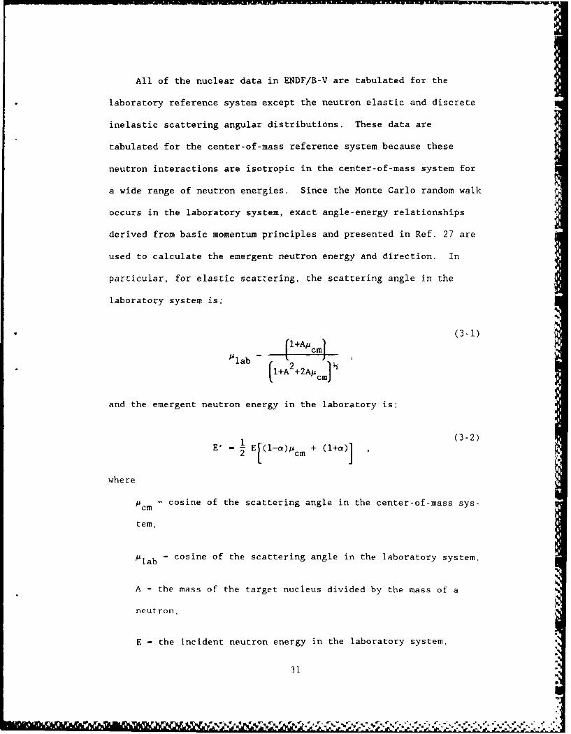
All of the nuclear data in ENDF/B-V are tabulated for the
laboratory reference system except the neutron elastic and discrete
inelastic scattering angular distributions. These data are
tabulated for the center-of-mass reference system because these
neutron interactions are isotropic in the center-of-mass system for
a wide range of neutron energies. Since the Monte Carlo random walk
occurs in the laboratory system, exact angle-energy relationships
derived from basic momentum principles and presented in Ref. 27 are
used to calculate the emergent neutron energy and direction. In
particular, for elastic scattering, the scattering angle in the
laboratory system is:
(3-1)l+Acm]
"lab IL2 j(l+A +2A cm)
and the emergent neutron energy in the laboratory is:
E 1 + (+ )] (3-2)2'- E[(l---a)Pc (14a)
where
Acm = cosine of the scattering angle in the center-of-mass sys-
tem,
Plab = cosine of the scattering angle in the laboratory system,
A = the mass of the target nucleus divided by the mass of a
neutron,
E - the incident neutron energy in the laboratory system,
31
p
- , r-- . zr~ , . .- - . -.-. - ,- -- . -. .-. o -. , . -.- -' -
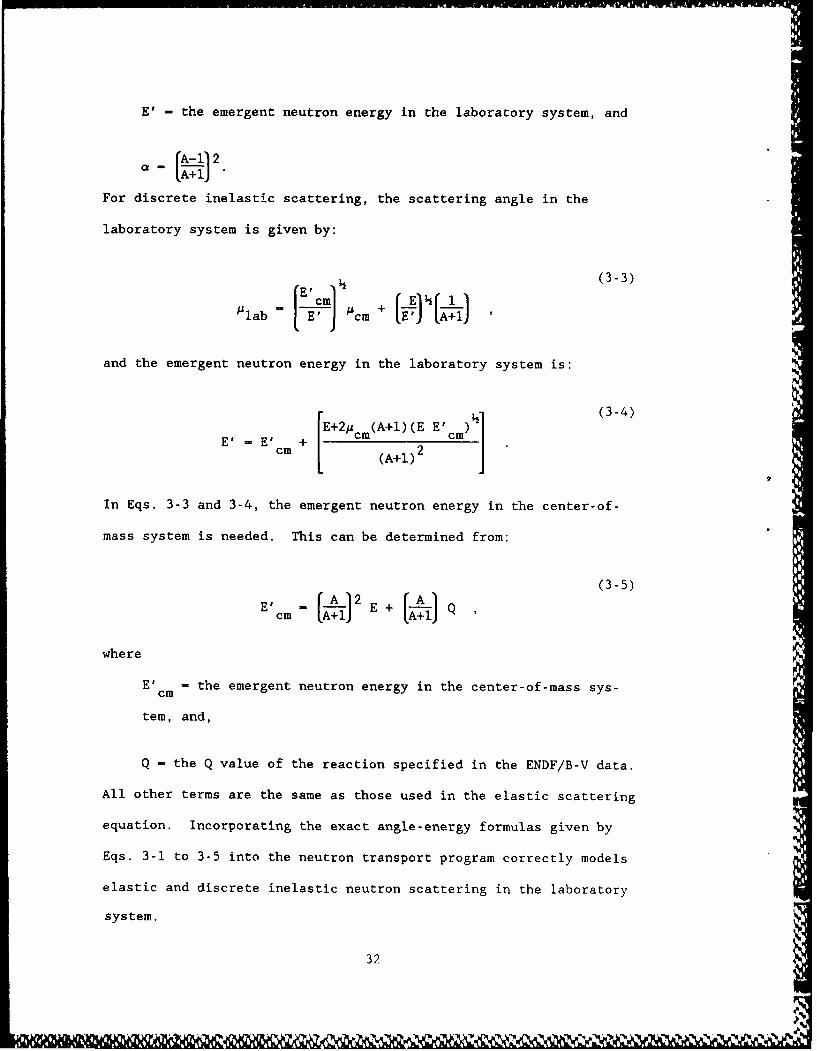
E'- the emergent neutron energy in the laboratory system, and
- (A-l)2
For discrete inelastic scattering, the scattering angle in the
laboratory system is given by:
E' cm (3-3)
~lab I (EJ cm [E'JA_1
and the emergent neutron energy in the laboratory system is:
E+2, cm(A+)(E E'CM) (3-4)
cm + (A+Il)2
In Eqs. 3-3 and 3-4, the emergent neutron energy in the center-of-
mass system is needed. This can be determined from:
(3-5)
cm (A)2 + Q
where
E' - the emergent neutron energy in the center-of-mass sys-cm
tem, and,
Q - the Q value of the reaction specified in the ENDF/B-V data.
All other terms are the same as those used in the elastic scattering
equation. Incorporating the exact angle-energy formulas given by
Eqs. 3-1 to 3-5 into the neutron transport program correctly models
elastic and discrete inelastic neutron scattering in the laboratory
system.
32
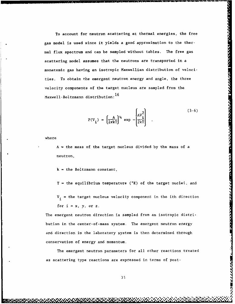
To account for neutron scattering at thermal energies, the free
gas model is used since it yields a good approximation to the ther-
mal flux spectrum and can be sampled without tables. The free gas
scattering model assumes that the neutrons are transported in a
monatomic gas having an isotropic Maxwellian distribution of veloci-
ties. To obtain the emergent neutron energy and angle, the three
velocity components of the target nucleus are sampled from the
Maxwell-Boltzmann distribution: 16
r A 21 (3-6)(( AV.
) rkT) exP-
where
A - the mass of the target nucleus divided by the mass of a
neutron,
k - the Boltzmann constant,
T - the equilibrium temperature (*K) of the target nuclei, and
V. - the target nucleus velocity component in the ith direction
for i - x, y, or z.
The emergent neutron direction is sampled from an isotropic distri-
bution in the center-of-mass system. The emergent neutron energy
and direction in the laboratory system is then determined through
conservation of energy and momentum.
The emergent neutron parameters for all other reactions treated
as scattering type reactions are expressed in terms of post-
33
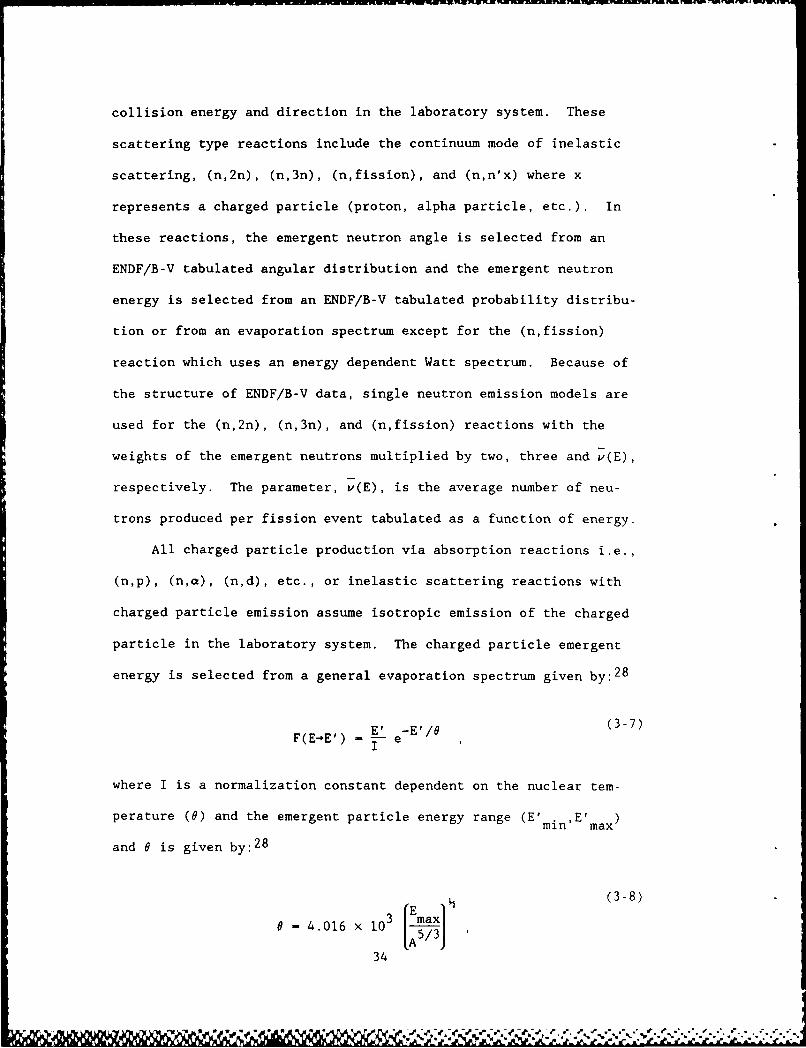
collision energy and direction in the laboratory system. These
scattering type reactions include the continuum mode of inelastic
scattering, (n,2n), (n,3n), (n,fission), and (n,n'x) where x
represents a charged particle (proton, alpha particle, etc.). In
these reactions, the emergent neutron angle is selected from an
ENDF/B-V tabulated angular distribution and the emergent neutron
energy is selected from an ENDF/B-V tabulated probability distribu-
tion or from an evaporation spectrum except for the (n,fission)
reaction which uses an energy dependent Watt spectrum. Because of
the structure of ENDF/B-V data, single neutron emission models are
used for the (n,2n), (n,3n), and (n,fission) reactions with the
weights of the emergent neutrons multiplied by two, three and v(E),
respectively. The parameter, .(E), is the average number of neu-
trons produced per fission event tabulated as a function of energy.
All charged particle production via absorption reactions i.e.,
(n,p), (n,a), (n,d), etc., or inelastic scattering reactions with
charged particle emission assume isotropic emission of the charged
particle in the laboratory system. The charged particle emergent
energy is selected from a general evaporation spectrum given by:2 8
E' -E'/6 (3-7)F(E-E') - I e
where I is a normalization constant dependent on the nuclear tem-
perature (0) and the emergent particle energy range (E' . E' )mln max
and 0 is given by:2 8
3 E ax (3-8)
6 - 4.016 x 10³ /
34
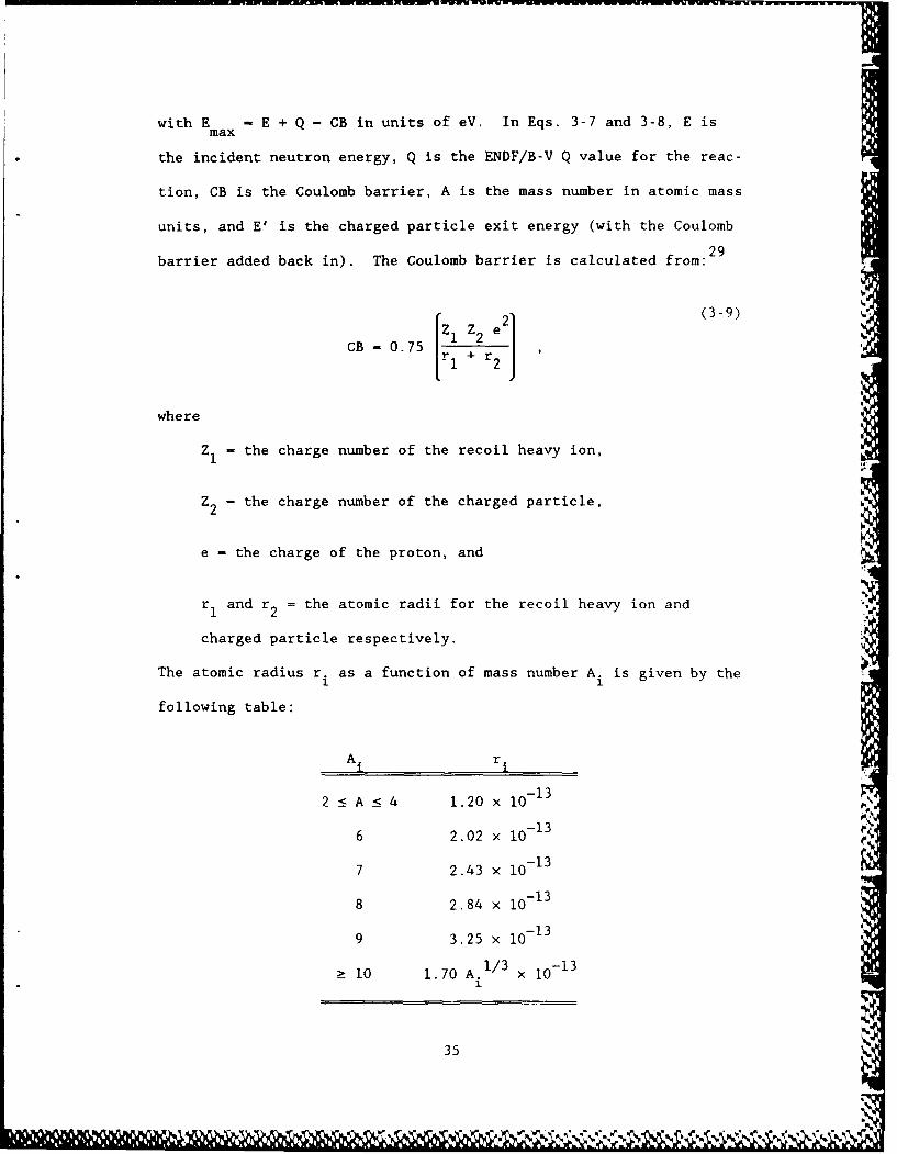
with E - E + Q - CB in units of eV. In Eqs. 3-7 and 3-8, E ismax
the incident neutron energy, Q is the ENDF/B-V Q value for the reac-
tion, CB is the Coulomb barrier, A is the mass number in atomic mass
units, and E' is the charged particle exit energy (with the Coulomb
29barrier added back in). The Coulomb barrier is calculated from:
B - 0.75 z Iz2 e] (3-9)
where
Z - the charge number of the recoil heavy ion,
Z2 - the charge number of the charged particle,
e - the charge of the proton, and
* and r2 = the atomic radii for the recoil heavy ion and
charged particle respectively.
The atomic radius r. as a function of mass number A. is given by the
following table:
A. r.
2 ! A : 4 1.20 x 10- 1 3
6 2.02 x 10⁻¹³
7 2.43 x 10⁻¹³
8 2.84 x 10- 13
9 3.25 x 10- 13
10 1.70 A. 1/3 X 10- 13
1
35
The factor 0.75 is set arbitrarily to account for charged particle
emission below the Coulomb barrier.
All compound nuclei excited through neutron interactions
(except elastic scattering) possess the potential of emitting one or
more photons while decaying to ground state. Therefore, for every
neutron interaction except elastic scattering, a check is made to
determine if secondary photon production data are available. If
there are data available, a photon is produced with a direction
assumed isotropic in the laboratory system, an energy selected from
the ENDF/B-V tabulated distribution, and weight equal to the
ENDF/B-V energy dependent multiplicity. There are some materials
with absorption reactions resulting in ground state transitions.
For these reactions a test is implemented to insure no secondary
photon generation occurs.
The photon production capability is programmed to model the
natural physical processes as accurately as possible. Unfor-
tunately, the photon production data in ENDF/B-V are not well known
for some of the individual neutron interactions in many materials.
Consequently, for these materials, the ENDF/B-V photon production
data have been lumped into one file encompassing the individual neu-
tron interactions which might produce a secondary photon. The neu-
tron transport code utilizes these data to produce a photon whose
direction, energy, and weight are representative average values for
these neutron interactions.
Each neutron interaction produces a recoil heavy ion. In ioni-
zation chamber response analysis, recoil heavy ions can deposit
energy in the active medium thereby contributing to the detector
36
signal. Therefore, the energy and direction of the recoil heavy
ions must be determined for each neutron interaction. This is
accomplished using energy and momentum balances for all incident and
exit particles produced in the collision.
3.2 PHOTON INTERACTIONS
The photoelectric effect, Compton scattering and pair produc-
tion are the three processes considered in the photon transport pro-
gram. In the photoelectric process, a photon is absorbed and an
orbital electron is emitted with approximately all of the energy of
the photon transferred to the electron. The electron is ejected
from its shell with kinetic energy equal to the incident photon
energy less the binding energy of the orbital electron (with a very
small amount of energy taken up by the nucleus). Momentum is con-
served by recoil of the whole atom. The photoelectric process is
the dominant photon interaction for photons with energies below 0.1
MeV. Furthermore, because of momentum and energy conservation con-
siderations, the photoelectric process is more likely to occur with
the more tightly bound K-shell and L-shell electrons.
Compton scattering is the elastic scattering of a photon by an
essentially free electron. The incident photon imparts energy to
the electron and emerges from the collision with a new direction and
energy. In the Compton scattering process, the electrons are
assumed to be free - that is, not bound within the atom or interact-
ing among themselves. The Compton effect becomes important for
incident photon energies greater than 0.1 MeV.
37
In the pair production process, a photon interacts with the
electrostatic field of a charged particle. The incident photon is
completely absorbed resulting in the production of an electron-
positron pair. This photon interaction requires an incident photon
energy of at least twice the resi mass of an electron, i.e., 1.022
MeV, and becomes increasingly more probable as the photon energy
increases above 1.022 MeV. Momentum and energy is conserved in the
process by the recoil of the charged particle. Either the nucleus
or an atomic electron can provide the necessary electrostatic field
for the process. Because of the greater charge of the nucleus, the
interactions are primarily nuclear. If, however, the process occurs
in the field of an atomic electron, energy is transferred to the
recoil electron and a triplet is produced.3 0 The triplet consists
of the recoil electron and the electron-positron pair. Because of
momentum and energy considerations, the threshold energy for triplet
production is four times the rest mass of an electron, i.e., 2.044
MeV.
The interaction cross sections for the photoelectric, Compton,
and pair production processes exhibit a Z dependence. 3 1 The Compton
effect is linearly dependent on the number of electrons per atom and
therefore is proportional to Z. The photoelectric process is pro-
nportional to Z , where n varies from 3 to 5, and diminishes rapidly
with increasing photon energy for any element. The pair production
process is proportional to Z for interaction with atomic electrons
and proportional to Z2 for interactions with the nucleus. However,
only in iron and higher Z materials does the pair production process
account for a significant portion of the energy absorption for
38
incident photon energies below 10 MeV. Consequently, most ioniza-
tion chamber response analysis for photons will be dominated by the
photoelectric and Compton processes. The theoretical and empirical
formulae used to generate the cross sections for the above photon
interactions are presented in detail in Ref. 19.
3.3 ELECTRON INTERACTIONS
Elastic scattering off the nucleus, inelastic scattering off
the atomic electrons, bremsstrahlung production, and positron
annihilation are the electron (and positron) interactions considered
in the photon transport program. As stated earlier, difficulties
arise in electron transport because the cross sections for all the
above interactions (except annihilation) become very large as the
electron energy approaches zero. Therefore, it is not feasible to
simulate every interaction, and they are lumped together and treated
in a continuous manner. Cutoff energies are used to distinguish
between continuous and discrete interactions. Any electron interac-
tion which produces a delta-ray with an energy greater than the
electron cutoff energy or a photon with an energy greater than the
photon cutoff energy is considered a discrete event. All other
electron interactions are treated in a continuous manner giving rise
to continuous energy losses and direction changes to the electron
between discrete interactions.
The continuous energy loss models complicate electron transport
because the cross section varies along the path of the electron and
the electron path is not straight. This complication is rectified
by introducing an additional fictitious interaction which forces the
39
6wrw
total cross section to remain constant along the electron path. If
this fictitious interaction is chosen, the electron experiences a
straight-ahead scattering i.e., no interaction at all. Otherwise,
the interaction is considered real and is dealt with in the usual
manner.
Finally, to account for multiple scattering of the electrons,
the transport of the electron between interactions is divided into
small steps. Within each small step the electron is assumed to fol-
low a straight line, and multiple scattering is accounted for by
changing the electron's direction at the end of each small step.
The size of the steps is kept small enough to insure that the true
electron path length is not much larger than the straight line path
length, and that the angle between the initial and final directions
follows the appropriate angular distributicn.
The above discussion is condensed from material presented in
Ref. 19. As in the case with photon interactions, the theoretical
and empirical formulae used to generate the cross sections for the
above electron interactions are presented in detail in Ref. 19.
3 .4 CHARGED PARTICLE INTERACTIONS
In solving the Boltzmann transport equation for charged parti-
cles, i.e., protons, alpha particles, recoil heavy ions, etc., the
only interactions considered in the present work are continuous
energy loss mechanisms. This is due to the lack of charged particle
cross section data for most materials. To simulate a Monte Carlo
random walk, a very small fictitious transport cross section is
incorporated to determine the next "collision" site. Because this
40
%b
cross section is very small (1.0 x 10⁻¹⁰), the charged particle
transport kernel will almost always provide the distance to the
material boundary as the distance to be transported. Prior to tran-
sport, the particle's range for complete energy loss is calculated
from the stopping power and range/energ, table using the following
32 P
relation:
R(E) _ E dE (3-10)
Ro dE/dx
where
R(E) - the range of a charged particle in a particular medium
with energy dE about E, and,
dEd the stopping power of a particular medium for a charged
particle with energy dE about E.
If the particle's range is less than the distance to the material
boundary, all the particle's energy is assumed deposited in the
material. If the range is greater than the distance to the material
boundary, the stopping power and range/energy table are used to
determine the fraction of energy deposited in the material and the
particle is transported to the material boundary with the remaining
energy. This process is repeated until the particle loses all of
its energy. The theoretical formulae used in the present work for
generating the stopping powers and range/energy tables are given in
Ref. 32.
Recombination effects are sometimes a problem in gas or liquid
ionization chambers. Recombination results from ionized electrons
recombining with charged ions thereby decreasing the charge
41
~ ~" PS~p' ~ VV% V.~.~ !
collected. If recombination effects are significant, the nonlinear-
ity of the charge collected (Q) is taken into account using Birks'
21law:
dE (3-11)
dQ dEdx I+kB-x_
where kB is the recombination constant determined experimentally.
If kB is zero, the charge collected is proportional to the energy
deposited, i.e. In the code system, recombination effectsdx dx"
are computed for each individual particle when they are determined
to be significant. However, in ionization chamber analysis, recom-
bination effects are usually negligible. This formulation for cal-
culating recombination effects was chosen because of the ease of
application to the stopping powers and range/energy tables used in
the charged particle transport.
42
CHAPTER IV
SYSTEM VERIFICATION AND RESULTS
4.0 INTRODUCTION
Accomplishment of the first four objectives outlined in Chapter
I led to the development of MICAP - A Monte Carlo Ionization Chamber
Analysis Package. MICAP is a modular code system designed to calcu-
late the response of an ionization chamber to a mixed neutron and
photon radiation environment. Figure 4-1 depicts a flow diagram of
the overall calculational procedure employed in MICAP. For this
collection of codes, the approach has been to develop a "general"
ionization chamber analysis code system, applicable to a wide range
of problems, through the use of input arrays and user supplied sub-
routines. A user's manual for MICAP is given in Ref. 33 complete
with sample problems for each module.
Establishing the validity of the nuclear models incorporated
into the transport modules of the code system involved implementa-
tion of a five part verification program. The verification program
included comparing results obtained with existing code systems and
comparing with experimental results. Each part of the verification
program investigated a particular aspect of the radiation transport
processes applicable to ionization chamber analysis. More specifi-
cally, the verification program involved:
1. Comparisons with MORSE 17 results to determine validity of
neutron transport, secondary photon production, and photon
transport processes.
43
>4 0U
'00-44
r/2 -
I w ~ O)OZ 81
otz w -4
4
000
ICA.
'4 "
'4
4 Od
cl~mU
0z
*O 4
z 44
l 'o w ' % ~ % - *

2. Comparisons with MACK-IV 34 and RECOIL 3 5 results to deter-
mine validity of nuclear models used to describe indivi-
dual neutron reactions.
3. Comparisons with 05S36 results to determine validity of
charged particle transport processes.
4. Comparisons with experimental results for photon calibra-
tion experiments.
5. Comparisons with experimental results for mixed neutron
and photon radiation experiments.
The remainder of this chapter discusses each part of the verifica-
tion program.
4.1 COMPARISON WITH MORSE
To verify the neutron transport, secondary photon production,
and photon transport processes in MICAP, an iron slab transmission
problem was analyzed with both MORSE and MICAP. The MORSE code sys-
tem was chosen for the comparison because its performance has
already been verified through comparisons with experiments and com-
parisons with other code systems. 1 6 ,1 7 ,37 Consequently, comparisons
with MORSE should provide a reliable indication of the validity of
the neutron transport, secondary photon production, and photon tran-
sport processes in MICAP, The calculations involved modeling a neu-
tron point source incident on the front face of iron slabs having
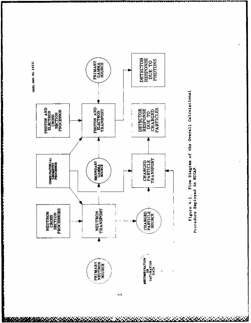
thicknesses 10 and 20 cm. The material parameters for the iron slab
are presented in Table 4-1 and the geometry configuration is shown
in Figure 4-2. Both code systems calculated the neutron and
%'id
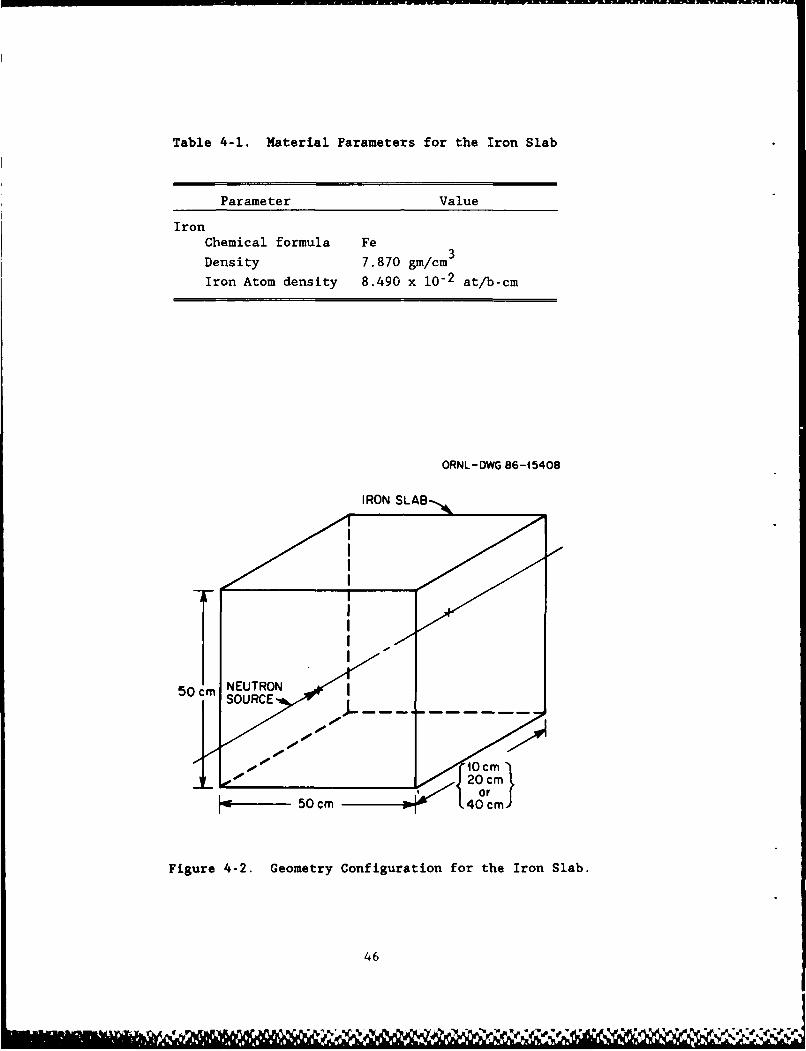
Table 4-1. Material Parameters for the Iron Slab
Parameter Value
IronChemical formula Fe
Density 7.870 gm/cm3
Iron Atom density 8.490 x 10⁻² at/b-cm
ORNL-DWG 86-15408
I R O N S L B , , ,
50 NEUTRON l
loo
50 cmm
H -4 50cm o; 40cml
Figure 4-2. Geometry Configuration for the Iron Slab.
46
LIII, f !
secondary photon leakage spectra out the back face of the iron slab,
and the secondary photon production in the iron slab.
The iron cross section data used in MICAP differed from those
used in the MORSE calculations. MICAP used ENDF/B-V point cross
section data thinned to within a tolerance of 0.1%. The MORSE cal-
culations for the 10 cm iron slab used an ENDF/B-IV 105n-211 cou-
pled, P multigroup library.1 8 To insure different cross section
data bases were not a source of discrepancy, the MORSE calculations
for the 20 cm iron slab used an ENDF/B-V 37n-217 coupled, P3, multi-
group library3 8 as well as the ENDF/B-IV 105n-211 coupled, P3' mul-
tigroup library.
The 10-cm-thick iron slab was analyzed using a mono-directional
point source centered on the front face of the slab and the 20-cm-
thick iron slab was analyzed using an isotropic point source cen-
238 Utered on the front face. Both iron slabs were analyzed using a U
fission spectrum neutron source and a mono-energetic neutron source
(14.2 MeV for the 10 cm slab and 14.0 MeV for the 20 cm slab). The
MORSE calculations used Russian roulette and splitting in the tran-
sport and the MICAP calculations were performed using analog Monte
Carlo. All calculations used 100,000 source neutrons incident on
the iron slab.
The neutron and secondary photon leakage flux spectra out the
back face of the 10 cm iron slab and the secondary photon production
spectra are presented in Figures 4-3 to 4-5 respectively for the
238U fission neutron source. The figures indicate excellent agree-
ment between MICAP and MORSE for the back face leakage spectra and
secondary photon production spectra. The spectral differences seen
47
p.
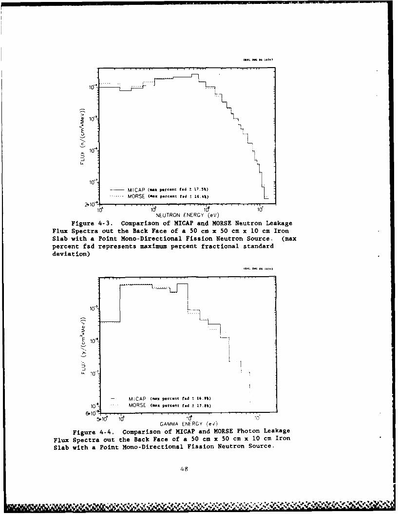
ORML 8M6 141
10-t ....
o-
S107t
MICAP (mAx percent fad +
17.5%)--.---- MORSE (max percent fad _ 16.4%)
21"*''1 10'
NEUTRON ENERGY (eV)
Figure 4-3. Comparison of MICAP and MORSE Neutron Leakage
Flux Spectra out the Back Face of a 50 cm x 50 cm x 10 cm Iron
Slab with a Point Mono-Directional Fission Neutron Source. (max
percent fsd represents maximum percent fractional standard
deviation)
OAL 88G 54 16515
10-t
10-7
MICAP (max percent fad t 16.9%)
10 . MORSE (Sax percent fad ± 17.81)
GAMMA ENERGY (ev)
Figure 4-4. Comparison of MICAP and MORSE Photon Leakage
Flux Spectra out the Back Face of a 50 cm x 50 cm x 10 cm Iron
Slab with a Point Mono-Directional Fission Neutron Source.
48
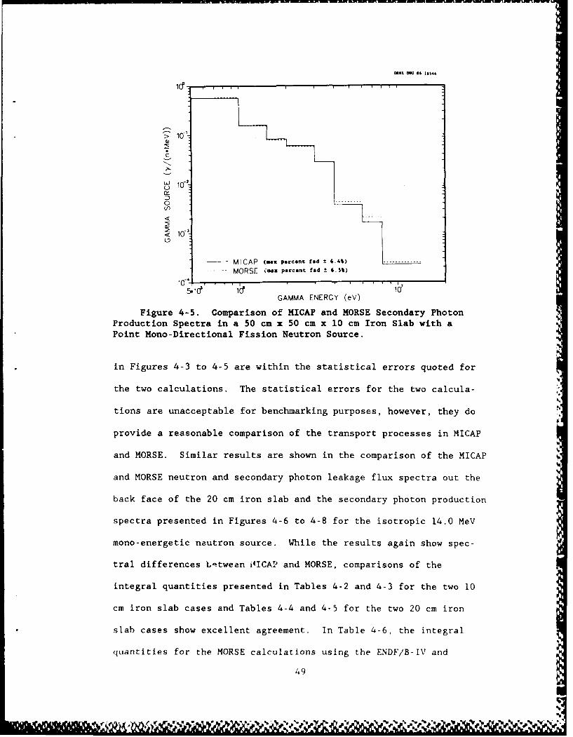
idd
V)
<
0
< 10
0
MICAP (max percent fad ± 6.41) - ------------
- MORSE (ax percent fad ± 6.5%)
10-0
GAMMA ENERGY (eV)
Figure 4-5. Comparison of MICAP and MORSE Secondary PhotonProduction Spectra in a 50 cm x 50 cm x 10 cm Iron Slab with aPoint Mono-Directional Fission Neutron Source.
in Figures 4-3 to 4-5 are within the statistical errors quoted for
the two calculations. The statistical errors for the two calcula-
tions are unacceptable for benchmarking purposes, however, they do
provide a reasonable comparison of the transport processes in MICAP
and MORSE. Similar results are shown in the comparison of the MICAP
and MORSE neutron and secondary photon leakage flux spectra out the
back face of the 20 cm iron slab and the secondary photon production
spectra presented in Figures 4-6 to 4-8 for the isotropic 14.0 MeV
mono-energetic neutron source. While the results again show spec-
tral differences L-tween iOICA? and MORSE, comparisons of the
integral quantities presented in Tables 4-2 and 4-3 for the two 10
cm iron slab cases and Tables 4-4 and 4-5 for the two 20 cm iron
slab cases show excellent agreement. In Table 4-6, the integral
quantities for the MORSE calculations using the ENDF/B-IV and
49
(V * C '! % %~ w e %~.~J' ,p ~ e1%w I
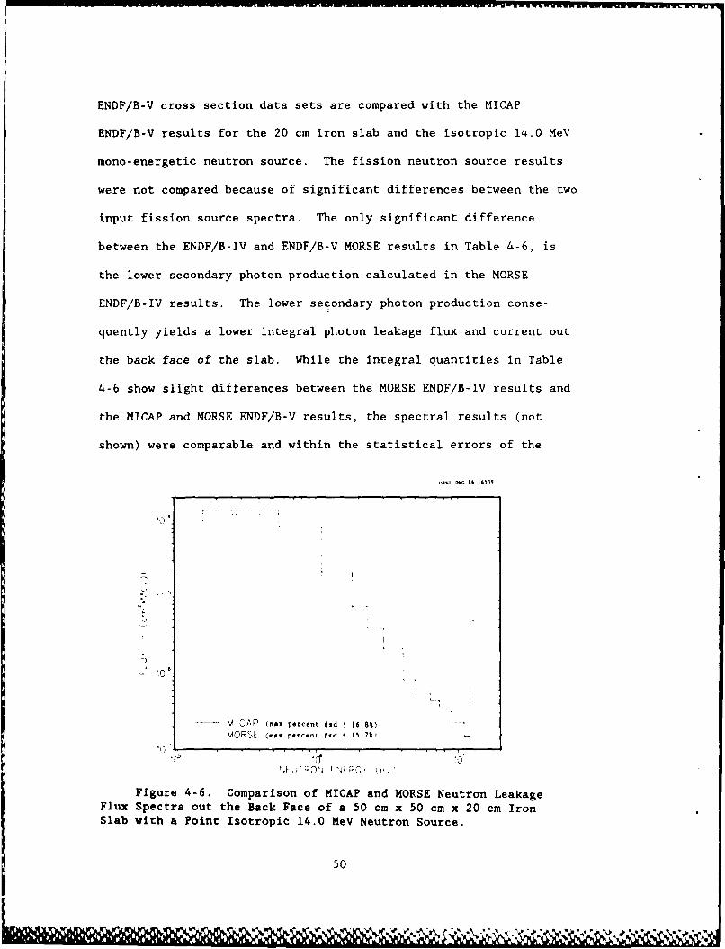
ENDF/B-V cross section data sets are compared with the MICAP
ENDF/B-V results for the 20 cm iron slab and the isotropic 14.0 MeV
mono-energetic neutron source. The fission neutron source results
were not compared because of significant differences between the two
input fission source spectra. The only significant difference
between the ENDF/B-IV and ENDF/B-V MORSE results in Table 4-6, is
the lower secondary photon production calculated in the MORSE
ENDF/B-IV results. The lower secondary photon production conse-
quently yields a lower integral photon leakage flux and current out
the back face of the slab. While the integral quantities in Table
4-6 show slight differences between the MORSE ENDF/B-IV results and
the MICAP and MORSE ENDF/B-V results, the spectral results (not
shown) were comparable and within the statistical errors of the
.AWL DW I6 16539
104
M-'AP (max percent fad 16S6%)
MOPSE (max percent fsd t 15,71'
Figure 4-6. Comparison of MICAP and MORSE Neutron LeakageFlux Spectra out the Back Face of a 50 cm x 50 cm x 20 cm IronSlab with a Point Isotropic 14.0 MeV Neutron Source.
50
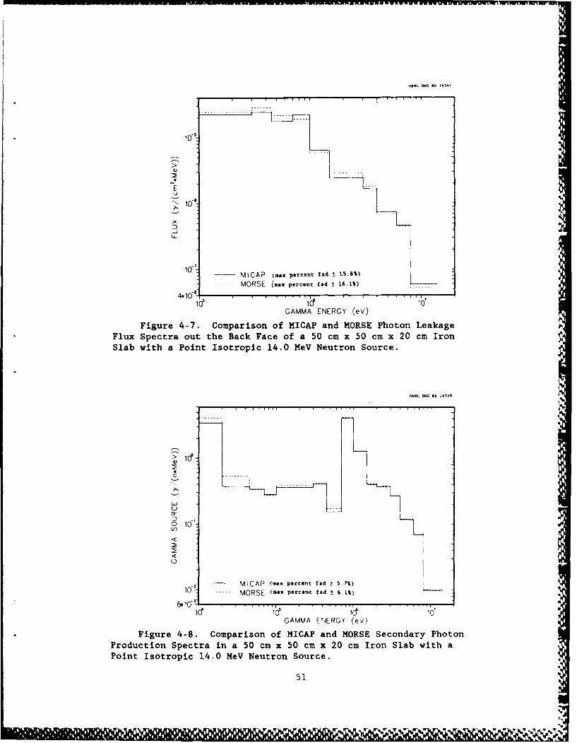
OPNL DWG 96 16541
IE'-
10 MICAP (max percent fsd ± 15.6%)
----MORSE (max percent fsd ± 16.1%)-----
4*10- *''1 0
GAMMA ENERGY (eV)
Figure 4-7. Comparison of MICAP and MORSE Photon LeakageFlux Spectra out the Back Face of a 50 cm x 50 cm x 20 cm IronSlab with a Point Isotropic 14.0 MeV Neutron Source.
0 1ff-,
C
M A mxprcn a .%10(O S ma ecn fdt6 %
GAM a-RY(v
PitIorpc10 . MORS (eutro pertce .t
6'10
GV M WiRG (eV S111 P
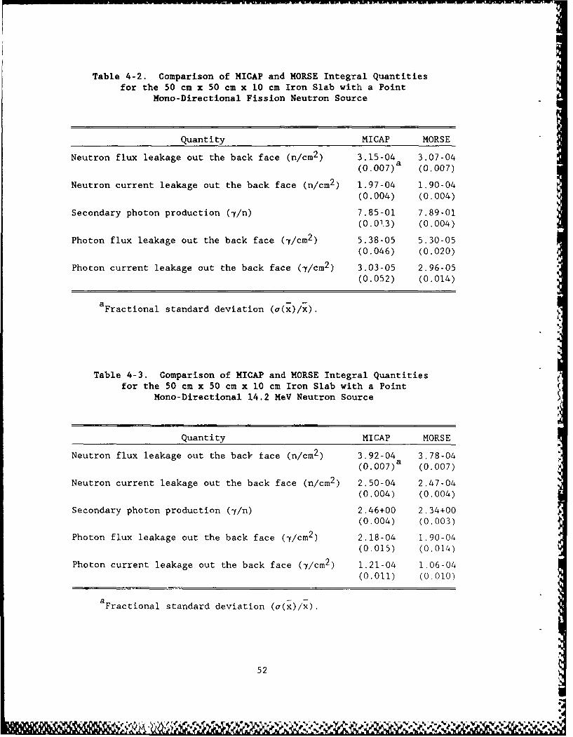
Table 4-2. Comparison of MICAP and MORSE Integral Quantitiesfor the 50 cm x 50 cm x 10 cm Iron Slab with a Point
Mono-Directional Fission Neutron Source
Quantity MICAP MORSE
Neutron flux leakage out the back face (n/cm2 ) 3.15-04 3.07-04(0.007) (0.007)
Neutron current leakage out the back face (n/cm2) 1.97-04 1.90-04(0.004) (0.004)
Secondary photon production (7/n) 7.85-01 7.89-01(0.01.3) (0.004)
Photon flux leakage out the back face (7/cm2 ) 5.38-05 5.30-05(0.046) (0.020)
Photon current leakage out the back face (7/cm2 ) 3.03-05 2.96-05(0.052) (0.014)
aFractional standard deviation (a(x)/x).
I-
Table 4-3. Comparison of MICAP and MORSE Integral Quantitiesfor the 50 cm x 50 cm x 10 cm Iron Slab with a Point
Mono-Directional 14.2 MeV Neutron Source
Quantity MICAP MORSE
Neutron flux leakage out the back iace (n/cm2) 3.92-04 3.78-04(0.007) (0.007)
Neutron current leakage out the back face (n/cm2 ) 2.50-04 2.47-04(0.004) (0.004)
Secondary photon production (7/n) 2.46+00 2.34+00(0.004) (0.003)
Photon flux leakage out the back face (7/cm2 ) 2.18-04 1.90-04(0.015) (0.014)
Photon current leakage out the back face (y/cm2 ) 1.21-04 1.06-04(0.011) (0.010)
aFractional standard deviation (a(x)/x).
52
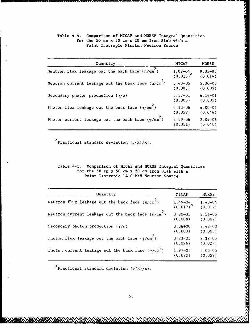
Table 4-4. Comparison of MICAP and MORSE Integral Quantitiesfor the 50 cm x 50 cm x 20 cm Iron Slab with a
Point Isotropic Fission Neutron Source
Quantity MICAP MORSE
Neutron flux leakage out the back face (n/cm ) 1.08-04 9.05-05(0.013)a (0.014)
Neutron current leakage out the back face (n/cm ) 6.43-05 5.30-05(0.008) (0.005)
Secondary photon production (1/n) 5.57-01 6.14-01
(0.006) (0.005)
Photon flux leakage out the back face (-/cm ) 4.33-06 4.80-06(0.058) (0.046)
2FPhoton current leakage out the back face (7/cm ) 2.59-06 2.84-06
(0.051) (0.040)
Fractional standard deviation (a(x)/x).
Table 4-5. Comparison of MICAP and MORSE Integral Quantitiesfor the 50 cm x 50 cm x 20 cm Iron Slab with a
Point Isotropic 14.0 MeV Neutron Source
Quantity MICAP MORSE
Neutron flux leakage out the back face (n/cm ) 1.49-04 1.43-04(0.017) (0.012)
Neutron current leakage out the back face (n/cm ) 8.80-05 8.56-05(0.008) (0.007)
Secondary photon production (7/n) 3.36+00 3.43+00(0.003) (0.003)
Photon flux leakage out the back face (7/cm ) 3.23-05 3.38-05(0.026) (0.027)
Photon current leakage out the back face (7/cm ) 1.97-05 2.C5-05(0.022) (0.022)
Fractional standard deviation (a(x)/x).
53
- .~ .%~ %.*~*~% '~ V~'~ V ~ - % .5-% '
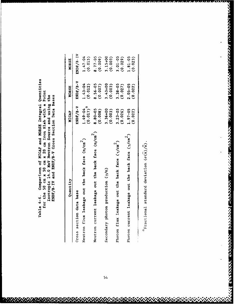
0 0un 00 OC)% 00nC)% 0 c)1l I-4 ' 0 + 0 1 C-4 csj
r, N r- F0 u.0 0 -4 .00 -z r, -4 - 0 -.~ 0 *0 C*.0 0 * 0
I4 1 -:r L 0 e% Un IAn4.) go 0 C'j 0f- 0 cn O r- 0 C4
-AC/ 1 g-4 1 0 + 0 1 N 0c44.) 4.) cn 0~ %' 0 c00 0 LO 0~o -1400 rAz 0 0 0 -0 *0
0' P4 4.) ca
00 4u (A4) no or- 0 G 0C O'0 0 0C-404) "4 N3 I. -4 10 + 0 1e' C i 1 0
41) : C. 00 %D0 (n O r-O000H - 0* CN- *0'
z * 0 * 0 *0 0 *0Ndc 0p -4'-'. 00'.. en'.. cnd .. 4
N$4 0 C4
C.,4$ 0 C',4
$4% UU
41) N1- 4 U co' U- I
' 104. i 03 44
044 >0d0 tj U)4 c mr
X:0 4. d 4 U 0.0 .% Ud 0~0 N 0 .0 ,0 01
to 0 0) U co
0 0g 4) -4to) 1 4-) 4J 0.o u>4.) 0J . 4.) 10
ig A0 4.) H. 0 c0 0 04 0 -A 4) V 10
04)1 ) 0 go r. 4.4 0 'U0'1 c 0 0 4) 0 4 00
.)4 u0 m0 0 0 0 0 "A 0N 0 0 cd 0 4 .
0 0 01 (A. Zc a) 1 oo4 4.) Cd 4) 0o to
04. 0 d 0m 4 -4(D 0 W. 0 co co
.0 4 r 41 0) 4.)00or 0 .-4 0
E-4 04 M~0*
4.) r4 V $4uU 4-4 U ', .4 m0) $4 4-4 UC c co0
0 0 "0wo w4 z4 0 041) 41J 0 4 -j4.
$40 0 : 0 0C .C.) Q) 4) U2
54
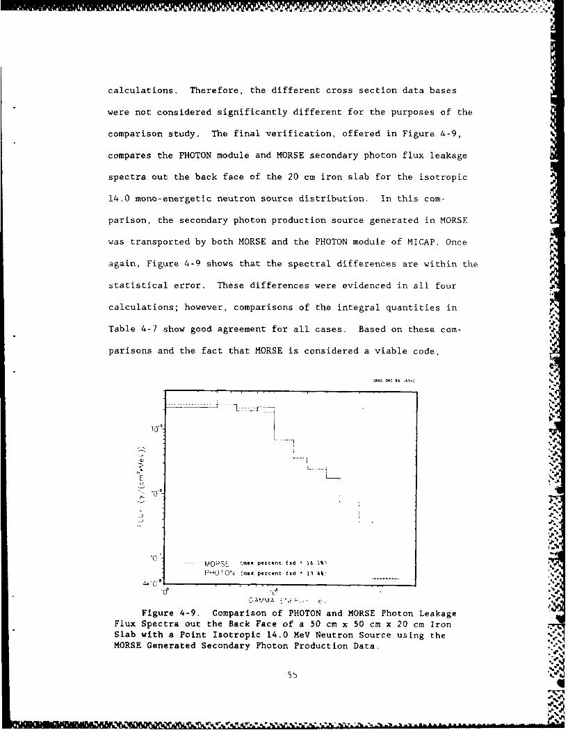
calculations. Therefore, the different cross section data bases
were not considered significantly different for the purposes of the
comparison study. The final verification, offered in Figure 4-9,
compares the PHOTON module and MORSE secondary photon flux leakage
spectra out the back face of the 20 cm iron slab for the isotropic
14.0 mono-energetic neutron source distribution. In this com-
parison, the secondary photon production source generated in MORSE
was transported by both MORSE and the PHOTON module of MICAP. Once
again, Figure 4-9 shows that the spectral differences are within the
statistical error. These differences were evidenced in all four
calculations; however, comparisons of the integral quantities in
Table 4-7 show good agreement for all cases. Based on these com-
parisons and the fact that MORSE is considered a viable code,
NS.
10-
E K'U
O-- PSE (max percent fid 4 16l V
P Q407 0% (max percent fsd - 13 6%) . "
4.10 .,
Figure 4-9. Comparison of PHOTON and MORSE Photon LeakageFlux Spectra out the Back Face of a 50 cm x 50 cm x 20 cm IronSlab with a Point Isotropic 14.0 MeV Neutron Source using theMORSE Generated Secondary Photon Production Data.
55 "%
es
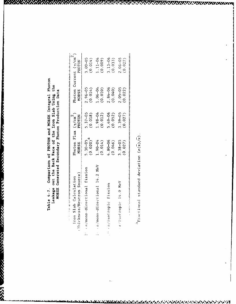
u )z 0 - 00 ON~ 0 c',0 1 j-4 10 1c C-
0- 0 C0 -4 0 C)C
C)0 0 . C) C
0 1-4
0 0 0L0 0 c
914 '0 D0 40 0 C)
Cdr.i 0 0 0", -0- *0$4 ~ *44z .0 *0 .0
4 0
(A 0 C14N Z 0 0 C OC14 OC' 0 r~n 0 C-0 1 4 1 -1 1 un 1 C-414 Q -4 r-0 C)00 0o'0 m o
o 04 P. -0 a') 4 - cw? = *.0 0 > 0 . 0
H0 . 04 u 4X0.0
z 00 04 0' ho 44 0 ** I' I '- 1 (N I-0 0 Ps~ 00 00 00 r
P4u V 0 0 c') - a%- 00 - .n - tCd r. 4 . 0 -C -CD -C
1% 4) 0U OW -.4
w~4 4) r- -40) 10 >
vi -1 -4Q
Cf W -1 0:3 -- 4 :$ (
0 0V' 41 0 C .cov 0 0
-4-
C: C C
the neutron transport, secondary photon production, and photon traTi-
sport processes in MICAP are considered valid.
4.2 COMPARISON WITH MACK-IV AND RECOIL
The neutron and photon leakage flux spectra and secondary pho
ton production spectra presented in the last section demonstrated
the validity of the radiation transport processes The comparior-.
however, did not verify all aspects of the nuclear models usedr
describe the individual neutron reactions important to ioniza" ;'',
chamber response analysis. More specifically,. verification i.,
needed for the nuclear models describing the energy transfer fr,,'
the neutron to the reaction products for all partial cross se*'i..
used in MICAP. To accomplish this goal. a problem consistirn. -t
mono-directional 14.2 MeV mono-energetic neutron! source i:t ider"
a 40-cm-thick iron slab was calculated using, MV"AP The, ma'.-,.
parameters and geometry configuration were the %ame as,,
the spectral comparisons. The MICAP calcula-i,, ,,ns
neutrons and set an energy cut-off at 1.,' 4 '. °, .,v
collisions. The 40-cm-thickness of iron ..- ,. -i t
insured an adequate number of source intr..
charged particles and recoil heavv ios .. ,. -
module were processed in the HEAVY mod,, . .
kinetic energies of the charged par" i. .
duced by the individual neutron r.-ac ,
energies calculated in program HEA'.Y w,:,
appropriate cross sections i, 1,
for the individual neutron reactions. These average kinetic ener-
gies and kerma factors were then compared to results obtained with
MACK-IV 34 and RECOIL.3 5
The kerma factor comparisons involve using microscopic cross
section data evaluate- at 14.2 MeV. Because MACK-IV and RECOIL use
ENDF/B-IV cross section data and MICAP uses ENDF/B-V cross section
data, the microscopic cross sections for the individual neutron
reactions used in all three programs are presented in Table 4-8 As
seen in Table 4-8. there are considerable differences in some of the
cross sections. Thc cross section differences between MACK-IV and
MICAP are attributed to differences in the cross section data bases
,ENDF/B-IV versus ENDF/B-V) and to the energy weighting models used
,o create the MACK-IV multigroup cross section set The differences
between MACK-iV and RECOIL are primarily attributed to differences
ir cross section processing models
The results of the average kinetic energy and kerma factor cal-
,,t ions performed in MICAP show good agreement with results fr,m
MACY TV. ind RECOIL. The comparison with MACK-tV Table , '4 lumps
tie !P, oi nu n1, lejs and harged parti-ie resu1t% for a Pairiculat
h* ' e her "dh-ras "he eimpari -n i th RPYr)' " Tahl , '
i -- '- *1' . .. * ' ? 4h ' '' :' .'* . ' . .* '.- *.% e' ~
AI ff 4' f ; 4 ; * , P , re 911
,. - 9~4 ' 4 ,~#
%
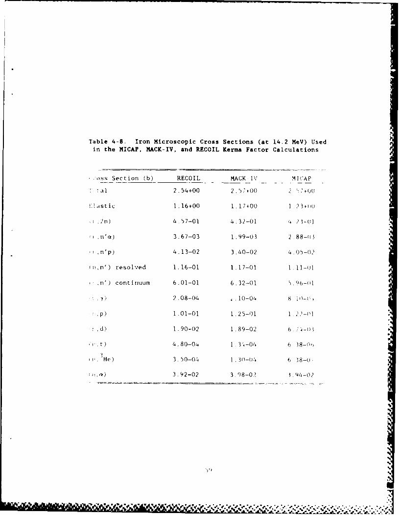
Table 4-8. Iron Microscopic Cross Sections (at 14.2 MeV) Usedin the MICAP, MACK-IV, and RECOIL Kerma Factor Calculations
;Oss Section (b) RECOIL MACK-IV MICAP
' :al 2.54+00 2.57+00 2 <'+Ou
K.:astic 1.16+00 1.17+00 1 23+14)
2n) 4.57-01 4.32-01 4.2 -01
n't 3.67-03 1.99-03 2.88-43
n'p) 4.13-02 3.40-02 4.05-02
,iin') resolved 1.16-01 1.17-01 1.11-0,
.[n') continuum 6.01-01 6,32-01 ).16-01
)) 2.08-04 1.10-04 8. I 0-( 4
.p) 1.01-01 1.25-01 1 2-"10.I
, ) 1.90-02 1.89-02 6., .- ()
* , t) 4.80-04 1. 31-04 6 38-06
1, He) 3.50-04 1. 30-014 6 18--u
, Y) 3.92-02 3.98-0.) 3.44-02
%
5%
,%
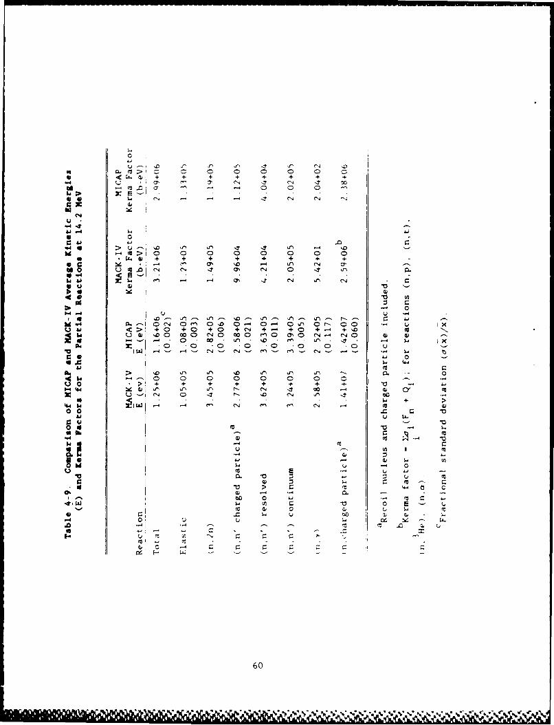
CL t 0 0 0 0 C 0L <L. dj+ + + + + + + +
(7 a,~ C4 41 (j 41 or
06~~C1 C1-4 N N (
-x 4
.4 -S
4 m 0 0 0 0 0 0 0 0. .L w + + + + +- + + +
-4 .' a, 1-0 -4 Ln (N a,
bO'ON UC0 In (N 4 ' (N 040u
4- -D A'j(N ~ (
.1~~~~- 0w C 4C
4w < + 0 + 0 + 0 + (N + +0 +~- cc Ni 4) 10 C)0 0 '0 (NO 0 0 C)en0 (7,0 CN (NOC w 0)
*o 0 , c o an *o . " .-
Aj 0w~ 44.4
04 '0 Pr) '0) m- 0-~ 0 0 0 0 0 0 0 0> + + + + + + + + V -
X44 j45 Lr In fl- CN 41 D .- 4 CY
C 14 +1 r
-4 n '' c14,
-41
-4 (
U (0
U. '- - 3-Obdw 1-.-
tv w m-X~4-
4)~ u -'-
co-~~@4 4) . ... 40
-~~ a~60 C
S. "k %( %N
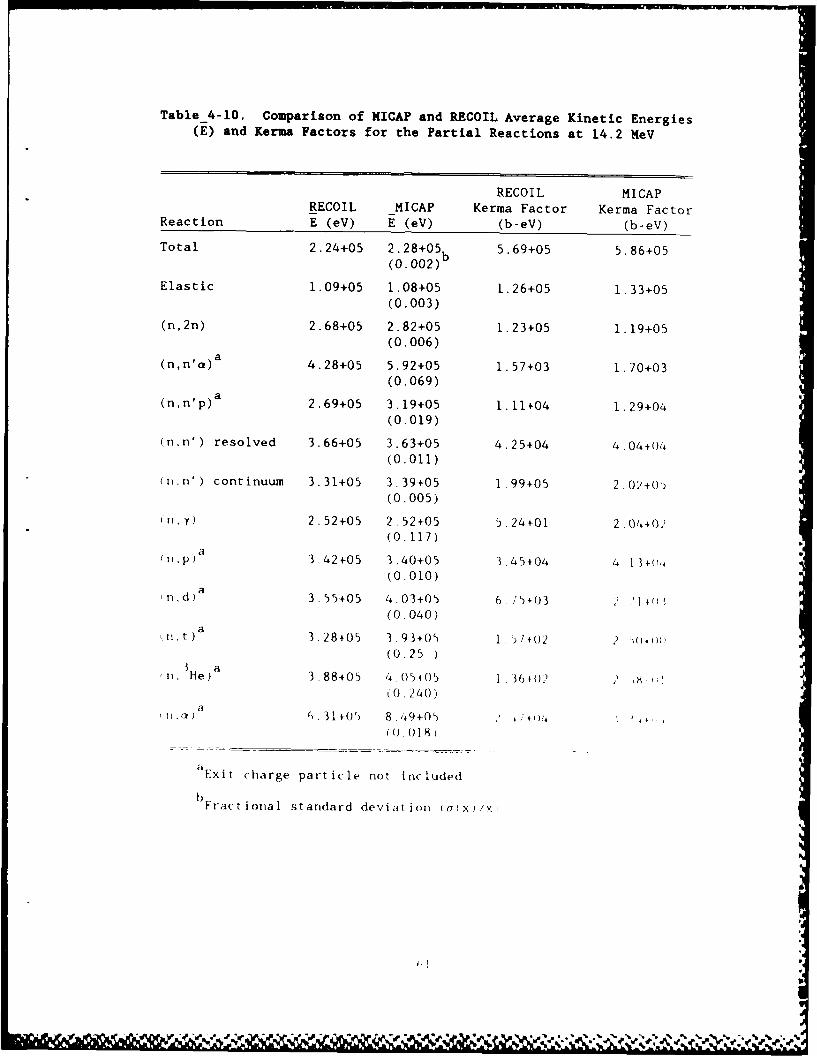
Table_4-10. Comparison of HICAP and RECOIL Average Kinetic Energies(E) and Kerma Factors for the Partial Reactions at 14.2 MeV
RECOIL MICAPRECOIL _MICAP Kerma Factor Kerma Factor
Reaction E (eV) E (eV) (b-eV) (b-eV)
Total 2.24+05 2.28+05 5.69+05 5.86+05
(0.002)b
Elastic 1.09+05 1.08+05 1.26+05 1.33+05(0.003)
(n,2n) 2.68+05 2.82+05 1.23+05 1.19+05(0.006)
(n,n'a) 4.28+05 5.92+05 1.57+03 1.70+03(0.069)
(n,n'p) 2.69+05 3.19+05 1.11+04 1.29+04
(0.019)
(n,n') resolved 3.66+05 3.63+05 4,25+04 4.04+04
(0.011)
(nn') continuum 3.31+05 3.39+05 1.99+05 2.02+0
(0.005)
2.52+05 2.52+05 5,24+01 2.04+02(0.117)
PIp) 3.42+05 3.40+05 3.45+04 4 1+(11.(0.010)
an d) 3.55+05 4.03+05 6 ,5+03 2 '1(0.040)
1 t a 3.28105 3.93+05 1 s 2 1+ 2 )(
(0.25 )3e an, He) 3.88405 4 05+05 136+02 + 0,
(0 240)
T1.) .31+ 8 14++0 8 49+M 4 (),
(0 018)
aExit charge particle not included,
bFractional standard deviation (Q(x)/x
a,
Y'..P e. .'r - ' . 9% % V~~~ib
results are seen in Table 4-10. In general, the nuclear models used
in MICA? to describe the individual neutron reactions are adequate
for calculating ionization chamber responses. The principal differ-
ences noted above are due to different cross section data bases and
cross section processing techniques.
4.3 COMPARISON WITH 05S
In the last section, verification of thE nuclear models used to
describe the individual neutron reactions was described. In
essence, this procedure verified the charged particle and recoil
heavy ion source generation processes in program NEUTRON in much the
same way as the comparisons to MORSE verified the secondary photoni
production processes. The charged particle and recoil heavv ion
transport processes in program VIKAVY, however, remain to be veri
tied. To accomplish this task, a comparison to (,S6was made i'
is a specialized Monte Carlo code for calciilat ing pul se ill ight Ai"
trihut ions due to mono-energet ic nieut ron% inlC ideTIt uI)I 0I Y~til .k IV
riilators W) S i S SpeC ial iZted illn hilt t he odll 11If It'l IT' 1'
14 rho t)I Iy h lt o ge'ti (r Y ri1i c , ompotiiids % . i I I (I-u I 'c1" i Y k . I
V I i( I -', r, W j i- f ili-th -ti ei I e~ i( T e-d ill Ile ' ith~ b i ITI ti -if.
I cii I ( iS 0 I tli i I I I t i I .p 1 1 .e de 1 tt 't*
S tidl Mil AP wwcild II tie I! ',
htIa y i I fl llim i t tni,uie j i f I I I I I il' HI ,\ '
la I. e ..
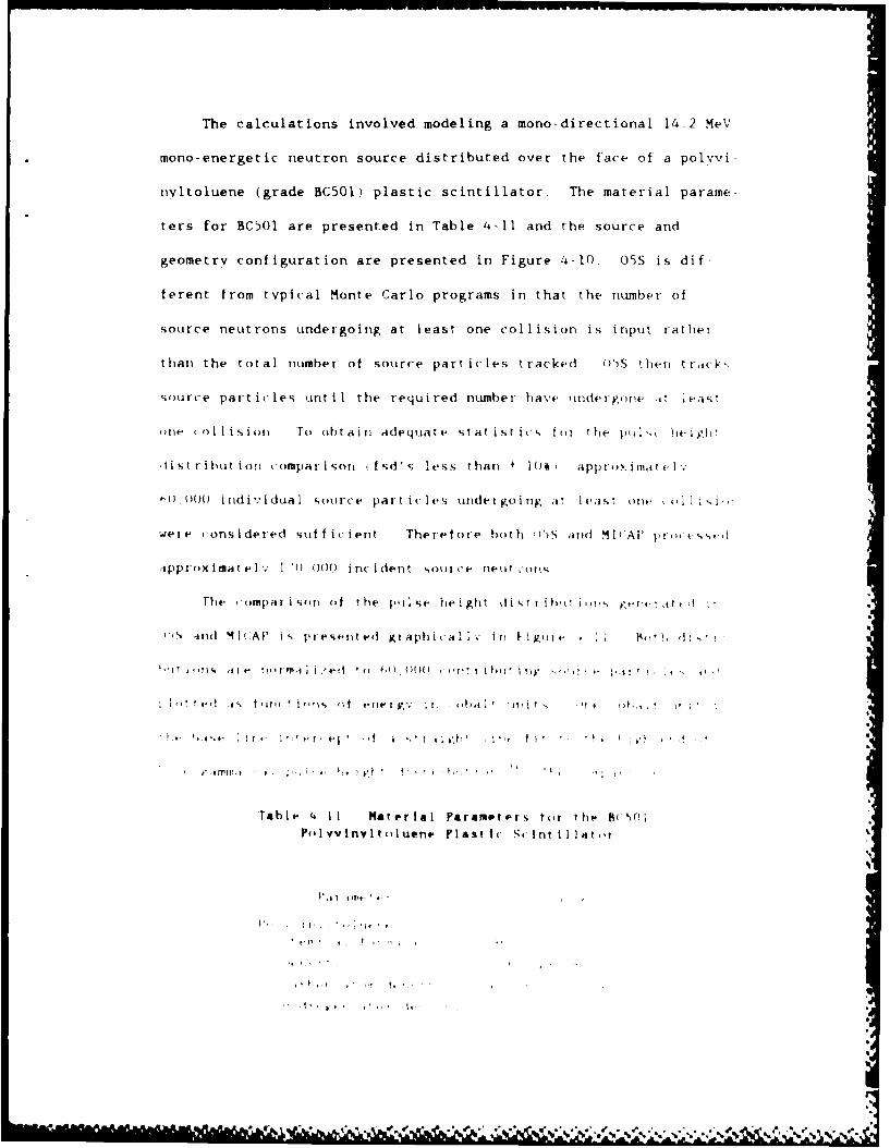
The calculations involved modeling a mono-directional 14.2 MeV
mono-energetic neutron source distributed over the face of a polvvi-
nyltoluene (grade BC5OL) plastic scintillator. The material parame-
ters for BC501 are presented in Table 4-il and the source and
geometry configuration are presented in Figure 4-10. 05S is dif-
ferent from typical Monte Carlo programs in that the number of
source neutrons undergoing at least one collision is input rather
han the total niumber of source particlIes tracked O'is !hen t rack.-
'iource part icl1es unt il the required number- have unde rgone it ea".
"fit Co0i1 is ioil To obtain adequate stat ist ics- for the pkil,- htei~ji,
'listriht ion, comparisoni . fsd.'% less thani * 1* )approximatt IlV
6i( 000 irjdi'id%.al source Part ic le% undeigoing at leas, oiw, olI
wer-e considered sot f i(i jent Therefore both WS awd Ml( ' pi-sst
atpprox imat clv 1 '0) O() inc idenit Sourc(e tictit onst,
The .:ompat i~ori of the plle height ktistl ihbr i-r. e~vr'(' aitt d
arid M1(~ MIAP is Piested( KjAPhiCal 1 ' in, iWir.0 1 Bof I h d
Table 4 It Material Parameter% toy rb the oPolyvlnyltoluen. Plas1 tcS it rlI II to
JrI
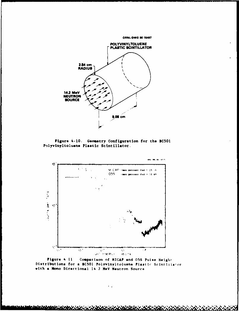
ONL-DWO UN1"07
POLYVINYLTOLUENEPLASTIC SCINTILLATOR
14.2 ht.VNEUTRONi 01
5.06 C'm
Figure 4-10. Geometry Configuration for the ICS01Polyvinyl toluene Plastic Scintillator.
Id C AP (*A percent f@4 10 IA
05S me. percent fid '0 6
Figure 411~ Comparison of MICA? and 05S Pulse HeightDistributions for a B501 Polv'vinyltoluene Plastic Sctntlilaorwith a Mono Directional 14, 2 11eV Neutron Source
' ' ~ "
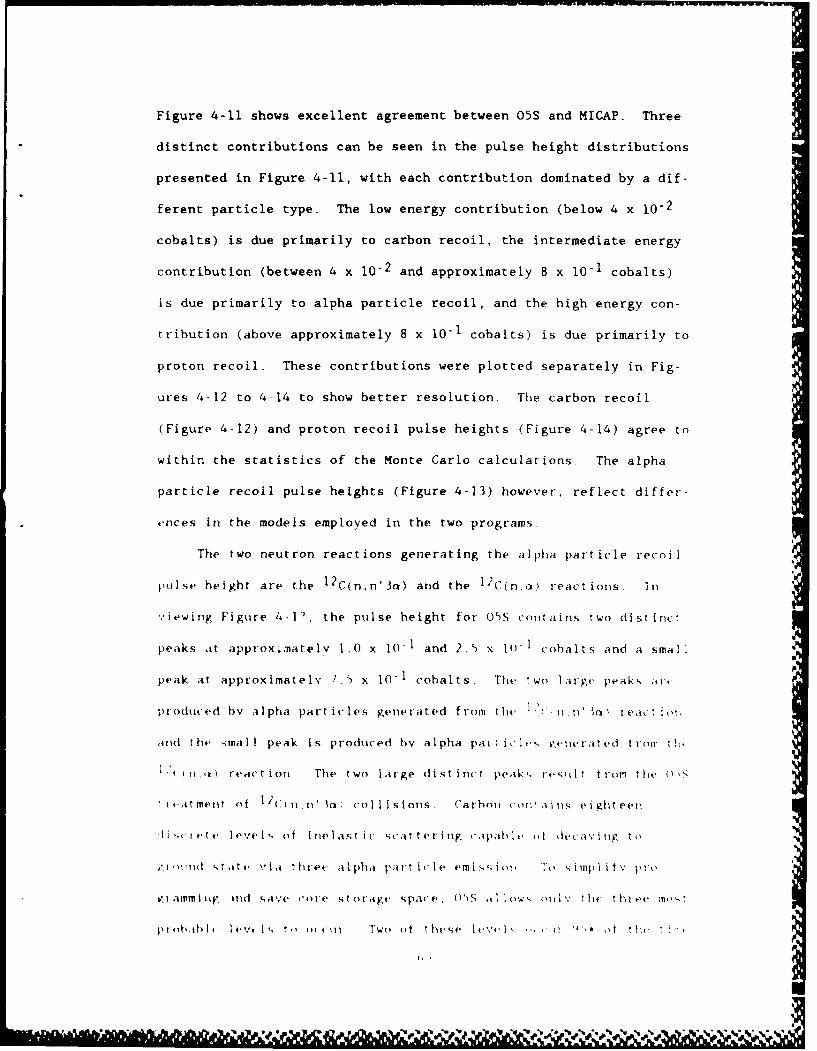
Figure 4-11 shows excellent agreement between 05S and MICAP. Three
distinct contributions can be seen in the pulse height distributions
presented in Figure 4-11, with each contribution dominated by a dif-
ferent particle type. The low energy contribution (below 4 x 10⁻²
cobalts) is due primarily to carbon recoil, the intermediate energy
contribution (between 4 x 10⁻² and approximately 8 x 10⁻¹ cobalts)
is due primarily to alpha particle recoil, and the high energy con-
tribution (above approximately 8 x 10⁻¹ cobalts) is due primarily to
proton recoil. These contributions were plotted separately in Fig-
ures 4-12 to 4-14 to show better resolution. The carbon recoil
(Figure 4-12) and proton recoil pulse heights (Figure 4-14) agree to
within the statistics of the Monte Carlo calculations. The alpha
particle recoil pulse heights (Figure 4-13) however, reflect differ-
ences in the models employed in the two programs.
The two neutron reactions generating the alpha particle recoil
pulse height are the 12 C(n.n'3a) and the 12C(n.a) reactions. In
viewing Figure 4-1 ' the pulse height for OS contains two distinct
peaks at approxamatelv 1.0 x 10 1 and 2.5 x 10 - 1 cobalts and a small
peak at approximately 1.5 x 1(1 cobalts. The two large peak, ,ilt.
produced by alpha particles generated from the 1.'(*'1,1 lo( react i ,o
,id the small peak is produced by alpha part ic t,. rgetiezated t'orn" ti,
I*'( I., ) react ion The two large distinct peak-, rv.xrlt trom the (),s
" ,*.itmentr of 12C(.ton' 3m collisions. Carhot ' r,iins 'ighteell
,li ;¢rete level'; of inlelastic scatteri ng Crapabhl, ot deca%'it to
k'toltlld 't atu e 'ia three alpha particle emis';ior Fo Si rpli t plo
rammillr. Ind save cole storag . spacO, ()s all o'.s- ni'. thc th vet' 11)-.
ptobabl , lv, ti) o'ct11 Two of tl "';e tv '- .. i '0 t ! ' 'i",
'. ,*wJ,' '5
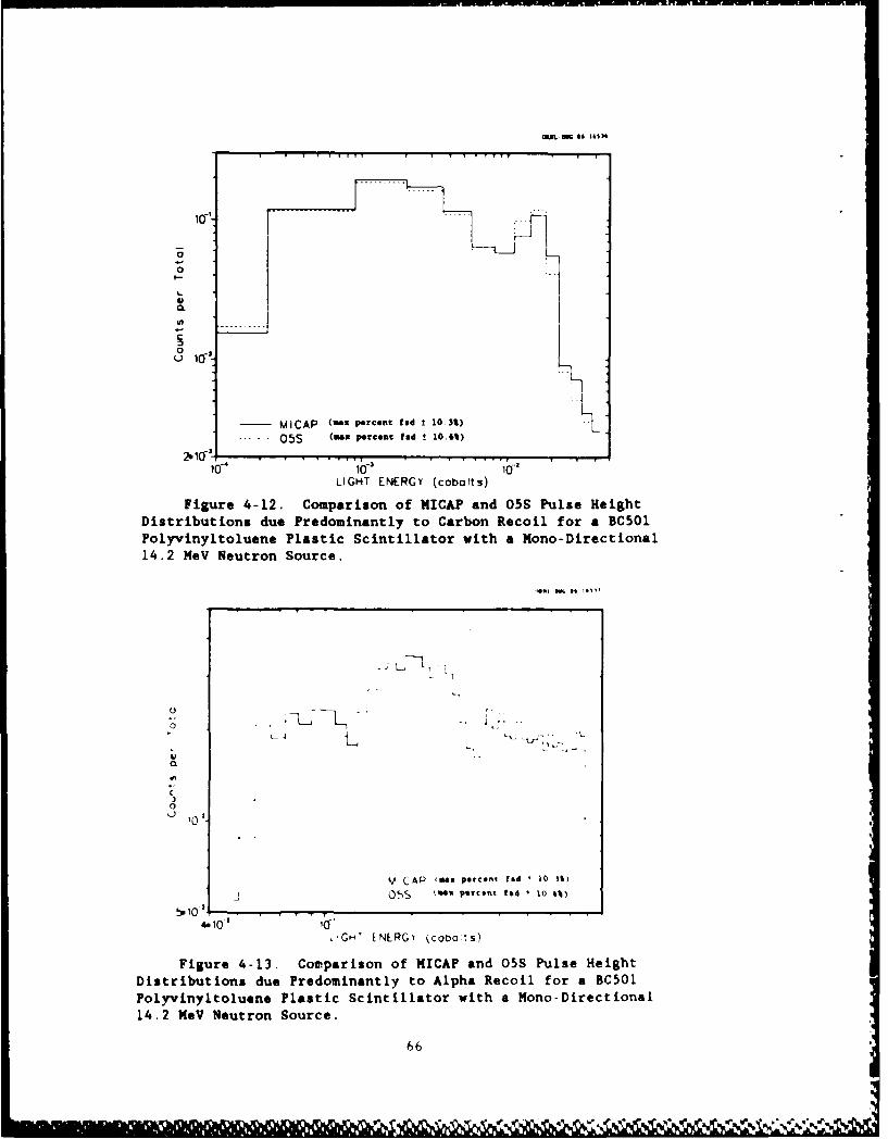
107'_- ------- -
0
4"
C
o 0
MIA UXpercent fed ± 10 3%)H
----05S (max percent fad t 10.1)
00-LI GHT ENERGYV (coboIt s)
Figure 4-12. Comparison of MICAP and 05S Pulse HeightDistributions due Predominantly to Carbon Recoil for a BCS01Polyvinyltoluene Plastic Scintillator vith a Mono-Directional14.2 MeV Neutron Source.
5e 10I.,
4*1 10
*,;H ENRG coL~
Fiue41.Cmarsno IA nd0SPleHih
Ditiuin u rdmnnl oApaRci o C0
PoyinytleePatcSitlao ihaMn-ie inl
142MVNuto ore
I6
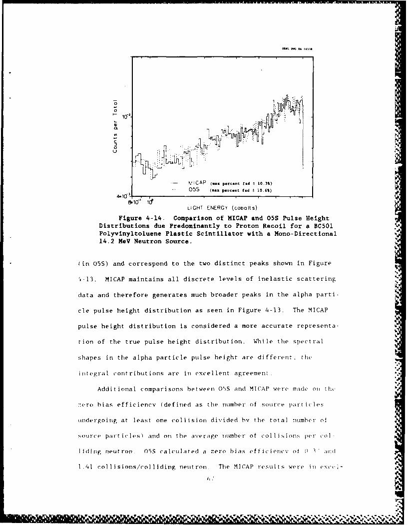
OL N DG 16 16 31
0
410- 1 -" I
0
vICAP (ma percent fsd ±10.3%)05S (max percent fed t 0.6%)
LIGHT ENERGY (cobolts)
Figure 4-14. Comparison of MICAP and 05S Pulse HeightDistributions due Predominantly to Proton Recoil for a BC501Polyvinyltoluene Plastic Scintillator with a Mono-Directional14.2 MeV Neutron Source.
(in 05S) and correspond to the two distinct peaks shown in Figure
L-13. MICAP maintains all discrete levels of inelastic scattering
data and therefore generates much broader peaks in the alpha parti-
cle pulse height distribution as seen in Figure 4-13. The MICAP
pulse height distribution is considered a more accurate representa-
tion of the true pulse height distribution. While the spectral
shapes in the alpha particle pulse height are different, the
integral contributions are in excellent agreement. '-
Additional comparisons between 05S and MICAP were made on tfl
.ero bias efficiencv (defined as the number of source part icles
undergoing at least one collision divided by the total number of
source part icles and on the average number of collisions per col-
I iding neutron. 05S calculated a zero bias ef ficiencv of 0 " and
1.41 collisions/colliding neutron. The MICAP results were in excel-
11 1 1 1 1 ,I1 . .
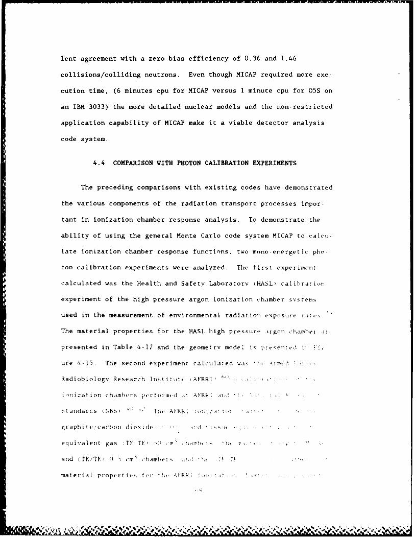
lent agreement with a zero bias efficiency of 0.36 and 1.46
collisions/colliding neutrons. Even though MICAP required more exe-
cution time, (6 minutes cpu for MICAP versus 1 minute cpu for 05S on
an IBM 3033) the more detailed nuclear models and the non-restricted
application capability of MICAP make it a viable detector analysis
code system.
4.4 COMPARISON WITH PHOTON CALIBRATION EXPERIMENTS
The preceding comparisons with existing codes have demonstrated
the various components of the radiation transport processes impor-
tant in ionization chamber response analysis. To demonstrate the
ability of using the general Monte Carlo code system MICAP to calcu-
late ionization chamber response functions, two mono-energetic pho-
ton calibration experiments were analyzed. The first experiment
calculated was the Health and Safety Laboratory IHASL) calibratioll
experiment of the high pressure argon ionization chamber systems
used in the measurement of environmental radiation exposure raes
The material properties for the HASL high pressure argon chambel i:,
presented in Table 4-12 and the geometry model is presend
ure 4-15. The second experiment calculated ai ,.-\:v ,
Radiobiologv Research Instiltute iAFRRI -,
ionizat ion chaiph irS perftorvntd i* AFRRI ,T;!
tandards NBS } *. Th AFRR: ::i . ' '
F'raphite:carbon dioxide A! i ,' * .
equivalent gas (TE T - ,' r hanh, r
and (TE TF) ) -) cm, 2hamhet , " -l
material propert ies tor ht. .\RR : r
P* N OF 'r ff % %
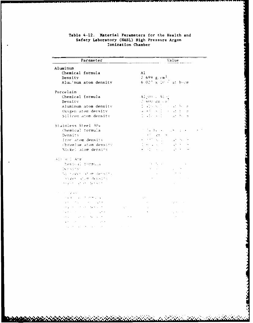
Table 4-12. Material Parameters for the Health and
Safety Laboratory (HASL) High Pressure Argon
Ionization Chamber
Parameter Value
AluminumChemical formula AlDensity 2 6QQ g. cm 3
AluL.fnum atom density 6.02> x C at bcTr
PorcelainChemical formula A, '0, Si
Dens itv .7 Jjr
Aluminum atom densiv.
Oxvgen atom dersitv - -: :
Sil icon atom density.
Stairless Steel 30-.Chemical formula , -
Dens it1I',T' rior densi, .
,'hromiun' atom densNicke atom densv -
t"
If-
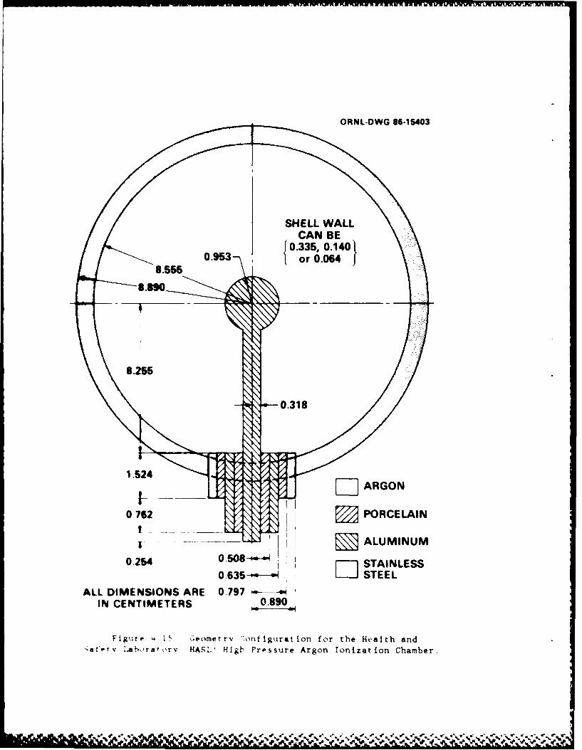
ORNL-DWG 86-15403
SHELL WALLCAN BE
0.335, 0.1400.953 or 0.064
0.254556 TILS
ALL DMENSINS AE 079RGON
IN CENTIMETERS 0.00890
Figure - 1 Ceometrv C7onfiguration for the Health and-&*@TV !Aborarorv HASI.) High Pressure Argon Ionization Chamber.
LM* * r ~* *~ % - * -
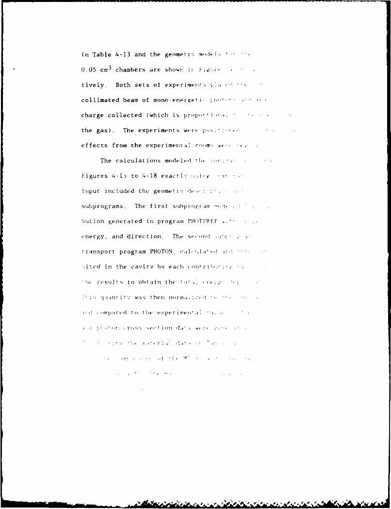
in Table 4-13 and the geometr ,.
0.05 cm3 chambers are showT ii
tively. Both sets of experimr- ,..
collimated beam of mono-energe i, , "
charge collected (which is prp,,r i
the gas). The experiments were p,"..
effects from the experimental , I
The calculations modeleId ,. :,,-
Figures 4-15 to 4-18 exactlyv ' ri, .. vr
input included the geomer 1v ,1#",, : 1;"
subprograms. The first sIabpog, .CTI ",4,.
)ut ion generated in program PH'TPP:'
energy, and direction. The sc.c,r~d -,."
transport program PHOTON, cal,, ila-l , -t
1 ited in the cavity bv each co t i i h,:'
* ii results to obtain the ;, ,, , : . .
i* I ,- ' L nt i "; wa s t hen no rn ,' . ,
, mpard to t he o:perime "
ros4 ()I ( , ' . .
Radl.hi.b1 av ;#evearh 'not It .1. AFVP
m* I a vr ah
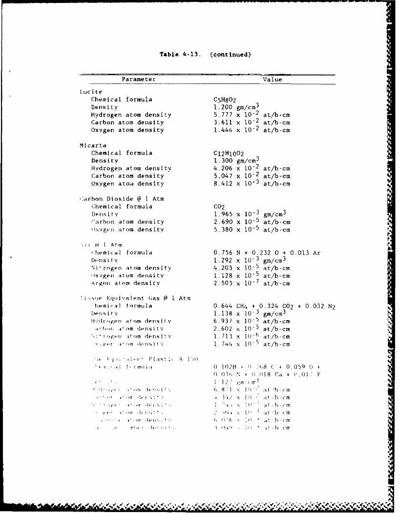
Table 4-13. (continued)
Parameter Value
Luc i teChemical formula C5H802Density 1.200 gm/cm 3
Hydrogen atom density 5.777 x 10⁻² at/b-cmCarbon atom density 3.611 x 10⁻² at/b-cmOxygen atom density 1.444 x 10⁻² at/b-cm
MicartaChemical formula C12HI002Density 1.300 gm/cm 3
Hydrogen atom density 4.206 x 10⁻² at/b-cmCarbon atom density 5.047 x 10⁻² at/b-cmOxygen atoai density 8.412 x 10 - 3 at/b-cm
Carbon Dioxide @ 1 Atm
Chemical formula C02Density 1.965 x 10- 3 gm/cm 3
Carbon atom density 2.690 x i0- 5 at/b-cm
,J:.vgen atom density 5.380 x 10- 5 at/b-cm
.lr (di I Atm
Clhemical formula 0.756 N + 0.232 0 + 0.013 ArDensitv 1.292 x 10⁻³ gm/cm 3
Nitrogen atom density 4.203 x 10- 5 at/b-cm,Uxvgen atom density 1.128 x 10 - 5 at/b-cm
Argon atom density 2.503 x 10- 7 at/b-cm
i. ,ife Equi'.'a Ient Gas @ 1 Atmhemical formula 0.644 CH4 + 0.324 C02 + 0.032 N2
Jns it'v 1.138 x I0 - gm/cm3
H'droe, n atom density 6.937 x 10- 5 at/b-cmA!-hwi .iom densitv 2.602 x 10- 5 at/b-cm
' I 'e, 1 ,t om densit 1. 713 x 10 . 6 at/b-cm*..K.r i 'TI ,I4.I i t; 1. 7L4 x I0 5 at/b-cm
'.- !' l' :'. ,, l P la ,;t i. A I M<
,: , ,.Tlrtil,, O 102H * I) '68 C + 0.0 59 00( N ).018 Ca + (00 ' F
at 1) c--
4 +Pf i t ' -- a t C MLI r• " . x 1 ;• t ,b <m
S r .It ' . I ] it c 'm
;+ *r , ' ( h ' ' ," • B), + . U + ,it C) - M
.. % ****. S. ** ** *I.. .*~%#%*.~%Wt *&/~~~%.* *.~*.~**~ I..'. .. 'l , -. *_.

ORNL-DWG U.1501
PLSTREN
IN~~O CETIETR
0.476
KI
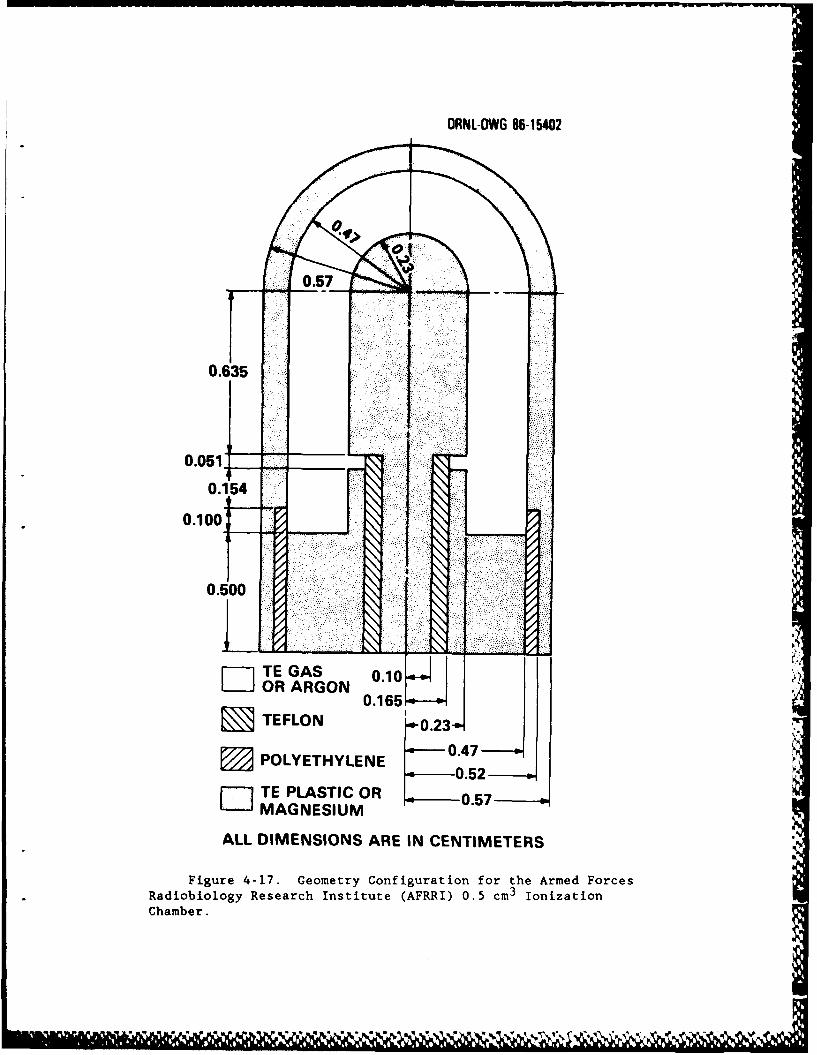
ORNL-DWG 86-15402
I057
0.835
0.05ji 1
0.154
0.100
0.500
m TE GAS 0.10io2LWOR ARGON0.6
STEFLON -e0.23--
~22POLYETHYLENE 0.527
f]TE PLASTIC OR 10 0.57LJ MAGNESIUM
ALL DIMENSIONS ARE IN CENTIMETERS
Figure 4-17. Geometry Configuration for the Armed ForcesRadiobiology Research Institute (AFRRI) 0.5 cm3 IonizationChamber.
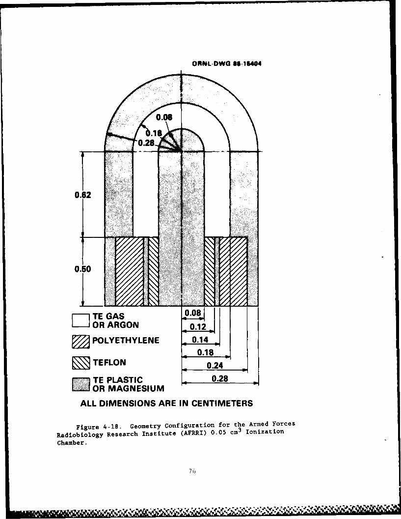
ORNL-DWG 3-64
0.62 0.08
0.50
D]OR ARGON0.
SPOLYETHYLENE 01
D TE PLASTIC 0.28OR MAGNESIUM
ALL DIMENSIONS ARE IN CENTIMETERS
Figure 4-18. Geometry configuration for the Armed Forces
Radiobiology Research Institute (AFRRI) 0.05 cm3 Ionization
Chamber.
76
MON, NI, 4. lq'l
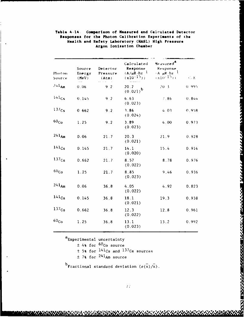
Table 4-14. Comparison of Measured and Calculated DetectorResponses for the Photon Calibration Experiments of the
Health and Safety Laboratory (HASL) High PressureArgon Ionization Chamber
Calculated Measureda
Source Detector Response ResponsePhot on Energy Pressure (A/AR-hr 1 (A MR-titSource (MeV) (Atm) (Xl0- 15) X I( 1)))_
24lm 0.06 9.2 20.2 b 20) 3 0 (W)(0.021)
141Cs 0.145 9.2 6.63 1.86 0.4(0.023)
13 7Cs 0 662 9.2 3.86 4.03 0.958(0.024)
60 CO 1.25 9.2 3.89 4.00 0.973(0.023)
241~m 0.06 21.7 20.3 21.9 0.928
(0.021)14 1Cs 0.145 21.7 14.1 15.4 0.916
(0.020)
13 7Cs 0.662 21.7 8.57 8.78 0.976(0.022)
6 0 CO 1.25 21.7 8.85 9.46 0.936(0.023)
241~m 0.06 36.8 4.05 4.92 0.823(0.022)
11s 0.145 36.8 18.1 19.3 0.938(0.021)
17S 0.662 36.8 12.3 12.8 0.961(0.022)
6 0CO 1.25 36.8 13.1 13.2 0.992(0.023)
aExperimental uncertainty
± 4% for 6 0Co source
± 5% for l4 lGs and 13 7Cs sources
± 7% for 2l source
Fcinl standard deviation (a(x)/x).
7,
huIt two casp, which involved low eiergv phot or) ,Io'r ,I* ' .xpl i
!,at ion could be tound as to why these two case% do tiot igl I , wt.
is t he other a ses The discrepancy for these two caises ( Id be
,,i tial Ilv due to al el'ro- in the expe-imelt (withinI the exi:;.l imeltilt
procedure itself or in the recording of the data) Furtheruntt-e, the
consistent underestimation of the experimental response by the MICAP'
calculations Is not understood at this time-
The comparisons of the MICAP and experimental results for the
AFRRI 50 cm3 ionization chambers are presented in Table 4-l'1 and th,.
comparisons of the MICAP and experimental results for the AFRRI 0.5
Cm 3 and 0.05 cm 3 ionization chambers are presented in Table 4-16.
The comparisons of calculated and experimental results for the 50
cm 3 ionization chambers show excellent agreement in Table 4-15. The
calculations analyzed 500,000 source particles incident on the
detector. The calculated-to-experimental ratios (C/E) are well
within 10% for all cases analyzed. The results also show a sys-
tematic overestimation for the C/CO 2 chamber and underestimation for
the TE/TE chamber. As in the HASL study, the exact cause is not
known. A sensitivity study was performed however, on the TE/TE and
C/CO 2 chambers with 0.72 cm wall thickness. Both chambers were
evaluated for a ±10% change in gas density and the C/CO 2 chamber was
evaluated for a ±5% change in graphite density. The effect of gas
density was significant in the sensitivity calculations. For the
TE/TE chamber, the C/E ratio was 0.902 for a -10% change in gas den-
sity and 1.08 for a +10% change. Likewise, for the C/CO 2 chamber,
the C/E ratio was 0.877 for a -10% change in gas density and 1.09
for a +10% change. Therefore, an error in the gas density
78
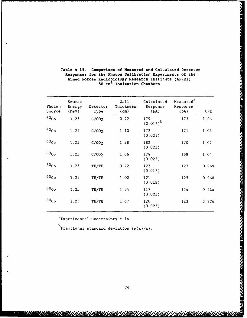
Table 4-15. Comparison of Measured and Calculated DetectorResponses for the Photon Calibration Experiments of theArmed Forces Radiobiology Research Institute (AFRRI)
50 cm3 Ionization Chambers
Source Wall Calculated Measured a
Photon Energy Detector Thickness Response ResponseSource (MeV) Type (cm) (pA) (pA) G/E6 0 Co 1.25 C/C02 0.72 179 b173 1.04
(0. 0 1 7 )b60 Co 1.25 C/C02 1.10 172 171 1.01
(0.021)6 0 Co 1.25 C/C02 1.38 182 170 1.07
(0.021)6 0Co 1.25 C/C02 1.66 174 168 1.04
(0.023)6 0Co 1.25 TE/TE 0.72 123 127 0.969
(0.017)6 0Co 1.25 TE/TE 1.02 121 125 0.968
(0.018)6 0CO 1.25 TE/TE 1.34 117 124 0.944
(0.023)6 0 Co 1.25 TE/TE 1.67 120 123 0.976
(0.023)
aExperimental uncertainty ± 1%.
bFractional standard deviation (a(x)/x).
79
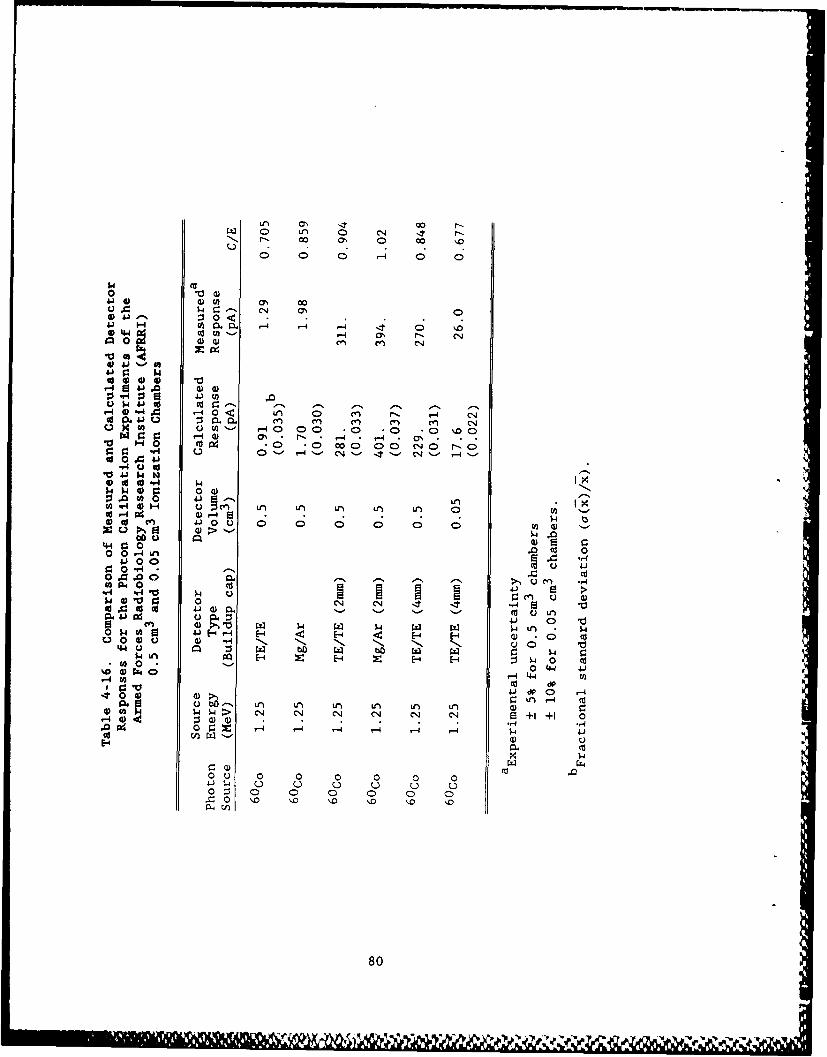
S 0 Lf) 01 c.iN - co 000
0> 0 C)- 0 0
4 r-s CN m' 04.1~ ~~~: H0 4 .4 .-4 - .
V44 cU)f.- a4 ON -f, cN
0 0. '.- a)0 n C
41 0
.4 4)-44 r-I0< Lfrl 0 CY) N. .- 4 C'.4
cMo (L'- 40 0 0 * 0 .0 .0 ' 0r. r r- 0) ON' r - * 4 . . M'. .H HO r Cd~ C*0 0 C'0 00C 1 0~ t- C
cd 0,4 4.1
w N0 0 0
(A "4 )H U cn1 LA Ln Ln Ln LA U0~ Cl 4-io" 0 0 0 0 0 0 C l 0 )-
44 r. .0 t 04 0 0 c o u 4
0 "4 -Cd
0 4 000 n r
co P4 0(d 14"4~~. 0o 4 0c ) 4$40- 4)- 00 a 1000 0 cc4 No N) N. No N Nad.4 :s4 41 0$4 (A4 4J -4 E-4 E-4 4) - 0 co
00. 0- 4C-4 41)
%0 f4) 40 r-4 4 4 I.- 4 M Cd dfI C:V" P0 r-4-t0 0 4 r ~Ln -4 cala 0cibo -SLA Ln V) Ln ULA LA 0)r
r4 4 :4 .4 C' a)- q) .,q .' C)q.0 ~ 0 . 4 - 4-4 r -4 .-4 w 41.
0ou 0 0 0 0 0 0', U U Q, U U0 Z 0 0 0 0 0 0
= . '. \0 '. '0 .
80
calculations will result in comparable errors in the calculated
results. The graphite wall density effects were found to be less
significant. The sensitivity study yielded a C/E ratio of 1.03 for
a -5% change in graphite density, and 0.99 for a +5% change. There-
fore, a slight error in graphite density will cause a lessor error
in the calculated response. For the problems analyzed, this error
was within the statistical error of the Monte Carlo calculations.
The results of the 0.5 cm3 and 0.05 cm3 calculations vary when
compared to experiment. As seen in Table 4-16, the C/E ratios range
from 0.677 to 1.02 for the different cases analyzed. Each chamber
was analyzed with 900,000 source particles incident on the chamber
wall material. Overall, the results indicate several trends in the
calculational ability of MICAP with respect to ionization chamber
size. First, MICAP appears to have difficulty reproducing the
smaller chamber results. This is evidenced by the 0.05 cm3 TE/TE
C/E ratio of 0.677 and the 0.5 cm3 TE/TE chamber (with no build-up
cap) C/E ratio of 0.705. Variations in wall thickness (nominally
0.1 cm) could partly be responsible for these discrepancies; how-z
ever, confirmation would require detailed sensitivity calculations.
A second trend is the larger C/E ratios for the smaller measured
signals. This could possibly be due to errors in the experimental
results. It should be noted that this same trend is apparent in the
experimental uncertainty presented at the bottom of Table 4-16.
One final result which contributes to the explanation of the
discrepancy between calculated and experimental results is seen in
the 6 0 Co pulse height distribution for the 50 cm3 TE/TE ionization
chamber shown in Figure 4-19. This curve is representative of the
81
*1' -
a
0
NICA? (max percent fad t 13.4%)
. .' V
ENERGY (e )
Figure 4-19. Pulse Height Distribution for the Armed Forces%
Radiobiology Research Institute (AFRRI) TE/TE 50 cm3
Ionization Chamber due to a Mono-Directional 60Co Photon Source.
pulse height distributions for the ionization chambers analyzed and
shows a broad distribution as a function of energy. Furthermore,
the pulse height contains a long high-energy tail which affects the
calculation of the average energy deposited per source particle.
Although the fractional standard deviation for the Monte Carlo
result in Table 4-15 was approximately ±2%, the tail of the pulse
height distribution could be undersampled and therefore lead to an
inaccurate calculated value.
The results of the photon calibration experiment comparisons
show the applicability of MICAP to ionization chamber response cal-
culations even though the AFRRI small chamber results were incon-
clusive. The ultimate and final evaluation of MICAP is made with
the mixed-field results presented in the next section.
82
J"I
4.5 COMPARISON WITH MIXED FIELD EXPERIMENTS
The results presented in the preceding sect ion dtmoi .v,,I "
ability of MICAP to calculate ionization chamber respoose fu*,: 1,:
for mono-energetic photon calibration experiments. Although :
verification is necessary, the real benefit of MICAP is for mitd
field experiments. To demonstrate the ability of using MI(AP :o
calculate ionization chamber response functions for mixed neutron
and photon radiation environments, three radiation experiments wert.
analyzed.4 2 -4 3 The first experiment analyzed was performed at the
NBS 2 52 Cf facility. This experiment involved exposing the 50 cm3
and 0.5 cm3 ionization chambers individually, in free air, at a nom-
252inal distance of 30 cm from the center of the Cf source. The
source and detector were positioned such that room effects were
negligible. The second and third experiments were performed at the
AFRRI TRIGA reactor described in Ref. 44. These experiments were
performed in exposure room 1 (ERI) of the reactor facility for two
of the most frequently used reactor configurations:
1. Bare room with no shielding placed between the experiment
and the reactor core (ER1 Free Field), and
2. 15 cm lead shield placed in front of the reactor tank wall
to attenuate photons (ERi 15 cm Pb).
The AFRRI experiments exposed a pair of ionization chambers about 10
cm apart and approximately 100 cm from the reactor core center. The
experimental setup for the bare room (ERl Free Field) is shown in
Figure 4-20 and for the 15 cm lead shield (ERl 15 cm Pb) in Figure
4-21. The two ionization chambers exposed were the 0.5 cm3 TE/TE
83
ORNL-DWG 86-45406
REACTOR
CORE CENTER
I I I10 CM--§H608.33 cmi
-- a *30.48cm THICK WOOD WALLS COVERED BY0.3175 cm Gd2O3 PAINTED MASONITE BOARDS
1-4 608.33 cm
Figure 4-20. Schematic Top View of the Armed ForcesRadiobiology Research Institute (AFRRI) Experimental Room One FreeField (ERi FF) Experiment.
63 979 KYELOPIET AMD EVAILUATION OF A MONTE CARLO CODE SYSlEN AiM- FOR AINA.YSIS OF IONIZATION CHAMBER RESPONSES(U) OAK
RIMGE NATIONAL LAB TN J 0 JOHNRON ET AL. JUL 8?WIOARSSIFIED OANL./T-±19E9 F/O 16/4 MI.
Lapm .. W
31.25
MlAYl v Rlc'i I ITOIN TEST CHART
o..
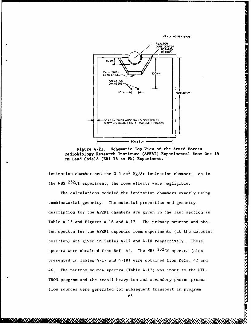
ORNL-DWG 86-45405
REACTORCORE CENTER
BORATEDBOARDS
30 cm j j\,/
15cm THICK I
LEAD SHIELD
IONIZATIONCHAMERS--,"
O cm-i 608 33 cm
_W 3.48 cm THICK WOOD WALLS COVERED BY0.3175 cm GdO 3 PAINTED MASONITE BOARDS
1608 33cm
Figure 4-21. Schematic Top View of the Armed ForcesRadiobiology Research Institute (AFRRI) Experimental Room One 15cm Lead Shield (ER1 15 cm Pb) Experiment.
ionization chamber and the 0.5 cm3 Mg/Ar ionization chamber. As in
the NBS 2 5 2Cf experiment, the room effects were negligible.
The calculations modeled the ionization chambers exactly using
combinatorial geometry. The material properties and geometry
description for the AFRRI chambers are given in the last section in
Table 4-13 and Figures 4-16 and 4-17. The primary neutron and pho-
ton spectra for the AFRRI exposure room experiments (at the detector
position) are given in Tables 4-17 and 4-18 respectively. These
spectra were obtained from Ref. 45. The NBS 2 5 2Cf spectra (also
presented in Tables 4-17 and 4-18) were obtained from Refs. 42 and
46. The neutron source spectra (Table 4-17) was input to the NEU-
TRON program and the recoil heavy ion and secondary photon produc-
tion sources were generated for subsequent transport in program
85
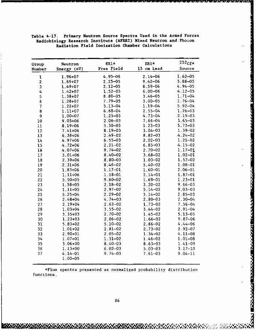
Table 4-17. Primary Neutron Source Spectra Used in the Armed ForcesRadiobiology Research Institute (AFRRI) Mixed Neutron and Phocon
Radiation Field Ionization Chamber Calculations
Group Neutron ERl* ERl* 252Cf*Number Energy (eV) Free Field 15 cm Lead Source
1 1.96+07 4.95-06 2.14-06 1.62-052 1.69+07 2.25-05 9.42-06 5.88-053 1.49+07 2.12-05 8.59-06 4.94-054 1.42+07 1.52-05 6.00-06 4.12-055 1.38+07 8.80-05 3.46-05 1.71-046 1.28+07 7.79-05 3.00-05 1.76-047 1.22+07 3.13-04 1.19-04 5.92-04
8 1.11+07 6.68-04 2.55-04 1.26-039 1.00+07 1.25-03 4.73-04 2.19-03
10 9.05+06 2.06-03 7.66-04 3.65-0311 8.19+06 3.30-03 1.23-03 5.73-0312 7.41+06 8.19-03 3.04-03 1.39-0213 6.38+06 2.49-02 8.82-03 4.24-0214 4.97+06 6.55-03 2.02-03 1.21-0215 4.72+06 2.21-02 6.85-03 4.15-0216 4.07+06 9.74-02 2.70-02 1.17-0117 3.01+06 8.40-02 3.68-02 1.02-0118 2.39+06 8.80-03 1.03-02 1.57-0219 2.31+06 8.46-02 5.40-02 1.08-0120 1.83+06 1.17-01 1.60-01 2.06-0121 1.11+06 1.18-01 2.14-01 1.87-0122 5.50+05 9.60-02 1.69-01 1.23-0123 1.58+05 2.18-02 3.20-02 9.66-0324 1.11+05 2.97-02 5.14-02 9.03-0325 5.25+04 2.29-02 3.14-02 2.85-0326 2.48+04 4.74-03 2.80-03 2.30-0427 2.19+04 2.62-02 1.73-02 7.56-0428 1.03+04 3.55-02 3.44-02 2.91-0429 3.35+03 2.70-02 1.45-02 5.13-0530 1.23+03 2.06-02 1.66-02 9.87-0631 5.83+02 5.10-02 2.86-02 4.44-0632 1.01+02 2.81-02 2.73-02 2.92-0733 2.90+01 2.05-02 1.34-02 4.11-0834 1.07+01 1.31-02 1.46-02 1.01-0835 3.06+00 8.40-03 8.63-03 1.41-0936 1.13+00 6.02-03 5.03-03 3.17-1037 4.14-01 9.74-03 7.61-03 9.04-11
1. 00-05
*Flux spectra presented as normalized probability distributionfunctions.
86
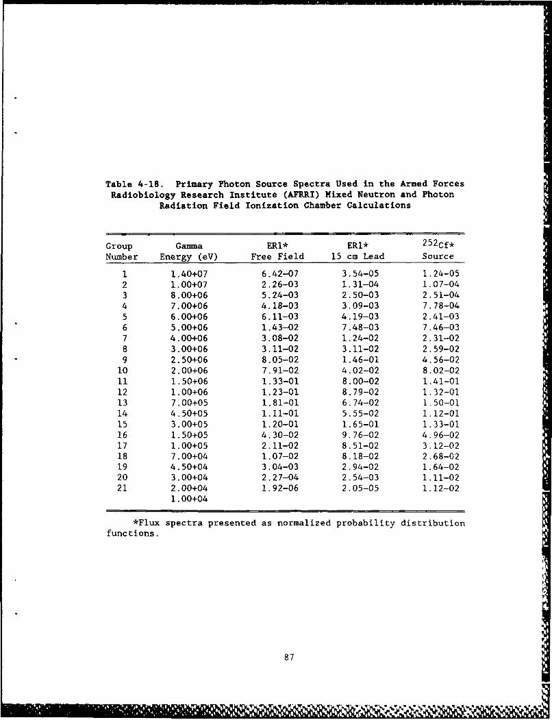
Table 4-18. Primary Photon Source Spectra Used in the Armed ForcesRadiobiology Research Institute (AFRRI) Mixed Neutron and Photon
Radiation Field Ionization Chamber Calculations
Group Gamma ER1* ERl* 2 5 2Cf*
Number Energy (eV) Free Field 15 cm Lead Source
1 1.40+07 6.42-07 3.54-05 1.24-052 1.00+07 2.26-03 1.31-04 1.07-043 8.00+06 5.24-03 2.50-03 2.51-044 7.00+06 4.18-03 3.09-03 7.78-045 6.00+06 6.11-03 4.19-03 2.41-036 5.00+06 1.43-02 7.48-03 7.46-037 4.00+06 3.08-02 1.24-02 2.31-028 3.00+06 3.11-02 3.11-02 2.59-029 2.50+06 8.05-02 1.46-01 4.56-02
10 2.00+06 7.91-02 4.02-02 8.02-0211 1.50+06 1.33-01 8.00-02 1.41-0112 1.00+06 1.23-01 8.79-02 1.32-0113 7.00+05 1.81-01 6.74-02 1.50-0114 4.50+05 1.11-01 5.55-02 1.12-0115 3.00+05 1.20-01 1.65-01 1.33-0116 1.50+05 4.30-02 9.76-02 4.96-0217 1.00+05 2.11-02 8.51-02 3.12-0218 7.00+04 1.07-02 8.18-02 2.68-0219 4.50+04 3.04-03 2.94-02 1.64-0220 3.00+04 2.27-04 2.54-03 1.11-0221 2.00+04 1.92-06 2.05-05 1.12-02
1.00+04
*Flux spectra presented as normalized probability distribution
functions.
87
HEAVY and program PHOTON, respectively. Because the detector effi-
ciency (with respect to neutron interactions) was so poor, a ficti-
tious scattering model was incorporated in the NEUTRON program to
facilitate interactions. This eliminated the capability of produc-
ing a pulse height distribution, and therefore one analog Monte
Carlo case was also performed. With the fictitious scattering
model, approximately 200,000 to 500,000 source particles were
analyzed to obtain a fractional standard deviation less than ±10.
These cases used approximately 15 to 35 minutes of cpu time on an
IBM 3033. The analog case modeled 3,000,000 source particles to
obtain the same fractional standard deviation and used approximately
3 hours and 20 minutes cpu time. As in the case with the photon
calibration experiments, the primary photon source spectra (Table
4-18) were modeled in program PHOTPREP to generate an input source
tape for program PHOTON. The PHOTON source tape modeled 900,000
photons incident on the ionization chamber wall. The results from
program HEAVY and program PHOTON were analyzed to obtain the total
energy deposited in the cavity by particle type i.e., protons, alpha
particles, primary photons, etc. These results were then normalized
to the incident source strength to obtain the neutron, photon and
total response of the ionization chamber. The cross sections and
material data for the transport programs were generated using the
neutron and photon cross section processor modules MICRO, MACRO, and
PECSP. Recombination effects were assumed negligible, and therefore
were not considered.
The comparisons of the calculated and experimental total ioni-
zation chamber responses to the mixed field experiments are
88
presented in Table 4-19. The calculated-to-experimental ratios
(C/E) show excellent agreement in all the cases except the 0.5 cm
Mg/Ar chamber in the ERI 15 cm Pb field. Like the mono-energetic
photon results, the largest discrepancy (excluding the case men-
tioned above) occurs for the smallest measured response. A portion
of this discrepancy could therefore be due to experimental error.
The Monte Carlo results have a fractional standard deviation less
than ±10% for all calculations. This fractional standard deviation
is for the detector response per incident source particle i.e.,
Amps/(n-cm2 -sec-kW) or Amps/(7-cm 2-sec-kW). To compare with the
measured response, an absolute normalization was obtained from the
spectra presented in Ref. 45 for the two AFRRI experiments. While
the spectral shapes in Ref. 45 are probably accurate to within ±10%,
the absolute normalization is known to within only ±15-20%, espe-
cially for the AFRRI ERI 15 cm Pb cases. Therefore, the MICAP cal-
culated results in Table 4-19 are within the statistical error of
the information used.
The AFRRI ERI 15 cm Pb calculation using the 0.5 cm3 Mg/Ar ion-
ization chamber displayed an interesting result in the neutron
response analysis. In viewing the geometry description in Figure
4-17, a thin polyethylene strip (approximately 0.1-cm-high) is shown
in contact with the gas region. The polyethylene acts as an insula-
tor between the outside wall and the central electrode. The
analysis of the results from program HEAVY shows recoil argon ions
from neutron interactions in the gas, and proton recoils from neu-
tron interactions with hydrogen in the polyethylene strip, as the
only two sources of energy deposition in the gas. Furthermore,
89
Jl v or
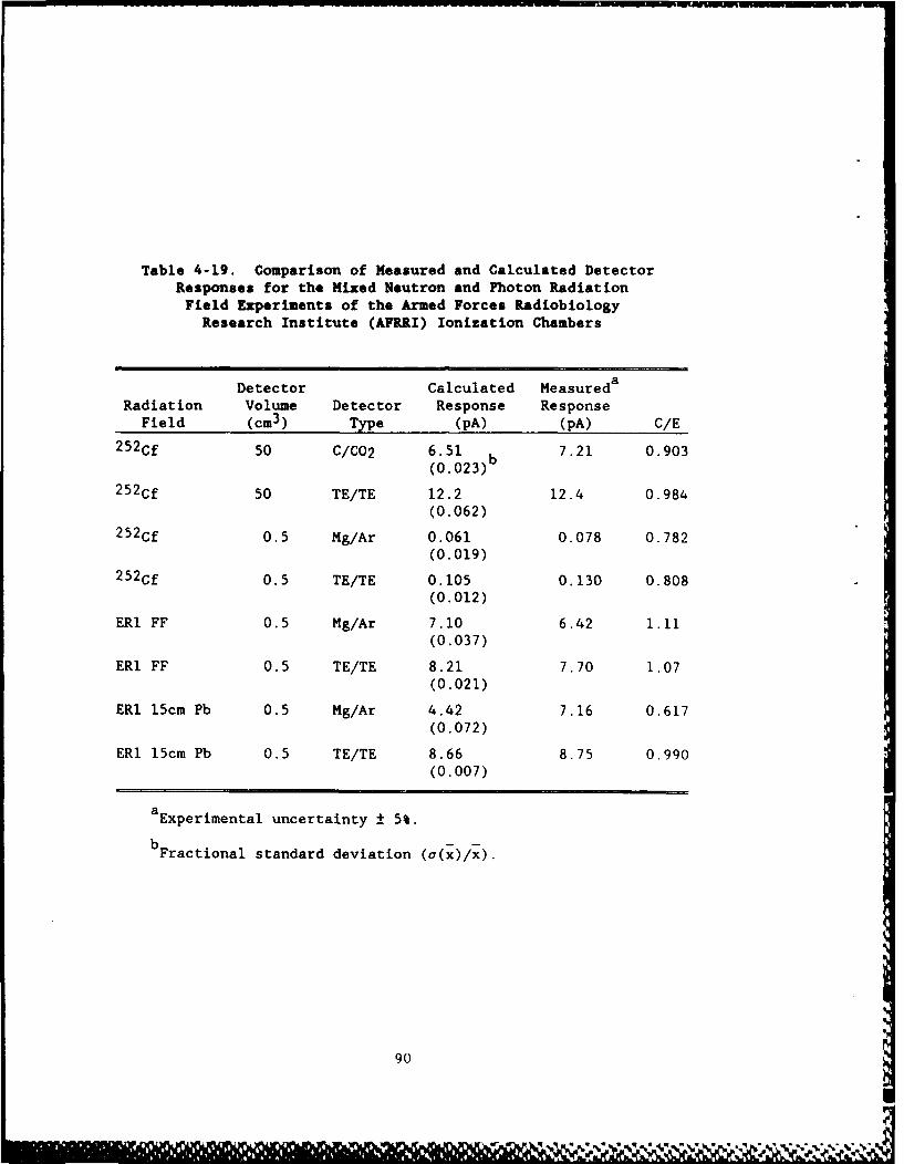
Table 4-19. Comparison of Measured and Calculated DetectorResponses for the Mixed Neutron and Photon RadiationField Experiments of the Armed Forces Radiobiology
Research Institute (AFRRI) Ionization Chambers
Detector Calculated Measureda
Radiation Volume Detector Response ResponseField (cm3) Type (pA) (pA) C/E
252Cf 50 C/C02 6.51 b 7.21 0.903
(0.023)252Cf 50 TE/TE 12.2 12.4 0.984
(0.062)2 5 2Cf 0.5 Mg/Ar 0.061 0.078 0.782
(0.019)252Cf 0.5 TE/TE 0.105 0.130 0.808
(0.012)
ERI FF 0.5 Mg/Ar 7.10 6.42 1.11(0.037)
ERI FF 0.5 TE/TE 8.21 7.70 1.07(0.021)
ERI 15cm Pb 0.5 Mg/Ar 4.42 7.16 0.617(0.072)
ERI 15cm Pb 0.5 TE/TE 8.66 8.75 0.990(0.007)
aExperimental uncertainty ± 5%.
bFractional standard deviation (a(x)/x).
90
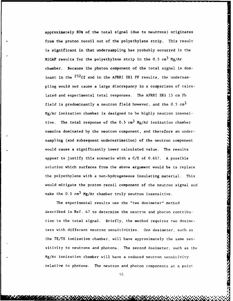
approximately 80% of the total signal (due to neutrons) originates
from the proton recoil out of the polyethylene strip. This result
is significant in that undersampling has probably occurred in the
MICAP results for the polyethylene strip in the 0.5 cm3 Mg/Ar
chamber. Because the photon component of the total signal is dom-
inant in the 2 5 2Cf and in the AFRRI ERI FF results, the undersam-
pling would not cause a large discrepancy in a comparison of calcu-
lated and experimental total responses. The AFRRI ERI 15 cm Pb
field is predominantly a neutron field however, and the 0.5 cm3
Mg/Ar ionization chamber is designed to be highly neutron insensi-
tive. The total response of the 0.5 cm3 Mg/Ar ionization chamber
remains dominated by the neutron component, and therefore an under-
sampling (and subsequent underestimation) of the neutron component
would cause a significantly lower calculated value. The results
appear to justify this scenario with a C/E of 0.617. A possible
solution which surfaces from the above argument would be to replace
the polyethylene with a non-hydrogeneous insulating material. This
would mitigate the proton recoil component of the neutron signal and
make the 0.5 cm3 Mg/Ar chamber truly neutron insensitive.
The experimental results use the "two dosimeter" method
described in Ref. 47 to determine the neutron and photon contribu-
tion to the total signal. Briefly, the method requires two dosime-
ters with different neutron sensitivities. One dosimeter, such as
the TE/TE ionization chamber, will have approximately the same sen-
sitivity to neutrons and photons. The second dosimeter, such as the
Mg/Ar ionization chamber will have a reduced neutron sensitivity
relative to photons. The neutron and photon components at a point
91
-i '
p " ' ' "
' ' ' V - 4"
in the radiation field can be computed from the response of the two
ionization chambers through the use of two simultaneous equations
and the detector responses to the photon calibration experiments.
MICAP on the other hand, requires only the analysis of the ioniza-
tion chamber with approximately equal neutron and photon sensitivi-
ties to ascertain the relative components of the total response. A
comparison of these results in Table 4-20 show excellent agreement
thus reaffirming the ability of MICAP to calculate mixed field radi-
ation experiments.
The final results presented for the mixed neutron and photon
radiation fields are the pulse height distributions for the 50 cm3
TE/TE ionization chamber in the 2 52Cf source field. As stated ear-
lier, only one analog Monte Carlo case was performed and therefore
only one set of pulse heights are possible. The pulse height dis-
tribution due to the 2 5 2Cf photon source presented in Figure 4-22 is
very similar to the 6 0 Co pulse height presented in Figure 4-19.
Therefore, the arguments presented with respect to the 6 0 Co pulse
height distribution are equally applicable here. The pulse height
distribution for the 2 5 2Cf neutron source presented in Figure 4-23
depicts a continuously decreasing curve as a function of increasing
energy. While there are significantly more contributions in the!
lower energy bins, these particles are outweighed by much larger
energy depositions of the fewer particles in the higher energy bins.
For the pulse height distribution shown in Figure 4-23, the average
energy deposited is approximately 3.0 x 10- 4 MeV/neutron. As in the
case with the photon pulse height distributions, undersampling of
the long high energy tail in the neutron pulse height distribution
92
p
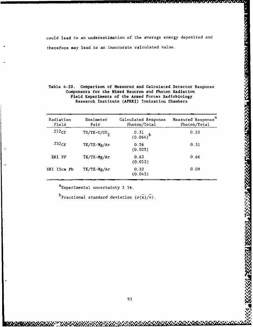
could lead to an underestimation of the average energy deposited and
therefore may lead to an inaccurate calculated value.
Table 4-20. Comparison of Measured and Calculated Detector ResponseComponents for the Mixed Neutron and Photon Radiation
Field Experiments of the Armed Forces RadiobiologyResearch Institute (AFRRI) Ionization Chambers
Radiation Dosimeter Calculated Response Measured Responsea
Field Pair Photon/Total Photon/Total2 52Cf TE/TE-C/CO 2 0.31 0.33
(0 .064 )b
252Cf TE/TE-Mg/Ar 0.26 0.31
(0.025)
ERI FF TE/TE-Mg/Ar 0.63 0.66(0.012)
ERI 15cm Pb TE/TE-Mg/Ar 0.10 0.09(0.043)
aExperimental uncertainty ± 5%.
Fractional standard deviation (a(x)/x).
93-
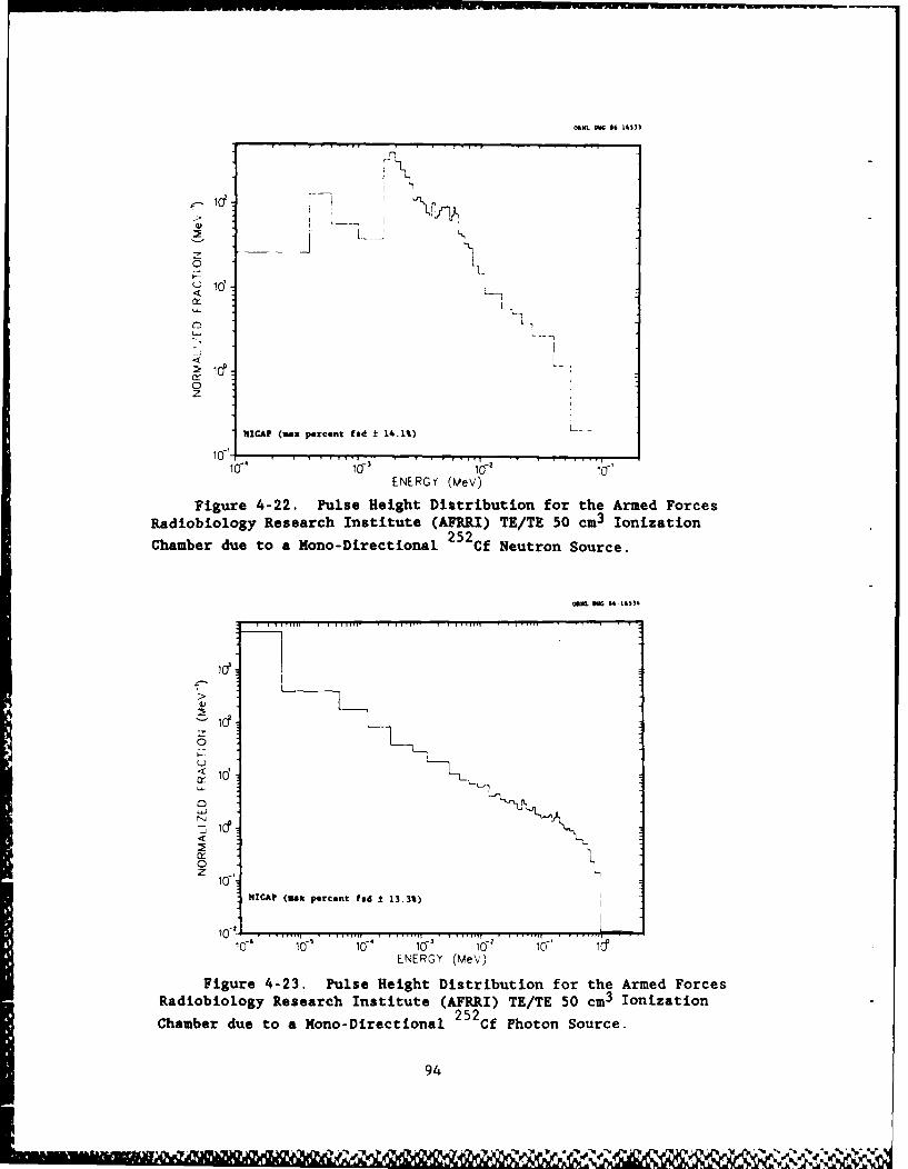
oOL WdG 86 153)3
LI
0
i -
0
HICA? (ias percenit fad ±14.1%)
ENERGY (MeV)
Figure 4-22. Pulse Height Distribution for the Armed ForcesRadiobiology Research Institute (A MRI) TE/TE 50 cm3 Ionization
Chamber due to a Mono-Directional 22Cf Neutron Source.
OSUL WIG $6 1651
>
0
I-;
S10' ,
0
ENERGY (MeV)
Figure 4-23. Pulse Height Distribution for the Armed ForcesRadiobiology Research Institute (AFRRI) TE/TE 50 cm3 Ionization
Chamber due to a Mono-Directional 252 Cf Photron Source.
49
10N
> IA mwpretfd±1.%
-2- ] _
ENRY_ MVFiue42. PleHih itiuinfrteAmdFre
Raioboog-esachIsttte(F___E/E50. 3 oizto< 252
Chabe duoaMn-Drcinl C. Pooore
= 94
CHAPTER V
CONCLUSIONS
This research project has consisted of the development and
verification of a new Monte Carlo code system for calculating
ionization chamber responses to mixed neutron and photon radiation
environments. This new code system, MICAP - Monte Carlo Ionization
Chamber Analysis Package, represents a unique capability in the area
of ionization chamber response analysis for mixed field dosimetry.
A five part verification program was used to examine all aspects of
the radiation processes applicable to ionization chamber analysis.
The verification program involved comparisons with results obtained
from existing codes as well as comparisons to experimental data.
The comparisons with existing codes verified the individual
aspects of MICAP with respect to ionization chamber analysis. More
specifically, iron transmission comparisons with MORSE yielded
excellent agreement (within the Monte Carlo statistical error) in
the neut:on leakage spectra, secondary photon production spectra,
and the photon leakage spectra for various neutron sources and iron
slab thicknesses. Secondly, comparisons with MACK-IV and RECOIL
data verified the nuclear models used in MICAP to describe the
individual nuclear reactions with an agreement to within 10% for
average energy depositions and kerma factors. Finally, the
comparison to 05S, a specialized Monte Carlo detector analysis cod,-
which has been used extensively, showed excellenzt agreement irn tht
pulse height distributions for a plastic scintillator, azid
therefore, verified the charged particle transport pro'es~s.
95
The comparisons with experimental data first evaluated MICAP
with respect to photon calibration experiments. The results from
these comparisons yielded agreement generally to within 10% for the
ionization chamber responses to the mono-energetic photon sources.
Finally, the comparisons with experiments performed in the mixed
neutron and photon radiation environments at NBS and AFRRI verified
the applicability of MICAP to mixed field ionization chamber
response analysis. The calculated results agreed with experimental
results to within the statistical error of the Monte Carlo and the
normalization of the experimental data.
The final product (MICAP) represents a valuable tool to
radiation dosimetry. The modular code system provides the most
rigorous treatment to date of the particle transport processes
applicable to ionization chamber response analysis. The general
implementation procedures incorporated into MICAP allow the system
to be useful for many applications in the field of radiation
dosimetry. It is recommended that the code system be tested further
by additional comparisons with mixed field radiation experiments to
resolve the discrepancies noted in this document. Additional
recommendations for future work are presented in the next chapter.
96
N*.
CHAPTER VI
RECOMMENDATIONS FOR FUTURE WORK
This study has demonstrated the applicability of using a gen-
eral Monte Carlo code system for calculating an ionization chamber
response to a mixed neutron and photon radiation environment. The
FORTRAN code system developed and tested in this study is only a
prototype, not a production code. The current version of MICAP
could be improved along several lines within the present scope of
ionization chamber response calculations. In particular, the fol-
lowing modifications and/or investigations of MICAP are suggested:
I. Improving the programming through the use of more effi-
cient algorithms, ASSEMBLER language coding of the most
cpu-intensive subroutines, and modifying program input to
establish a more user friendly code system.
2. Incorporating more sophisticated and detailed charged par-
ticle evaporation models for the neutron induced charged
particle production reactions i.e., (n,p), (n,a), etc.
The more sophisticated models should yield a better
representation of the energy of the charged particles pro-
duced via neutron interactions.
3. Performing more comparisons with mixed neutron and photon
radiation experiments - especially experiments involving
high energy neutron sources to test the accuracy of the
97
9 V V
charged particle evaporation models and fuither substan-
tiate the applicability of MICAP to ionization chamber
response analysis.
4. Study the incorporation of a multiple scattering capabil-
ity in the low energy charged particle transport program
using theoretical and empirical formulas. The current
work contains only continuous energy loss models. Allow-
ing multiple scattering in the low energy charged particle
transport will yield a more accurate representation of the
physics.
5. Incorporating the fictitious scattering model used in the
present work as an input option to facilitate calculations
involving ionization chambers which exhibit low neutron
efficiency.
6. Completing the programming for the Monte Carlo source
biasing to improve the calculation statistics.
Finally, MICAP could be further generalized to operate as a point
Monte Carlo code system applicable to reactor core and reactor
shielding calculations. This could be accomplished through program
switches which engage (or dissengage) the portions of the code sys-
tem applicable to a particular problem. Such a code system would
truly represent a general Monte Carlo program applicable to all
aspects of radiation transport/dosimetry analysis.
98
MS&NI&
LIST OF REFERENCES
I M I j
LIST OF REFERENCES
1. H. W. Fulbright, "Ionization Chambers," Nuclear Instruments andMethods, Vol 162, Nos. 1-3, Part 1, pp. 21-28, 1979.
2. T. E. Burlin, "Cavity Chamber Theory," Radiation Dosimetry,Vol. 1, F. H. Attix, W. C. Roesch, and E. Tochlin, Eds.,Academic Press, New York, 1968.
3. Radiation Dosimetry: X Rays and Gamma Rays with Maximum PhotonEnergies Between 0.6 and 50 MeV, ICRU Report 14, InternationalCommittee on Radiation Units and Measurements, Washington,D.C., 1969.
4. Radiation Dosimetry: X Rays Generated at Potentials of 5 to150 keV, ICRU Report 17, International Committee on RadiationUnits and Measurements, Washington, D.C., 1970.
5. Measurement of Absorbed Dose in a Phantom Irradiated by a Sin-gle Beam of X or Gamma Rays, ICRU Report 23, International Com-mittee on Radiation Units and Measurements, Washington, D.C.,1973.
6. H. Schraube, "Concluding Discussion on Ion Chambers for NeutronDosimetry," Ion Chambers for Neutron Dosimetry, J. J. Broerse,Ed., EUR 6782, Commission of the European Community, Luxem-bourg, pp. 345-350, 1980.
7. An International Neutron Dosimetry Intercomparison (INDI), ICRUReport 27, International Committee on Radiation Units and Meas-urements, Washington, D.C., 1978.
8. J. J. Broerse, G. Burger, and M. Coppola, A European NeutronDosimetry Intercomparison Project (ENDIP), EUR 6004, Commissionof the European Community, Luxembourg, 1978.
9. H. Bichsel, J. Eenmaa, K. Weaver, and P. Wooten, "Dosimetry ofMixed Radiation Fields," proceedings of a Symposium on Biologi-cal Dosimetry, IAEA-SM-193/78, pp. 3-17, Int. Atomic EnergyAgency, Vienna, 1975.
10. Neutron Dosimetry for Biology and Medicine, ICRU Report 26,International Committee on Radiation Units and Measurements,Washington, D.C., 1977.
11. H. Ing et al., Compendium of Neutron Spectra in CriticalityAccident Dosimetry, IAEA-180, Int. Atomic Energy Agency,Vienna, 1978.
100
12. J. E. Turner et al., User's Manual for PHOEL-2, A Monte CarloComputer Code for Calculating Energies of Photoelectrons andCompton Electrons in Water, ORNL/TM-6954, Union Carbide Corp.Nuclear Div., Oak Ridge Natl. Lab., 1979.
13. J. E. Turner et al., "Calculated Electron Slowing Down Spectrafor Liquid Water Irradiated by X and Gamma Rays-Implicationsfor Photon RBE," Sixth Symposium on Microdosimetry, J. Booz andH. G. Ebert, Eds., Harwood Academic Publishers, London, 1978.
14. S. Pszona and M. Makarewicz, "Effect of Cavity Size on the Sen-sitivity of a TE-Walled, TE-Gas-Filled Ionization Chamber forFast Neutrons," Physics in Medicine and Biology, Vol. 27, No.8, pp. 1015-1022, 1982.
15. M. W. Waddell, Jr., User's Guide to PXMORSE, ORNL/CSD/TM-129,Union Carbide Corp. Nuclear Dii., Oak Ridge Natl. Lab., 1980.
16. M. W. Waddell, Jr., "A Continuous Energy Monte Carlo Code,"M.S. thesis, The University of Tennessee, Knoxville, 1980.
17. M. B. Emmett, The MORSE Monte Carlo Radiation Transport CodeSystem, ORNL-4972, Union Carbide Corp. Nuclear Div., Oak RidgeNatl. Lab., 1975.
18. T. A. Gabriel, J. D. Amburgey, and B. L. Bishop, CALOR-A MonteCarlo Program Package for the Design and Analysis of Calorime-ter Systems, ORNL/TM-5619, Union Carbide Corp. Nuclear Div.,Oak Ridge Natl. Lab., 1977.
19. R. L. Ford and W. R. Nelson, The EGS Code System: ComputerProgram for the Monte Carlo Simulation of Electromagnetic Cas-cade Showers, SLAC-210, Stanford Linear Accelerator Center,1978.
20. Average Energy Required to Produce an Ion Pair, ICRU Report 31,International Committee on Radiation Units and Measurements,Washington, D.C., 1979.
21. J. B. Birks, The Theory and Practice of Scintillation Counting,The Macmillian Company, New York, 1964.
22. Los Alamos Radiation Transport Group X-6, MCNP-A GeneralizedMonte Carlo Code for Neutron and Photon Transport, LA-7396-M,Los Alamos Natl. Lab., revised April 1981.
23. J. C. Nimal et al., Programme de Monte Carlo Polycinetique aTrois Dimensions, TRIPOLI-2, C.E.A., Saclay, 1980.
24. S. N. Cramer et al., The Use of Kernels in Studying NeutronTransport Problems, ORNL-TM-2508, Union Carbide Corp. NuclearDiv., Oak Ridge Natl. Lab., 1969.
101
. . .. ...... 9
25. D. E. Bartine et al., Low-Energy Electron Transport by theMethod of Discrete Ordinates, ORNL-TH-3438, Union Carbide Corp.Nuclear Div., Oak Ridge Natl. Lab., 1971.
26. R. Kinsey, ENDF-102 Data Formats and Procedures for theEvaluated Nuclear Data File, ENDF/B-V, BNL-NCS-50496,Brookhaven Natl. Lab., 1979.
27. L. L. Carter and E. D. Cashwell, Particle Transport Simulationwith the Monte Carlo Method, TID-26607, USERDA Technical Infor-mation Center, 1975.
28. D. G. Doran and N. J. Graves, Displacement Cross Sections andPKA Spectra: Tables and Applications, HEDL-TME 76-70, HanfordNatl. Lab., 1976.
29. L. Dresner, EVAP-A FORTRAN Program for Calculating the Evapora-tion of Various Particles from Excited Compound Nuclei, ORNL-TM-196, Union Carbide Corp. Nuclear Div., Oak Ridge Natl. Lab.,1961.
30. P. N. Stevens and H. C. Claiborne, Weapons Radiation ShieldingHandbook, DASA-1982-5, Defense Atomic Support Agency, Washing-ton, D.C., 1970.
31. N. M. Schaeffer, Reactor Shielding for Nuclear Engineers, TID-25951, USERDA Technical Information Center, 1973.
32. T. W. Armstrong and K. C. Chandler, SPAR A FORTRAN Program forComputing Stopping Powers and Ranges for Muons, Charged Pions,Protons, and Heavy Ions, ORNL-4869, Union Carbide Corp. NuclearDiv., Oak Ridge Natl. Lab., 1973.
33. J. 0. Johnson and T. A. Gabriel, A User's Guide to MICAP - AMonte Carlo Ionization Chamber Analysis Package, ORNL/TM-10340,Martin Marietta Energy Systems, Inc., Oak Ridge Natl. Lab., (tobe published in 1987).
34. M. A. Abdou, Y. Gohar, and R. Q. Wright, MACK-IV, A New Versionof MACK: A Program to Calculate Nuclear Response Functions forData in ENDF/B Format, ANL/FPP/TM-77-5, Argonne Natl. Lab.,1978.
35. T. A. Gabriel, J. D. Amburgey, and N. M. Greene, Radiation-Damage Calculations: Primary Recoil Spectra, DisplacementRates, and Gas-Production Rates, ORNL/TM-5160, Union CarbideCorp. Nuclear Div., Oak Ridge Natl. Lab., 1976.
36. R. E. Textor and V. V. Verbinski, 05S: A Monte Carlo Code forCalculating Pulse Height Distributions Due to MonoenergeticNeutrons Incident on Organic Scintillators, ORNL-4160, UnionCarbide Corp. Nuclear Div., Oak Ridge Natl. Lab., 1968.
102
37. S. N. Cramer and R. W. Roussin, Monte Carlo Analysis of a
Time-Dependent Neutron and Secondary Gamma Ray Integral Experi-ment on a Thick Concrete and Steel Shield, ORNL/TM-7972, UnionCarbide Corp. Nuclear Div., Oak Ridge Natl. Lab., 1981.
38. D. E. Bartine et al., 37 Neutron, 21 Gamma Ray Coupled, P3,Multigroup Library in ANISN Format, DLC-31/(DPL-l/FEWG), 1975.
39. J. A. DeCampo, H. L. Beck, and P. D. Raft, High Pressure ArgonIonization Chamber Systems for the Measurement of EnvironmentalRadiation Exposure Rates, HASL-260, Health and Safety Labora-tory, New York, 1972.
40. 1 Lt. M. A. Dooley, Armed Forces Radiobiological ResearchInstitute, letter to J. 0. Johnson, Oak Ridge Natl. Lab., OakRidge, Tennessee, dated May 18 1984.
41. 1 Lt. M. A. Dooley et al., "Wall Attenuation and ScatterCharacteristics of Ionization Chambers at the Armed ForcesRadiobiology Research Institute," draft report, Armed ForcesRadiobiology Research Institute, Bethesda, Maryland, 1986.
42. D. E. Eagleson, Armed Forces Radiobiology Research Institute(AFRRI), Bethesda, Maryland, private communications to J. 0.Johnson, Oak Ridge Natl. Lab., Oak Ridge, Tennessee, May-July1986.
43. 1 Lt. M. A. Dooley et al., "NBS-AFRRI Ionization Chamber Inter-comparison in Mixed Neutron and Gamma-Ray Radiation Fields,"TR-86-3, Armed Forces Radiobiology Research Institute, 1986.
44. J. A. Sholtis, Jr. and M. L. Moore, Reactor Facility, ArmedForces Radiobiology Research Institute, AFRRI TR 81-2, ArmedForces Radiobiology Research Institute, Bethesda, Maryland,1981.
45. V. V. Verbinski and C. G. Cassapakis, Calculation of the Neu-tron and Gamma-Ray Environment In and Around the AFRRI TRIGAReactor, DNA 5793F-2, Defense Nuclear Agency, Washington, D.C.,1981.
46. C. M. Eisenhauer, National Bureau of Standards, Washington, D.C., private communication to J. 0. Johnson, Oak Ridge Natl.Lab., Oak Ridge, Tennessee, July 1986.
47. American Association of Physicists in Medicine, "Protocol forNeutron Beam Dosimetry," AAPM Report No. 7 of Task Group 18,Fast Neutron Beam Physics, Radiation Therapy Committee, 1980.
103
ft. ft 3
ORNL/TM- 10196
INTERNAL DISTRIBUTION
1. F. S. Alsmiller 32. R. T. Santoro2. R. G. Alsmiller, Jr. 33. M. S. Smith3. D. E. Bartine 34. J. S. Tang4. B. L. Bishop 35. M. W. Waddell5. T. J. Burns 36. R. C. Ward6. D. G. Cacuci 37. R. M. Westfall7. D. H. Cook 38. A. Zucker8. S. N. Cramer 39. P. W. Dickson, Jr.9. J. K. Dickens (Consultant)
10. J. D. Drischler 40. G. H. Golub11. M. B. Emmett (Consultant)12. W. W. Engle, Jr. 41. R. Haralick
13-17. T. A. Gabriel (Consultant)18. D. T. Ingersoll 42. D. Steiner
19-23. J. 0. Johnson (Consultant)24. R. A. Lillie 43. Central Research Library25. F. C. Maienschein 44-48. EPMD Reports Office26. J. V. Pace III 49. ORNL Y-12 Technical Library27. R. W. Peelle Document Reference Section28. F. G. Perey 50-51. Laboratory Records29. L. M. Petrie 52. ORNL Patent Office30. R. W. Roussin31. J. C. Ryman
EXTERNAL DISTRIBUTION
53. Dr. Charles Aeby, Air Force Weapons Laboratory, Kirkland Air ForceBase, Albuquerque, NM 87117.
54. Office of Assistant Manager for Energy Research & Development,DOE-ORO, Oak Ridge, TN 37830.
55. Argonne National Laboratory, Library Services Department, 302-CE125,9700 S. Cass Avenue, Argonne, IL 60439.
56. T. W. Armstrong, Science Applications, Inc., P.O. Box 2807, La Jolla,CA 92038.
57. Miguel Awschalom, National Accelerator Laboratory, P. 0. Box 500,Batavia, IL 60510.
58. D. Berley, National Science Foundation, Washington, D.C. 20550.
10 C
59. Larry W. Brackenbush, Battelle PNL, P.O. Box 999, Richland, WA99352.
60. Dr. J. E. Brau, Dept. of Physics, University of Tennessee, KnoxvilleTN 37916.
61. Brookhaven National Laboratory, Attention: Research Library, Upton,NY 11973.
62. Dr. Bruce Brown, Fermi National Accelerator Laboratory, P. 0. Box500, Batavia, IL 60510.
63. Dr. David 0. Caldwell, Department of Physics, University ofCalifornia at Santa Barbara, Santa Barbara, CA 93106.
64. Dr. Ernest Coleman, Office of High Energy Physics, U.S. Department ofEnergy, MS ER-221, Washington, D.C. 20545.
65. Stanley B. Curtis, Lawrence Radiation Laboratory, Bldg. 29, Room 213,Berkeley, CA 94720.
66. Anna Di Cicacco, Exp. VAl, CERN, CHl211, Geneva, Switzerland.
67. Herbert Destaebler, Stanford Linear Accelerator Center, StanfordUniversity, Stanford, CA 94305.
68. Robert T. Devine, Defense Nuclear Agency, CDR, USN, Washington D.C.20305-1000.
69. Dr. G. Dietze, Physikalisch-Technische, Bundesallee 100, D-3300Braunschweig, WESTERN GERMANY.
70. R. D. Edge, Physics Department, University of South Carolina,Columbia, SC 29208.
71. C. M. Eisenhauer, National Bureau of Standards, Bldg. 245,Gaithersburg, MD 20899.
72. Dr. R. Eisenstein, Department of Physics, University of Illinois,Urbana, IL 61801.
73. Doug E. Engleson, Defense Nuclear Agency, Armed Forces RadiobiologyResearch Institute, Bethesda MD 20814.
74. Lt. Richard Engstrom, Air Force Weapons Laboratory, Kirkland AirForce Base, Albuquerque, NM 87117.
75. Dr. Chris Fabjan, CERN, Geneva 23, Switzerland.
76. Dr. G. Feldman, Stanford Linear Accelerator Center, StanfordUniversity, Stanford, CA 94305.
77. K. Goebel, Health Physics Group, CERN, 1211 Geneva 23, Switzerland.
106
78. Dr. D. Hitlin, Stanford Linear Accelerator Center, StanfordUniversity, Stanford, CA 94305.
79. Craig Jensen, Dept. of Nuclear Engineering, University of Oklahoma,Norman OK 73019.
80. Mr. Terrence Jensen, Dept. of Physics and Astronomy, The Universityof Rochester, Rochester, NY 14627.
81. Prof. D. Lal, Tata Institute of Fundamental Research, National Centreof the Government of India for Nuclear Science & Mathematics, HomiBhabha Rd., Bombay 5, India.
82. Lawrence Livermore Laboratory, Technical Information Department, P.O.Box 808, Livermore, CA 94550.
83. Library for Nuclear Science, Massachusetts Institute of Technology atMiddleton, Middleton, MA 01949.
84. Dr. V. S. Narasimham, Tata Institute of Fundamental Research, Bombay400 005, India.
85. W. R. Nelson, Stanford Linear Accelerator Center, StanfordUniversity, P. 0. Box 4349, Stanford, CA 94305.
86. Keran O'Brien, Health and Safety Laboratory, U.S. Department ofEnergy, 376 Hudson Street, New York, NY 10014.
87. Dr. T. R. Palfrey, Jr., Department of Physics, Purdue University,West Lafayette, IN 47907.
88. Dr. Robert Palmer, Brookhaven National Laboratory, Upton, NY 11973.
89. Dr. C. W. Peck, Department of Physics, California Institute ofTechnology, Pasadena, CA 91109.
90. Dr. R. E. Pevey, Savannah River National Laboratory, Aiken SC 29808.
91. Dr. David W. 0. Rogers, Head, Ionizing Radiation Standards, Divisionof Physics, National Research Council of Canada, Ottawa, Canada KIAOR6.
92. Dr. C. Rubbia, Lyman Laboratory, Harvard University, Cambridge, MA02138.
93. Dr. W. Schmidt, Institute of Experimental Nuclear Physics, Universityof Karlsruhe, 75 Karlsruhe, W. Germany.
94. The Secretary, Radiation Group, Lab II, CERN, 1211 Geneva 23,Switzerland.
95. Dr. Walter Selove, University of Pennsylvania, Department of Physics,Philadelphia, PA 19104.
107
96. B. S. P. Shen, Department of Astronomy, University of Pennsylvania,Philadelphia, PA 19104.
97. Stanford Linear Accelerator Center, Attention: Library, P. 0. Box4349, Stanford, CA 94305.
98. Dr. Alan Stevens, Accelerator Dept. Bldg. 911, Brookhaven NationalLaboratory, Upton, NY 11973.
99. G. R. Stevenson, Radiation Protection Group, Lab II, CERN, 1211Geneva 23, Switzerland.
100. Dr. L. Sulak, Department of Physics, University of Michigan, AnnArbor, MI 48109.
101. R. Tesch, DESY, Hamburg, Notkesteig 1, W. Germany.
102. Ralph H. Thomas, Lawrence Berkeley Laboratory, Occupational HealthOffice, 50A-5106, Engineering Division, Berkeley, CA 94720.
103. Dr. W. J. Willis, CERN, Geneva 23, Switzerland.
104. Dr. S. Yellin, Stanford University, Stanford Linear AcceleratorCenter, P. 0. Box 4349, Stanford, CA 94305.
105. G. B. Yodh, University of Maryland, College Park, MD 20742.
106. Robert Young, Director, Defense Nuclear Agency, ATTN: STRP, 6801Telegraph Road, Alexandria, VA 22310.
107. Dr. B. Zeitnitz, Nuclear Research Center, Karlsruhe, W. Germany93120.
108. Gary H. Zeman, Defense Nuclear Agency, CDR, MSC, USN, Armed ForcesRadiobiology Research Institute, Bethesda MD 20814.
109-343. Defense Nuclear Agency Transport Distribution (AU).
344-373. Technical Information Center, Oak Ridge Turnpike, Oak Ridge TN37830.
108
'~ ~ ~ ~~~ ~~~~~ % W ~ W ' ~ W .W S WS 1 W~
![2562 - Metropolitan Waterworks Authorityfi lsrj$.-rjiltrlsrts*r) u--,_.-d*rq 4SAMirIl{ fr']'x,]iglE 4dnoiJrr 1'ru{lutn6t}vt a nFrl 4< v , Y fifIlUyLnUn',tou']iu1 afliLnunlQfl'r.iu'r](https://img.pdfslide.us/doc/110x75/5e3a3d7ab29c7e30d6194d77/2562-metropolitan-waterworks-authority-fi-lsrj-rjiltrlsrtsr-u-drq-4samiril.jpg)