Embed Size (px)
Citation preview

Social Interactions, Thresholds, and
Unemployment in Neighborhoods �
Brian Krauth
Department of Economics
Simon Fraser University
Burnaby BC V5A 1S6
mailto:[email protected]
http://www.sfu.ca/~bkrauth
November 8, 1999
Abstract
This paper �nds that the predicted unemployment rate in a com-munity increases dramatically when the fraction of neighborhood resi-dents with college degrees drops below twenty percent. This thresholdbehavior provides empirical support for \epidemic" theories of inner-city unemployment. Using a structural model with unobserved neigh-borhood heterogeneity in productivity due to sorting, I show thatsorting alone cannot generate the observed thresholds without alsoimplying an implausible shape for the wage distribution. This pro-vides further evidence that true social interaction e�ects are drivingthe earlier results.
�I have received helpful commentary from William A. Brock, Kim-Sau Chung, StevenDurlauf, Giorgio Fagiolo, Peter Norman, Jonathan Parker, and Krishna Pendakur, aswell as seminar participants at Simon Fraser University, SUNY at Albany, University ofCalifornia - San Diego, University of Wisconsin, and the NBER Summer Workshop. Anearlier draft of this paper was called \Social Interactions and Aggregate NeighborhoodOutcomes." Revisions of this paper are available at the address above.
1

1 Introduction
The work of sociologist William Julius Wilson [21, 22] has inspiredsocial scientists to investigate the role of neighborhoods in perpetuat-ing and exacerbating social and economic problems among the poor.In The Truly Disadvantaged, Wilson argues for a \concentration ef-fects" or \social isolation" explanation for the social pathologies andhigh unemployment rates found in Chicago's poor and predominantlyAfrican-American neighborhoods. Without the stabilizing social in- uence and connections to the larger society of steadily employedmiddle class neighbors, residents of a community in which the eco-nomically vulnerable are concentrated �nd it more diÆcult to get andhold jobs. Social interaction e�ects thus reinforce the direct e�ects ofstructural change in labor markets and the departure of middle classfamilies. Wilson claims that this self-reinforcing mechanism can ex-plain the explosion in unemployment and other social problems seenin Chicago's inner-city communities since 1970. Partly in response toWilson's work, a number of economists have investigated the empiri-cal relevance of social interaction e�ects, as well as their aggregate orequilibrium implications.
The possibility of threshold e�ects in neighborhoods, or what Crane[3] calls the \epidemic theory of ghettos," has been addressed by anumber of theoretical papers in economics [2, 6, 14, 19]. These modelsshow that social interaction e�ects can lead to the existence of multipleequilibria in neighborhoods. In a dynamic context, these models im-ply individual neighborhoods can experience \epidemics" or \tipping",i.e., discontinuous changes over time as the neighborhood moves be-tween equilibria. In a cross-sectional context these same models canimply thresholds, or a discontinuous relationship between neighbor-hood resources and neighborhood outcomes. Epidemics, tipping, andthresholds are of interest both in explaining the observed dynamicsof neighborhoods and other social groups, and in constructing publicpolicy. Sudden large changes in the prevalence of social behavior, inthe absence of corresponding large changes in individual characteris-tics, often become areas of active public and academic interest. Oneexample is Wilson's argument described above. Another is the anti-crime policy of the Giuliani administration in New York City, whichhas explicitly applied James Q. Wilson and George Kelling's [12] \bro-ken windows" theory of crime. This theory, which suggests that smallbreakdowns in neighborhood order lead to both more disorder and
2

more serious criminal activity, is closely related to epidemic models ofsocial interactions. This shift in policy has coincided with a substan-tial drop in New York's crime rate. If this outcome can be interpretedas an example of a threshold e�ect induced by social interactions, itrepresents signi�cant opportunities for public policy, as the positiveresults seen in some communities can be transferred to others. By thesame token, a true threshold e�ect in unemployment also representsa signi�cant opportunity for public policy. The empirical relevanceof theoretical models with neighborhood unemployment thresholds isthus of substantial policy interest.
However, few empirical papers have addressed the possibility ofneighborhood thresholds at all. Instead, the empirical literature hasfocused almost exclusively on the existence of neighborhood e�ectsin individual level data. In this paper, I use census tract data fromtwenty large United States cities to determine whether there exists ev-idence for a threshold in the neighborhood-level relationship betweenunemployment and neighborhood human capital. Using an empiricalapproach which is similar in spirit to that of Crane [3], I �nd thatin almost all cities, unemployment increases dramatically when thepercentage of residents with college (Bachelor's) degrees falls belowa critical value near twenty percent. This stylized fact suggests thatthresholds induced by social interactions are a characteristic of neigh-borhood employment dynamics.
Unlike much of the empirical literature on social interactions, Iexplicitly consider alternative explanations for this stylized fact. Pos-itive sorting, or the tendency of individuals to live near others who aresimilar, can produce spurious signs of social interactions and neigh-borhood thresholds.1 To address the issue of sorting, I develop a para-metric model which explicitly incorporates neighborhood formation. Ishow that, if sorting-induced correlation between neighbors in unob-served productivity is to explain the thresholds observed in the data,this unobserved productivity must have a distribution which is im-plausible for a productivity variable. In contrast, a model with socialinteractions can generate the observed threshold, providing additionalevidence that this threshold is not spurious.
1B�enabou [1] and Durlauf [4] show that positive sorting is in fact a likely outcome ofneighborhood formation by optimizing agents when there are social interactions.
3
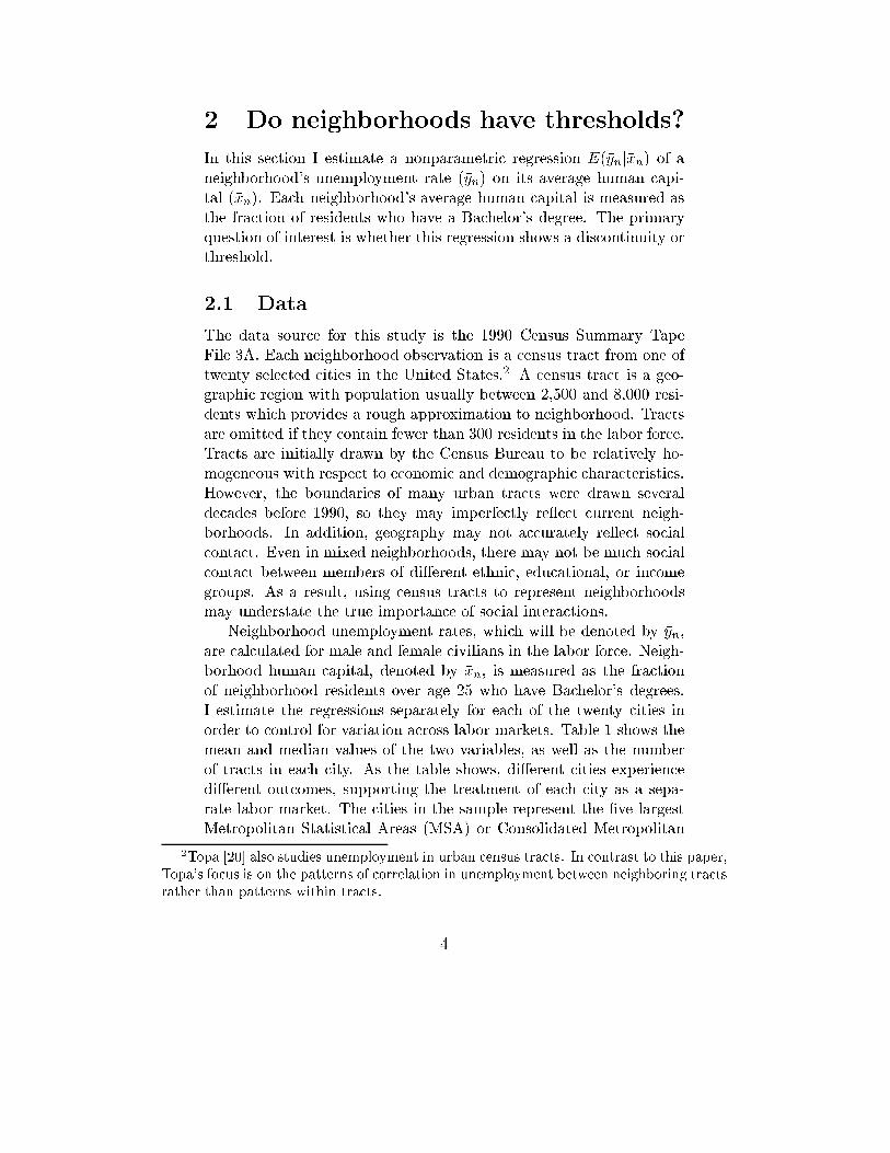
2 Do neighborhoods have thresholds?
In this section I estimate a nonparametric regression E(�ynj�xn) of aneighborhood's unemployment rate (�yn) on its average human capi-tal (�xn). Each neighborhood's average human capital is measured asthe fraction of residents who have a Bachelor's degree. The primaryquestion of interest is whether this regression shows a discontinuity orthreshold.
2.1 Data
The data source for this study is the 1990 Census Summary TapeFile 3A. Each neighborhood observation is a census tract from one oftwenty selected cities in the United States.2 A census tract is a geo-graphic region with population usually between 2,500 and 8,000 resi-dents which provides a rough approximation to neighborhood. Tractsare omitted if they contain fewer than 300 residents in the labor force.Tracts are initially drawn by the Census Bureau to be relatively ho-mogeneous with respect to economic and demographic characteristics.However, the boundaries of many urban tracts were drawn severaldecades before 1990, so they may imperfectly re ect current neigh-borhoods. In addition, geography may not accurately re ect socialcontact. Even in mixed neighborhoods, there may not be much socialcontact between members of di�erent ethnic, educational, or incomegroups. As a result, using census tracts to represent neighborhoodsmay understate the true importance of social interactions.
Neighborhood unemployment rates, which will be denoted by �yn,are calculated for male and female civilians in the labor force. Neigh-borhood human capital, denoted by �xn, is measured as the fractionof neighborhood residents over age 25 who have Bachelor's degrees.I estimate the regressions separately for each of the twenty cities inorder to control for variation across labor markets. Table 1 shows themean and median values of the two variables, as well as the numberof tracts in each city. As the table shows, di�erent cities experiencedi�erent outcomes, supporting the treatment of each city as a sepa-rate labor market. The cities in the sample represent the �ve largestMetropolitan Statistical Areas (MSA) or Consolidated Metropolitan
2Topa [20] also studies unemployment in urban census tracts. In contrast to this paper,Topa's focus is on the patterns of correlation in unemployment between neighboring tractsrather than patterns within tracts.
4

Statistical Areas (CMSA) in each of four regions - Northeast, Midwest,South, and West. An MSA is a primarily urban county or collectionof several contiguous counties. Each MSA is constructed by the Cen-sus Bureau to roughly represent a single labor market. A CMSA is acollection of contiguous metropolitan areas each of which is called aPrimary Metropolitan Statistical Area (PMSA). I use CMSA ratherthan PMSA or incorporated city in this paper for several reasons. Thepolitical boundaries of most major cities are generally much narrowerthan the corresponding metropolitan labor market, as evidenced bysubstantial commuting between city and suburbs. PMSA boundaries,while wider than city boundaries, tend to be inconsistent across di�er-ent metropolitan areas. For example, the Los Angeles - Long BeachPMSA contains only Los Angeles County, while the Houston PMSAcontains eight di�erent counties. A CMSA can include sparsely pop-ulated areas where a census tract is a poor proxy for a neighborhood.However, there are few such tracts relative to the number of urban-ized tracts, so the in uence of these tracts is slight. Estimation at thePMSA or county level (not reported) does not produce substantiallydi�erent results from those found using the entire CMSA.
2.2 Econometric issues
2.2.1 Identi�cation issues
The empirical relevance of neighborhood social interaction e�ects isa matter of substantial disagreement among social scientists. Manski[15] argues that this disagreement results from a fundamental problemof identi�cation. For example, we observe that a child is more likelyto smoke cigarettes if his friends smoke. This observation can beexplained by social interaction e�ects - he smokes because his friendssmoke. It can also be explained by \sorting" - he smokes because helikes to smoke, and he has made friends with fellow smokers. Theidenti�cation problem is that there is no way to tell the di�erence.Attempts to infer social interaction e�ects from behavior are subjectto this \sorting critique" whenever the neighborhood is selected bypurposive economic agents rather than by random experiment.
Social interaction e�ects and sorting have very di�erent policy im-plications. If there are true social interaction e�ects in unemployment,the residential distribution of individuals has an impact on individualemployment outcomes. Policies such as the Chicago Housing Author-
5

# of % w/Bachelors Unemployment %City Tracts Mean Median Mean Median
Baltimore 566 21.1 18.0 5.8 3.8Boston 1158 25.7 22.1 7.6 6.3New York 4813 23.4 19.5 7.6 5.7Philadelphia 1424 21.9 17.4 6.1 4.2Washington, D.C. 887 36.3 35.0 4.4 3.1Chicago 1841 20.3 14.4 9.8 5.9Cleveland 809 16.7 11.9 9.0 5.4Detroit 1239 17.6 12.4 10.5 6.6Minneapolis - St. Paul 612 25.2 21.5 5.3 4.3St. Louis 443 18.5 13.6 8.3 5.7Atlanta 469 24.4 20.1 6.2 4.5Dallas - Ft. Worth 816 24.8 21.3 6.7 5.2Houston 780 20.7 14.7 7.7 6.3Miami - Ft. Lauderdale 424 18.1 14.1 7.5 6.6Tampa - St. Petersburg 400 16.6 13.8 5.8 4.8Los Angeles 2504 21.8 18.3 6.9 5.9Phoenix 455 21.7 20.1 6.4 5.4San Diego 421 24.1 20.9 6.3 5.5San Francisco - Oakland 1281 30.4 27.8 5.5 4.4Seattle 511 26.1 22.7 4.9 4.1
Table 1: Summary statistics for the 1990 Census, by city.
6

ity's attempts to relocate public housing tenants into more economi-cally diverse neighborhoods [17] are based in part on the belief that theresidential concentration of the very poor produces a socially isolated\underclass" with little hope of better economic outcomes. The e�ec-tiveness of such a policy depends critically on the existence of econom-ically signi�cant social interaction e�ects. As a result, distinguishingbetween social interaction e�ects and sorting e�ects is important forthe development of social policy.
One approach to identi�cation is to ask individuals directly howthey make choices. In many cases, survey data on how individualsmake choices provides direct support for some degree of peer in uence.For the case of employment, survey data indicate that around half ofworkers �nd their jobs through referrals from employed friends, family,and neighbors [8]. However, the fact that individuals often use socialresources in job �nding does not say much about their employmentprospects in the absence of these resources.
In order to address the question of economic importance, one mustcompare the experience of observationally similar people in di�erentsocial environments. In most of the empirical literature on neighbor-hood e�ects, this takes the form of estimating a probit or logit modelon individual data linked with information on the person's neighbor-hood:
Pr(yi = 1jxi; �xn) = � (�0 + �1xi + �2�xn) (1)
where yi is the outcome, xi is a vector of individual characteristics,and �xn is some variable describing neighborhood composition. It istempting to say that the coeÆcient �2 measures the social interac-tion e�ect, but it actually measures the combined social interactione�ect and sorting e�ect. The identi�cation problem is that additionalassumptions are needed to estimate the two e�ects separately.
The most common assumption is exogenous selection into neigh-borhoods. Exogenous selection means that any individual character-istics which a�ect both neighborhood and the outcome in questionare included in the regressors. In this case, there is no sorting ef-fect (though there may be sorting), and �2 is the social interactione�ect. Unfortunately, the assumption of exogenous selection is dif-�cult to justify in most economically interesting cases. It would besurprising if school dropout, criminal behavior, public aid receipt, orout-of-wedlock childbearing did not a�ect neighborhood choice, yetthose are among the primary individual outcomes analyzed in this lit-erature. If the outcome itself a�ects neighborhood choice, any variable
7
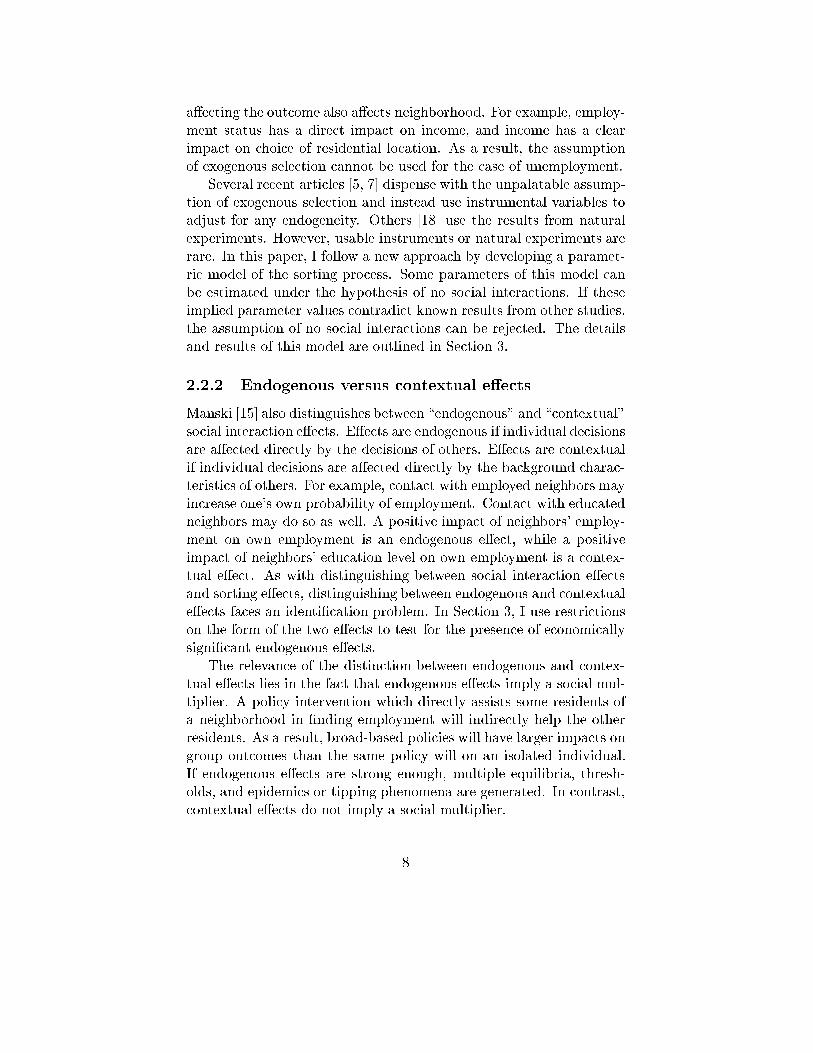
a�ecting the outcome also a�ects neighborhood. For example, employ-ment status has a direct impact on income, and income has a clearimpact on choice of residential location. As a result, the assumptionof exogenous selection cannot be used for the case of unemployment.
Several recent articles [5, 7] dispense with the unpalatable assump-tion of exogenous selection and instead use instrumental variables toadjust for any endogeneity. Others [18] use the results from naturalexperiments. However, usable instruments or natural experiments arerare. In this paper, I follow a new approach by developing a paramet-ric model of the sorting process. Some parameters of this model canbe estimated under the hypothesis of no social interactions. If theseimplied parameter values contradict known results from other studies,the assumption of no social interactions can be rejected. The detailsand results of this model are outlined in Section 3.
2.2.2 Endogenous versus contextual e�ects
Manski [15] also distinguishes between \endogenous" and \contextual"social interaction e�ects. E�ects are endogenous if individual decisionsare a�ected directly by the decisions of others. E�ects are contextualif individual decisions are a�ected directly by the background charac-teristics of others. For example, contact with employed neighbors mayincrease one's own probability of employment. Contact with educatedneighbors may do so as well. A positive impact of neighbors' employ-ment on own employment is an endogenous e�ect, while a positiveimpact of neighbors' education level on own employment is a contex-tual e�ect. As with distinguishing between social interaction e�ectsand sorting e�ects, distinguishing between endogenous and contextuale�ects faces an identi�cation problem. In Section 3, I use restrictionson the form of the two e�ects to test for the presence of economicallysigni�cant endogenous e�ects.
The relevance of the distinction between endogenous and contex-tual e�ects lies in the fact that endogenous e�ects imply a social mul-tiplier. A policy intervention which directly assists some residents ofa neighborhood in �nding employment will indirectly help the otherresidents. As a result, broad-based policies will have larger impacts ongroup outcomes than the same policy will on an isolated individual.If endogenous e�ects are strong enough, multiple equilibria, thresh-olds, and epidemics or tipping phenomena are generated. In contrast,contextual e�ects do not imply a social multiplier.
8
2.2.3 Aggregation
Aggregate data on neighborhoods have many useful properties - mostnotably, the availability of large numbers of aggregates and the factthat the Census includes the entire population of neighborhoods in acity. Both of these features are exploited in this study to achieve veryhigh precision in estimates and to model the neighborhood formationprocess itself. Unfortunately, it is not possible in general to inferindividual-level parameters from aggregates.
The standard method for ascertaining the existence of social inter-action e�ects is to estimate Equation (1) using individual-level dataand test the null hypothesis �2 = 0. A nonparametric analogue wouldbe to estimate:
E(yijxi; �xn) (2)
The joint null hypothesis of exogenous selection and no social interac-tion e�ects is equivalent to:
H0 : E(yijxi; �xn = X)�E(yijxi; �xn = X 0) = 0 for all fX;X 0g (3)
This null hypothesis is easy to test using individual data, but can it betested using only neighborhood-level averages �yn and �xn? In general,no. However, if xi is a single binary variable, then:
E(�ynj�xn = X) = E (yijxi = 0; �xn = X) (4)
+ �xn [E (yijxi = 1; �xn = X)�E (yijxi = 0; �xn = X)]
Under the null hypothesis (3), Equation (4) is linear in �xn. In otherwords, as long as xi is a single binary variable, testing for the linearityof E(�ynj�xn) is analogous to testing �2 = 0 with individual data, thekey exercise in much of the previous literature.3
While any form of social interaction e�ect is of interest, thresholde�ects are of particular interest. A threshold nonlinearity in principleis simply a discontinuity in the regression function. However, it is dif-�cult in practice to empirically distinguish a discontinuous regressionfunction (Figure 1) from one that has a steep slope over a short rangeof the dependent variable (Figure 2). As a result, any continuous re-gression function that shows a large change in unemployment over asmall range of neighborhood average human capital can be said to
3If E(yijxi; �xn) is linear and strictly monotonic in �xn, then E(�ynj�xn) will also be linear.The aggregate test will fail to reject the null hypothesis (3) , even though it is false andwould be rejected by the individual-level test.
9

provide evidence for neighborhood thresholds. No formal criteria forwhether a particular change is \large" will be de�ned; instead thatjudgment is left to the reader.
Pct.With.Bachelors
Une
mpl
oym
ent.R
ate
0 20 40 60 80 100
0.0
0.4
0.8
Figure 1: An example of a threshold relationship between two variables.
2.3 Baseline results
Figure 3 shows a scatter plot of neighborhood unemployment (�yn) ver-sus neighborhood educational attainment (�xn) for the Chicago CMSA.The �gure shows an interesting set of patterns which appear in theother cities as well. For neighborhoods with more than twenty percentcollege graduates, unemployment rates are uniformly low. In contrast,neighborhoods with fewer than twenty percent college graduates ap-pear to have much higher average unemployment rates as well as muchhigher variability in unemployment.
Figures 4 through 7 show nonparametric regressions of neighbor-hood unemployment on neighborhood human capital for each of thecities in the sample. These estimates are calculated using the super-smoother [9, page 181], and the 95 percent con�dence intervals shownare estimated by the bootstrap with 1,000 iterations.4 As appears in
4To describe the procedure in more detail, I estimate a series of X% pointwise intervals,then increase the value ofX until 95% of the bootstrapped regression functions are entirelywithin these intervals (see H�ardle [9] for a discussion of this procedure). As a result, thecon�dence interval has a 95% probability of containing the entire true regression function.
10

Pct.With.Bachelors
Une
mpl
oym
ent.R
ate
0 20 40 60 80 100
0.0
0.4
0.8
Pct.With.Bachelors
Une
mpl
oym
ent.R
ate
0 20 40 60 80 100
0.0
0.4
0.8
Figure 2: Examples of regression relationships which provide evidence forthresholds.
.. . ..... . ... .. .... . ... . .. ... .
.. .
... . .
.... .. ... ...... . .... .... ...
.. . .. .. .. .. .. .... .. ....
... . . . ... . .. ... ..
.. . ... .. ... . ... ..
.
.
..
.
. . . .. .... .
.
.. ... . ... .... .. .. .. ....
.. ...... .. ...... ... ... . .... .. . .....
... ..... ... ... . ...... .... . ....... ............ ....
... .
.
.. . ... . ...
. .....
.... .... .... . .
..
.
..
. ..
... .. .. .
.....
... . . . ...
.
....... ... ...
... .
... .. .........
...
...... ...
.
...
.
...
.....
. ..
.. .
..
.
.
..
.
.
....
.
.
..
..
. .. . ..
.
..
.. .
.
.
.
.
.
.
.
.
.
.
..
.
.
....
.....
. .
.
.. ....
....
.. ...... ..........
...... ..... ..
. .. ...
..
..
.. ..
.
.
.
.
.
..
.. .
. ..
..
.
.
.
....
....
..
..
..... .
.
.
..
.
.... ..
. ...
.
.
..... .
. .... . ... . ..
...
.. ..... .. .
. ..
.. . .. ...
. .... . ....... ..
.. .
. ... ..
. .. .. ..
.....
.. ...
. ... ..
.. . . ...... ..
. .. ...
.
....
... ......... ... .. ..... ... ... .. . ... ...... .. .
.. . .. ....
...... ...
.. ..
....
.....
. ...
.
... ......... .. .
.
.... ... .. .
.......
.........
. ..........
........
. .. .... .
.. .
..
.
.. .. .
. ...... .. .. ...... .. . ....
.....
. ....
.....
.
.
.... .... .. . .. .... . . ...... .... .. .. .. . ...
... .. . .. .. .. .. .. ... .... . .. .. .. . .. .. ... . .. .. . ... .... .. . ... . ... .... . ... . . ....... . . .. .. . ... .... ..... . . ..... .. ... ... ..... .. .. ... ... . ... . .. .. . .... . ..... .. .. .. . . ..... ...... ... ..... ..... . . ... .. ... .. ... .. ...
... ... ... . .. ..... .. . ... ...... .... ....... .
.... .. . .. . ..... . ... .. . . . .. ..... ....... .... .... ... ..
...... . ..... . . .. .. .... ... .... ..
.
.... .. ... . .... . ...... .... . . .... ... . .. . . ..
. .. ........ . .. . ... .. ...
. ...
.
..... . ... ... .. .. .... .. . ... ...
.
. ..
.....
... .. . . . .. ..... ... .. .... . .... . .. .. ... ... .... . . ... .. .... . . ... .. . .. . .. ........ . . .. .. . .... .. .. ..... . . ..... . .... . . ... .. ... .. ... ... . ... ..... ......
.... . .. ... ..
. .
.. ..... ... .. .... ... . .. . .. .. . .. ........
.. .... ... . .. .. ... ...... ... .. ..... . . .. ... .... ... .. ....... ..
... .... . ... . .... .. . .... . .... .. .. . .. . . ... . .. ... ... ... .. . ........ . .. . .... . ... . ... .. .. . ... . .. ... ... . ..... .. . ... .. .......
..
. .. ....
. ....
. ..... ... ..... .. .... ... ... ....
. . ... .. ..
.
. ..
....... .
...
.
.
.
..
. ...... .....
.. .
.. . ... ....
.
.
.
. ... ...
.. . ...... ... .
.. .... ... .. .. .. ... .. .. .... . ... ... ..... .... . .... ...
..... ... . .
... .. ....... .
Chicago
Pct.With.Bachelors
Une
mpl
oym
ent.R
ate
0 20 40 60 80 100
0.0
0.4
0.8
Figure 3: Scatter plot of neighborhood unemployment versus neighborhoodeducation in Chicago CMSA.
11

the scatter plot, the regression relationship is noticeably nonlinear,and almost every city exhibits a clear threshold. The predicted unem-ployment rate increases substantially when the percentage of collegegraduates in a neighborhood falls below about twenty. This thresholdis consistent with epidemic models of social interactions.
The apparent nonlinearity of the regressions can be placed in amore formal statistical setting. I test for the linearity of each re-gression using H�ardle and Mammen's nonparametric method [10] fortesting the linearity of a conditional expectation function. The proce-dure is to estimate the CEF both nonparametrically and with OLS.The average Euclidean distance between the two estimators at eachpoint of the support, with a few bias corrections described in theirpaper, is then the test statistic. H�ardle and Mammen show that thistest statistic is consistent and asymptotically normal, but show that abootstrap estimator yields better small-sample estimates for the dis-tribution of the test statistic under the null hypothesis of linearity.Table 2 shows the estimated test statistic, critical value, and p-valuefor this linearity test by city. The test statistic is calculated as inH�ardle and Mammen, and its distribution under the null is estimatedusing the wild bootstrap with 1,000 iterations. As the table shows, lin-earity of E(�ynj�xn) is easily rejected by the data in all cases. As shownin Section 2.2.3, this also leads us to reject the related joint hypothesisof exogenous selection and no social interactions. At minimum, thereis some sorting e�ect or social interaction e�ect.
While linearity is easily placed within a formal hypothesis test set-ting, I have chosen to de�ne \threshold" informally as a large changein average outcome associated with a small change in the regressor.Establishing whether the true conditional expectation function fora given city is characterized by thresholds cannot be done formally.However, there is still convincing evidence that this is the case. Thethresholds appear across the many di�erent cities in this sample, andthe con�dence intervals for Figures 4 - 7 are quite narrow due to thelarge samples. This is strong statistical evidence that the thresholdshapes are characteristics of the underlying CEF.
Thresholds are a robust characteristic of the reduced form relation-ship between neighborhood resources and neighborhood unemploy-ment. This reduced-form result is consistent with epidemic modelsof social interaction e�ects. However, other structural models mayhave similar reduced-form implications. In Section 3, I consider alter-native explanations and argue that the epidemic explanation is more
12

Baltimore
Pct.With.Bachelors
Une
mpl
oym
ent.R
ate
0 20 40 60 80
0.05
0.15
Boston
Pct.With.Bachelors
Une
mpl
oym
ent.R
ate
0 20 40 60 80
0.05
0.15
New York
Pct.With.Bachelors
Une
mpl
oym
ent.R
ate
0 20 40 60 80
0.05
0.15
Philadelphia
Pct.With.Bachelors
Une
mpl
oym
ent.R
ate
0 20 40 60 80
0.02
0.08
0.14
Washington, D.C.
Pct.With.Bachelors
Une
mpl
oym
ent.R
ate
0 20 40 60 80
0.0
0.04
0.10
Figure 4: Nonparametric regressions for northeastern cities.
13

Chicago
Pct.With.Bachelors
Une
mpl
oym
ent.R
ate
0 20 40 60 80
0.0
0.10
0.20
Cleveland
Pct.With.Bachelors
Une
mpl
oym
ent.R
ate
0 20 40 60 80
0.0
0.10
0.20
Detroit
Pct.With.Bachelors
Une
mpl
oym
ent.R
ate
0 20 40 60 80
0.05
0.15
0.25
Minneapolis - St. Paul
Pct.With.Bachelors
Une
mpl
oym
ent.R
ate
0 20 40 60 80
0.04
0.08
St. Louis
Pct.With.Bachelors
Une
mpl
oym
ent.R
ate
0 20 40 60 80
0.05
0.15
Figure 5: Nonparametric regressions for midwestern cities.
14

Atlanta
Pct.With.Bachelors
Une
mpl
oym
ent.R
ate
0 20 40 60 80
0.05
0.15
Dallas - Ft. Worth
Pct.With.Bachelors
Une
mpl
oym
ent.R
ate
0 20 40 60 80
0.04
0.10
Houston
Pct.With.Bachelors
Une
mpl
oym
ent.R
ate
0 20 40 60 80
0.0
0.06
0.12
Miami - Ft. Lauderdale
Pct.With.Bachelors
Une
mpl
oym
ent.R
ate
0 20 40 60 80
0.02
0.08
0.14
Tampa - St. Petersburg
Pct.With.Bachelors
Une
mpl
oym
ent.R
ate
0 20 40 60 80
0.04
0.08
0.12
Figure 6: Nonparametric regressions for southern cities.
15

Los Angeles
Pct.With.Bachelors
Une
mpl
oym
ent.R
ate
0 20 40 60 80
0.0
0.06
0.12
Phoenix
Pct.With.Bachelors
Une
mpl
oym
ent.R
ate
0 20 40 60 80
0.04
0.10
San Diego
Pct.With.Bachelors
Une
mpl
oym
ent.R
ate
0 20 40 60 80
0.04
0.08
0.12
San Francisco - Oakland
Pct.With.Bachelors
Une
mpl
oym
ent.R
ate
0 20 40 60 80
0.02
0.08
Seattle
Pct.With.Bachelors
Une
mpl
oym
ent.R
ate
0 20 40 60 80
0.02
0.06
Figure 7: Nonparametric regressions for western cities.
16

plausible.
City Test 95% Critical P-valueStatistic Value
Baltimore 0.338 0.0139 0Boston 0.359 0.00512 0New York 1.76 0.000696 0Philadelphia 1.02 0.0101 0Washington, D.C. 0.337 0.0137 0Chicago 3.45 0.00449 0Cleveland 1.52 0.0207 0Detroit 1.59 0.00242 0Minneapolis - St. Paul 0.862 0.00924 0St. Louis 0.356 0.0144 0Atlanta 0.108 0.00236 0Dallas - Ft. Worth 0.346 0.00214 0Houston 0.0586 0.000758 0Miami - Ft. Lauderdale 0.0989 0.00598 0Tampa - St. Petersburg 0.083 0.0221 0Los Angeles 0.444 0.000594 0Phoenix 0.476 0.0117 0San Diego 0.00191 0.00064 0San Francisco - Oakland 0.245 0.00139 0Seattle 0.0572 0.00862 0
Table 2: Results from H�ardle-Mammen test for linearity of E(�ynj�xn)
3 Alternative explanations, sorting, and
misspeci�cation
In general, separate identi�cation of sorting e�ects and true social in-teraction e�ects cannot be made from observations on behavior with-out strong identifying restrictions on the nature of the e�ects. Theprevious section established that either sorting e�ects or social inter-action e�ects must be present. In this section, I apply a new strategy
17

to distinguish between the two types of e�ects.
3.1 How do individuals sort?
The residential location choice made by individuals and families isin uenced by many family characteristics { current location, income,taste for housing quality, family size, presence of family or social ties,ethnicity, and many others. However, only those factors which canlead to mistaken inference of social interactions are of interest for thispaper. In order to do so, a candidate sorting variable must be cor-related with neighborhood educational level and also help to improvepredictions of employment probability after controlling for individualeducation level. For example, sorting on educational attainment can-not produce spurious thresholds, since this is the independent variable.Another alternative is that individuals sort on employment status it-self. Taken literally, this implies that the distribution of neighborhoodunemployment rates should have many neighborhoods with no unem-ployment and a few neighborhoods with unemployment of 100 percent.Yet nearly all of the neighborhoods in my sample have unemploymentrates which strictly between zero and thirty percent. Direct sortingon employment status can thus be ruled out.
A more promising candidate is that families sort on income. In asimple housing market with no externalities, neighborhood strati�ca-tion on income level will occur if the most attractive and expensivehousing locations are in the same neighborhood. As housing is anormal good, high-income families will choose to live in the most at-tractive neighborhood.5 However, they are unlikely to sort exclusivelyon current income. More than half of the sample lived in the samelocation in 1985 and 1990, and even the highest-education neighbor-hoods had some unemployment. These two facts suggest that familiesdo not always change residential location in response to a transitorychange in income or employment. Indeed, if families face moving costs,or if they simply wish to smooth their consumption of housing andneighborhood resources, they choose residential location on the ba-sis of more long-term income prospects. In the remainder of Section3, I use an indirect approach to exploit the idea that the primary
5In the presence of quantitatively important social interaction e�ects, the neighborhoodformation problem becomes more complex because families care who their neighbors are.B�enabou [1] and Durlauf [4] describe conditions under which social interaction e�ectsreinforce the incentive to sort.
18

determinant of neighborhood choice is a family's long-term incomeprospects, which I refer to as their \productivity." Note that produc-tivity should not be interpreted as innate ability, IQ, education, ora test score. Instead, productivity includes any characteristics of theworker which a�ect the worker's income-generating ability which arepermanent and portable.
3.2 A simple model
In this section, I develop a model in which each individual's employ-ment outcome is described by a simple binary choice model and indi-viduals sort into neighborhoods on an unobserved productivity vari-able. Even with these assumptions separate identi�cation of sortingand social interaction e�ects is not possible. Instead, I assume thatthere is no social interaction e�ect, estimate the model in which sort-ing must explain the threshold, and evaluate the resulting estimatesfor plausibility.
In the model, each of the I workers in a given city is characterizedby education xi and productivity zi 2 [0; 1], both of which are exoge-nous. As described above, a worker's productivity level is his or herlong-term income-generating ability, measured in dollars. Educationlevel is binary:
xi =
(0 if no college degree1 if college degree
These two characteristics are distributed jointly across individualswith distribution function F . The conditional distribution F (zijxi)has a strictly monotone likelihood ratio, i.e., an individual with a col-lege degree is more likely to have higher productivity. Each workergoes through a two-step process:
1. Worker chooses a neighborhood based on a simple sorting rule.Workers stratify perfectly into N neighborhoods of equal sizebased on their value of zi. In other words, neighborhood onecontains the individuals with the I=N lowest realizations of zi,neighborhood two contains the I=N next lowest, etc. For simplic-ity, assume that I=N is an integer and that any ties are brokenby lottery.
2. Worker receives a random employment o�er and accepts or re-
19

jects it, producing the binary employment outcome yi, where
yi =
(0 if accept (employed)1 if reject (unemployed)
Let �xn represent the neighborhood average of xi, and de�ne �yn and�zn similarly. The net wage o�er (wage o�er minus reservation wage)is linear in education, productivity, and any neighborhood variables:
wi = �0 + �1xi + �2�xn � �3�yn + �4zi + ��n + �i (5)
The coeÆcient on �xn thus corresponds to the contextual neighbor-hood e�ect, and the coeÆcient on �yn corresponds to the endogenousneighborhood e�ect. As workers sort into neighborhoods on zi, itscoeÆcient corresponds to the sorting e�ect.
The worker accepts the net wage o�er wi if it is positive, or if thegross wage o�er exceeds his or her reservation wage.
yi =
(0 if wi � 01 if wi < 0
(6)
The variables ��n and �i represent unobserved neighborhood andindividual level shocks, respectively. Unlike the unobserved produc-tivity variable zi, which is known by the worker before choosing loca-tion, the shocks ��n and �i a�ect the worker after the locational choicehas been made. I assume the neighborhood level shock is mean-zeroconditional on the other neighborhood characteristics, though it maybe heteroscedastic:
E(��njxi; zi; �i 8i in neighborhood) = 0 (7)
I also assume that �i is independent and identically distributed acrossindividuals, is independent of individual characteristics, and has alogistic distribution. Unemployment thus follows a logit model:
Pr(yi = 1jxi; zi; �xn; �yn; ��n) = � (�(�0 + �1xi + �2�xn � �3�yn + �4zi + ��n))(8)
where:
� (X) � Pr(�i � X) =eX
1 + eX
Note that equation (8) includes the individual-level variables xi andzi, while the data consist of neighborhood-level proportions. The as-sumptions of the sorting model allow equation (8) to be rewrittenentirely in terms of aggregates.
20
For a large economy, the sorting model implies a strictly mono-tonic function z (�xn) such that every worker in a neighborhood witha fraction �xn of college graduates has productivity level zi = z (�xn).Equation (8) becomes:
Pr(yi = 1jxi; zi; �xn; �yn; ��n) = � (�(�0 + �1xi + �2�xn � �3�yn + �4z (�xn) + ��n))(9)
It is thus possible in principle to distinguish between zi, ��n, and �i,because zi has a functional relationship with �xn, but ��n and �i areuncorrelated with �xn. The source of distinction is that zi a�ects resi-dential choice and ��n + �i does not.
If the neighborhood is large, �yn converges to its expected value,producing the following aggregate structural model:
�yn = �xn � � (�(�0 + �1 + �2�xn � �3�yn + �4z (�xn) + ��n)) (10)
+ (1� �xn) � � (�(�0 + �2�xn + �3�yn + �4z (�xn) + ��n))
The approximation that �yn = E(�yn) is reasonable for a census tract asthe standard deviation of an average of a few thousand independentand identically distributed Bernoulli random variables is quite small.For example, in the median tract in Chicago, with about 2400 adultsin the labor force and 6% unemployment, the standard deviation isless than one half of one percentage point.
Equation (10) will be used as the basis for estimation in this sec-tion. The parameters of interest are �2 (the contextual e�ect) and�3 (the endogenous e�ect), as well as the function �4z (�xn) (the sort-ing e�ect). Because both zi and ��n are unobserved, substantial fur-ther identifying restrictions on the data-generating process would beneeded to estimate the relevant parameters. Instead, I follow a moreindirect strategy. I isolate each of the three e�ects (contextual, en-dogenous, and sorting) in turn by assuming the other two e�ects arenot present. I then estimate the model under that restriction, andevaluate how well the resulting model �ts the joint distribution of �ynand �xn. Although it is likely that all three e�ects are present to someextent, this procedure will identify which e�ects must be present inorder to �t the data. In Section 3.3, I evaluate how sorting explainsthe data in the absence of true social interactions. In Section 3.4, Icompare how well contextual and endogenous e�ects explain the datain the absence of sorting. In the interests of space, I show results forthe Chicago CMSA only. Chicago has been studied at the neighbor-hood level more than any other U.S. city [20, 21, 22], and the resultsin other cities (available from the author) are quite similar.
21

3.3 Can sorting generate thresholds?
In this section I assume that there are no social interaction e�ects, andevaluate whether sorting alone can plausibly generate the thresholdsseen in the data. I �nd that sorting can generate thresholds, but onlyunder an implausible distribution for the productivity variable.
Assume no social interaction e�ects (�2 = �3 = 0), and �x thedirect bene�t of education at zero (�1 = 0).6 Under these restrictions,equation (10) reduces to the following:
�yn = �(�(�0 + �4z (�xn) + ��n)) (11)
A particularly convenient transformation is to take the log odds ratioof both sides. The log odds ratio function is simply the inverse of thelogistic function:
��1 (X) = ln(X) � ln(1�X) (12)
Applying the transformation to (11):
���1 (�yn) = �0 + �4z (�xn) + ��n (13)
Taking expectations and rearranging:
z (�xn) =E(���1 (�yn) j�xn)� �0
�4(14)
Equation (14) implies that a linear transformation of z (�xn) can beidenti�ed from the data. Figure 8 shows the estimated z (�xn) for theChicago CMSA. As the �gure shows, z (�xn) must be substantiallynonlinear if it is to generate the observed threshold in the regressionrelationship.
Because the distribution of �xn is observed for each city, z (�xn) alsoimplies a distribution of zi across individuals. Since zi represents aworker's general productivity, the shape of that distribution should beplausible for productivity. Figure 9 shows the empirical distributionof college degrees across neighborhoods in the Chicago CMSA. Asthe �gure shows, this distribution is positively skewed. Figure 10shows the distribution of productivity across individuals implied bythe estimated z (�xn) As the �gure shows, the implied distribution ofproductivity is symmetric or negatively skewed.
6I show in Appendix A that this assumption is innocuous, but makes the algebra muchclearer.
22

This implied distribution can be compared to independent esti-mates of the distribution of productivity across the economy. It iswell known that the distribution of wages is not symmetric but is pos-itively skewed. In a competitive labor market with no frictions, thedistribution of wages and the distribution of marginal productivityare identical. However, a labor market without frictions is a strongassumption, especially in a study of unemployment. In the presence ofcostly search, workers are not necessarily paid their marginal product,so wages and productivity do not necessarily have identical distribu-tions. Koning, Ridder, and van den Berg [13] estimate the distributionof productivity in the context of an equilibrium search model. They�nd a distribution which is highly positively skewed. This suggeststhat a productivity distribution should not be symmetric but ratherskewed.
Could a positively skewed distribution of zi generate a nonlinearz (�xn) like that shown in Figure 8? The sorting process describedearlier implies that if a neighborhood's productivity level �zn is in per-centile X of the productivity distribution, its average educational at-tainment �xn must be exactly in percentile X of its distribution:
Fx(�xn) = Fz(�zn) (15)
Suppose both distributions are skewed as in Figures 9 and 10. When�xn is low, F 0
x is high and F 0
z is low. Relatively large percentile in-creases are associated with small increases in �xn, while the opposite istrue for �zn. In the Chicago CMSA, the di�erence in �xn between theworst-educated neighborhood and the median neighborhood is about15 percentage points, while the di�erence between the median and thebest is about 85. In contrast, when �zn is in its lower two quartiles, F 0
z
is low - a relatively large change in �zn is needed to generate a moderatechange in percentile terms. So a small increase in �xn leads to a largerincrease in percentile terms which leads to an even larger increase in�zn. When �xn is high, the reverse logic applies, generating a steep slopein z (�xn) when �xn is low and a at slope when it is high. If both dis-tributions are skewed in the same direction, there will be no thresholdrelationship. In particular, if the distributions have the same shape(Fx(X) = Fz(aX) for some constant a), then the relationship impliedby equation (15) will be exactly linear.
To summarize, a z (�xn) function which generates the observed re-lationship between unemployment and education without social in-teractions requires that unobserved productivity have a roughly sym-
23

Chicago
Pct.With.Bachelors
Uno
bser
ved
Pro
duct
ivity
0 20 40 60 80 100
0.0
0.4
0.8
Figure 8: Estimated z (�xn) for Chicago. �0 and �4 set so that range of z (�xn)is [0; 1].
Chicago
Pct.With.Bachelors
Pro
babi
lity
dens
ity
0 20 40 60 80
0.0
0.02
0.04
Figure 9: Distribution of �xn across neighborhoods in Chicago.
24

Chicago
Unobserved productivity
Pro
babi
lity
dens
ity0.0 0.2 0.4 0.6 0.8 1.0
0.2
0.8
1.4
Figure 10: Distribution of zi across individuals in Chicago, for estimatedz (�xn).
metric or negatively skewed distribution, like that shown in Figure 10.A more plausibly shaped distribution for productivity is a positivelyskewed one similar to that shown in Figure 9, and this distributiongenerates a linear z (�xn), which is rejected by the data. I thus concludethat sorting alone does not generate the kind of thresholds observedin the data.
3.4 Contextual vs. endogenous e�ects
In this section I that assume there is no sorting e�ect, and evaluatewhether contextual or endogenous neighborhood e�ects can plausiblygenerate the thresholds seen in the data.
To isolate the contextual e�ect, I assume that the endogenous andsorting e�ects are zero (�3 = �4 = 0). I also �x the direct e�ect ofeducation at zero (�1 = 0). Under these restrictions, equation (10)reduces to the following:
�yn = �(�(�0 + �2�xn + ��n)) (16)
Equation (16) can be estimated from neighborhood data. Applyingthe log odds transformation to both sides produces:
��1 (�yn) = �(�0 + �2�xn + ��n) (17)
25

so a linear contextual e�ect translates into a linear relationship be-tween neighborhood educational attainment and the log odds ratiotransformation of the unemployment rate.
To isolate the endogenous e�ect, I assume that the contextual andsorting e�ects are zero (�2 = �4 = 0). These restrictions generate thefollowing reduced form:
�yn = �xn � � (�(�0 + �1 + �3�yn + ��n)) (18)
+ (1� �xn) � � (�(�0 + �3�yn + ��n))
Note that equation (18) has �yn on both sides, so the implied relation-ship between �yn and �xn must be solved as a �xed point or equilibriumproblem. Brock and Durlauf [2] analyze a class of models which in-cludes equation (18) and prove that if �3 is large enough, the resultingequilibrium correspondence �yn(�xn) will exhibit multiple equilibria andthreshold behavior in a critical range. While multiple equilibria pre-clude identi�cation of the exact coeÆcients in equation (18), thresh-old behavior will also carry over to the log odds ratio transformation.Strong endogenous e�ects thus imply that the regression relationshipE(��1 (�yn) j�xn) is nonlinear, while linear contextual e�ects imply itis linear. As a result, distinguishing between endogenous e�ects andlinear contextual e�ects can thus be done by testing for nonlinearityin the log odds ratio.7
I apply the H�ardle-Mammen test described earlier to test the nullhypothesis that E(��1 (�yn) j�xn) is linear against the alternative thatit is not.8 I �nd that linearity is rejected for all cities. Combinedwith the results in the previous section, this provides evidence that aneconomically relevant endogenous e�ect is present.
4 Extensions
4.1 Race
Because this study is restricted to a single explanatory variable, miss-ing variables are of substantial concern. In addition to the indirectmethodology pursued in the previous section, it would be useful tocontrol directly for variables that are known to a�ect employment
7This result was pointed out to me by William A. Brock.8Note that this test is limited in that it can only reject a linear contextual e�ects model.
It has no power to reject a nonlinear contextual e�ect or any type of endogenous e�ect.
26

Ch
icag
o
Pct.W
ith.B
ach
elo
rs
log odds ratio(unemployment)0
20
40
60
80
-3.5 -2.5 -1.5
Figu
re11:
Estim
atedE(�
�1(�y
n )j�x
n )for
Chicago
CMSA.
rates.Twocan
didate
missin
gvariab
lesare
ageandrace.
Unem
ploy
-mentrates
fortheyou
ngandfor
African
American
sare
both
substan
-tially
high
erthan
average[11
,Table16.5].
Ifeith
erof
these
variables
issystem
aticallyrelated
tothepercen
tageof
collegegrad
uates
ina
neigh
borh
ood,then
thisrelation
ship
could
induce
aspuriou
sthresh
-old
.Manyof
thestan
dard
meth
odsof
controllin
gfor
agiven
variable
areprob
lematic
inthiscon
text.
Onecom
mon
practice
isto
orthogo-
nalize
thedependentvariab
lewith
respect
totheoth
erneigh
borh
ood
characteristics
andtreat
thisresid
ualas
thequantity
ofinterest.
Un-
der
thehypoth
esisof
endogen
oussocial
interaction
s,how
ever,neigh
-borh
oodunem
ploy
mententers
into
individual
unem
ploy
mentprob
a-bilities
inahigh
lynonlin
earway,
creatingathresh
old.Becau
seany
other
relevantvariab
lewould
alsohave
thisnonlin
earsocial
multip
liere�ect,
thestan
dard
practice
isinvalid
precisely
under
thecon
dition
sofinterest.
Inthissection
andin
Section
4.2,Idiscu
sstwoapproach
eswhich
overcomethelim
itationsof
thestan
dard
practice.
Tosee
how
racialdi�eren
cesin
employ
mentpattern
sare
suÆcien
tto
generate
thresh
olds,con
sider
thefollow
ingexam
ple.
There
areno
social
interaction
s,andtheonly
individual
variables
that
matter
forem
ploy
mentare
raceandeducation
.Theunem
ploy
mentrates
ofthe
fourgrou
psare:P
r(yi=1jb
lack,college
degree)
=0:10
27

Pr(yi = 1jblack, no college degree) = 0:20
Pr(yi = 1jwhite, college degree) = 0:05
Pr(yi = 1jwhite, no college degree) = 0:15
Suppose also that neighborhoods are completely racially segregated.Within neighborhoods of a particular race, the aggregate employment-education relationship is linear, as shown by the dotted lines in Figure12. Now suppose that all neighborhoods with fewer than 10 percentcollege graduates are all black and all neighborhoods with more than10 percent are all white. The resulting aggregate relationship between�xn and �yn will then look like the solid line in Figure 12, even thoughthere are no social interaction e�ects. While this example is extreme,it illustrates that a relationship between percent black and average ed-ucational attainment in neighborhoods can lead to spurious inferenceof social interaction e�ects.
Pct.With.Bachelors
Une
mpl
oym
ent.R
ate
0.0 0.2 0.4 0.6 0.8 1.0
0.05
0.15 blacks
whites
Figure 12: Example of spurious threshold due to ethnic group di�erences inunemployment rates.
Fortunately, the Census provides a breakdown of both educationand employment status in a neighborhood by racial category. Let �xbnbe the fraction of black residents of neighborhood n who are collegegraduates, and �ybn be their unemployment rate. De�ne �xwn and �ywn simi-larly for white residents. If the argument above is empirically relevant,then E(�ybnj�x
bn) and E(�ywn j�x
wn ) will both be linear. Figure 13 shows the
28

estimated regressions by racial category for the Chicago CMSA. Al-though unemployment rates are signi�cantly higher among blacks, thethreshold remains for both blacks and whites. The threshold remainsfor the fourteen other cities which had signi�cant African-Americanpopulations. 9 In addition, I perform H�ardle-Mammen linearity testsand �nd that linearity is rejected for all fourteen cities. Accounting forthe impact of simple di�erences in neighborhood racial compositiondoes not a�ect the results of Section 3.
Chicago
White onlyPct.With.Bachelors
Une
mpl
oym
ent.R
ate
0 20 40 60 80
0.02
0.06
0.10
0.14
Chicago
Black onlyPct.With.Bachelors
Une
mpl
oym
ent.R
ate
0 20 40 60 80
0.1
0.2
0.3
Figure 13: Nonparametric regressions by racial category. First graph showsestimated regression for whites, second shows regression for blacks.
4.2 Racial segregation
A related alternative hypothesis is that educational segregation is aproxy variable for racial segregation, and that racial segregation itselfhas negative e�ects on employment outcomes. The relative impor-tance of segregation by race and by economic status in exacerbatingblack poverty is a matter of active current debate,10 so this alternativeform of social interaction e�ect should be considered. The distinction
9Six cities { Boston, Minneapolis - St. Paul, Phoenix, Tampa - St. Petersburg, SanDiego, and Seattle { were dropped because they have few black residents.
10The work of Massey and Denton [16, and others] argues in favor of the view that racialsegregation matters most, in contrast to Wilson's [21] focus on economic segregation.
29

between the employment e�ect of being black and the e�ect of livingin a majority-black neighborhood is subtle, but can be investigatedseparately in this case. To do so, I split each city in my sample intothose census tracts which are majority black and those which are not.The distribution of percent black in a neighborhood is bimodal in thesample, and almost all neighborhoods can be clearly categorized ashaving mostly black or mostly white residents. I estimate the basicregression E(�ynj�xn) for each subsample separately. Again, six citieswere dropped from the analysis. The results for the Chicago CMSAare shown in Figure 14. As the �gure shows, the apparent thresh-old is much more prominent for majority-black neighborhoods. Thislends some support to the argument that majority-black neighbor-hoods have unique characteristics. However, both thresholds remain,so the thresholds themselves are not an artifact of racial segregation.Again, H�ardle-Mammen tests reject linearity for all fourteen cities.
Chicago
Majority black neighborhoodPct.With.Bachelors
Une
mpl
oym
ent.R
ate
0 20 40 60 80
0.1
0.2
0.3
0.4
Chicago
Majority white neighborhoodPct.With.Bachelors
Une
mpl
oym
ent.R
ate
0 20 40 60 80
0.02
0.06
0.10
0.14
Figure 14: Nonparametric regressions by racial majority in neighborhood.
4.3 Age
The unemployment rate of individuals between 16 and 24 years ofage is roughly twice that of those between 25 and 64. If the fractionof young adults in a community varies systematically with the edu-cational attainment of its older members, the age distribution of theneighborhood could be an important missing variable. In addition,
30

as education level is calculated for residents over age 25 and unem-ployment is calculated for residents over 16, these variables do notcover exactly the same populations as assumed in previous sections.Unemployment for those in the 25-64 age range would be a preferabledependent variable, but is unavailable at the tract level. To addressthis issue, I solve for bounds on the true regression function.
Let �yan be the unemployment rate for individuals in age range aand let p be the proportion of the labor force below age 25.
�y16�64n = �y25�64n � (1� p) + �y16�24n � p (19)
Solving this equation for the variable of interest, the unemploymentrate of 25-64 year-olds:
�y25�64n =�y16�64n � �y16�24n � p
1� p(20)
The unemployment rate �y16�64n and population proportion p are ob-served in the data for each tract, but the youth unemployment rate�y16�24n is not. Because unemployment rates are higher for youth, theunemployment rate of 16-64 year-olds is an upwardly biased estimateof the unemployment rate of 25-64 year-olds.
While the data do not show unemployment rates for either agegroup, suppose there is a plausible upper bound on youth unemploy-ment �y16�24n .
�y16�24n � �ymax
n
As equation (20) is monotonic in �y16�64n , this restriction implies a lowerbound on unemployment for adult workers.
�y25�64n ��y16�64n � �ymax
n � p
1� p(21)
The upper bound is simply the measured unemployment rate for thetract. Once the bounds are calculated for each tract, the desirednonparametric regression function E(�y25�64n j�xn) can be bounded:
E(�y16�64n � �ymax
n � p
1� pj�xn) � E(�y25�64n j�xn) � E(�y16�64n j�xn) (22)
The constraint that the adult unemployment rate cannot be less thanzero may bind as well. Provided that we set an upper bound on youthunemployment, the upper and lower bounds of equation (22) can beestimated.
31

Figure 15 shows estimated regression bounds for the Chicago CMSA.The �rst depicts the worst-case scenario of 100% youth unemployment,the second depicts bounds for 50% youth unemployment. Of the tractsin Chicago, only nine have unemployment rates higher than �fty per-cent, although the number with youth unemployment rates above �ftypercent is likely to be higher. The appropriate interpretation of thesebounds is di�erent from that of a con�dence interval. Any regressionfunction that can be drawn between the upper and lower bound isconsistent with the data, and there is no well-de�ned sense in whichany such function is \more likely" than any other such function. Asthe �gure shows, for the worst-case bounds, we cannot reject a linearrelationship between neighborhood education and neighborhood un-employment. However, if the youth unemployment rate is no morethan �fty percent in each tract, a linear relationship can be rejected.
Chicago
bounds for up to 100 % teen unemploymentPct.With.Bachelors
Une
mpl
oym
ent.R
ate
0 20 40 60 80
0.0
0.10
0.20
Chicago
bounds for up to 50 % teen unemploymentPct.With.Bachelors
Une
mpl
oym
ent.R
ate
0 20 40 60 80
0.0
0.10
0.20
Figure 15: Bounds on regression function, Chicago CMSA. The �rst graphshows the worst-case bounds of 100% youth unemployment, the second showsan upper bound of 50% youth unemployment.
5 Conclusion
This paper provides evidence that there are thresholds in neighbor-hoods due to social interaction e�ects. Neighborhoods in which fewerthan twenty percent of over-25 residents has a Bachelor's degree expe-
32
rience much larger unemployment rates. This stylized fact can be mosteasily explained with a model in which an endogenous neighborhoode�ect creates epidemic-style outcomes. While it can also be explainedby a sorting process, doing so requires an implausible distribution ofproductivity.
The paper also shows that modelling the sorting process itself canbe a valuable tool in solving the identi�cation problems associatedwith empirical work on social interactions. Future work should pro-duce a richer and more useful sorting model by exploiting informationon the movements of families found in longitudinal data sets. Such amodel could place further structure on the implications of requiringsorting alone to explain apparent social interaction e�ects.
References
[1] Roland B�enabou. Workings of a city: Location, education, andproduction. Quarterly Journal of Economics, 108:619{652, 1993.
[2] William A. Brock and Steven N. Durlauf. Discrete choice withsocial interactions I: Theory. Working Paper 5291, NBER, 1995.
[3] Jonathan Crane. The epidemic theory of ghettos and neighbor-hood e�ects on dropping out and teenage childbearing. AmericanJournal of Sociology, 96:1226{1259, 1991.
[4] Steven N. Durlauf. A theory of persistent income inequality. Jour-nal of Economic Growth, 1:75{93, 1996.
[5] William N. Evans, Wallace E. Oates, and Robert M. Schwab.Measuring peer group e�ects: A study of teenage behavior. Jour-nal of Political Economy, 100:966{991, 1992.
[6] Lisa Finneran and Morgan Kelly. Labour market networks, un-derclasses and inequality. Working paper, University CollegeDublin, 1997.
[7] Edward L. Glaeser, Bruce Sacerdote, and Jos�e A. Scheinkman.Crime and social interactions. Quarterly Journal of Economics,111(2):507{548, 1996.
[8] Mark Granovetter. Getting a Job: A Study of Contacts and Ca-
reers. University of Chicago Press, 1995. Second Edition.
[9] Wolfgang H�ardle. Applied Nonparametric Regression. CambridgeUniversity Press, 1990.
33

[10] Wolfgang H�ardle and Enno Mammen. Comparing nonparamet-ric versus parametric regression �ts. The Annals of Statistics,21(4):1926{1947, 1993.
[11] G.E. Johnson and P.R.G. Layard. The natural rate of unemploy-ment: Explanation and policy. In O. Ashenfelter and R. Layard,editors, Handbook of Labor Economics, volume 2, chapter 16,pages 921{997. Elsevier Science, 1986.
[12] George L. Kelling and Catherine M. Coles. Fixing Broken Win-
dows: Restoring Order and Reducing Crime in Our Communities.Simon and Schuster, 1996.
[13] Pierre Koning, Geert Ridder, and Gerard J. van den Berg. Struc-tural and frictional unemployment in an equilibrium search modelwith heterogeneous agents. Journal of Applied Econometrics,10:S133{S151, 1995.
[14] Brian V. Krauth. A dynamic model of job networks and persistentinequality. Working Paper 98-06-049, Santa Fe Institute, June1998. Available at http://www.ssc.wisc.edu/~bkrauth.
[15] Charles F. Manski. Identi�cation of endogenous social e�ects:The re ection problem. Review of Economic Studies, 60:531{542,1993.
[16] Douglas S. Massey and Nancy A. Denton. American Apartheid:
Segregation and the Making of the Underclass. Harvard UniversityPress, 1993.
[17] Flynn McRoberts and Linnet Myers. Resettling the city's poor:Out of the Hole, into another. Chicago Tribune, August 23, 1998.
[18] James E. Rosenbaum and Susan Popkin. Employment and earn-ings of low-income blacks who move to middle-class suburbs. InChristopher Jencks and Paul Peterson, editors, The Urban Un-
derclass. The Brookings Institution, Washington D.C., 1991.
[19] Thomas Schelling. Micromotives and Macrobehavior. W.W. Nor-ton, 1978.
[20] Giorgio Topa. Social interactions, local spillovers, and unemploy-ment. Working paper, New York University, 1997.
[21] William Julius Wilson. The Truly Disadvantaged: The Inner
City, the Underclass, and Public Policy. University of ChicagoPress, 1987.
34

[22] William Julius Wilson. When Work Disappears: The World of
the New Urban Poor. Alfred A. Knopf, 1996.
A The college wage premium
In Section 3, I assume that the parameter �1, which describes thecollege wage premium, is equal to zero. This makes the estimationprocedure much clearer. However, it is a somewhat arbitrary assump-tion. In this appendix I show that the results are not a�ected by thevalue of �1.
With the assumption of no social interaction e�ects, equation (10can be written as:
�yn = �xn�� (�(�0 + �1 + �4z (�xn) + ��n))+(1� �xn)�� (�(�0 + �4z (�xn) + ��n))(23)
Suppose we have a value for �1. De�ne:
gn(X) � �yn � �xn � � (�(�1 +X))� (1� �xn) � � (�X) (24)
Then for each neighborhood n, de�ne Z as the solution to gn(Z) =0. The variable Z is a more general version of the log odds ratiotransformation of �yn utilized in Section 3. Because g is a monotonicfunction which passes through zero, Z exists, is unique, and:
Z = �0 + �4z (�xn) + ��n (25)
Because E(��nj�xn) = 0, the function z (�xn) can thus be estimated (upto a linear transformation) using:
z (�xn) = E(Zj�xn) (26)
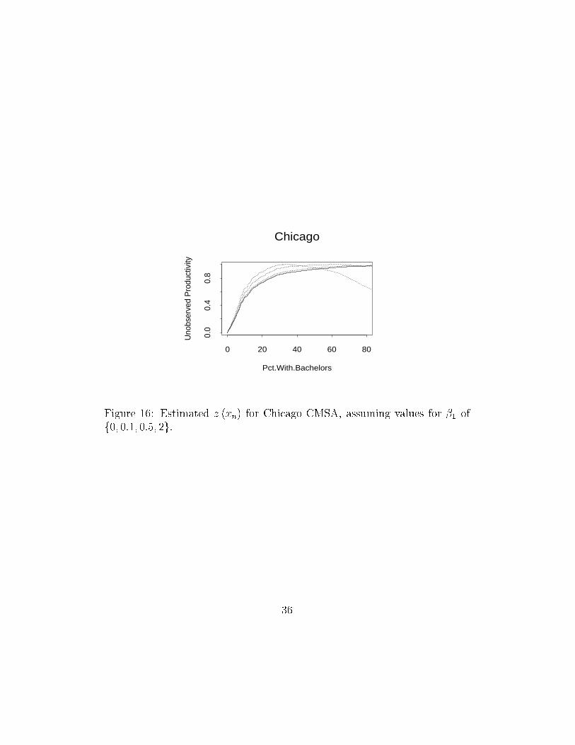
Figure 16 shows the estimated z (�xn) function for several values of�1. As the �gure shows, the estimates are not sensitive to alternativeassumptions about �1.
35
Chicago
Pct.With.Bachelors
Uno
bser
ved
Pro
duct
ivity
0 20 40 60 80
0.0
0.4
0.8
Figure 16: Estimated z (�xn) for Chicago CMSA, assuming values for �1 off0; 0:1; 0:5; 2g.
36