SNPdist appendix finaleffectivepopulation&sizewithin-host,&andthe&bottleneck&size.&Witha&knowntransmissionstructure&(for& instance,&within&a&household&

C. J. Worby et al. 2SI

File S1

1. Estimation of parameters

While the Geometric-‐Poisson distribution appears to approximate the distance distribution under simulation well, this

is under the assumption that several key parameters of interest are known – namely, the mutation rate, the

equilibrium effective population size within-‐host, and the bottleneck size. With a known transmission structure (for

instance, within a household (COWLING et al. 2010)), it is possible to estimate some of these quantities. We simulated

an outbreak and assumed that a set of 25 transmission pairs was observed. Figure S8 shows the likelihood of these

data under a range of values for mutation rate and effective population size. The estimate of the effective population

size is uncertain, since the data are less informative of this parameter; in the most extreme case, where coalescence

occurs immediately prior to the time of lineage divergence, the likelihood function depends only on the mutation

rate.

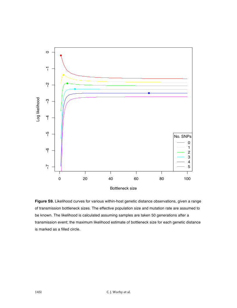
The bottleneck size can additionally be estimated. Observation of multiple genotypes shortly after a bottleneck event

suggests that the bottleneck must be large enough to allow diversity through; Figure S9 shows the likelihood of

observing different numbers of SNPs within host shortly after transmission, for a range of potential bottleneck sizes.

Again, such estimates are associated with very high levels of uncertainty, particularly for large bottleneck sizes.

However, it may be possible to test the hypothesis that the bottleneck size is strict, an assumption frequently made in

transmission network reconstruction methods.

2. Simulated outbreak

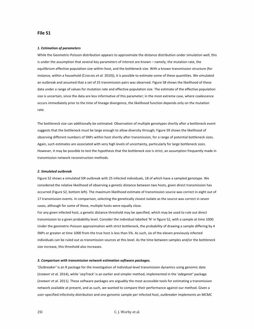
Figure S2 shows a simulated SIR outbreak with 25 infected individuals, 18 of which have a sampled genotype. We

considered the relative likelihood of observing a genetic distance between two hosts, given direct transmission has

occurred (Figure S2, bottom left). The maximum likelihood estimate of transmission source was correct in eight out of

17 transmission events. In comparison, selecting the genetically closest isolate as the source was correct in seven

cases, although for some of these, multiple hosts were equally close.

For any given infected host, a genetic distance threshold may be specified, which may be used to rule out direct

transmission to a given probability level. Consider the individual labelled ‘N’ in figure S2, with a sample at time 1000.

Under the geometric-‐Poisson approximation with strict bottleneck, the probability of drawing a sample differing by 4

SNPs or greater at time 1000 from the true host is less than 5%. As such, six of the eleven previously infected

individuals can be ruled out as transmission sources at this level. As the time between samples and/or the bottleneck

size increase, this threshold also increases.

3. Comparison with transmission network estimation software packages.

‘Outbreaker’ is an R package for the investigation of individual-‐level transmission dynamics using genomic data

(JOMBART et al. 2014), while ‘seqTrack’ is an earlier and simpler method, implemented in the ‘adegenet’ package

(JOMBART et al. 2011). These software packages are arguably the most accessible tools for estimating a transmission

network available at present, and as such, we wanted to compare their performance against our method. Given a

user-‐specified infectivity distribution and one genomic sample per infected host, outbreaker implements an MCMC


algorithm which estimates the posterior edge probabilities of the network, along with several parameters of interest,

including the mutation rate. Unlike our model, this approach therefore does not require infection times and mutation

rate to be known (and can also be used to detect importations into a population), however, it operates on a less

sophisticated model of within-‐host dynamics – mutations are assumed to be a feature of transmission, and an

infected host is adequately represented by a single sequenced pathogen isolate. seqTrack identifies the genetically

closest pathogen sample as the source, using the specified mutation rate to break ties. This approach also assumes

that each host is represented by one genomic sample.

We simulated outbreaks under various assumptions, and attempted to identify the transmission network using our

likelihood approach, as well as the outbreaker and seqTrack functions. While the outbreaker package can also be used

to simulate outbreaks, this is performed under the assumptions mentioned previously, so we instead simulated the

within-‐host pathogen dynamics explicitly, as described in Methods. We used the number of transmission routes to

compare the two methods. We ran outbreaker with no spatial model, and detection of importations suppressed.

Furthermore, we assumed a flat infectivity distribution. We emphasize that these approaches are not directly

comparable, since outbreaker and seqTrack accommodate unknown infection times, and outbreaker furthermore

estimates the mutation rate, giving our approach an advantage in this comparison. Results are presented in Table S2.

4. MRSA outbreak analysis

While the analysis provided in the main text provides estimates of transmission routes under plausible parameter

values found in the literature, there is a great deal of uncertainty surrounding true within-‐host pathogen population

dynamics, and as such, we repeated the analysis under a range of assumptions. The mutation rate used in the main

analysis was given in the paper describing this dataset; the mutation rate of MRSA has previously been estimated to

be higher ( 3×10−6 per nucleotide per year, equivalent to 5 ×10−4 per genome per generation (HARRIS et al.

2010; YOUNG et al. 2012)), so we repeated the analysis with this value. With this higher mutation rate, a larger range

of genetic distances are plausible, and as such, fewer routes were excluded at the 5% level. The HCW was a plausible

source for most patients on the ward, however, the genetic distance from patients 1 and 5 to the HCW were more

similar than would be expected, given this infection route. No patient to HCW transmission route could be excluded

at the 5% level.

Changing the effective population size had a limited effect on the estimated transmission route estimates. Values of

2000 and higher produced near identical posterior probabilities. Previous studies have estimated nasal carriage of S.

aureus to have an effective population size in the range of 50-‐4000 (YOUNG et al. 2012; GOLUBCHIK et al. 2013). We

experimented with an effective population size of 100, finding that five patient-‐HCW routes, and seven HCW-‐patient

routes could be excluded at the 5% level.

Varying the time at which the HCW became infected had an impact on posterior transmission probabilities. Moving

this value forward in time decreases the number of SNPs expected to accumulate by the time of observation. If the

HCW infection time was 164 days after the first case, the upper bound of the range provided by (HARRIS et al. 2013),

five patients remain temporally consistent with having become infected by the HCW. Two of these transmission

routes can be excluded at the 5% level.


We repeated our analysis using the pure Poisson model. In general, this distribution has a shorter right tail than the

geometric-‐Poisson distribution, and as such, can lead to more transmission routes being rejected at a given

probability level. With the same assumptions as in the main text, the HCW-‐patient routes were typically given a

higher posterior probability under the Poisson distribution, however, the most likely source of infection remained the

same for all individuals (Figure S5).

5. Conditional distributions

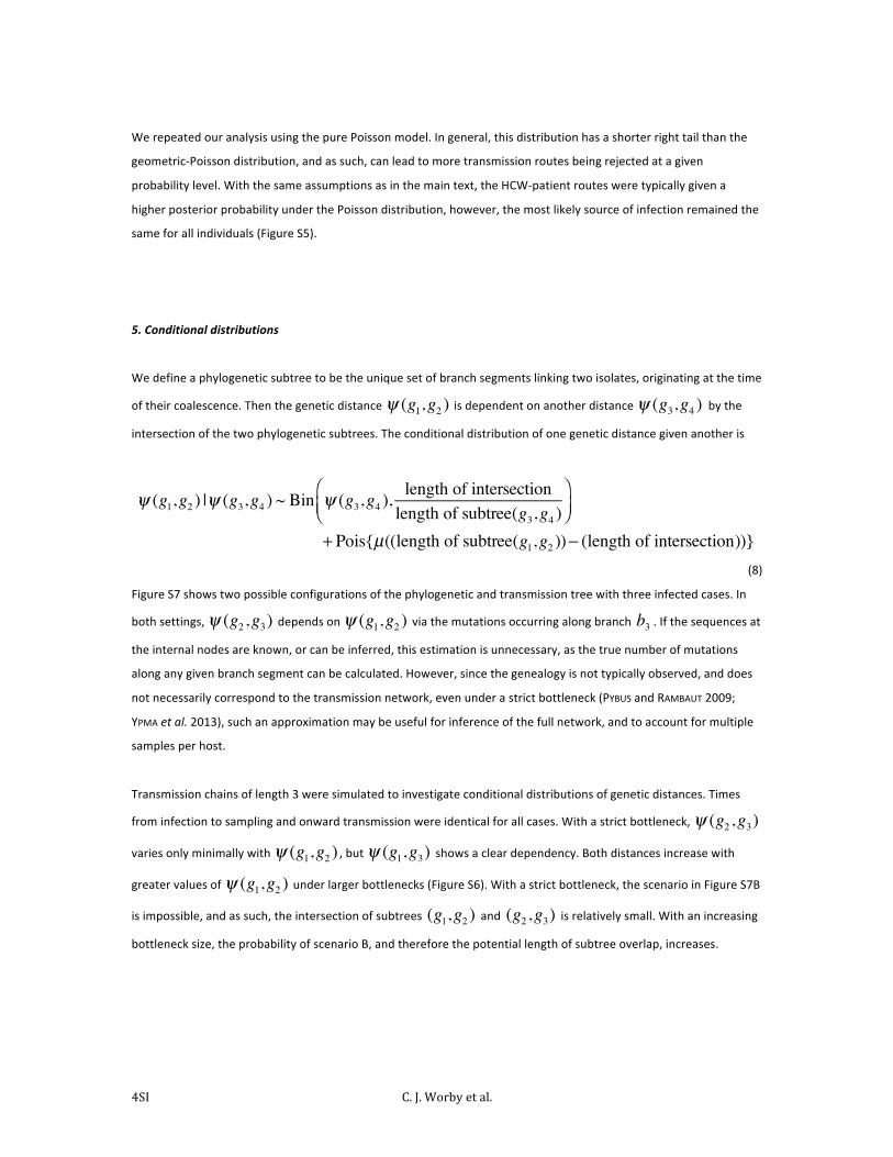
We define a phylogenetic subtree to be the unique set of branch segments linking two isolates, originating at the time

of their coalescence. Then the genetic distance ψ (g1,g2 ) is dependent on another distance ψ (g3,g4 ) by the intersection of the two phylogenetic subtrees. The conditional distribution of one genetic distance given another is

ψ (g1,g2 ) |ψ (g3,g4 ) ~ Bin ψ (g3,g4 ), length of intersectionlength of subtree(g3,g4 )

⎛⎝⎜

⎞⎠⎟

+ Pois{µ((length of subtree(g1,g2 ))− (length of intersection))}

(8)

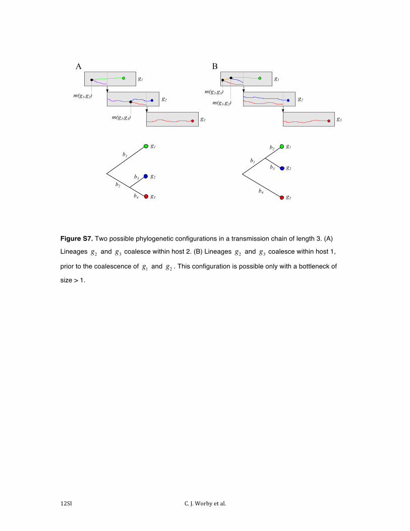
Figure S7 shows two possible configurations of the phylogenetic and transmission tree with three infected cases. In

both settings, ψ (g2,g3) depends on ψ (g1,g2 ) via the mutations occurring along branch b3 . If the sequences at the internal nodes are known, or can be inferred, this estimation is unnecessary, as the true number of mutations

along any given branch segment can be calculated. However, since the genealogy is not typically observed, and does

not necessarily correspond to the transmission network, even under a strict bottleneck (PYBUS and RAMBAUT 2009;

YPMA et al. 2013), such an approximation may be useful for inference of the full network, and to account for multiple

samples per host.

Transmission chains of length 3 were simulated to investigate conditional distributions of genetic distances. Times

from infection to sampling and onward transmission were identical for all cases. With a strict bottleneck, ψ (g2,g3)

varies only minimally with ψ (g1,g2 ) , but ψ (g1,g3) shows a clear dependency. Both distances increase with

greater values of ψ (g1,g2 ) under larger bottlenecks (Figure S6). With a strict bottleneck, the scenario in Figure S7B

is impossible, and as such, the intersection of subtrees (g1,g2 ) and (g2,g3) is relatively small. With an increasing

bottleneck size, the probability of scenario B, and therefore the potential length of subtree overlap, increases.


References

COWLING, B. J., K. H. CHAN, V. J. FANG, L. L. H. LAU, H. C. SO et al., 2010 Comparative

Epidemiology of Pandemic and Seasonal Influenza A in Households. New

England Journal of Medicine 362: 2175-‐2184.

GOLUBCHIK, T., E. M. BATTY, R. R. MILLER, H. FARR, B. C. YOUNG et al., 2013 Within-‐Host

Evolution of Staphylococcus aureus during Asymptomatic Carriage. PLoS One

8: e61319.

HARRIS, S. R., E. J. P. CARTWRIGHT, M. E. TÖRÖK, M. T. G. HOLDEN, N. M. BROWN et al., 2013

Whole-‐genome sequencing for analysis of an outbreak of meticillin-‐resistant

Staphylococcus aureus: a descriptive study. Lancet Infectious Diseases 13:

130-‐136.

HARRIS, S. R., E. J. FEIL, M. T. G. HOLDEN, M. A. QUAIL, E. K. NICKERSON et al., 2010

Evolution of MRSA during hospital transmission and intercontinental spread.

Science 327: 469-‐474.

JOMBART, T., A. CORI, X. DIDELOT, S. CAUCHEMEZ, C. FRASER et al., 2014 Bayesian

Reconstruction of Disease Outbreaks by Combining Epidemiologic and

Genomic Data. PLoS Computational Biology 10: e1003457.

JOMBART, T., R. M. EGGO, P. J. DODD and F. BALLOUX, 2011 Reconstructing disease

outbreaks from genetic data: a graph approach. Heredity 106: 383-‐390.

PYBUS, O. G., and A. RAMBAUT, 2009 Evolutionary analysis of the dynamics of viral

infectious disease. Nature Reviews Genetics 10: 540-‐550.

YOUNG, B. C., T. GOLUBCHIK, E. M. BATTY, R. FUNG, H. LARNER-‐SVENSSON et al., 2012

Evolutionary dynamics of Staphylococcus aureus during progression from

carriage to disease. PNAS 109: 4550-‐4555.

YPMA, R. J. F., W. M. VAN BALLEGOOIJEN and J. WALLINGA, 2013 Relating phylogenetic

trees to transmission trees of infectious disease outbreaks. Genetics 195:

1055-‐1062.


SI Figures

1ï��

��

��

ï��

��

��

2ï��

��

��

ï��

��

��

3ï��

��

��

ï��

��

��

�ï��

��

��

ï��

��

��

5ï��

��

��

ï��

��

��

6ï��

��

��

ï��

��

��

7ï��

��

��

ï��

��

��

8ï��

��

��

ï��

��

��

9ï��

��

��

1 5 ��ï��

��

��

1 5 �� 1 5 �� 1 5 �� 1 5 �� 1 5 �� 1 5 �� 1 5 �� 1 5 ��

��Bottleneck size

Und

eres

timat

e��1 ��

Und

eres

timat

e��1 ��

25 25 25 2525 25 25 2525

1 5 �� 1 5 �� 1 5 �� 1 5 �� 1 5 �� 1 5 �� 1 5 �� 1 5 �� 1 5 ��25 25 25 2525 25 25 2525

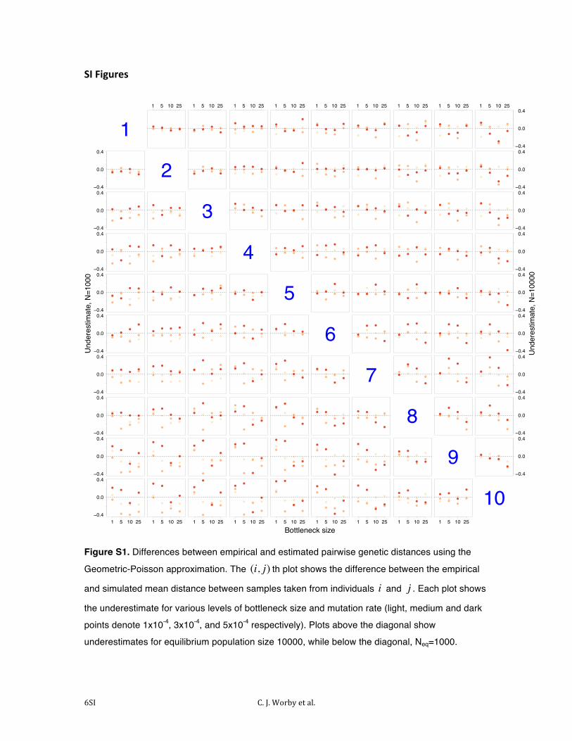
Figure S1. Differences between empirical and estimated pairwise genetic distances using the

Geometric-Poisson approximation. The (i, j) th plot shows the difference between the empirical

and simulated mean distance between samples taken from individuals i and j . Each plot shows

the underestimate for various levels of bottleneck size and mutation rate (light, medium and dark

points denote 1x10-4, 3x10-4, and 5x10-4 respectively). Plots above the diagonal show

underestimates for equilibrium population size 10000, while below the diagonal, Neq=1000.


0 500 1000 1500

Time

A

B

C

D

E

F

G

H

J

K

L

M

N

P

Q

R

S

T

U

V

W

X

Y

Z

Likelihood

Source

Recip

ien

t

A

B

C

D

E

G

H

J

K

L

M

N

P

R

S

V

W

Y

B C D E G H J K L M N P R S V W YA

Genetic distance

Source

Re

cip

ien

t7

8 3

8 7 8

5 4 5 3

6 5 6 4 1

5 4 5 3 0 1

7 2 3 7 4 5 4

6 1 2 6 3 4 3 1

7 6 7 5 2 3 2 6 5

7 6 7 5 2 3 2 6 5 0

7 6 7 5 2 3 2 6 5 0 0

7 2 3 7 4 5 4 2 1 6 6 6

6 5 6 4 1 2 1 5 4 3 3 3 5

6 1 2 6 3 4 3 1 0 5 5 5 1 4

7 6 7 3 2 3 2 6 5 4 4 4 6 3 5

7 2 3 7 4 5 4 2 1 6 6 6 2 5 1 6

6 1 2 6 3 4 3 1 0 5 5 5 1 4 0 5 1

A

B

C

D

E

G

H

J

K

L

M

N

P

R

S

V

W

Y

B C D E G H J K L M N P R S V W YA

Genetic Distance (No. SNPs)

0 1 2 3 4 5 6 7 8 9

Figure S2. A simulated outbreak. 24 individuals are infected in a simulated SIR outbreak, of

which 18 have sampled genotypes. Each individual has an infectious period shown as a gray bar,

with genotypes shown as colored circles, the color denoting the genetic distance from the first

sample (top). One randomly sampled genome for each individual is used to assess the likelihood

of direct transmission from each other sampled individual. The pairwise genetic distances are

shown (bottom right), with black boxes denoting the true source of infection, and gray boxes

denoting presence at the time of infection. The relative likelihood of direct transmission using the

geometric-Poisson approximation is shown for each pair (bottom left, green and red indicating

high and low relative likelihood respectively). Crosses indicate the maximum likelihood estimate,

while circles indicate the genetically closest isolate to each sample.


0.0 0.2 0.4 0.6 0.8 1.0

0.0

0.2

0.4

0.6

0.8

1.0

Estimated probability of infection route

Empi

rical

pro

babi

lity

of in

fect

ion

rout

e

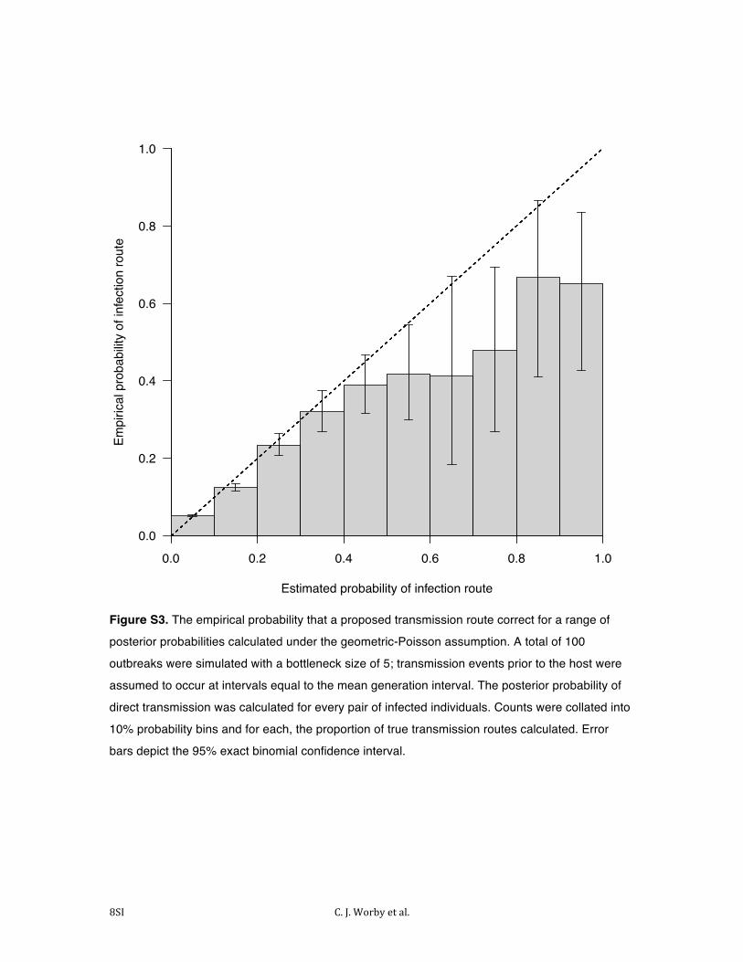
Figure S3. The empirical probability that a proposed transmission route correct for a range of

posterior probabilities calculated under the geometric-Poisson assumption. A total of 100

outbreaks were simulated with a bottleneck size of 5; transmission events prior to the host were

assumed to occur at intervals equal to the mean generation interval. The posterior probability of

direct transmission was calculated for every pair of infected individuals. Counts were collated into

10% probability bins and for each, the proportion of true transmission routes calculated. Error

bars depict the 95% exact binomial confidence interval.


11

12

1

2

3

13

5

4

6

8

7

14

15

109

2% [2%, 3%]

88% [8

3%, 9

1%]

H

11% [7%, 14%]

34% [21%, 39%]

66%

[61%

, 79%

]

71% [56%, 81%]

29% [19%, 44%]

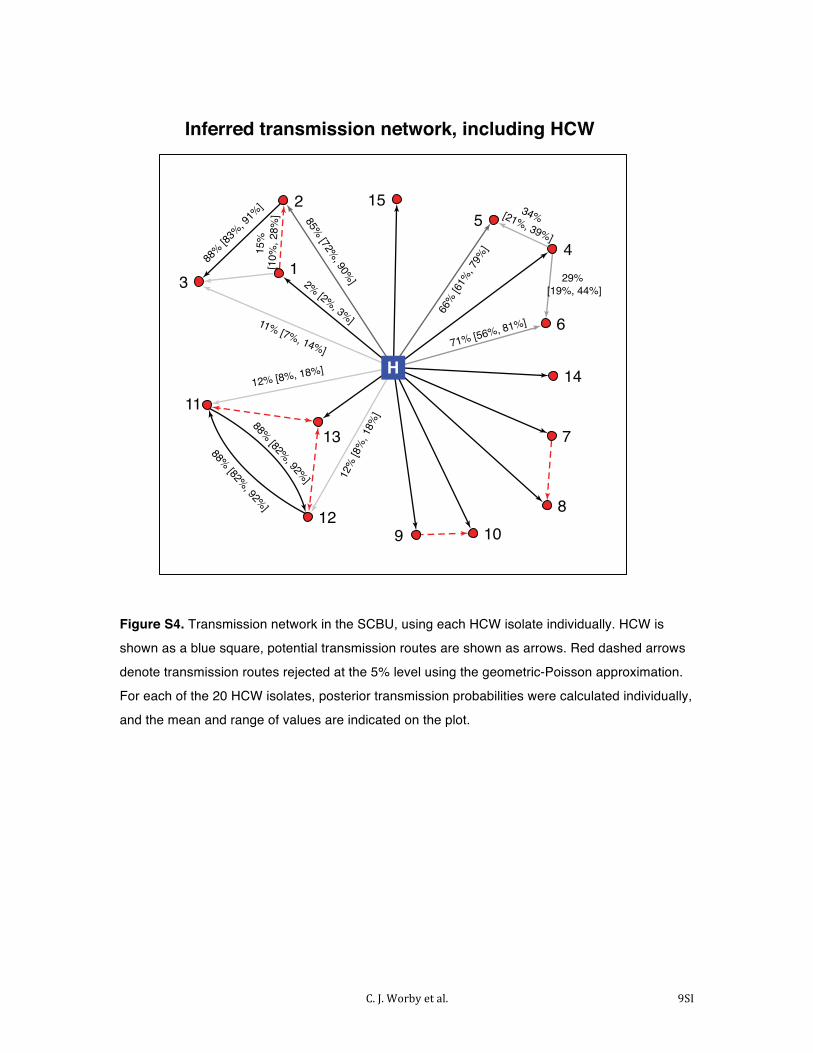
Inferred transmission network, including HCW

12% [8%, 18%]

88% [82%, 92%]85%

[72%, 90%

]

1

5%

[10%

, 28%

]

12%

[8%

, 18%

]

88% [82%, 92%]

Figure S4. Transmission network in the SCBU, using each HCW isolate individually. HCW is

shown as a blue square, potential transmission routes are shown as arrows. Red dashed arrows

denote transmission routes rejected at the 5% level using the geometric-Poisson approximation.

For each of the 20 HCW isolates, posterior transmission probabilities were calculated individually,

and the mean and range of values are indicated on the plot.


11

12

1

2

3

13

5

4

6

8

7

14

15

109

2%

88%

H

11%

27%

73%

80%

20%

Inferred transmission network, including HCW

18%

18%83%

83%

87%

12%

Figure S5. Transmission network in the SCBU, using the pure Poisson approximation. HCW is

shown as a blue square, potential transmission routes are shown as arrows. Red dashed arrows

denote transmission routes rejected at the 5% level using the Poisson approximation.


� � � � � ��

��

��

��

��

��

��

��

� �

�

� � � � � ��

��

��

��

��

��

��

��

��

��

��

��

��

� � � � � ��

��

��

��

��

��

��

��

� �

�

� � � � � ��

��

��

��

��

��

�

� � � � � ��

��

��

��

��

��

��

��

� �

�

� � � � � ��

��

��

��

��

��

��

� � � � � ��

��

��

��

��

��

��

!"#�

��

� �

�

� � � � � ��

��

��

��

��

��

��

!"#�

��

Figure S6. Simulated conditional distributions of genetic distances arising from a transmission

chain of length 3. Each row shows plots for ψ (g1,g3) and ψ (g2,g3) given various levels of

ψ (g1,g2 ) (denoted by different colors). Bottleneck size varies by row. Equilibrium size was set to

10000, and mutation rate µ = 3×10−4 .


��

��

��

��

��

��

� ��

��

��

��

��

��

��

��

��

��

��

��

��

��

��

��

Figure S7. Two possible phylogenetic configurations in a transmission chain of length 3. (A)

Lineages g2 and g3 coalesce within host 2. (B) Lineages g2 and g3 coalesce within host 1,

prior to the coalescence of g1 and g2 . This configuration is possible only with a bottleneck of

size > 1.


0 2000 4000 6000 8000 10000 120000.00

000.

0005

0.00

100.

0015

0.00

200.

0025

Effective population size

Mut

atio

n ra

te

Figure S8. Likelihood of observing 28 pairwise genetic distances between known transmission

pairs, given a range of values for the mutation rate and the effective population size. The dashed

lines indicate parameter values under which the data were simulated, and the geometric-Poisson

maximum likelihood value is marked. Maximum likelihood value calculated using the Nelder-Mead

method in the ‘optim’ function in R.


0 20 40 60 80 100

−7−6

−5−4

−3−2

−10

Bottleneck size

Log

likel

ihoo

d

●

●

●

●

●

No. SNPs012345

Figure S9. Likelihood curves for various within-host genetic distance observations, given a range

of transmission bottleneck sizes. The effective population size and mutation rate are assumed to

be known. The likelihood is calculated assuming samples are taken 50 generations after a

transmission event; the maximum likelihood estimate of bottleneck size for each genetic distance

is marked as a filled circle.


SI Tables

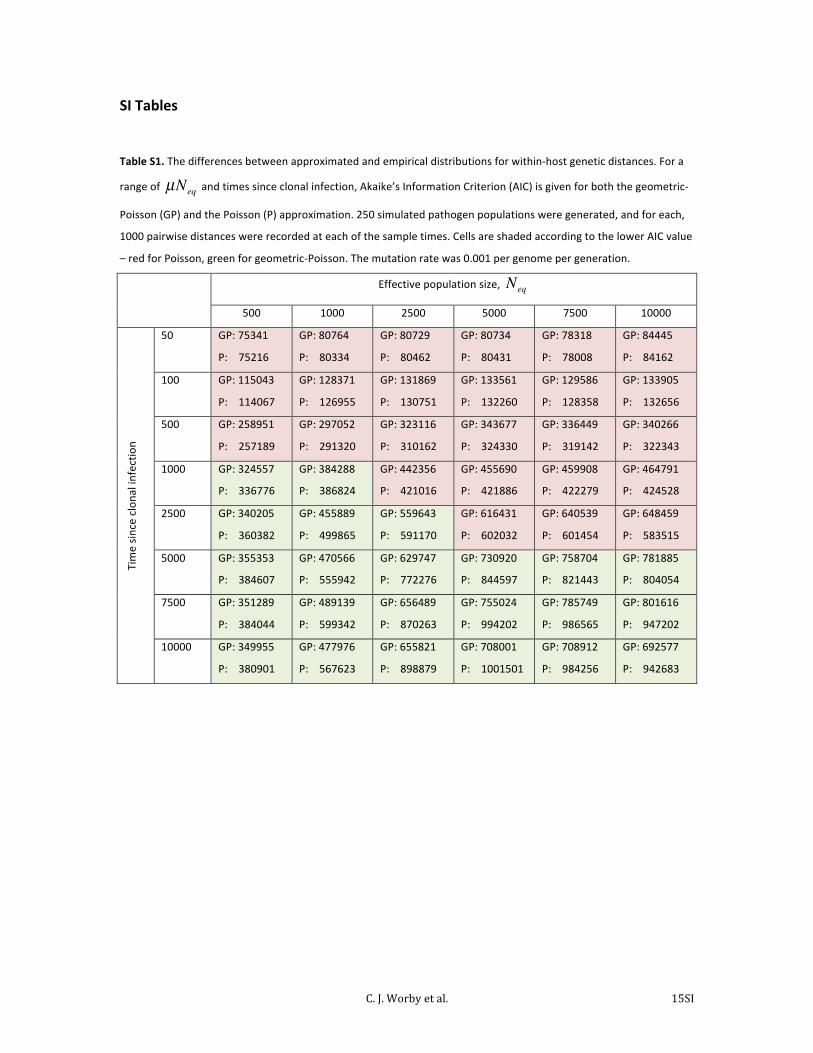
Table S1. The differences between approximated and empirical distributions for within-‐host genetic distances. For a

range of µNeq and times since clonal infection, Akaike’s Information Criterion (AIC) is given for both the geometric-‐

Poisson (GP) and the Poisson (P) approximation. 250 simulated pathogen populations were generated, and for each,

1000 pairwise distances were recorded at each of the sample times. Cells are shaded according to the lower AIC value

– red for Poisson, green for geometric-‐Poisson. The mutation rate was 0.001 per genome per generation.

Effective population size, Neq

500 1000 2500 5000 7500 10000

Time sin

ce clona

l infectio

n

50 GP: 75341

P: 75216

GP: 80764

P: 80334

GP: 80729

P: 80462

GP: 80734

P: 80431

GP: 78318

P: 78008

GP: 84445

P: 84162

100 GP: 115043

P: 114067

GP: 128371

P: 126955

GP: 131869

P: 130751

GP: 133561

P: 132260

GP: 129586

P: 128358

GP: 133905

P: 132656

500 GP: 258951

P: 257189

GP: 297052

P: 291320

GP: 323116

P: 310162

GP: 343677

P: 324330

GP: 336449

P: 319142

GP: 340266

P: 322343

1000 GP: 324557

P: 336776

GP: 384288

P: 386824

GP: 442356

P: 421016

GP: 455690

P: 421886

GP: 459908

P: 422279

GP: 464791

P: 424528

2500 GP: 340205

P: 360382

GP: 455889

P: 499865

GP: 559643

P: 591170

GP: 616431

P: 602032

GP: 640539

P: 601454

GP: 648459

P: 583515

5000 GP: 355353

P: 384607

GP: 470566

P: 555942

GP: 629747

P: 772276

GP: 730920

P: 844597

GP: 758704

P: 821443

GP: 781885

P: 804054

7500 GP: 351289

P: 384044

GP: 489139

P: 599342

GP: 656489

P: 870263

GP: 755024

P: 994202

GP: 785749

P: 986565

GP: 801616

P: 947202

10000 GP: 349955

P: 380901

GP: 477976

P: 567623

GP: 655821

P: 898879

GP: 708001

P: 1001501

GP: 708912

P: 984256

GP: 692577

P: 942683


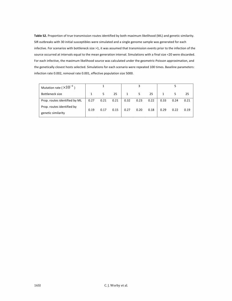
Table S2. Proportion of true transmission routes identified by both maximum likelihood (ML) and genetic similarity.

SIR outbreaks with 30 initial susceptibles were simulated and a single genome sample was generated for each

infective. For scenarios with bottleneck size >1, it was assumed that transmission events prior to the infection of the

source occurred at intervals equal to the mean generation interval. Simulations with a final size <20 were discarded.

For each infective, the maximum likelihood source was calculated under the geometric-‐Poisson approximation, and

the genetically closest hosts selected. Simulations for each scenario were repeated 100 times. Baseline parameters:

infection rate 0.002, removal rate 0.001, effective population size 5000.

Mutation rate (×10−4 ) 1 3 5

Bottleneck size 1 5 25 1 5 25 1 5 25

Prop. routes identified by ML 0.27 0.21 0.21 0.32 0.23 0.22 0.33 0.24 0.21

Prop. routes identified by

genetic similarity 0.19 0.17 0.15 0.27 0.20 0.18 0.29 0.22 0.19


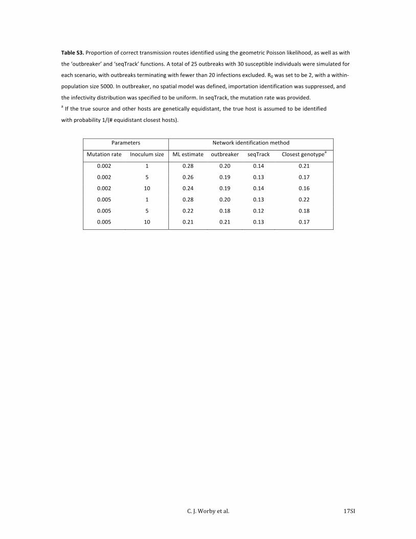
Table S3. Proportion of correct transmission routes identified using the geometric Poisson likelihood, as well as with

the ‘outbreaker’ and ‘seqTrack’ functions. A total of 25 outbreaks with 30 susceptible individuals were simulated for

each scenario, with outbreaks terminating with fewer than 20 infections excluded. R0 was set to be 2, with a within-‐

population size 5000. In outbreaker, no spatial model was defined, importation identification was suppressed, and

the infectivity distribution was specified to be uniform. In seqTrack, the mutation rate was provided. a If the true source and other hosts are genetically equidistant, the true host is assumed to be identified

with probability 1/(# equidistant closest hosts).

Parameters Network identification method

Mutation rate Inoculum size ML estimate outbreaker seqTrack Closest genotypea

0.002 1 0.28 0.20 0.14 0.21

0.002 5 0.26 0.19 0.13 0.17

0.002 10 0.24 0.19 0.14 0.16

0.005 1 0.28 0.20 0.13 0.22

0.005 5 0.22 0.18 0.12 0.18

0.005 10 0.21 0.21 0.13 0.17


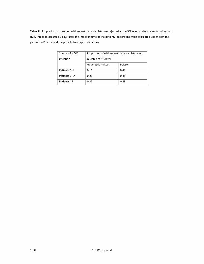
Table S4. Proportion of observed within-‐host pairwise distances rejected at the 5% level, under the assumption that

HCW infection occurred 2 days after the infection time of the patient. Proportions were calculated under both the

geometric-‐Poisson and the pure Poisson approximations.

Source of HCW

infection

Proportion of within-‐host pairwise distances

rejected at 5% level

Geometric-‐Poisson Poisson

Patients 1-‐6 0.16 0.48

Patients 7-‐14 0.25 0.48

Patients 15 0.35 0.48


Table S5. Transmission routes excluded at the 5% level under a range of scenarios.

Mutation

rate

Eff. Pop.

Size

HCW infection

time (relative to

first case)

HCW ruled out as

patient source

Patients ruled out

as HCW source

0.0002 3000 -‐23 NA 8,9,10,13,14

0.0005 3000 -‐23 NA NA

0.0002 10000 -‐23 NA 8,9,10,13,14

0.0002 100 -‐23 NA 8,9,10,13,14

0.0002 3000 164 1-‐10,13,14 –

0.0002 3000 -‐251 NA –

Documents

SNPdist appendix finaleffectivepopulation&sizewithin-host,&andthe&bottleneck&size.&Witha&knowntransmissionstructure&(for& instance,&within&a&household&