Embed Size (px)
Citation preview
SMUD’s Low Income Weatherization & Energy Management Pilot – Load Impact Evaluation
December 2014
Promoting residential energy and peak savings
for low‐income customers through enhanced
information, education, and smart thermostats
SMUD’s Low Income Weatherization & Energy Management Pilot –
Load Impact Evaluation

SMUD’s Low Income Weatherization & Energy Management Pilot – Load Impact Evaluation
PREPARED BY: Herter Energy Research Solutions, Inc. 2201 Francisco Drive, Suite 140‐120
El Dorado Hills, California www.HerterEnergy.com
Authors: Karen Herter, Ph.D. Yevgeniya Okuneva, Statistician
PREPARED FOR: Sacramento Municipal Utility District Sacramento, California
Program Manager: Lupe Strickland
Project Manager: Bobbie Harris
Evaluation Coordinator: Nanako Wong
SMUD Contract No: 4500071792
This material is based upon work supported by the Department of Energy under Award Number OE000214.
© 2014 Herter Energy Research Solutions, Inc.
Suggested Citation: Herter, Karen, and Yevgeniya Okuneva. 2014. SMUD’s Low Income Weatherization & Energy Management Pilot – Load Impact Evaluation. Prepared by Herter Energy Research Solutions for the Sacramento Municipal Utility District.

SMUD’s Low Income Weatherization & Energy Management Pilot – Load Impact Evaluation i
Acknowledgement: This material is based upon work supported by the Department of
Energy under Award Number OE000214.
Disclaimer: This report was prepared as an account of work sponsored by an agency of
the United States Government. Neither the United States Government nor any agency
thereof, nor any of their employees, makes any warranty, express or implied, or
assumes any legal liability or responsibility for the accuracy, completeness, or usefulness
of any information, apparatus, product, or process disclosed, or represents that its use
would not infringe privately owned rights. Reference herein to any specific commercial
product, process, or service by trade name, trademark, manufacturer, or otherwise does
not necessarily constitute or imply its endorsement, recommendation, or favoring by
the United States Government or any agency thereof. The views and opinions of
authors expressed herein do not necessarily state or reflect those of the United States
Government or any agency thereof.

SMUD’s Low Income Weatherization & Energy Management Pilot – Load Impact Evaluation ii
CONTENTS
EXECUTIVE SUMMARY 1
1. INTRODUCTION 3
PROBLEM STATEMENT 3
STUDY OVERVIEW 3
IMPLEMENTATION 5
2. DATA 10
EVALUATION PERIOD 10
SAMPLE POPULATION 10
POTENTIAL SOURCES OF BIAS 13
LOAD DATA 16
TEMPERATURE DATA 21
3. ANALYSIS AND RESULTS 23
APPROACH 23
NULL HYPOTHESES 25
LOAD IMPACTS OF THE AUDIT ONLY 26
TREATMENT EFFECTS – YDT, IHD, AND NEST 27
4. CONCLUSIONS 33
REFERENCES 34
5. APPENDICES 35
APPENDIX A. SUMMER WEEKDAY LOAD MODEL 35
APPENDIX B. SEASONAL LOAD MODEL 62
APPENDIX C. BILL MODEL FIT 73
APPENDIX D. DEMOGRAPHIC DATA SUMMARY 74
SMUD’s Low Income Weatherization & Energy Management Pilot – Load Impact Evaluation iii
FIGURES FIGURE 1. PEAK IMPACTS RELATIVE TO THE AUDIT GROUP ........................................................................................... 1 FIGURE 2. ANNUAL AND SEASONAL ENERGY IMPACTS RELATIVE TO THE AUDIT GROUP ....................................................... 2 FIGURE 3. BILL IMPACTS ....................................................................................................................................... 2 FIGURE 4. YESTERDAY’S DATA TODAY ONLINE: MY HOURLY ELECTRICITY USE ................................................................ 7 FIGURE 5. THE POWERTAB IN‐HOME DISPLAY .......................................................................................................... 7 FIGURE 6. THE NEST THERMOSTAT AND SMARTPHONE APP ......................................................................................... 8 FIGURE 7. MAP OF PARTICIPANTS, BY TREATMENT ................................................................................................... 12 FIGURE 8. AVERAGE SUMMER LOADS 2011 ............................................................................................................ 16 FIGURE 9. AVERAGE WINTER LOADS 2011‐2012 .................................................................................................... 16 FIGURE 10. PRETREATMENT AVERAGE ENERGY USE .................................................................................................. 17 FIGURE 11. PRETREATMENT AVERAGE PEAK DEMAND ............................................................................................... 18 FIGURE 12. PRETREATMENT AUGUST ENERGY USE, GENERAL AND INVITED POPULATIONS ................................................ 19 FIGURE 13. SUMMER PEAK DEMAND, INVITED POPULATION ...................................................................................... 20 FIGURE 14. WEATHER STATIONS USED FOR LOAD IMPACT EVALUATION ........................................................................ 21 FIGURE 15. AVERAGE HOURLY TEMPERATURE READINGS, SUMMER 2013 .................................................................... 22 FIGURE 16. BOXPLOTS OF MAXIMUM DAILY TEMPERATURE READINGS, SUMMER 2013 ................................................... 22 FIGURE 17. ACTUAL VS. MODELED STANDARD RATE BILLS, WINTER 2013 ..................................................................... 26 FIGURE 18. SUMMER WEEKDAY IMPACTS, RELATIVE TO THE SURVEYED CONTROL GROUP ................................................. 28 FIGURE 19. AVERAGE SUMMER ENERGY IMPACTS, RELATIVE TO THE AUDIT GROUP ......................................................... 30 FIGURE 20. BOXPLOT OF AVERAGE SUMMER BILL IMPACTS ($/MONTH) ....................................................................... 30 FIGURE 21. AVERAGE WINTER ENERGY IMPACTS, RELATIVE TO THE SURVEYED CONTROL GROUP ........................................ 31 FIGURE 22. BOXPLOT OF AVERAGE WINTER BILL IMPACTS ($/MONTH) ......................................................................... 31 FIGURE 23. ACTUAL AND MODELED SUMMER LOADS, YDT ........................................................................................ 36 FIGURE 24. ACTUAL AND MODELED SUMMER LOADS, IHD ........................................................................................ 36 FIGURE 25. ACTUAL AND MODELED SUMMER LOADS, NEST ....................................................................................... 36 FIGURE 26. ACTUAL AND MODELED SUMMER LOADS, AUDIT ...................................................................................... 37 FIGURE 27.SCATTER PLOT OF NORMALIZED RESIDUALS VERSUS FITTED VALUES FOR PRE PEAK MODEL ................................ 38 FIGURE 28.NORMAL PLOT OF ESTIMATED RANDOM EFFECTS (CUSTOMER LEVEL), PRE PEAK MODEL .................................. 38 FIGURE 29.NORMAL PLOT OF ESTIMATED RANDOM EFFECTS (DAY LEVEL), PRE PEAK MODEL ............................................ 39 FIGURE 30.NORMAL PLOT OF RESIDUALS, PRE PEAK MODEL ...................................................................................... 39 FIGURE 31.HISTOGRAM OF NORMALIZED RESIDUALS, PRE PEAK MODEL ...................................................................... 40 FIGURE 32.SCATTER PLOT MATRIX OF PEARSON AND NORMALIZED RESIDUALS, PRE PEAK MODEL .................................... 41 FIGURE 33.SCATTER PLOT OF NORMALIZED RESIDUALS VERSUS FITTED VALUES FOR PEAK MODEL ..................................... 42 FIGURE 34.NORMAL PLOT OF ESTIMATED RANDOM EFFECTS (CUSTOMER LEVEL), PEAK MODEL ....................................... 42 FIGURE 35.NORMAL PLOT OF ESTIMATED RANDOM EFFECTS (DAY LEVEL), PEAK MODEL ................................................. 43 FIGURE 36.NORMAL PLOT OF RESIDUALS, PEAK MODEL ........................................................................................... 43 FIGURE 37.HISTOGRAM OF NORMALIZED RESIDUALS, PEAK MODEL ............................................................................ 44 FIGURE 38.SCATTER PLOT MATRIX OF PEARSON AND NORMALIZED RESIDUALS, PEAK MODEL .......................................... 45 FIGURE 39.SCATTER PLOT OF NORMALIZED RESIDUALS VERSUS FITTED VALUES FOR POST PEAK MODEL .............................. 46 FIGURE 40.NORMAL PLOT OF ESTIMATED RANDOM EFFECTS (CUSTOMER LEVEL), POST PEAK MODEL ................................ 46 FIGURE 41.NORMAL PLOT OF ESTIMATED RANDOM EFFECTS (DAY LEVEL), POST PEAK MODEL ......................................... 47 FIGURE 42.NORMAL PLOT OF RESIDUALS, POST PEAK MODEL ................................................................................... 47
SMUD’s Low Income Weatherization & Energy Management Pilot – Load Impact Evaluation iv
FIGURE 43.HISTOGRAM OF NORMALIZED RESIDUALS, POST PEAK MODEL .................................................................... 48 FIGURE 44.SCATTER PLOT MATRIX OF PEARSON AND NORMALIZED RESIDUALS, POST PEAK MODEL .................................. 49 FIGURE 45. ACTUAL AND MODELED LOADS, SEASONAL MODEL ................................................................................... 63 FIGURE 46.SCATTER PLOT OF NORMALIZED RESIDUALS VERSUS FITTED VALUES FOR SEASONAL MODEL ................................ 64 FIGURE 47.NORMAL PLOTS OF ESTIMATED RANDOM EFFECTS, SEASONAL MODEL ........................................................... 64 FIGURE 48.SCATTER PLOT MATRIX OF RANDOM EFFECTS, SEASONAL MODEL .................................................................. 65 FIGURE 49.NORMAL PLOT OF RESIDUALS, SEASONAL MODEL ...................................................................................... 65 FIGURE 50.EMPIRICAL AUTOCORRELATION FUNCTION CORRESPONDING TO NORMALIZED RESIDUALS, SEASONAL MODEL ........ 66 FIGURE 51. ACTUAL VS. MODELED STANDARD LOW‐INCOME RATE BILLS, SUMMER 2013 ................................................ 73 FIGURE 52. ACTUAL VS. MODELED STANDARD RATE BILLS, WINTER 2013 ..................................................................... 73 FIGURE 53. CORRELATION MATRIX: ANNUAL ENERGY IMPACT AND DEMOGRAPHICS, YDT ............................................... 74 FIGURE 54. CORRELATION MATRIX: ANNUAL ENERGY IMPACT AND DEMOGRAPHICS, IHD ................................................ 75 FIGURE 55. CORRELATION MATRIX: ANNUAL ENERGY IMPACT AND DEMOGRAPHICS, NEST............................................... 76 FIGURE 56. CORRELATION MATRIX: ANNUAL ENERGY IMPACT AND DEMOGRAPHICS, AUDIT ............................................. 77
SMUD’s Low Income Weatherization & Energy Management Pilot – Load Impact Evaluation v
TABLES TABLE 1. ENERGY INSIGHTS WEATHERIZATION STUDY SCHEDULE .................................................................................. 5 TABLE 2. SMUD’S 2013 ENERGY ASSISTANCE PROGRAM RATE PRICING ($/KWH) .......................................................... 6 TABLE 3. TREATMENT GROUP MEASURES ................................................................................................................. 6 TABLE 4. EVALUATION PERIOD START AND END DATES .............................................................................................. 10 TABLE 5. FINAL SAMPLE SIZES .............................................................................................................................. 11 TABLE 6. CONTROL GROUP LOAD IMPACT COMPARISON ............................................................................................ 15 TABLE 7. PRETREATMENT AVERAGE ENERGY USE COMPARISONS (P‐VALUES) ................................................................. 17 TABLE 8. PRETREATMENT AVERAGE PEAK DEMAND COMPARISONS (P‐VALUES) .............................................................. 18 TABLE 9. PRETREATMENT AUGUST ENERGY USE COMPARISON, GENERAL AND INVITED POPULATIONS ................................. 19 TABLE 10. SUMMER PEAK DEMAND COMPARISON, PARTICIPANTS AND INVITED ............................................................. 20 TABLE 11. AVERAGE SUMMER WEEKDAY IMPACTS FOR THE AUDIT GROUP .................................................................... 26 TABLE 12. AVERAGE ENERGY IMPACTS FOR THE AUDIT GROUP ................................................................................... 27 TABLE 13. SUMMER WEEKDAY DEMAND IMPACTS, RELATIVE TO THE AUDIT GROUP ........................................................ 28 TABLE 14. AVERAGE ENERGY IMPACTS OF TREATMENTS, RELATIVE TO THE AUDIT GROUP ................................................. 29 TABLE 15. AVERAGE MONTHLY BILL IMPACTS OF TREATMENTS, RELATIVE TO THE AUDIT GROUP ........................................ 29 TABLE 16. CORRELATIONS WITH ANNUAL ENERGY IMPACT (PEARSON’S R) .................................................................... 32 TABLE 17.SUMMARY OF RESIDUALS, PRE PEAK MODEL............................................................................................. 40 TABLE 18.SUMMARY OF RESIDUALS, PEAK MODEL .................................................................................................. 44 TABLE 19.SUMMARY OF RESIDUALS, POST PEAK MODEL .......................................................................................... 48 TABLE 20.MODEL COMPARISON, PRE PEAK MODEL ................................................................................................ 51 TABLE 21.MODEL COMPARISON, PEAK MODEL ...................................................................................................... 51 TABLE 22.MODEL COMPARISON, POST PEAK MODEL .............................................................................................. 51 TABLE 23.F‐TESTS FOR VARIABLES IN THE MODEL, PRE PEAK MODEL ........................................................................... 52 TABLE 24. F‐TESTS FOR VARIABLES IN THE MODEL, PEAK MODEL ............................................................................... 52 TABLE 25. F‐TESTS FOR VARIABLES IN THE MODEL, POST PEAK MODEL ........................................................................ 52 TABLE 26.CONDITIONAL R2 FOR PRE PEAK, PEAK, AND POST PEAK MODELS ............................................................... 53 TABLE 27. MODEL COEFFICIENTS, PRE PEAK MODEL ................................................................................................ 53 TABLE 28. MODEL COEFFICIENTS, PEAK MODEL ..................................................................................................... 55 TABLE 29. MODEL COEFFICIENTS, POST PEAK MODEL ............................................................................................. 57 TABLE 30. VARIANCE COVARIANCE MATRIX, PRE PEAK MODEL ................................................................................... 59 TABLE 31. VARIANCE COVARIANCE MATRIX, PEAK MODEL ........................................................................................ 59 TABLE 32. VARIANCE COVARIANCE MATRIX, POST PEAK MODEL ................................................................................. 59 TABLE 33.SUMMER WEEKDAY IMPACTS FOR AUDIT, RELATIVE TO SURVEY CONTROL GROUP ............................................. 60 TABLE 34. SUMMER WEEKDAY IMPACTS FOR TREATMENTS, RELATIVE TO THE AUDIT ONLY GROUP .................................... 60 TABLE 35.SUMMER WEEKDAY IMPACTS, BETWEEN‐TREATMENT COMPARISONS ............................................................. 61 TABLE 36.SUMMARY OF RESIDUALS, SEASONAL MODEL ............................................................................................ 66 TABLE 37.MODEL COMPARISON, SEASONAL MODEL ................................................................................................ 68 TABLE 38. F‐TESTS FOR VARIABLES IN THE MODEL, SEASONAL MODEL .......................................................................... 68 TABLE 39.MODEL COEFFICIENTS, SEASONAL MODEL ................................................................................................ 69 TABLE 40.VARIANCE COVARIANCE MATRIX, SEASONAL MODEL ................................................................................... 70 TABLE 41. ENERGY IMPACTS FOR AUDIT, RELATIVE TO THE SURVEYED CONTROL GROUP ................................................... 71 TABLE 42. ENERGY IMPACTS FOR TREATMENTS, RELATIVE TO AUDIT ............................................................................ 71
SMUD’s Low Income Weatherization & Energy Management Pilot – Load Impact Evaluation vi
TABLE 43. ENERGY IMPACTS, BETWEEN‐TREATMENT COMPARISONS ............................................................................ 72 TABLE 44.SUMMARY OF RESPONSES, WHO PAYS THE ELECTRICITY BILL ......................................................................... 78 TABLE 45.MEAN DIFFERENCES ANALYSIS FOR PARTICIPANT AGE .................................................................................. 78 TABLE 46.SUMMARY OF RESPONSES, PARTICIPANT AGE ............................................................................................ 78 TABLE 47.SUMMARY OF RESPONSES, GENDER ......................................................................................................... 79 TABLE 48.SUMMARY OF RESPONSES, HOUSEHOLD OCCUPANTS .................................................................................. 79 TABLE 49.SUMMARY OF RESPONSES, HOUSEHOLD OCCUPANTS UNDER THE AGE OF 18 ................................................... 80 TABLE 50.SUMMARY OF RESPONSES, HOUSEHOLD OCCUPANTS DURING THE 4‐7 PM PEAK ............................................... 80 TABLE 51.SUMMARY OF RESPONSES, OWN/RENT .................................................................................................... 81 TABLE 52.SUMMARY OF RESPONSES, ETHNIC GROUP ................................................................................................ 81 TABLE 53.SUMMARY OF RESPONSES, PRIMARY LANGUAGE SPOKEN AT HOME ................................................................ 82 TABLE 54.SUMMARY OF RESPONSES, PARTICIPANT EDUCATION .................................................................................. 83 TABLE 55.MEAN DIFFERENCES ANALYSIS FOR PARTICIPANT EDUCATION ........................................................................ 83 TABLE 56.NUMBER OF PARTICIPANTS WITH NO RESPONSE, DAYLIGHT SUMMER HOURS THERMOSTAT SETTINGS ................... 84 TABLE 57.MEAN DIFFERENCES ANALYSIS FOR SUMMER DAYLIGHT HOURS THERMOSTAT SETTINGS ..................................... 84 TABLE 58.NUMBER OF PARTICIPANTS WITH NO RESPONSE, SUMMER NIGHT TIME HOURS THERMOSTAT SETTINGS ................. 84 TABLE 59.MEAN DIFFERENCES ANALYSIS FOR SUMMER NIGHT TIME HOURS THERMOSTAT SETTINGS ................................... 85 TABLE 60.NUMBER OF PARTICIPANTS WITH NO RESPONSE, WINTER DAYLIGHT HOURS THERMOSTAT SETTINGS ..................... 85 TABLE 61.MEAN DIFFERENCES ANALYSIS FOR WINTER DAYLIGHT HOURS THERMOSTAT SETTINGS ....................................... 85 TABLE 62.NUMBER OF PARTICIPANTS WITH NO RESPONSE, WINTER NIGHT TIME HOURS THERMOSTAT SETTINGS .................. 86 TABLE 63.MEAN DIFFERENCES ANALYSIS FOR WINTER NIGHT TIME HOURS THERMOSTAT SETTINGS .................................... 86 TABLE 64.SUMMARY OF RESPONSES, DWELLING TYPE ............................................................................................... 86 TABLE 65.SUMMARY OF RESPONSES, OWN/RENT .................................................................................................... 87 TABLE 66.SUMMARY OF RESPONSES, RATE ............................................................................................................. 87 TABLE 67.SUMMARY OF RESPONSES, WHO PAYS BILLS .............................................................................................. 87
SMUD’s Low Income Weatherization & Energy Management Pilot – Load Impact Evaluation
1
EXECUTIVE SUMMARY This study investigates whether the provision of measures beyond SMUD’s standard Low‐
Income Weatherization program – smart thermostats (Nest), in‐home energy displays (IHD),
and training on web‐based hourly electricity use summaries, known internally at SMUD as
Yesterday’s Data Today (YDT) – might help low‐income customers further reduce their energy
use and peak loads. To this end, SMUD offered and implemented these three treatment
measures in about 400 homes on the low‐income Energy Assistance Program Rate (EAPR). All
three treatment groups received SMUD’s standard Low‐Income Weatherization Audit.
A fourth group receiving only the audit (Audit) was used as the control for the load impact
analysis. On average, participants in the Audit group saved a statistically significant 490 kWh
annually – 310 kWh in the summer and 170 kWh in the winter – for a total of 4.8% of their
annual energy use. During the summer peak hours of 4 to 7 p.m., participants in the Audit
group saved a statistically significant 220 watts on average, or 9.2% of their peak load.
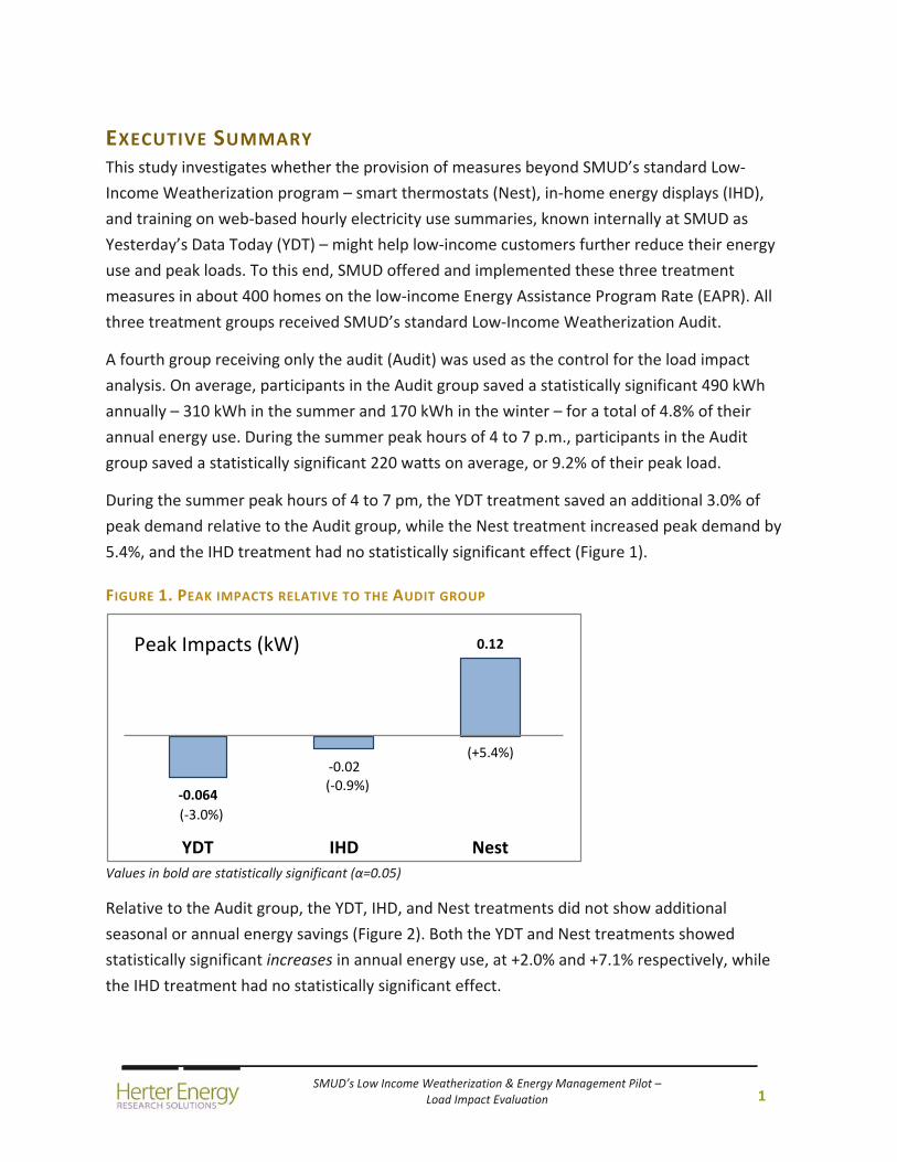
During the summer peak hours of 4 to 7 pm, the YDT treatment saved an additional 3.0% of
peak demand relative to the Audit group, while the Nest treatment increased peak demand by
5.4%, and the IHD treatment had no statistically significant effect (Figure 1).
FIGURE 1. PEAK IMPACTS RELATIVE TO THE AUDIT GROUP
Values in bold are statistically significant (α=0.05)
Relative to the Audit group, the YDT, IHD, and Nest treatments did not show additional
seasonal or annual energy savings (Figure 2). Both the YDT and Nest treatments showed
statistically significant increases in annual energy use, at +2.0% and +7.1% respectively, while
the IHD treatment had no statistically significant effect.
‐0.064
‐0.02
0.12
YDT
IHD
Nest
Peak Impacts (kW)
(‐3.0%)
(‐0.9%)
(+5.4%)

SMUD’s Low Income Weatherization & Energy Management Pilot – Load Impact Evaluation
2
FIGURE 2. ANNUAL AND SEASONAL ENERGY IMPACTS RELATIVE TO THE AUDIT GROUP
Values in bold are statistically significant (α=0.05)
Similarly, the treatments of interest did not reduce electricity bills relative to the Audit group
(Figure 3). Statistically significant bill increases were evident in the Nest group.
FIGURE 3. BILL IMPACTS
Values in bold are statistically significant (α=0.05)
In summary, the results of this load impact evaluation indicate that SMUD’s Low‐income
Weatherization Audit effectively reduced energy use and bills for low‐income customers.
Beyond the Audit, however, training on SMUD’s Yesterday’s Data Today website (YDT), the
provision of a real‐time energy display (IHD), and the installation of a Nest Learning thermostat
(Nest) were not effective in reducing energy use or bills further. The 7.1% annual energy
increase for the low‐income customers provided with a Nest thermostat suggests that future
programs that involve the Nest, or perhaps any other smart thermostat, might consider the
low‐income population separately from the standard population.
41 32
228 162
29
449
203
61
677
YDT
IHD
Nest
Energy Impacts (kWh) Summer Winter Annual
(0.8%) (2.8%) (2.0%) (0.6%) (0.6%) (0.6%) (5.8%) (8.0%) (7.1%)
$2 $0
$22 $23
$5
$47
$25
$5
$69
YDT IHD Nest
Bill Impacts Summer Winter Annual
(0.7%) (5.8%) (3.6%) (0.0%) (1.3%) (0.8%) (7.7%) (12.6%) (10.5%)
SMUD’s Low Income Weatherization & Energy Management Pilot – Load Impact Evaluation
3
1. INTRODUCTION
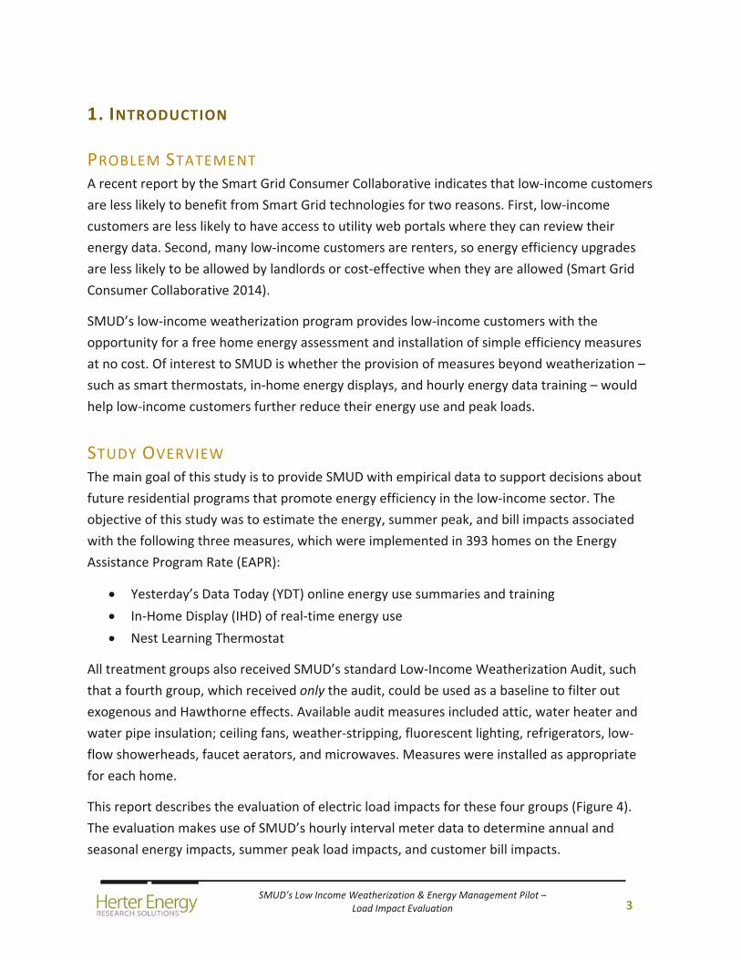
PROBLEM STATEMENT A recent report by the Smart Grid Consumer Collaborative indicates that low‐income customers
are less likely to benefit from Smart Grid technologies for two reasons. First, low‐income
customers are less likely to have access to utility web portals where they can review their
energy data. Second, many low‐income customers are renters, so energy efficiency upgrades
are less likely to be allowed by landlords or cost‐effective when they are allowed (Smart Grid
Consumer Collaborative 2014).
SMUD’s low‐income weatherization program provides low‐income customers with the
opportunity for a free home energy assessment and installation of simple efficiency measures
at no cost. Of interest to SMUD is whether the provision of measures beyond weatherization –
such as smart thermostats, in‐home energy displays, and hourly energy data training – would
help low‐income customers further reduce their energy use and peak loads.
STUDY OVERVIEW The main goal of this study is to provide SMUD with empirical data to support decisions about
future residential programs that promote energy efficiency in the low‐income sector. The
objective of this study was to estimate the energy, summer peak, and bill impacts associated
with the following three measures, which were implemented in 393 homes on the Energy
Assistance Program Rate (EAPR):
Yesterday’s Data Today (YDT) online energy use summaries and training
In‐Home Display (IHD) of real‐time energy use
Nest Learning Thermostat
All treatment groups also received SMUD’s standard Low‐Income Weatherization Audit, such
that a fourth group, which received only the audit, could be used as a baseline to filter out
exogenous and Hawthorne effects. Available audit measures included attic, water heater and
water pipe insulation; ceiling fans, weather‐stripping, fluorescent lighting, refrigerators, low‐
flow showerheads, faucet aerators, and microwaves. Measures were installed as appropriate
for each home.
This report describes the evaluation of electric load impacts for these four groups (Figure 4).
The evaluation makes use of SMUD’s hourly interval meter data to determine annual and
seasonal energy impacts, summer peak load impacts, and customer bill impacts.
SMUD’s Low Income Weatherization & Energy Management Pilot – Load Impact Evaluation
4
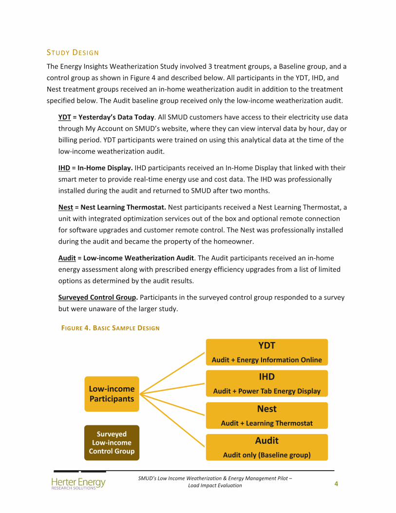
STUDY DESIGN
The Energy Insights Weatherization Study involved 3 treatment groups, a Baseline group, and a
control group as shown in Figure 4 and described below. All participants in the YDT, IHD, and
Nest treatment groups received an in‐home weatherization audit in addition to the treatment
specified below. The Audit baseline group received only the low‐income weatherization audit.
YDT = Yesterday’s Data Today. All SMUD customers have access to their electricity use data
through My Account on SMUD’s website, where they can view interval data by hour, day or
billing period. YDT participants were trained on using this analytical data at the time of the
low‐income weatherization audit.
IHD = In‐Home Display. IHD participants received an In‐Home Display that linked with their
smart meter to provide real‐time energy use and cost data. The IHD was professionally
installed during the audit and returned to SMUD after two months.
Nest = Nest Learning Thermostat. Nest participants received a Nest Learning Thermostat, a
unit with integrated optimization services out of the box and optional remote connection
for software upgrades and customer remote control. The Nest was professionally installed
during the audit and became the property of the homeowner.
Audit = Low‐income Weatherization Audit. The Audit participants received an in‐home
energy assessment along with prescribed energy efficiency upgrades from a list of limited
options as determined by the audit results.
Surveyed Control Group. Participants in the surveyed control group responded to a survey
but were unaware of the larger study.
FIGURE 4. BASIC SAMPLE DESIGN
Low‐income Participants
Audit
Audit only (Baseline group)
YDT
Audit + Energy Information Online
IHD
Audit + Power Tab Energy Display
Nest
Audit + Learning Thermostat
Surveyed Low‐income Control Group
SMUD’s Low Income Weatherization & Energy Management Pilot – Load Impact Evaluation
5
EVALUATION PERIOD
The pretreatment period for the Energy Insights Weatherization Study spans from August 2011
to May 2012, while the treatment period starts in February 2013 and ends in January 2014. For
the analysis, the summer months of August and September 2011 are used to construct the
baseline loads to which the June through September 2013 loads are compared. Loads from the
summer of 2012 could not be used because they were affected by recruitment efforts.
While the months of June and July are missing from the pretreatment period due to a lack of
meter data prior to August 2011, this is not expected to have a substantial effect on final results
because they are corrected for temperature effects; i.e. the baseline loads estimated from
pretreatment data are adjusted to reflect outdoor temperatures during the treatment period.
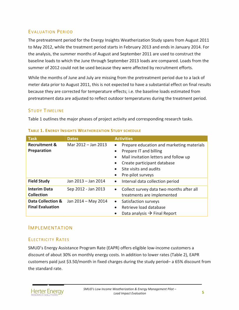
STUDY TIMELINE
Table 1 outlines the major phases of project activity and corresponding research tasks.
TABLE 1. ENERGY INSIGHTS WEATHERIZATION STUDY SCHEDULE
Task Dates Activities
Recruitment & Preparation
Mar 2012 – Jan 2013 Prepare education and marketing materials
Prepare IT and billing
Mail invitation letters and follow up
Create participant database
Site visits and audits
Pre‐pilot surveys
Field Study Jan 2013 – Jan 2014 Interval data collection period
Interim Data Collection
Sep 2012 ‐ Jan 2013 Collect survey data two months after all treatments are implemented
Data Collection & Final Evaluation
Jan 2014 – May 2014 Satisfaction surveys
Retrieve load database
Data analysis Final Report
IMPLEMENTATION
ELECTRICITY RATES
SMUD’s Energy Assistance Program Rate (EAPR) offers eligible low‐income customers a
discount of about 30% on monthly energy costs. In addition to lower rates (Table 2), EAPR
customers paid just $3.50/month in fixed charges during the study period– a 65% discount from
the standard rate.
SMUD’s Low Income Weatherization & Energy Management Pilot – Load Impact Evaluation
6
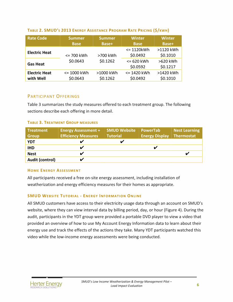
TABLE 2. SMUD’S 2013 ENERGY ASSISTANCE PROGRAM RATE PRICING ($/KWH)
Rate Code Summer Base
Summer Base+
Winter Base
Winter Base+
Electric Heat <= 700 kWh $0.0643
>700 kWh $0.1262
<= 1120kWh $0.0492
>1120 kWh $0.1010
Gas Heat <= 620 kWh $0.0592
>620 kWh $0.1217
Electric Heat with Well
<= 1000 kWh $0.0643
>1000 kWh $0.1262
<= 1420 kWh $0.0492
>1420 kWh $0.1010
PARTICIPANT OFFERINGS
Table 3 summarizes the study measures offered to each treatment group. The following
sections describe each offering in more detail.
TABLE 3. TREATMENT GROUP MEASURES
Treatment Group
Energy Assessment + Efficiency Measures
SMUD Website Tutorial
PowerTab Energy Display
Nest Learning Thermostat
YDT ✔ ✔
IHD ✔ ✔
Nest ✔ ✔
Audit (control) ✔
HOME ENERGY ASSESSMENT
All participants received a free on‐site energy assessment, including installation of
weatherization and energy efficiency measures for their homes as appropriate.
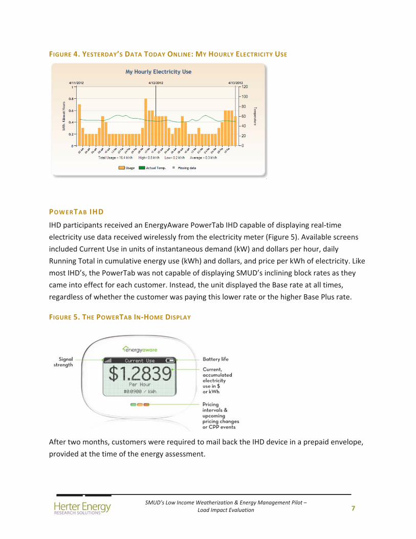
SMUD WEBSITE TUTORIAL ‐ ENERGY INFORMATION ONLINE
All SMUD customers have access to their electricity usage data through an account on SMUD’s
website, where they can view interval data by billing period, day, or hour (Figure 4). During the
audit, participants in the YDT group were provided a portable DVD player to view a video that
provided an overview of how to use My Account Energy Information data to learn about their
energy use and track the effects of the actions they take. Many YDT participants watched this
video while the low‐income energy assessments were being conducted.
SMUD’s Low Income Weatherization & Energy Management Pilot – Load Impact Evaluation
7
FIGURE 4. YESTERDAY’S DATA TODAY ONLINE: MY HOURLY ELECTRICITY USE
POWERTAB IHD
IHD participants received an EnergyAware PowerTab IHD capable of displaying real‐time
electricity use data received wirelessly from the electricity meter (Figure 5). Available screens
included Current Use in units of instantaneous demand (kW) and dollars per hour, daily
Running Total in cumulative energy use (kWh) and dollars, and price per kWh of electricity. Like
most IHD’s, the PowerTab was not capable of displaying SMUD’s inclining block rates as they
came into effect for each customer. Instead, the unit displayed the Base rate at all times,
regardless of whether the customer was paying this lower rate or the higher Base Plus rate.
FIGURE 5. THE POWERTAB IN‐HOME DISPLAY
After two months, customers were required to mail back the IHD device in a prepaid envelope,
provided at the time of the energy assessment.
SMUD’s Low Income Weatherization & Energy Management Pilot – Load Impact Evaluation
8
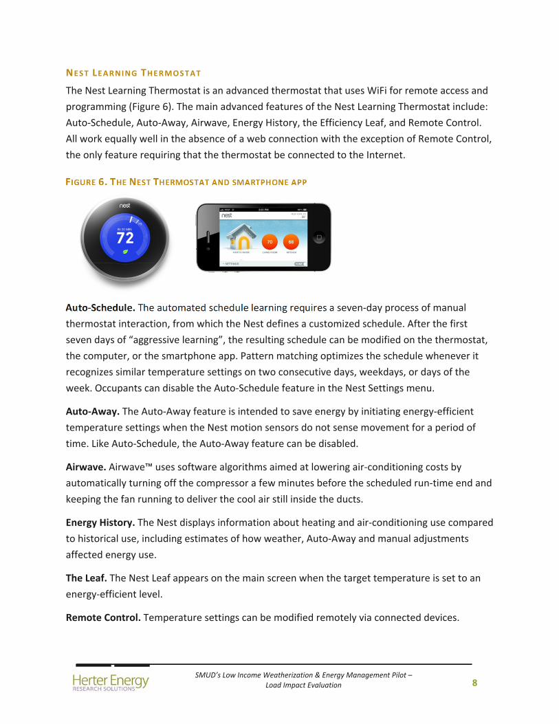
NEST LEARNING THERMOSTAT
The Nest Learning Thermostat is an advanced thermostat that uses WiFi for remote access and
programming (Figure 6). The main advanced features of the Nest Learning Thermostat include:
Auto‐Schedule, Auto‐Away, Airwave, Energy History, the Efficiency Leaf, and Remote Control.
All work equally well in the absence of a web connection with the exception of Remote Control,
the only feature requiring that the thermostat be connected to the Internet.
FIGURE 6. THE NEST THERMOSTAT AND SMARTPHONE APP
Auto‐Schedule. The automated schedule learning requires a seven‐day process of manual
thermostat interaction, from which the Nest defines a customized schedule. After the first
seven days of “aggressive learning”, the resulting schedule can be modified on the thermostat,
the computer, or the smartphone app. Pattern matching optimizes the schedule whenever it
recognizes similar temperature settings on two consecutive days, weekdays, or days of the
week. Occupants can disable the Auto‐Schedule feature in the Nest Settings menu.
Auto‐Away. The Auto‐Away feature is intended to save energy by initiating energy‐efficient
temperature settings when the Nest motion sensors do not sense movement for a period of
time. Like Auto‐Schedule, the Auto‐Away feature can be disabled.
Airwave. Airwave™ uses software algorithms aimed at lowering air‐conditioning costs by
automatically turning off the compressor a few minutes before the scheduled run‐time end and
keeping the fan running to deliver the cool air still inside the ducts.
Energy History. The Nest displays information about heating and air‐conditioning use compared
to historical use, including estimates of how weather, Auto‐Away and manual adjustments
affected energy use.
The Leaf. The Nest Leaf appears on the main screen when the target temperature is set to an
energy‐efficient level.
Remote Control. Temperature settings can be modified remotely via connected devices.

SMUD’s Low Income Weatherization & Energy Management Pilot – Load Impact Evaluation
9
THERMOSTAT INSTALLATION
An outside contractor with HVAC and networking installation experience was responsible for
scheduling appointments, installing thermostats, maintaining inventory, and servicing the
thermostats after installation. During installation, the customer filled out the Pre‐pilot Survey
and watched a video designed to educate participants on the smart thermostat technology. The
installer collected the completed surveys from the participants and returned them to SMUD.
MARKET RESEARCH
All pilot participants were required to fill out paper surveys while the energy advisor conducted
the energy assessment. This Pre‐Pilot Survey collected participant information in the following
categories:
Household demographics
Dwelling structural characteristics and appliances (collected by auditor)
Energy saving strategies
Energy knowledge
At the end of the study, participants were asked to complete the Post‐Pilot Survey, which
measured post‐treatment energy literacy, possible changes in energy‐related behavior,
perceived effort and savings, evaluation of technology, frequency of interaction, and attitudes
toward program and SMUD.
A summary and analysis of market research data can be found in Energy Insights
Weatherization Pilot Program Final Report (True North Research 2014).
SMUD’s Low Income Weatherization & Energy Management Pilot – Load Impact Evaluation
10
2. DATA
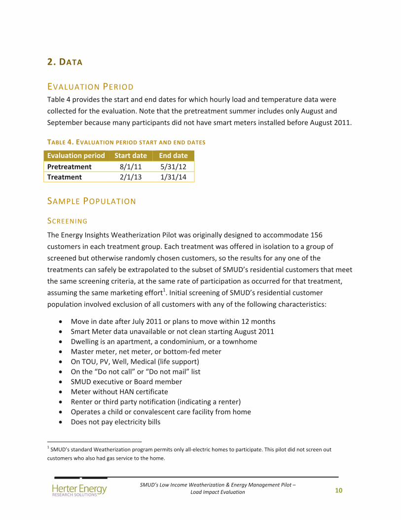
EVALUATION PERIOD Table 4 provides the start and end dates for which hourly load and temperature data were
collected for the evaluation. Note that the pretreatment summer includes only August and
September because many participants did not have smart meters installed before August 2011.
TABLE 4. EVALUATION PERIOD START AND END DATES
Evaluation period Start date End date
Pretreatment 8/1/11 5/31/12
Treatment 2/1/13 1/31/14
SAMPLE POPULATION
SCREENING
The Energy Insights Weatherization Pilot was originally designed to accommodate 156
customers in each treatment group. Each treatment was offered in isolation to a group of
screened but otherwise randomly chosen customers, so the results for any one of the
treatments can safely be extrapolated to the subset of SMUD’s residential customers that meet
the same screening criteria, at the same rate of participation as occurred for that treatment,
assuming the same marketing effort1. Initial screening of SMUD’s residential customer
population involved exclusion of all customers with any of the following characteristics:
Move in date after July 2011 or plans to move within 12 months
Smart Meter data unavailable or not clean starting August 2011
Dwelling is an apartment, a condominium, or a townhome
Master meter, net meter, or bottom‐fed meter
On TOU, PV, Well, Medical (life support)
On the “Do not call” or “Do not mail” list
SMUD executive or Board member
Meter without HAN certificate
Renter or third party notification (indicating a renter)
Operates a child or convalescent care facility from home
Does not pay electricity bills
1 SMUD’s standard Weatherization program permits only all‐electric homes to participate. This pilot did not screen out
customers who also had gas service to the home.
SMUD’s Low Income Weatherization & Energy Management Pilot – Load Impact Evaluation
11
No access to the Internet
Participant in the ACLM program, Smart Pricing Options, EV Innovators pilot, Summer Solutions study, solar, Smart Meter Acceptance Test Group, or smart meter opt‐out
The 10,000 customers in the screened database were randomly assigned to one of five groups
such that roughly 6,600 customers were assigned to the participant groups and about 3,300
customers were assigned to the control group sample. Of the 1,650 customers in each
participant group, 1,500 randomly chosen customers were invited to participate in one of the
four treatment groups.
The 2,250 customers that submitted an application for participation (37.5% of those invited)
were further screened to ensure that each: lived at the dwelling and paid the bill; did not have
an energy assessment conducted after 6/12/2012; lived in a single‐family or mobile home; did
not plan to move before 12/31/2013; did not operate a child or convalescent business from the
home; had central heating and air conditioning; had access to the Internet via home, work,
mobile, or library; had at most two thermostats; and were able to read and speak English (or
have a family member interpret). At the end of this secondary screening, about 160 customers
remained in each treatment group. By the end of the summer, the Nest treatment group had
dropped to about 120 participants, due mainly to incompatible air‐conditioning equipment,
while the YDT, IHD, and Audit groups each maintained about 150 participants each.
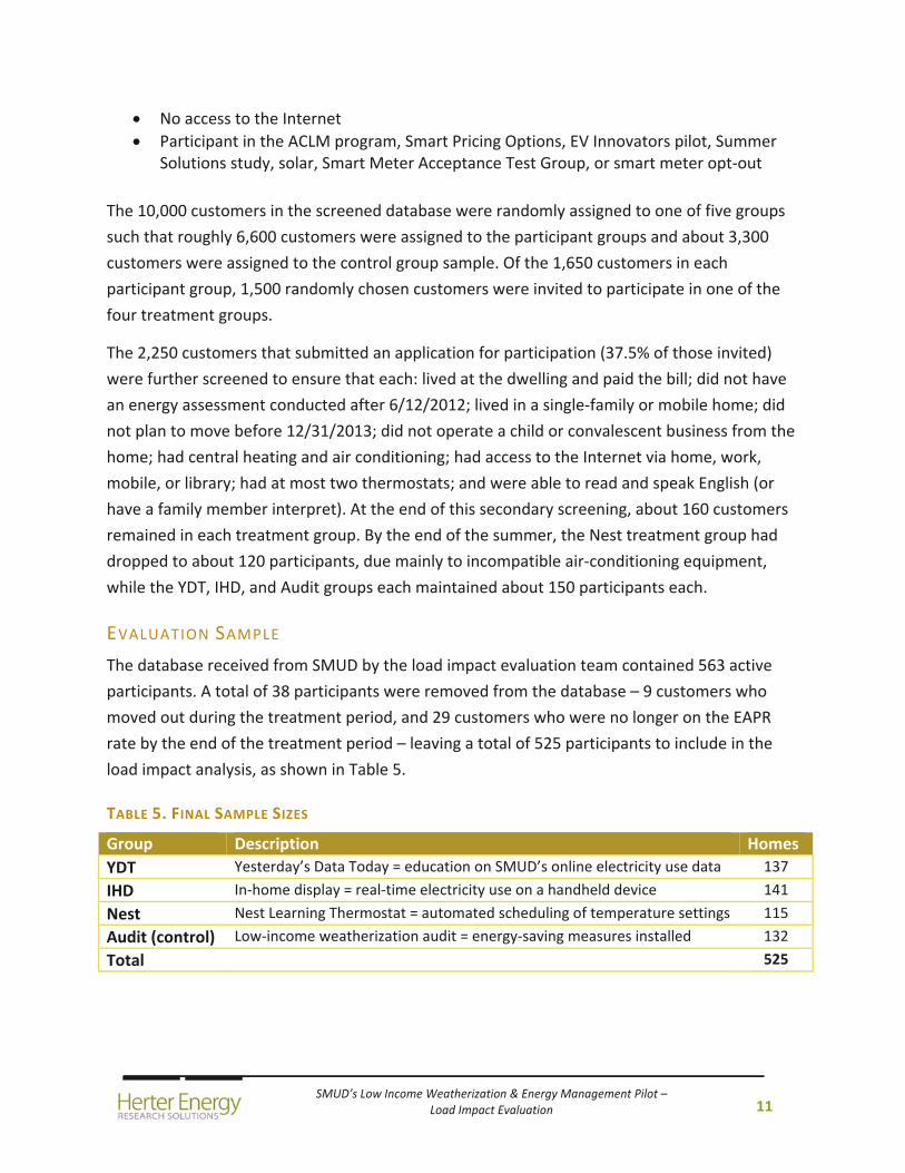
EVALUATION SAMPLE
The database received from SMUD by the load impact evaluation team contained 563 active
participants. A total of 38 participants were removed from the database – 9 customers who
moved out during the treatment period, and 29 customers who were no longer on the EAPR
rate by the end of the treatment period – leaving a total of 525 participants to include in the
load impact analysis, as shown in Table 5.
TABLE 5. FINAL SAMPLE SIZES
Group Description Homes
YDT Yesterday’s Data Today = education on SMUD’s online electricity use data 137
IHD In‐home display = real‐time electricity use on a handheld device 141
Nest Nest Learning Thermostat = automated scheduling of temperature settings 115
Audit (control) Low‐income weatherization audit = energy‐saving measures installed 132
Total 525
SMUD’s Low Income Weatherization & Energy Management Pilot – Load Impact Evaluation
12
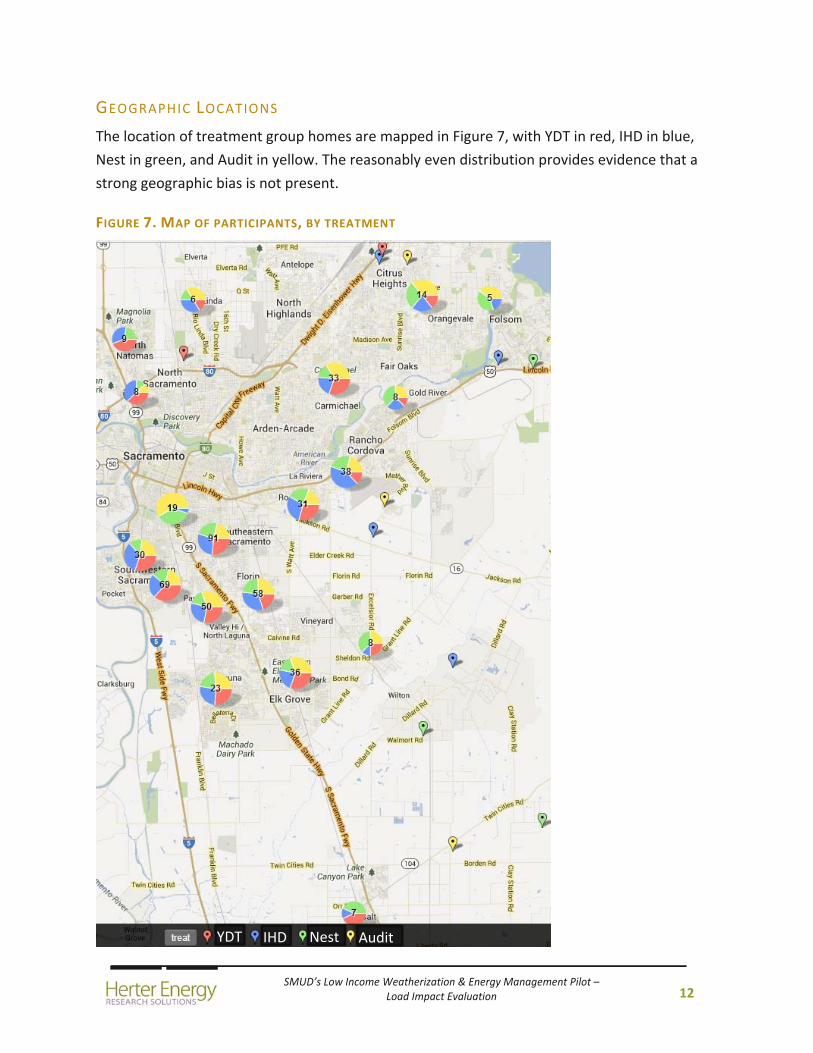
GEOGRAPHIC LOCATIONS
The location of treatment group homes are mapped in Figure 7, with YDT in red, IHD in blue,
Nest in green, and Audit in yellow. The reasonably even distribution provides evidence that a
strong geographic bias is not present.
FIGURE 7. MAP OF PARTICIPANTS, BY TREATMENT
YDT IHD Nest Audit
SMUD’s Low Income Weatherization & Energy Management Pilot – Load Impact Evaluation
13
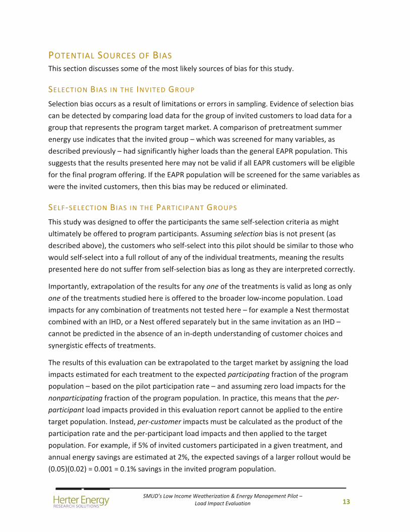
POTENTIAL SOURCES OF BIAS This section discusses some of the most likely sources of bias for this study.
SELECTION BIAS IN THE INVITED GROUP
Selection bias occurs as a result of limitations or errors in sampling. Evidence of selection bias
can be detected by comparing load data for the group of invited customers to load data for a
group that represents the program target market. A comparison of pretreatment summer
energy use indicates that the invited group – which was screened for many variables, as
described previously – had significantly higher loads than the general EAPR population. This
suggests that the results presented here may not be valid if all EAPR customers will be eligible
for the final program offering. If the EAPR population will be screened for the same variables as
were the invited customers, then this bias may be reduced or eliminated.
SELF‐SELECTION BIAS IN THE PARTICIPANT GROUPS
This study was designed to offer the participants the same self‐selection criteria as might
ultimately be offered to program participants. Assuming selection bias is not present (as
described above), the customers who self‐select into this pilot should be similar to those who
would self‐select into a full rollout of any of the individual treatments, meaning the results
presented here do not suffer from self‐selection bias as long as they are interpreted correctly.
Importantly, extrapolation of the results for any one of the treatments is valid as long as only
one of the treatments studied here is offered to the broader low‐income population. Load
impacts for any combination of treatments not tested here – for example a Nest thermostat
combined with an IHD, or a Nest offered separately but in the same invitation as an IHD –
cannot be predicted in the absence of an in‐depth understanding of customer choices and
synergistic effects of treatments.
The results of this evaluation can be extrapolated to the target market by assigning the load
impacts estimated for each treatment to the expected participating fraction of the program
population – based on the pilot participation rate – and assuming zero load impacts for the
nonparticipating fraction of the program population. In practice, this means that the per‐
participant load impacts provided in this evaluation report cannot be applied to the entire
target population. Instead, per‐customer impacts must be calculated as the product of the
participation rate and the per‐participant load impacts and then applied to the target
population. For example, if 5% of invited customers participated in a given treatment, and
annual energy savings are estimated at 2%, the expected savings of a larger rollout would be
(0.05)(0.02) = 0.001 = 0.1% savings in the invited program population.

SMUD’s Low Income Weatherization & Energy Management Pilot – Load Impact Evaluation
14
CONTROL GROUP BIAS
For experimental integrity and validity, a study should be designed from the outset as a random
control trial (RCT) or randomized encouragement design (RED). Where these are not possible,
other control group options must be considered. For this study, multiple control group options
are available. All have the potential to introduce bias in the results because the self‐selection
criteria (pilot offerings) differ between the participants and control group members.
CONTROL FOR TREATMENT EFFECTS
For this evaluation, the Audit group is used to correct for exogenous effects in the treatment
group loads. This group received all of the interventions experienced by the three treatment
groups with the exception of the treatments themselves; i.e. the Audit group did not receive
online training, an IHD, or a Nest thermostat. Use of the Audit group as the control has the
potential to introduce bias in the results because the self‐selection criteria (pilot offerings)
differ between the Audit and treatment group participants.
CONTROL FOR AUDIT EFFECTS
To assess the load impacts of the Audit group, a separate control group was needed. Three non‐
mutually‐exclusive groups were assessed, each drawn from the original randomly selected
control group sample described previously.
Geographically matched. A subset of customers was geographically selected to match
the participating customer locations by street. Since these customers were not invited
to participate and did not sign up for the study, variables of intention and willingness to
participate are likely to differ from those of the participants. In addition, central air‐
conditioning ownership is unknown for these customers, while participants were
required to have central air‐conditioning.
Surveyed. Another subset of the full control group completed a phone survey. These
survey respondents were screened for central air‐conditioning, which was one of the
survey questions. The potential for bias is further reduced due to the fact that there is
evidence of a willingness to participate by virtue of agreeing to answer the survey
questions by phone. Even so, there is uncertainty about whether the same types of
customers who answer a phone survey would sign up for the study, had they been
offered the opportunity to participate.
The potential impact of bias in the control group depends on its intended use. In the load
impact model used for this evaluation, the control group is used to correct for year‐over‐year
SMUD’s Low Income Weatherization & Energy Management Pilot – Load Impact Evaluation
15
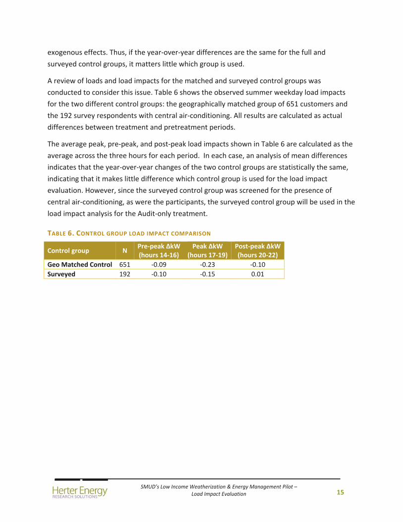
exogenous effects. Thus, if the year‐over‐year differences are the same for the full and
surveyed control groups, it matters little which group is used.
A review of loads and load impacts for the matched and surveyed control groups was
conducted to consider this issue. Table 6 shows the observed summer weekday load impacts
for the two different control groups: the geographically matched group of 651 customers and
the 192 survey respondents with central air‐conditioning. All results are calculated as actual
differences between treatment and pretreatment periods.
The average peak, pre‐peak, and post‐peak load impacts shown in Table 6 are calculated as the
average across the three hours for each period. In each case, an analysis of mean differences
indicates that the year‐over‐year changes of the two control groups are statistically the same,
indicating that it makes little difference which control group is used for the load impact
evaluation. However, since the surveyed control group was screened for the presence of
central air‐conditioning, as were the participants, the surveyed control group will be used in the
load impact analysis for the Audit‐only treatment.
TABLE 6. CONTROL GROUP LOAD IMPACT COMPARISON
Control group N Pre‐peak ΔkW(hours 14‐16)
Peak ΔkW (hours 17‐19)
Post‐peak ΔkW(hours 20‐22)
Geo Matched Control 651 ‐0.09 ‐0.23 ‐0.10
Surveyed 192 ‐0.10 ‐0.15 0.01
SMUD’s Low Income Weatherization & Energy Management Pilot – Load Impact Evaluation
16
LOAD DATA
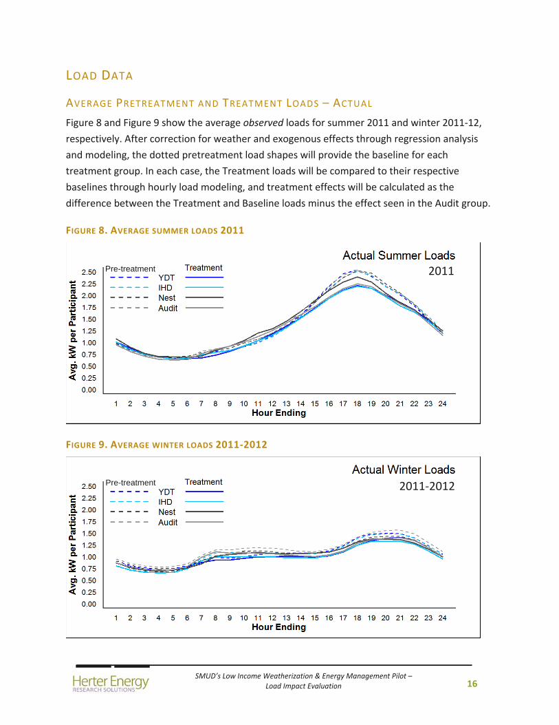
AVERAGE PRETREATMENT AND TREATMENT LOADS – ACTUAL
Figure 8 and Figure 9 show the average observed loads for summer 2011 and winter 2011‐12,
respectively. After correction for weather and exogenous effects through regression analysis
and modeling, the dotted pretreatment load shapes will provide the baseline for each
treatment group. In each case, the Treatment loads will be compared to their respective
baselines through hourly load modeling, and treatment effects will be calculated as the
difference between the Treatment and Baseline loads minus the effect seen in the Audit group.
FIGURE 8. AVERAGE SUMMER LOADS 2011
FIGURE 9. AVERAGE WINTER LOADS 2011‐2012
Pre-treatment
Pre-treatment
2011
2011‐2012
SMUD’s Low Income Weatherization & Energy Management Pilot – Load Impact Evaluation
17
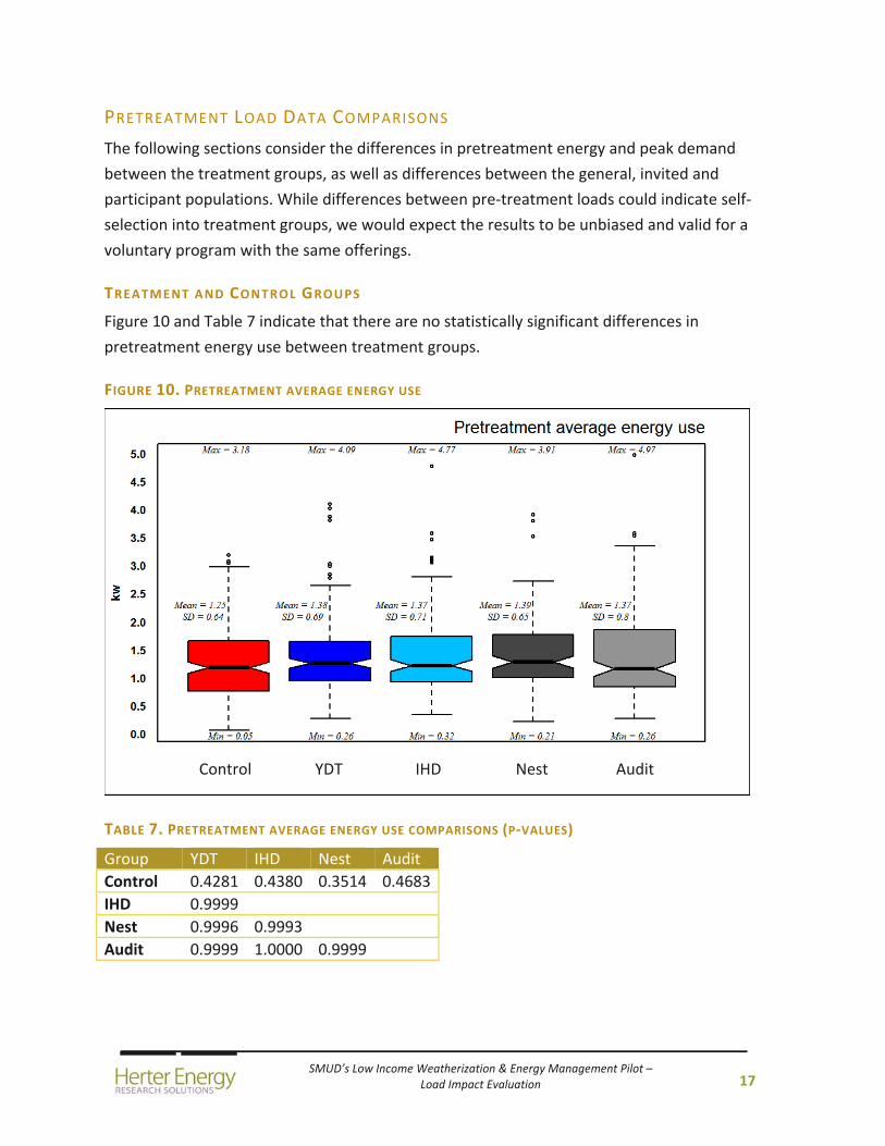
PRETREATMENT LOAD DATA COMPARISONS
The following sections consider the differences in pretreatment energy and peak demand
between the treatment groups, as well as differences between the general, invited and
participant populations. While differences between pre‐treatment loads could indicate self‐
selection into treatment groups, we would expect the results to be unbiased and valid for a
voluntary program with the same offerings.
TREATMENT AND CONTROL GROUPS
Figure 10 and Table 7 indicate that there are no statistically significant differences in
pretreatment energy use between treatment groups.
FIGURE 10. PRETREATMENT AVERAGE ENERGY USE
TABLE 7. PRETREATMENT AVERAGE ENERGY USE COMPARISONS (P‐VALUES)
Group YDT IHD Nest Audit
Control 0.4281 0.4380 0.3514 0.4683
IHD 0.9999
Nest 0.9996 0.9993
Audit 0.9999 1.0000 0.9999
Control YDT IHD Nest Audit
SMUD’s Low Income Weatherization & Energy Management Pilot – Load Impact Evaluation
18
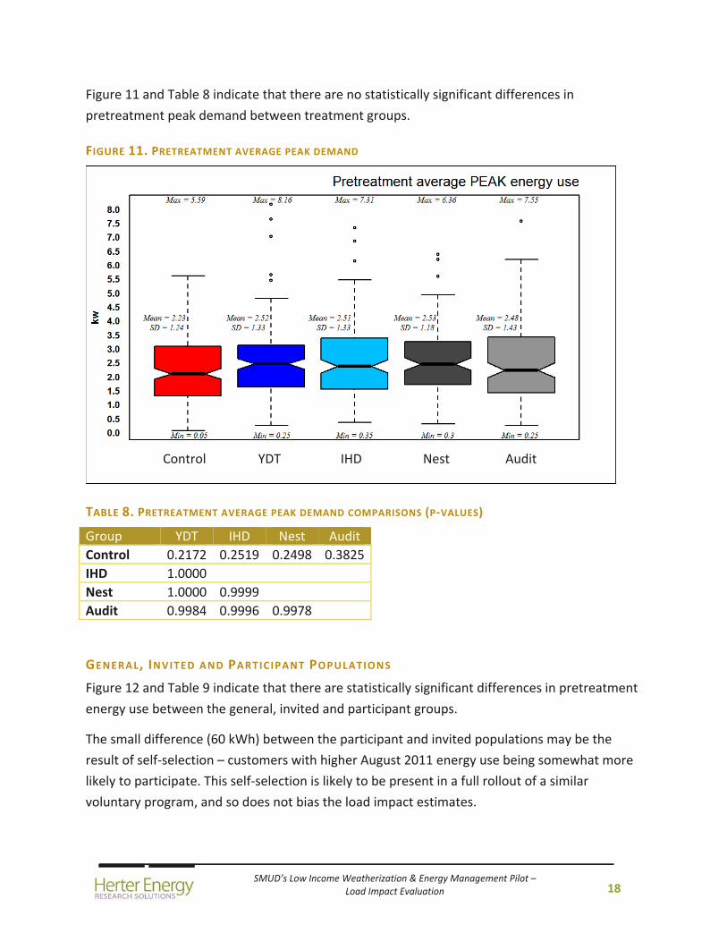
Figure 11 and Table 8 indicate that there are no statistically significant differences in
pretreatment peak demand between treatment groups.
FIGURE 11. PRETREATMENT AVERAGE PEAK DEMAND
TABLE 8. PRETREATMENT AVERAGE PEAK DEMAND COMPARISONS (P‐VALUES)
Group YDT IHD Nest Audit
Control 0.2172 0.2519 0.2498 0.3825
IHD 1.0000
Nest 1.0000 0.9999
Audit 0.9984 0.9996 0.9978
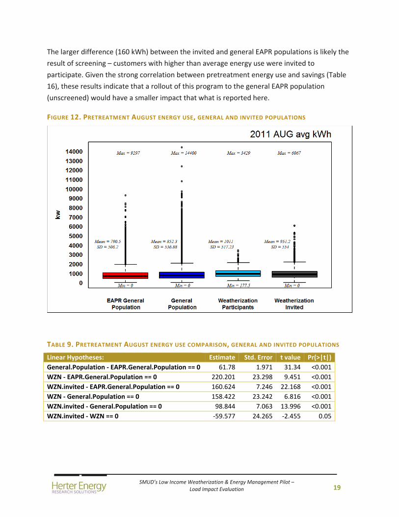
GENERAL, INVITED AND PARTICIPANT POPULATIONS
Figure 12 and Table 9 indicate that there are statistically significant differences in pretreatment
energy use between the general, invited and participant groups.
The small difference (60 kWh) between the participant and invited populations may be the
result of self‐selection – customers with higher August 2011 energy use being somewhat more
likely to participate. This self‐selection is likely to be present in a full rollout of a similar
voluntary program, and so does not bias the load impact estimates.
Control YDT IHD Nest Audit
SMUD’s Low Income Weatherization & Energy Management Pilot – Load Impact Evaluation
19
The larger difference (160 kWh) between the invited and general EAPR populations is likely the
result of screening – customers with higher than average energy use were invited to
participate. Given the strong correlation between pretreatment energy use and savings (Table
16), these results indicate that a rollout of this program to the general EAPR population
(unscreened) would have a smaller impact that what is reported here.
FIGURE 12. PRETREATMENT AUGUST ENERGY USE, GENERAL AND INVITED POPULATIONS
TABLE 9. PRETREATMENT AUGUST ENERGY USE COMPARISON, GENERAL AND INVITED POPULATIONS
Linear Hypotheses: Estimate Std. Error t value Pr(>|t|)
General.Population ‐ EAPR.General.Population == 0 61.78 1.971 31.34 <0.001
WZN ‐ EAPR.General.Population == 0 220.201 23.298 9.451 <0.001
WZN.invited ‐ EAPR.General.Population == 0 160.624 7.246 22.168 <0.001
WZN ‐ General.Population == 0 158.422 23.242 6.816 <0.001
WZN.invited ‐ General.Population == 0 98.844 7.063 13.996 <0.001
WZN.invited ‐ WZN == 0 ‐59.577 24.265 ‐2.455 0.05

SMUD’s Low Income Weatherization & Energy Management Pilot – Load Impact Evaluation
20
Figure 13 and Table 10 indicate that there is a statistically significant 0.384 kW difference in
pretreatment August peak demand between the invited and participant groups – likely the
result of self‐selection, such that customers with higher August 2011 peak demand were more
likely to participate. The same type of self‐selection is expected to be present in a full rollout of
a voluntary program, and so is not an indication of bias in the load impact estimates.
FIGURE 13. SUMMER PEAK DEMAND, INVITED POPULATION
TABLE 10. SUMMER PEAK DEMAND COMPARISON, PARTICIPANTS AND INVITED
Linear Hypotheses: Estimate Std. Error t value Pr(>|t|)
WZN.invited ‐ WZN == 0 ‐0.384 0.06186 ‐6.208 5.69E‐10
SMUD’s Low Income Weatherization & Energy Management Pilot – Load Impact Evaluation
21
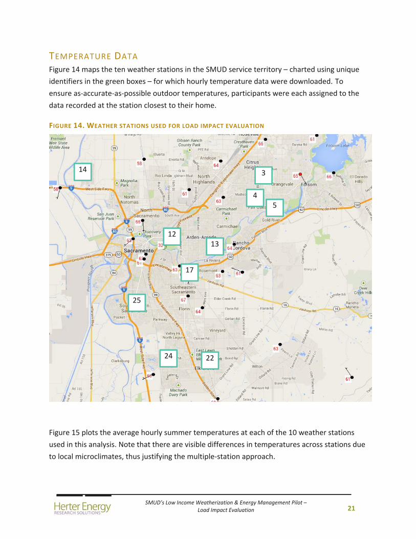
TEMPERATURE DATA Figure 14 maps the ten weather stations in the SMUD service territory – charted using unique
identifiers in the green boxes – for which hourly temperature data were downloaded. To
ensure as‐accurate‐as‐possible outdoor temperatures, participants were each assigned to the
data recorded at the station closest to their home.
FIGURE 14. WEATHER STATIONS USED FOR LOAD IMPACT EVALUATION
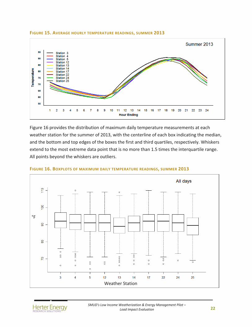
Figure 15 plots the average hourly summer temperatures at each of the 10 weather stations
used in this analysis. Note that there are visible differences in temperatures across stations due
to local microclimates, thus justifying the multiple‐station approach.
14 3
4 5
13
17
12
25
24 22
SMUD’s Low Income Weatherization & Energy Management Pilot – Load Impact Evaluation
22
FIGURE 15. AVERAGE HOURLY TEMPERATURE READINGS, SUMMER 2013
Figure 16 provides the distribution of maximum daily temperature measurements at each
weather station for the summer of 2013, with the centerline of each box indicating the median,
and the bottom and top edges of the boxes the first and third quartiles, respectively. Whiskers
extend to the most extreme data point that is no more than 1.5 times the interquartile range.
All points beyond the whiskers are outliers.
FIGURE 16. BOXPLOTS OF MAXIMUM DAILY TEMPERATURE READINGS, SUMMER 2013
Weather Station
°F
SMUD’s Low Income Weatherization & Energy Management Pilot – Load Impact Evaluation
23
3. ANALYSIS AND RESULTS
APPROACH
LOAD IMPACT ESTIMATION
Load impacts are estimated using the standard hourly load data collected by SMUD’s existing
metering infrastructure. The summer weekday, monthly, and seasonal load impact model
equations are given in Appendices B, C and D, respectively.
The model coefficients allow calculation of load values, while impact values are then calculated
as the difference‐in‐differences (DID) of the four load shapes as described in Equation 1. The
basic premise of DID evaluation is to compare the measure of interest at two points in time –
before and after treatment – in both the treatment and control groups, where the
pretreatment loads are normalized to treatment period temperatures.
EQUATION 1. CALCULATION OF LOAD IMPACTS
Load_Impactijk = (Part.treatijk – Part.pretreatijk) – (Control.treatijk – Control.pretreatijk)
Where, for customer i on day j at hour k: Load_Impactijk: estimate of hourly load change resulting from the treatment Part.treatijk: modeled average participant loads during the treatment period Part.pretreatijk: modeled average participant loads during the pretreatment period Control.treatijk: modeled average control loads during the treatment period Control.pretreatijk: modeled average control loads during the pretreatment period
This technique can be thought of as a within‐subjects estimate of the treatment effect
corrected for exogenous effects using the changes seen in the Audit control group, where both
are corrected for temperature differences between the pretreatment and treatment periods
using standard regression techniques. Without exogenous effects correction, a within‐subjects
comparison can overestimate or underestimate impacts by associating non‐treatment effects
with the treatment. For example, a downturn in the economy might cause an overall reduction
in residential electricity use. These exogenous energy savings must be removed from the
treatment group impacts using the control group impacts as a proxy for exogenous effects.
Otherwise, savings attributable to the treatment would be overestimated, when in fact much of
the savings was simply a result of the floundering economy.
An unbiased DID methodology requires that the composition of and exogenous inputs to the
treatment and control groups are as similar as possible. A standard method for accomplishing
this is a random control trial, whereby portions of the recruited population are randomly
SMUD’s Low Income Weatherization & Energy Management Pilot – Load Impact Evaluation
24
assigned to treatment and control groups. For the control group, treatment is then deferred to
a later date or denied altogether. Where a random control trial is not practical, as was the case
for this study, a control group can be selected to closely resemble the treatment group along a
subset of relevant variables. Such a control group, chosen or recruited under different
circumstances, is not without bias, however, because “willingness to participate” in the same
program as the participants is difficult or impossible to measure without putting the control
group through the same solicitation and recruitment process. In addition, Hawthorne effects
likely prevalent in the treatment group will not be seen in the control population.
The following sections provide the modeled loads and load impacts using this approach. For
consistency and ease of comparison, all loads and impacts are presented in units of average
kilowatt‐hours per hour (kWh/h), abbreviated in most cases to kW, where positive impact
values indicate an increase in energy use relative to the baseline, and negative impact values
indicate savings. Note that these hourly kW values are easily converted to kWh through
multiplication by the number of hours across the desired time period.
BILL IMPACT ESTIMATION
Bills are estimated for each customer by applying their individual electricity rate to their
modeled treatment and baseline loads as follows. Recall that 2011 summer loads are used as
the baseline because 2012 summer loads were affected by recruitment.
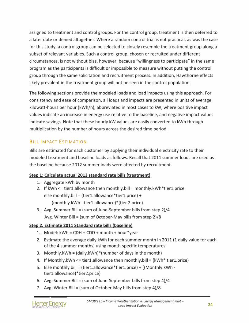
Step 1: Calculate actual 2013 standard rate bills (treatment)
1. Aggregate kWh by month 2. If kWh <= tier1.allowance then monthly.bill = monthly.kWh*tier1.price
else monthly.bill = (tier1.allowance*tier1.price) +
(monthly.kWh ‐ tier1.allowance)*(tier 2 price)
3. Avg. Summer Bill = (sum of June‐September bills from step 2)/4
Avg. Winter Bill = (sum of October‐May bills from step 2)/8
Step 2. Estimate 2011 Standard rate bills (baseline)
1. Model: kWh = CDH + CDD + month + hour*year
2. Estimate the average daily.kWh for each summer month in 2011 (1 daily value for each of the 4 summer months) using month‐specific temperatures
3. Monthly.kWh = (daily.kWh)*(number of days in the month)
4. If Monthly.kWh <= tier1.allowance then monthly.bill = (kWh* tier1.price)
5. Else monthly bill = (tier1.allowance*tier1.price) + ((Monthly.kWh ‐ tier1.allowance)*tier2.price)
6. Avg. Summer Bill = (sum of June‐September bills from step 4)/4
7. Avg. Winter Bill = (sum of October‐May bills from step 4)/8
SMUD’s Low Income Weatherization & Energy Management Pilot – Load Impact Evaluation
25
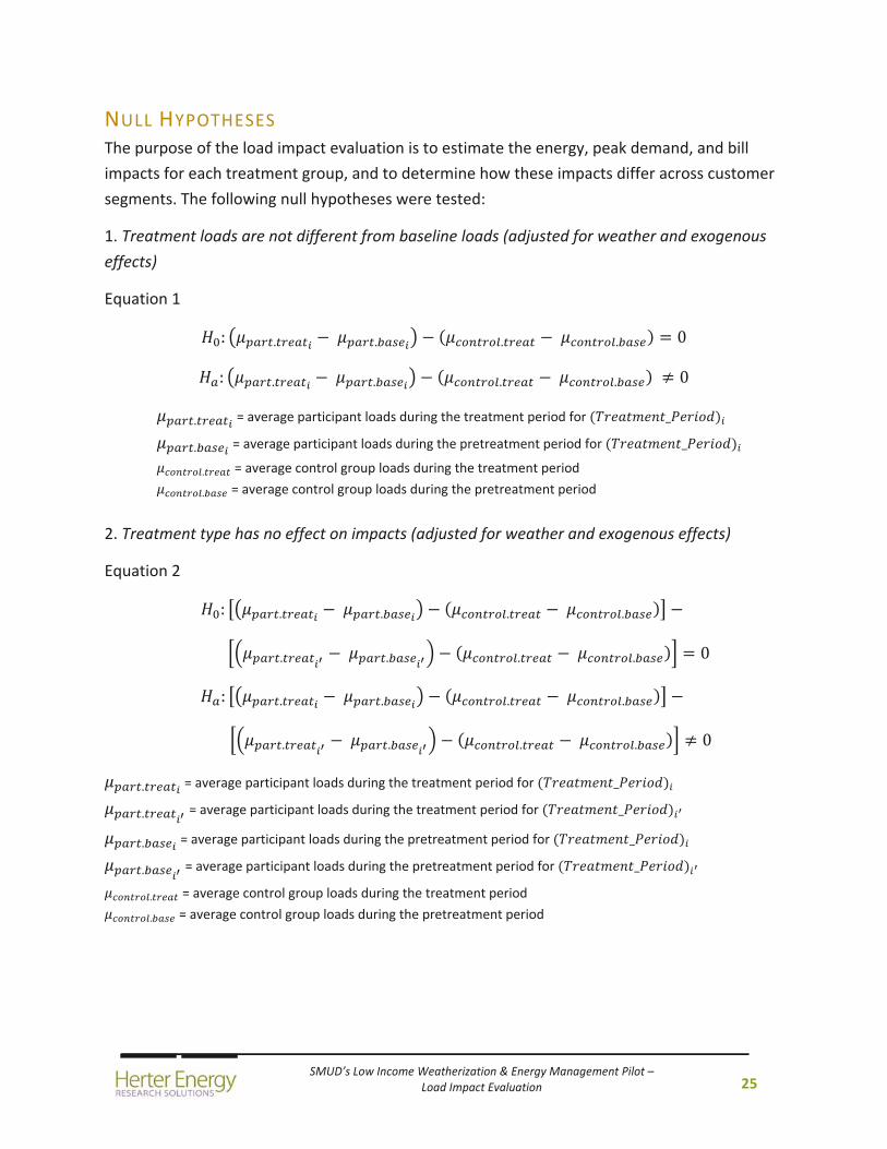
NULL HYPOTHESES The purpose of the load impact evaluation is to estimate the energy, peak demand, and bill
impacts for each treatment group, and to determine how these impacts differ across customer
segments. The following null hypotheses were tested:
1. Treatment loads are not different from baseline loads (adjusted for weather and exogenous
effects)
Equation 1
: . . . . 0
: . . . . 0
. = average participant loads during the treatment period for _
. = average participant loads during the pretreatment period for _
. = average control group loads during the treatment period
. = average control group loads during the pretreatment period
2. Treatment type has no effect on impacts (adjusted for weather and exogenous effects)
Equation 2
: . . . .
. . . . 0
: . . . .
. . . . 0
. = average participant loads during the treatment period for _
. = average participant loads during the treatment period for _
. = average participant loads during the pretreatment period for _
. = average participant loads during the pretreatment period for _
. = average control group loads during the treatment period
. = average control group loads during the pretreatment period
SMUD’s Low Income Weatherization & Energy Management Pilot – Load Impact Evaluation
26
LOAD IMPACTS OF THE AUDIT ONLY Although the main purpose of this evaluation is to determine the effects of the YDT, IHD, and
Nest treatments, SMUD is also interested in estimating the load impacts of the Audit group,
which received only the Low‐Income Weatherization Audit. Because gas‐heat customers have
been excluded from the pre‐existing weatherization program, results for gas and electric homes
are differentiated from each other.
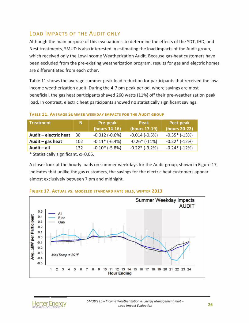
Table 11 shows the average summer peak load reduction for participants that received the low‐
income weatherization audit. During the 4‐7 pm peak period, where savings are most
beneficial, the gas heat participants shaved 260 watts (11%) off their pre‐weatherization peak
load. In contrast, electric heat participants showed no statistically significant savings.
TABLE 11. AVERAGE SUMMER WEEKDAY IMPACTS FOR THE AUDIT GROUP
Treatment N Pre‐peak (hours 14‐16)
Peak (hours 17‐19)
Post‐peak (hours 20‐22)
Audit – electric heat 30 ‐0.012 (‐0.6%) ‐0.014 (‐0.5%) ‐0.35* (‐13%)
Audit – gas heat 102 ‐0.11* (‐6.4%) ‐0.26* (‐11%) ‐0.22* (‐12%)
Audit – all 132 ‐0.10* (‐5.8%) ‐0.22* (‐9.2%) ‐0.24* (‐12%)
* Statistically significant, α=0.05.
A closer look at the hourly loads on summer weekdays for the Audit group, shown in Figure 17,
indicates that unlike the gas customers, the savings for the electric heat customers appear
almost exclusively between 7 pm and midnight.
FIGURE 17. ACTUAL VS. MODELED STANDARD RATE BILLS, WINTER 2013
SMUD’s Low Income Weatherization & Energy Management Pilot – Load Impact Evaluation
27
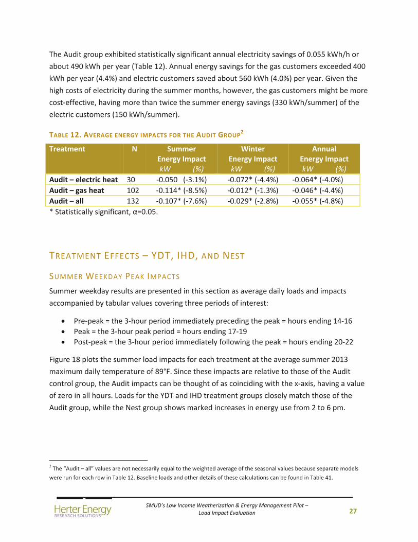
The Audit group exhibited statistically significant annual electricity savings of 0.055 kWh/h or
about 490 kWh per year (Table 12). Annual energy savings for the gas customers exceeded 400
kWh per year (4.4%) and electric customers saved about 560 kWh (4.0%) per year. Given the
high costs of electricity during the summer months, however, the gas customers might be more
cost‐effective, having more than twice the summer energy savings (330 kWh/summer) of the
electric customers (150 kWh/summer).
TABLE 12. AVERAGE ENERGY IMPACTS FOR THE AUDIT GROUP2
Treatment N Summer Energy Impact kW (%)
Winter Energy Impact kW (%)
Annual Energy Impact kW (%)
Audit – electric heat 30 ‐0.050 (‐3.1%) ‐0.072* (‐4.4%) ‐0.064* (‐4.0%)
Audit – gas heat 102 ‐0.114* (‐8.5%) ‐0.012* (‐1.3%) ‐0.046* (‐4.4%)
Audit – all 132 ‐0.107* (‐7.6%) ‐0.029* (‐2.8%) ‐0.055* (‐4.8%)
* Statistically significant, α=0.05.
TREATMENT EFFECTS – YDT, IHD, AND NEST
SUMMER WEEKDAY PEAK IMPACTS
Summer weekday results are presented in this section as average daily loads and impacts
accompanied by tabular values covering three periods of interest:
Pre‐peak = the 3‐hour period immediately preceding the peak = hours ending 14‐16
Peak = the 3‐hour peak period = hours ending 17‐19
Post‐peak = the 3‐hour period immediately following the peak = hours ending 20‐22
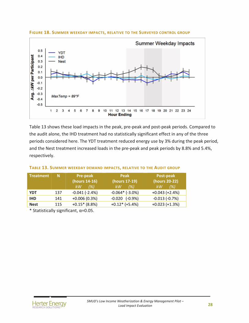
Figure 18 plots the summer load impacts for each treatment at the average summer 2013
maximum daily temperature of 89°F. Since these impacts are relative to those of the Audit
control group, the Audit impacts can be thought of as coinciding with the x‐axis, having a value
of zero in all hours. Loads for the YDT and IHD treatment groups closely match those of the
Audit group, while the Nest group shows marked increases in energy use from 2 to 6 pm.
2 The “Audit – all” values are not necessarily equal to the weighted average of the seasonal values because separate models
were run for each row in Table 12. Baseline loads and other details of these calculations can be found in Table 41.
SMUD’s Low Income Weatherization & Energy Management Pilot – Load Impact Evaluation
28
FIGURE 18. SUMMER WEEKDAY IMPACTS, RELATIVE TO THE SURVEYED CONTROL GROUP
Table 13 shows these load impacts in the peak, pre‐peak and post‐peak periods. Compared to
the audit alone, the IHD treatment had no statistically significant effect in any of the three
periods considered here. The YDT treatment reduced energy use by 3% during the peak period,
and the Nest treatment increased loads in the pre‐peak and peak periods by 8.8% and 5.4%,
respectively.
TABLE 13. SUMMER WEEKDAY DEMAND IMPACTS, RELATIVE TO THE AUDIT GROUP
Treatment N Pre‐peak (hours 14‐16) kW (%)
Peak (hours 17‐19) kW (%)
Post‐peak (hours 20‐22) kW (%)
YDT 137 ‐0.041 (‐2.4%) ‐0.064* (‐3.0%) +0.043 (+2.4%)
IHD 141 +0.006 (0.3%) ‐0.020 (‐0.9%) ‐0.013 (‐0.7%)
Nest 115 +0.15* (8.8%) +0.12* (+5.4%) +0.023 (+1.3%)
* Statistically significant, α=0.05.
SMUD’s Low Income Weatherization & Energy Management Pilot – Load Impact Evaluation
29
SEASONAL ENERGY AND BILL IMPACTS
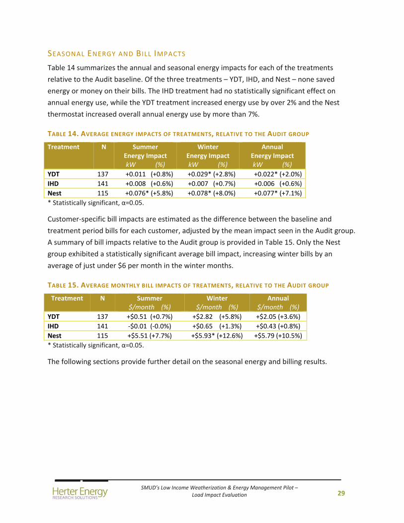
Table 14 summarizes the annual and seasonal energy impacts for each of the treatments
relative to the Audit baseline. Of the three treatments – YDT, IHD, and Nest – none saved
energy or money on their bills. The IHD treatment had no statistically significant effect on
annual energy use, while the YDT treatment increased energy use by over 2% and the Nest
thermostat increased overall annual energy use by more than 7%.
TABLE 14. AVERAGE ENERGY IMPACTS OF TREATMENTS, RELATIVE TO THE AUDIT GROUP
Treatment N Summer Energy Impact kW (%)
Winter Energy Impact kW (%)
Annual Energy Impact kW (%)
YDT 137 +0.011 (+0.8%) +0.029* (+2.8%) +0.022* (+2.0%)
IHD 141 +0.008 (+0.6%) +0.007 (+0.7%) +0.006 (+0.6%)
Nest 115 +0.076* (+5.8%) +0.078* (+8.0%) +0.077* (+7.1%)
* Statistically significant, α=0.05.
Customer‐specific bill impacts are estimated as the difference between the baseline and
treatment period bills for each customer, adjusted by the mean impact seen in the Audit group.
A summary of bill impacts relative to the Audit group is provided in Table 15. Only the Nest
group exhibited a statistically significant average bill impact, increasing winter bills by an
average of just under $6 per month in the winter months.
TABLE 15. AVERAGE MONTHLY BILL IMPACTS OF TREATMENTS, RELATIVE TO THE AUDIT GROUP
Treatment N Summer $/month (%)
Winter $/month (%)
Annual $/month (%)
YDT 137 +$0.51 (+0.7%) +$2.82 (+5.8%) +$2.05 (+3.6%)
IHD 141 ‐$0.01 (‐0.0%) +$0.65 (+1.3%) +$0.43 (+0.8%)
Nest 115 +$5.51 (+7.7%) +$5.93* (+12.6%) +$5.79 (+10.5%)
* Statistically significant, α=0.05.
The following sections provide further detail on the seasonal energy and billing results.

SMUD’s Low Income Weatherization & Energy Management Pilot – Load Impact Evaluation
30
SUMMER (JUNE – SEPTEMBER)
Figure 19 plots the hourly energy impacts for each treatment, calculated as the difference
between the hourly baseline and treatment load values. Summed across the 24 hours, only the
Nest group exhibited load impacts that were statistically different from the Audit group,
increasing summer energy use by 5.8% as shown in Table 14.
FIGURE 19. AVERAGE SUMMER ENERGY IMPACTS, RELATIVE TO THE AUDIT GROUP
Figure 20 shows that the distributions of summer bill impacts for the three treatment groups
are very similar.
FIGURE 20. BOXPLOT OF AVERAGE SUMMER BILL IMPACTS ($/MONTH)
SMUD’s Low Income Weatherization & Energy Management Pilot – Load Impact Evaluation
31
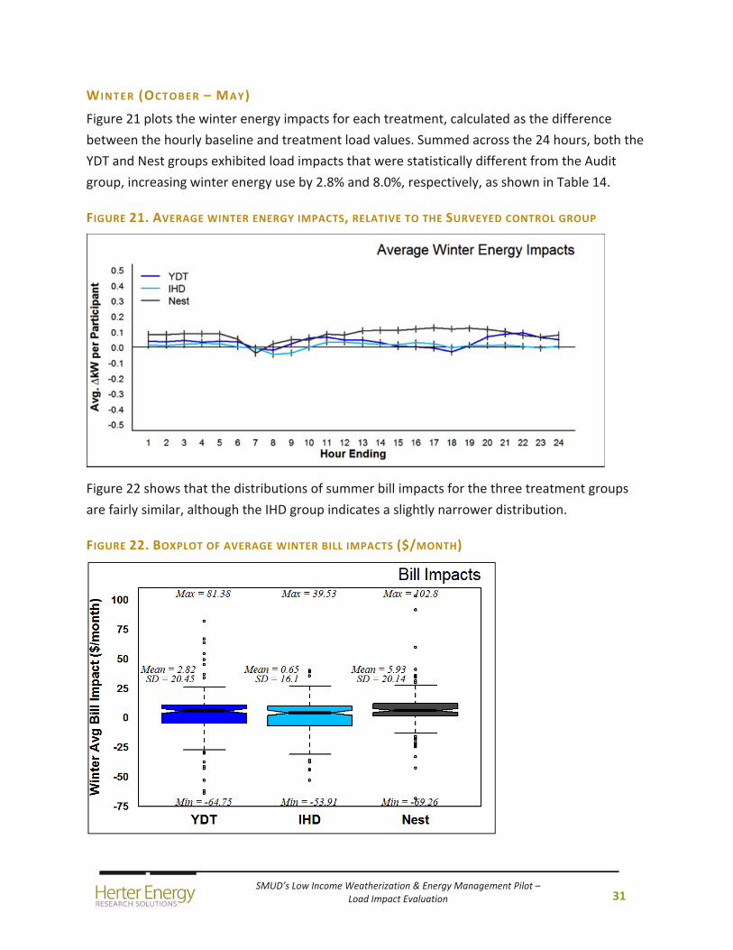
WINTER (OCTOBER – MAY)
Figure 21 plots the winter energy impacts for each treatment, calculated as the difference
between the hourly baseline and treatment load values. Summed across the 24 hours, both the
YDT and Nest groups exhibited load impacts that were statistically different from the Audit
group, increasing winter energy use by 2.8% and 8.0%, respectively, as shown in Table 14.
FIGURE 21. AVERAGE WINTER ENERGY IMPACTS, RELATIVE TO THE SURVEYED CONTROL GROUP
Figure 22 shows that the distributions of summer bill impacts for the three treatment groups
are fairly similar, although the IHD group indicates a slightly narrower distribution.
FIGURE 22. BOXPLOT OF AVERAGE WINTER BILL IMPACTS ($/MONTH)
SMUD’s Low Income Weatherization & Energy Management Pilot – Load Impact Evaluation
32
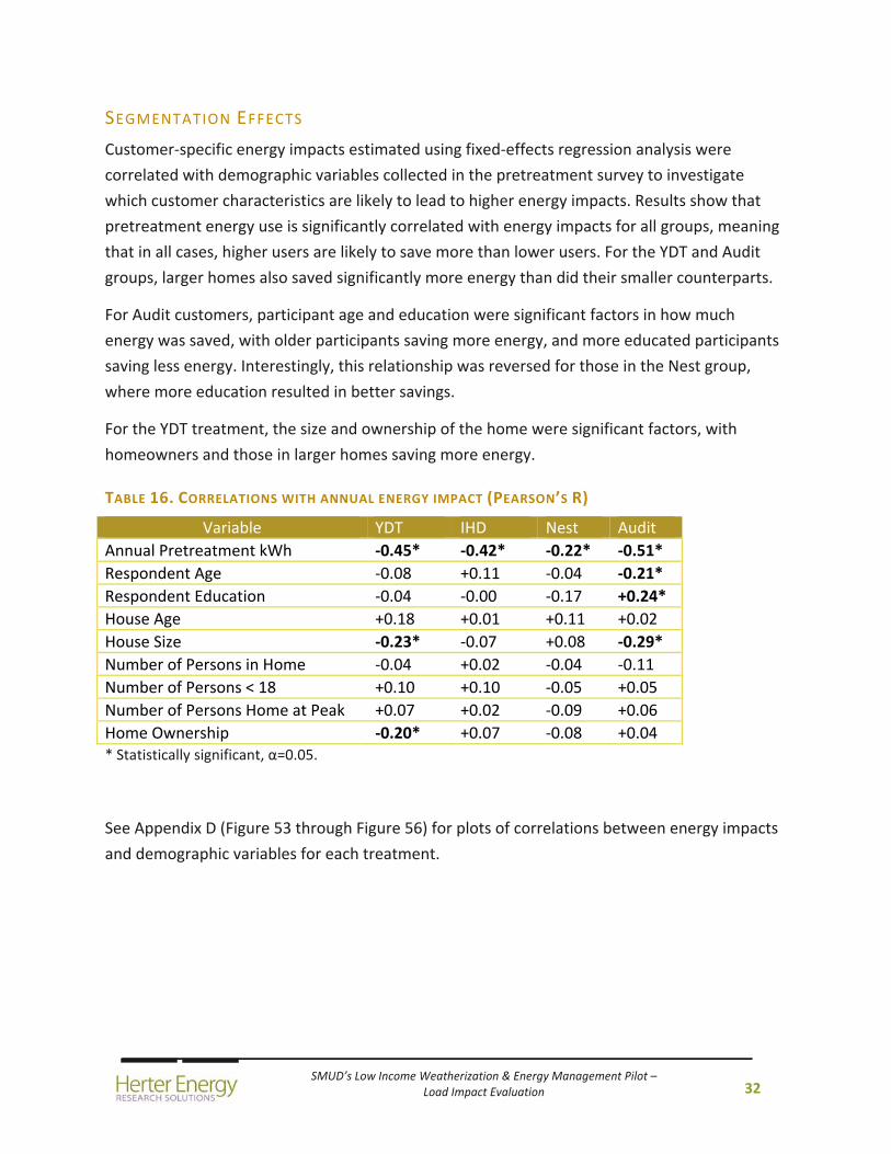
SEGMENTATION EFFECTS
Customer‐specific energy impacts estimated using fixed‐effects regression analysis were
correlated with demographic variables collected in the pretreatment survey to investigate
which customer characteristics are likely to lead to higher energy impacts. Results show that
pretreatment energy use is significantly correlated with energy impacts for all groups, meaning
that in all cases, higher users are likely to save more than lower users. For the YDT and Audit
groups, larger homes also saved significantly more energy than did their smaller counterparts.
For Audit customers, participant age and education were significant factors in how much
energy was saved, with older participants saving more energy, and more educated participants
saving less energy. Interestingly, this relationship was reversed for those in the Nest group,
where more education resulted in better savings.
For the YDT treatment, the size and ownership of the home were significant factors, with
homeowners and those in larger homes saving more energy.
TABLE 16. CORRELATIONS WITH ANNUAL ENERGY IMPACT (PEARSON’S R)
Variable YDT IHD Nest Audit
Annual Pretreatment kWh ‐0.45* ‐0.42* ‐0.22* ‐0.51*
Respondent Age ‐0.08 +0.11 ‐0.04 ‐0.21*
Respondent Education ‐0.04 ‐0.00 ‐0.17 +0.24*
House Age +0.18 +0.01 +0.11 +0.02
House Size ‐0.23* ‐0.07 +0.08 ‐0.29*
Number of Persons in Home ‐0.04 +0.02 ‐0.04 ‐0.11
Number of Persons < 18 +0.10 +0.10 ‐0.05 +0.05
Number of Persons Home at Peak +0.07 +0.02 ‐0.09 +0.06
Home Ownership ‐0.20* +0.07 ‐0.08 +0.04 * Statistically significant, α=0.05.
See Appendix D (Figure 53 through Figure 56) for plots of correlations between energy impacts
and demographic variables for each treatment.
SMUD’s Low Income Weatherization & Energy Management Pilot – Load Impact Evaluation
33
4. CONCLUSIONS This study investigated whether advanced smart grid devices and training would help low‐
income customers reduce their energy use and peak loads beyond what was saved under
SMUD’s standard Low‐Income Weatherization program. To this end, SMUD provided three
measures – smart thermostats (Nest), in‐home energy displays (IHD), and training in hourly
energy data use (YDT) – to about 400 homes on the low‐income Energy Assistance Program
Rate (EAPR). The three treatment groups – YDT, IHD, and Nest – received SMUD’s standard
Low‐Income Weatherization Audit in addition to the treatment of interest, while a fourth group
(Audit) received just the low‐income audit without smart grid devices or training.
During the summer peak hours of 4 to 7 p.m., participants in the Audit group saved a
statistically significant 220 watts on average, or 9.2% of their peak load. Relative to this value,
the YDT treatment saved an additional 64 watts (‐3.3%), the Nest treatment increased peak
loads by 120 watts (+5.4%), and the IHD treatment had no statistically significant effect.
Relative to the Audit alone, none of the three treatments saved energy. The YDT treatment
increased annual energy use by over 2%, and the Nest thermostat increased overall annual
energy use by more than 7%. Both of these increases are statistically significant. The IHD
treatment had no statistically significant effect on annual energy use.
Overall, the results of this study indicate that SMUD’s Low‐income Weatherization Audit
effectively reduced both summer and winter energy use for low‐income customers, resulting in
an annual energy savings of 4.8% and bill savings of about $50. Beyond the Audit, however,
training on SMUD’s Yesterday’s Data Today website (YDT), the provision of a real‐time energy
display (IHD), and the installation of a Nest Learning thermostat (Nest) were not effective in
reducing energy use, and in some cases showed evidence of increasing energy use.
The 7.1% annual energy increase for the low‐income customers provided with a Nest
thermostat are surprising given the 1.6% energy savings enjoyed by participants on the
standard rate who received Nest thermostats under SMUD’s Smart Thermostat pilot (Herter &
Okuneva 2014b).

SMUD’s Low Income Weatherization & Energy Management Pilot – Load Impact Evaluation
34
REFERENCES
Herter, K. and Y. Okuneva. 2014a. SMUD’s Communicating Thermostat Usability Study.
Prepared by Herter Energy Research Solutions for the Sacramento Municipal Utility District.
February.
Herter, K. and Y. Okuneva. 2014b. SMUD’s Smart Thermostat Pilot – Load Impact Evaluation.
Prepared by Herter Energy Research Solutions for the Sacramento Municipal Utility District.
August.
Smart Grid Consumer Collaborative. 2014. Spotlight on Low Income Consumers, Part II Summary
Report. April 10.
True North Research. 2014. Energy Insights Weatherization Pilot Program Final Report.
Prepared for the Sacramento Municipal Utility District. March 20.
SMUD’s Low Income Weatherization & Energy Management Pilot – Load Impact Evaluation
35
5. APPENDICES
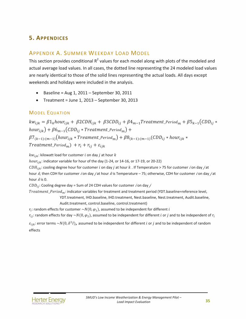
APPENDIX A. SUMMER WEEKDAY LOAD MODEL This section provides conditional R2 values for each model along with plots of the modeled and
actual average load values. In all cases, the dotted line representing the 24 modeled load values
are nearly identical to those of the solid lines representing the actual loads. All days except
weekends and holidays were included in the analysis.
Baseline = Aug 1, 2011 – September 30, 2011
Treatment = June 1, 2013 – September 30, 2013
MODEL EQUATION
1 2 3 4 _ 5 ∗
6 ∗ _
7 : ∗ _ 8 : ∗ ∗
_
: kilowatt load for customer on day at hour
: indicator variable for hour of the day (1‐24, or 14‐16, or 17‐19, or 20‐22)
: cooling degree hour for customer on day at hour . If Temperature > 75 for customer on day at
hour , then CDH for customer on day at hour is Temperature – 75; otherwise, CDH for customer on day at
hour is 0.
: Cooling degree day = Sum of 24 CDH values for customer on day
_ : indicator variables for treatment and treatment period (YDT.baseline=reference level,
YDT.treatment, IHD.baseline, IHD.treatment, Nest.baseline, Nest.treatment, Audit.baseline,
Audit.treatment, control.baseline, control.treatment)
: random effects for customer ~ 0, , assumed to be independent for different
: random effects for day ~ 0, , assumed to be independent for different or and to be independent of
: error terms ~ 0, , assumed to be independent for different or and to be independent of random
effects
SMUD’s Low Income Weatherization & Energy Management Pilot – Load Impact Evaluation
36
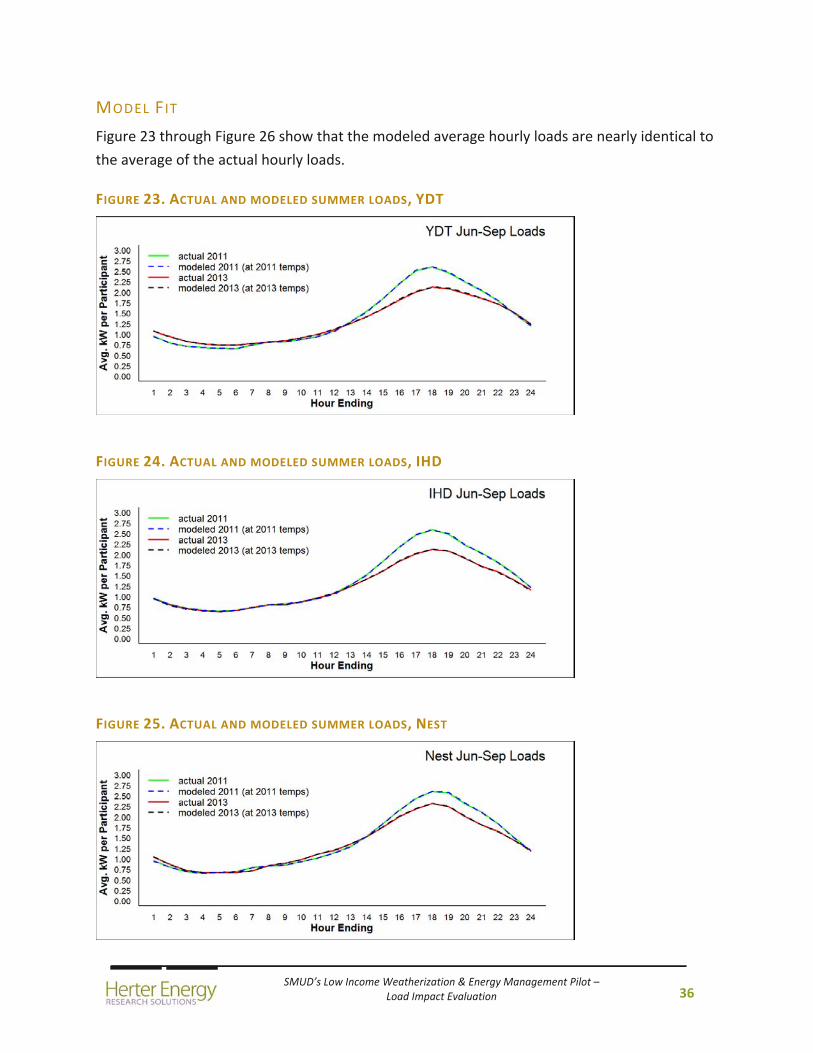
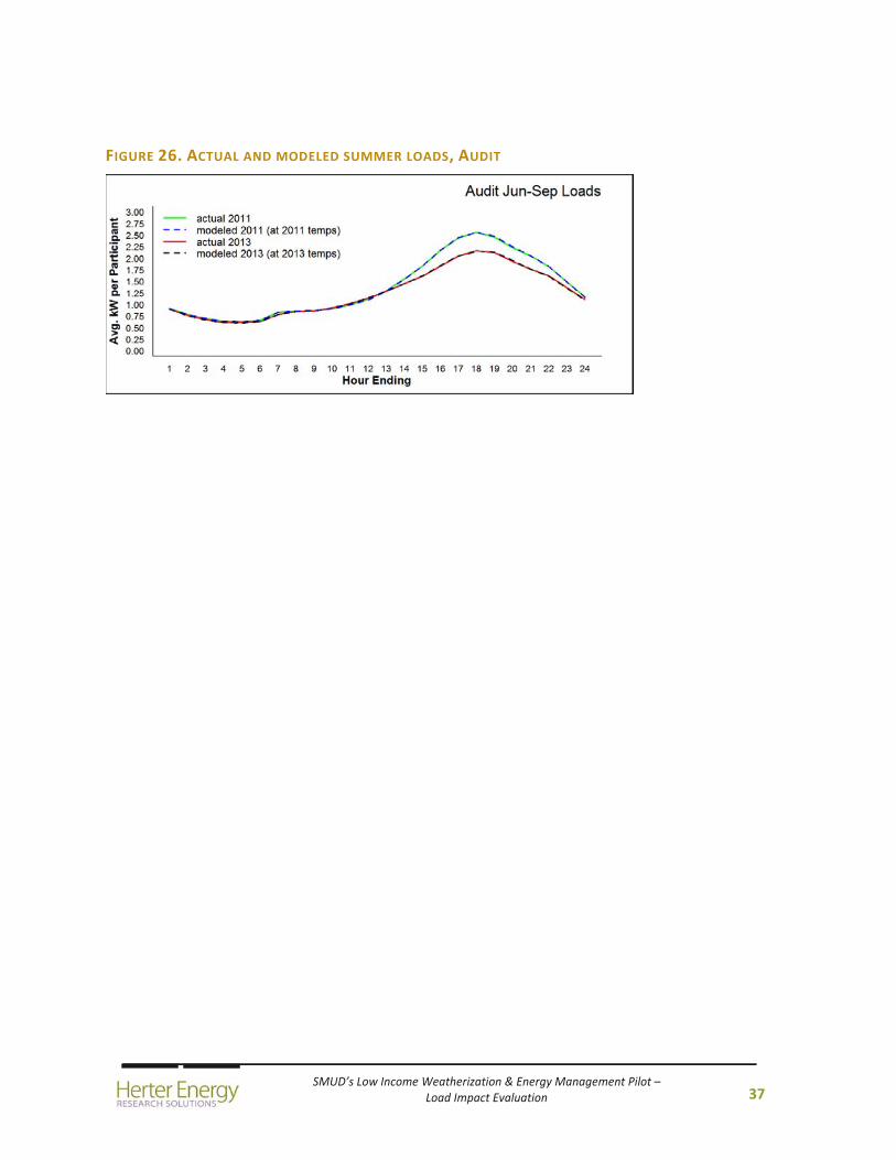
MODEL FIT
Figure 23 through Figure 26 show that the modeled average hourly loads are nearly identical to
the average of the actual hourly loads.
FIGURE 23. ACTUAL AND MODELED SUMMER LOADS, YDT
FIGURE 24. ACTUAL AND MODELED SUMMER LOADS, IHD
FIGURE 25. ACTUAL AND MODELED SUMMER LOADS, NEST
SMUD’s Low Income Weatherization & Energy Management Pilot – Load Impact Evaluation
37
FIGURE 26. ACTUAL AND MODELED SUMMER LOADS, AUDIT
SMUD’s Low Income Weatherization & Energy Management Pilot – Load Impact Evaluation
38
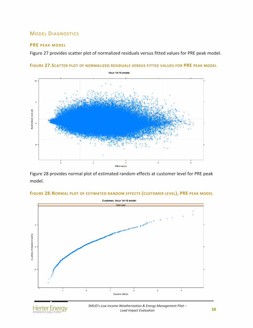
MODEL DIAGNOSTICS
PRE PEAK MODEL
Figure 27 provides scatter plot of normalized residuals versus fitted values for PRE peak model.
FIGURE 27.SCATTER PLOT OF NORMALIZED RESIDUALS VERSUS FITTED VALUES FOR PRE PEAK MODEL
Figure 28 provides normal plot of estimated random effects at customer level for PRE peak
model.
FIGURE 28.NORMAL PLOT OF ESTIMATED RANDOM EFFECTS (CUSTOMER LEVEL), PRE PEAK MODEL
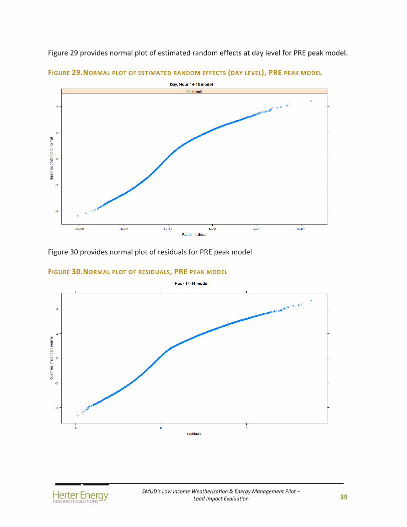
SMUD’s Low Income Weatherization & Energy Management Pilot – Load Impact Evaluation
39
Figure 29 provides normal plot of estimated random effects at day level for PRE peak model.
FIGURE 29.NORMAL PLOT OF ESTIMATED RANDOM EFFECTS (DAY LEVEL), PRE PEAK MODEL
Figure 30 provides normal plot of residuals for PRE peak model.
FIGURE 30.NORMAL PLOT OF RESIDUALS, PRE PEAK MODEL
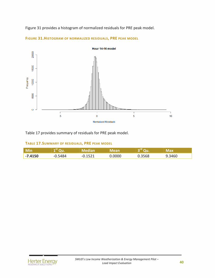
SMUD’s Low Income Weatherization & Energy Management Pilot – Load Impact Evaluation
40
Figure 31 provides a histogram of normalized residuals for PRE peak model.
FIGURE 31.HISTOGRAM OF NORMALIZED RESIDUALS, PRE PEAK MODEL
Table 17 provides summary of residuals for PRE peak model.
TABLE 17.SUMMARY OF RESIDUALS, PRE PEAK MODEL
Min 1st Qu. Median Mean 3rd Qu. Max
‐7.4150 ‐0.5484 ‐0.1521 0.0000 0.3568 9.3460
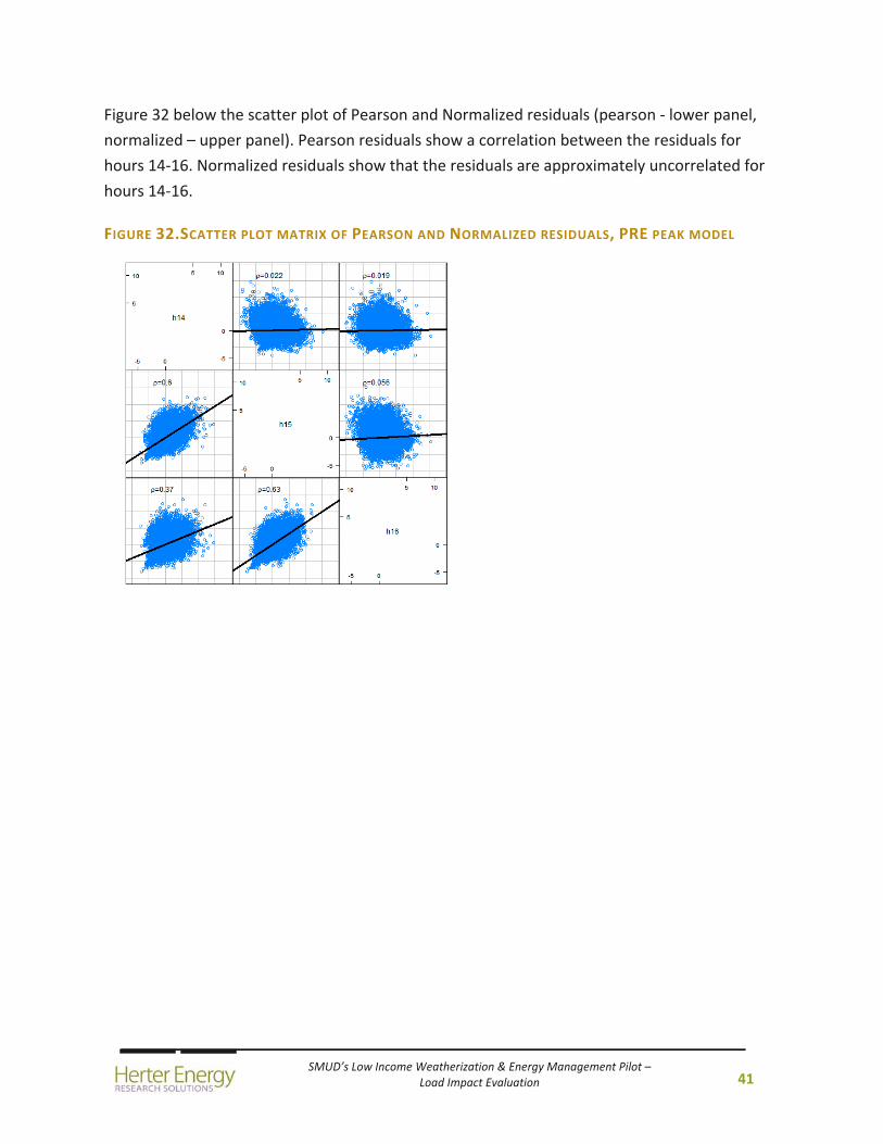
SMUD’s Low Income Weatherization & Energy Management Pilot – Load Impact Evaluation
41
Figure 32 below the scatter plot of Pearson and Normalized residuals (pearson ‐ lower panel,
normalized – upper panel). Pearson residuals show a correlation between the residuals for
hours 14‐16. Normalized residuals show that the residuals are approximately uncorrelated for
hours 14‐16.
FIGURE 32.SCATTER PLOT MATRIX OF PEARSON AND NORMALIZED RESIDUALS, PRE PEAK MODEL
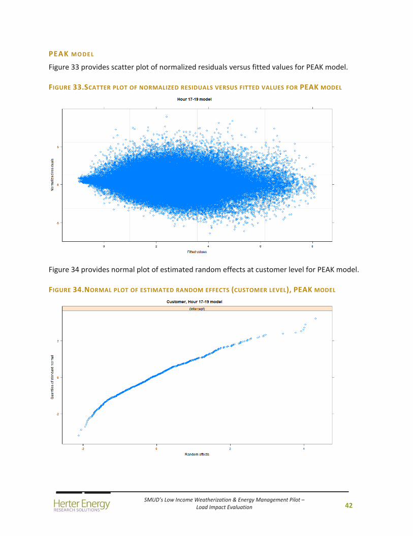
SMUD’s Low Income Weatherization & Energy Management Pilot – Load Impact Evaluation
42
PEAK MODEL
Figure 33 provides scatter plot of normalized residuals versus fitted values for PEAK model.
FIGURE 33.SCATTER PLOT OF NORMALIZED RESIDUALS VERSUS FITTED VALUES FOR PEAK MODEL
Figure 34 provides normal plot of estimated random effects at customer level for PEAK model.
FIGURE 34.NORMAL PLOT OF ESTIMATED RANDOM EFFECTS (CUSTOMER LEVEL), PEAK MODEL
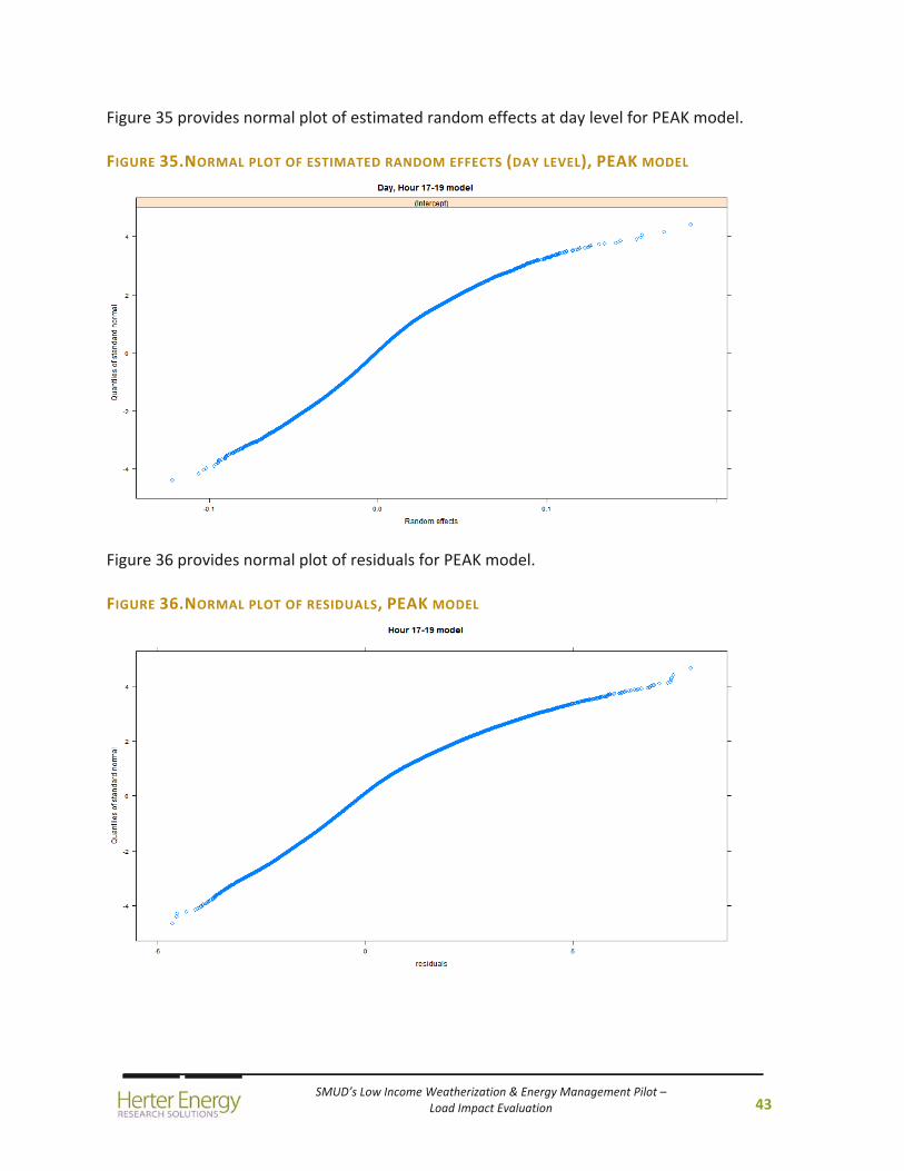
SMUD’s Low Income Weatherization & Energy Management Pilot – Load Impact Evaluation
43
Figure 35 provides normal plot of estimated random effects at day level for PEAK model.
FIGURE 35.NORMAL PLOT OF ESTIMATED RANDOM EFFECTS (DAY LEVEL), PEAK MODEL
Figure 36 provides normal plot of residuals for PEAK model.
FIGURE 36.NORMAL PLOT OF RESIDUALS, PEAK MODEL
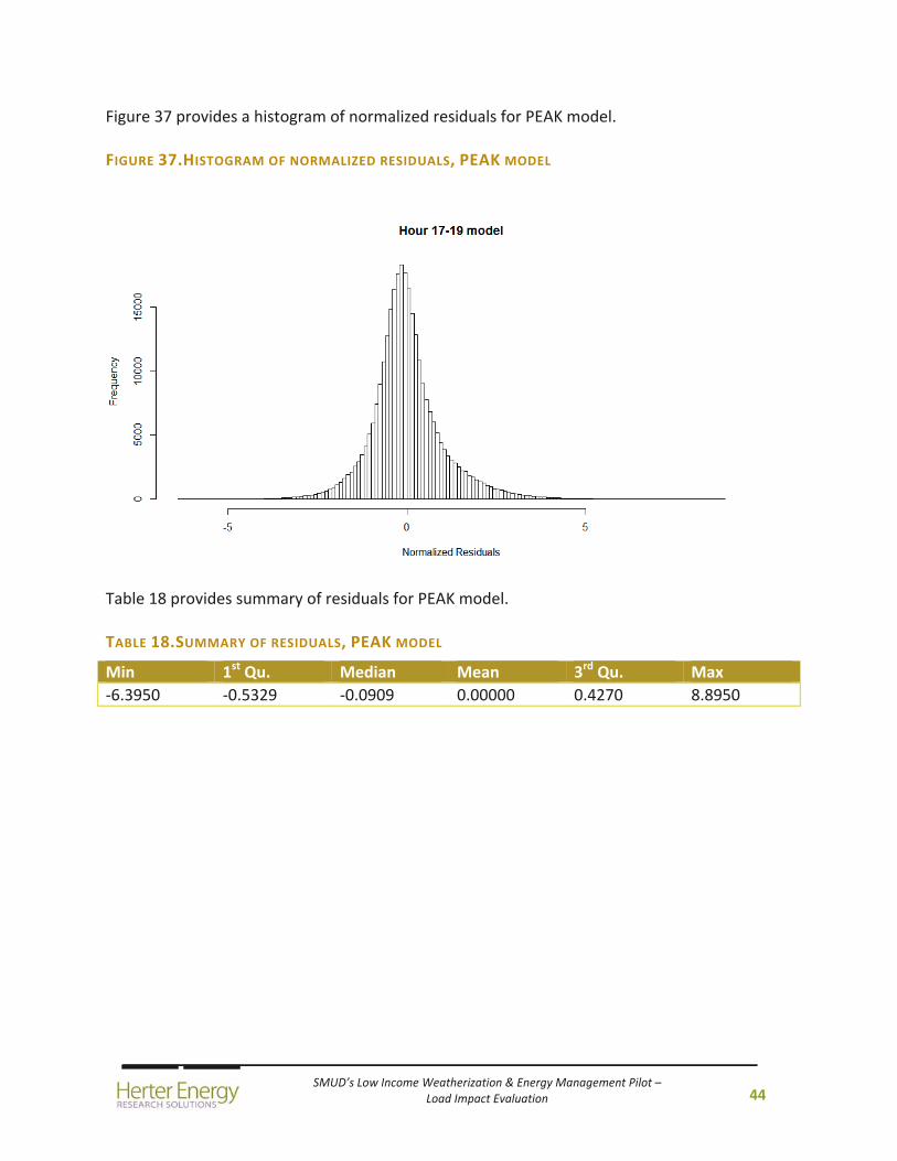
SMUD’s Low Income Weatherization & Energy Management Pilot – Load Impact Evaluation
44
Figure 37 provides a histogram of normalized residuals for PEAK model.
FIGURE 37.HISTOGRAM OF NORMALIZED RESIDUALS, PEAK MODEL
Table 18 provides summary of residuals for PEAK model.
TABLE 18.SUMMARY OF RESIDUALS, PEAK MODEL
Min 1st Qu. Median Mean 3rd Qu. Max
‐6.3950 ‐0.5329 ‐0.0909 0.00000 0.4270 8.8950
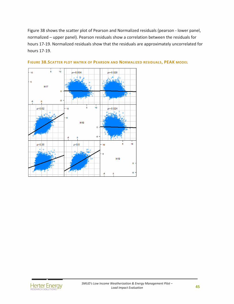
SMUD’s Low Income Weatherization & Energy Management Pilot – Load Impact Evaluation
45
Figure 38 shows the scatter plot of Pearson and Normalized residuals (pearson ‐ lower panel,
normalized – upper panel). Pearson residuals show a correlation between the residuals for
hours 17‐19. Normalized residuals show that the residuals are approximately uncorrelated for
hours 17‐19.
FIGURE 38.SCATTER PLOT MATRIX OF PEARSON AND NORMALIZED RESIDUALS, PEAK MODEL
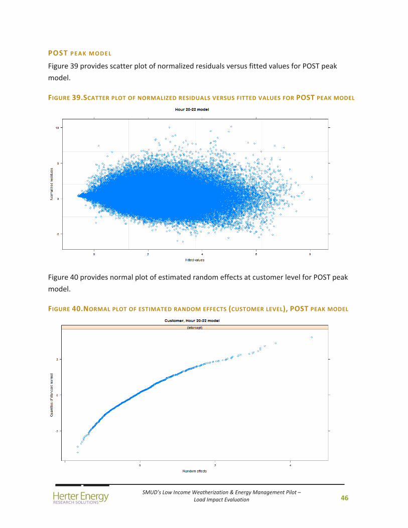
SMUD’s Low Income Weatherization & Energy Management Pilot – Load Impact Evaluation
46
POST PEAK MODEL
Figure 39 provides scatter plot of normalized residuals versus fitted values for POST peak
model.
FIGURE 39.SCATTER PLOT OF NORMALIZED RESIDUALS VERSUS FITTED VALUES FOR POST PEAK MODEL
Figure 40 provides normal plot of estimated random effects at customer level for POST peak
model.
FIGURE 40.NORMAL PLOT OF ESTIMATED RANDOM EFFECTS (CUSTOMER LEVEL), POST PEAK MODEL
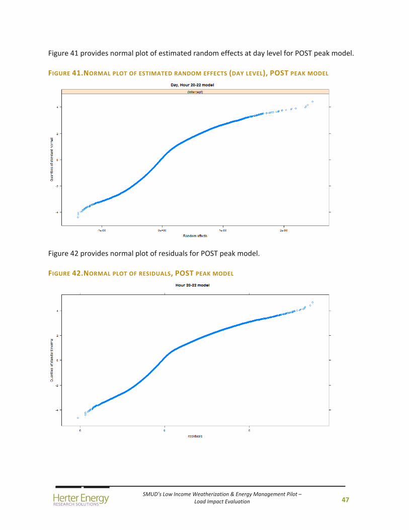
SMUD’s Low Income Weatherization & Energy Management Pilot – Load Impact Evaluation
47
Figure 41 provides normal plot of estimated random effects at day level for POST peak model.
FIGURE 41.NORMAL PLOT OF ESTIMATED RANDOM EFFECTS (DAY LEVEL), POST PEAK MODEL
Figure 42 provides normal plot of residuals for POST peak model.
FIGURE 42.NORMAL PLOT OF RESIDUALS, POST PEAK MODEL
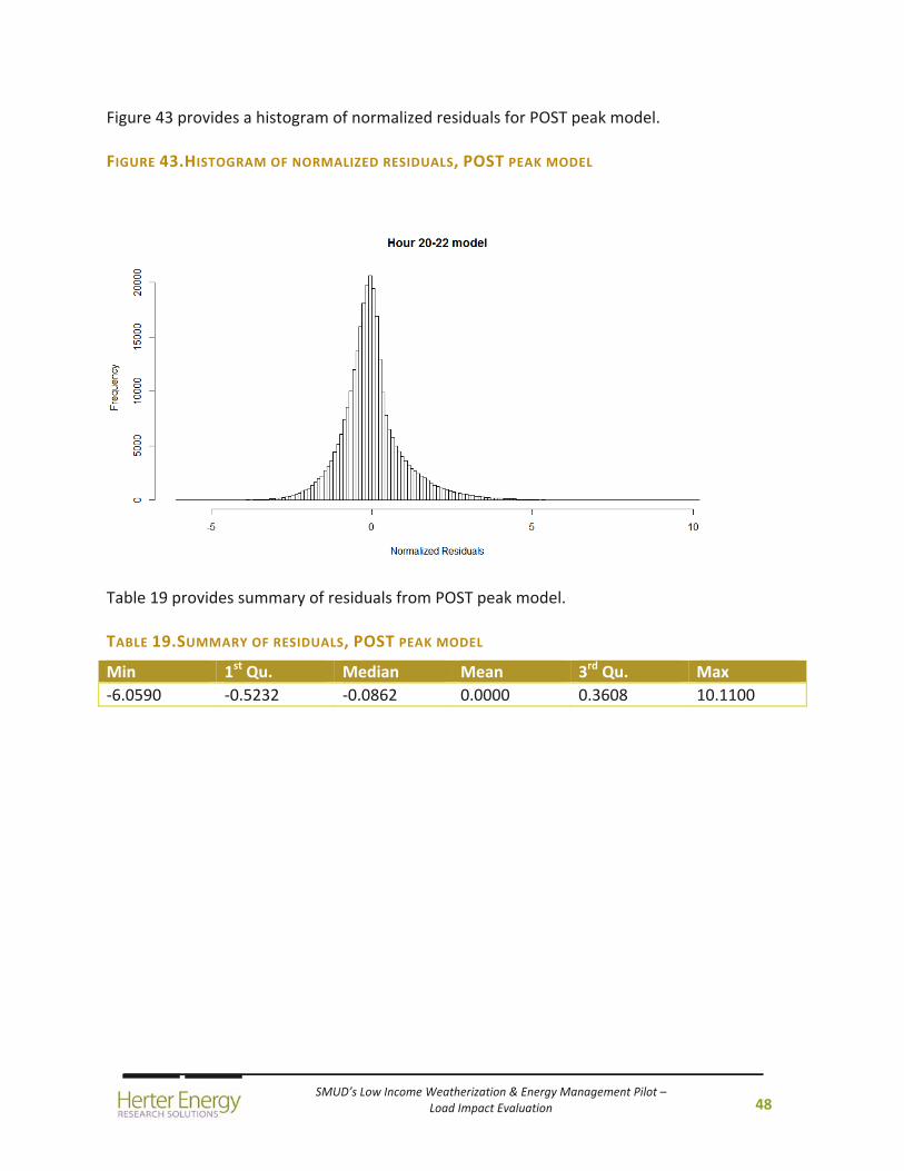
SMUD’s Low Income Weatherization & Energy Management Pilot – Load Impact Evaluation
48
Figure 43 provides a histogram of normalized residuals for POST peak model.
FIGURE 43.HISTOGRAM OF NORMALIZED RESIDUALS, POST PEAK MODEL
Table 19 provides summary of residuals from POST peak model.
TABLE 19.SUMMARY OF RESIDUALS, POST PEAK MODEL
Min 1st Qu. Median Mean 3rd Qu. Max
‐6.0590 ‐0.5232 ‐0.0862 0.0000 0.3608 10.1100
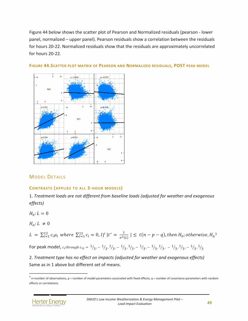
SMUD’s Low Income Weatherization & Energy Management Pilot – Load Impact Evaluation
49
Figure 44 below shows the scatter plot of Pearson and Normalized residuals (pearson ‐ lower
panel, normalized – upper panel). Pearson residuals show a correlation between the residuals
for hours 20‐22. Normalized residuals show that the residuals are approximately uncorrelated
for hours 20‐22.
FIGURE 44.SCATTER PLOT MATRIX OF PEARSON AND NORMALIZED RESIDUALS, POST PEAK MODEL
MODEL DETAILS
CONTRASTS (APPLIES TO ALL 3‐HOUR MODELS)
1. Treatment loads are not different from baseline loads (adjusted for weather and exogenous
effects)
: 0
: 0
∑ ∑ 0, | ∗ | , ; , 3
For peak model, 1 3 , 1 3 ,13 , 1 3 ,
13 , 1 3 , 1 3 ,
13 , 1 3 ,
13 , 1 3 ,
13
2. Treatment type has no effect on impacts (adjusted for weather and exogenous effects)
Same as in 1 above but different set of means.
3 n=number of observations, p = number of model parameters associated with fixed effects, q = number of covariance parameters with random
effects or correlations

SMUD’s Low Income Weatherization & Energy Management Pilot – Load Impact Evaluation
50
CONTRASTS EXAMPLES
YDT peak impact relative to baseline (adjusted for weather and exogenous effects), and
comparing YDT and IHD treatments peak impacts (adjusted for weather and pretreatment
differences)
1. Treatment loads are not different from baseline loads (adjusted for weather and exogenous
effects)
. . . . . . . . . . . . . . . . . .
3 . . . . . . . . . . . .
3
2. Treatment type has no effect on impacts (adjusted for weather and exogenous effects)
. . . . . . . . . . . . . . . . . .
3 . . . . . . . . . . . . . . . . . .
3
Notes:
′ are estimated using regression coefficients (provided below) with the temperature profile
of interest – average temp weekday summer 2013 days.
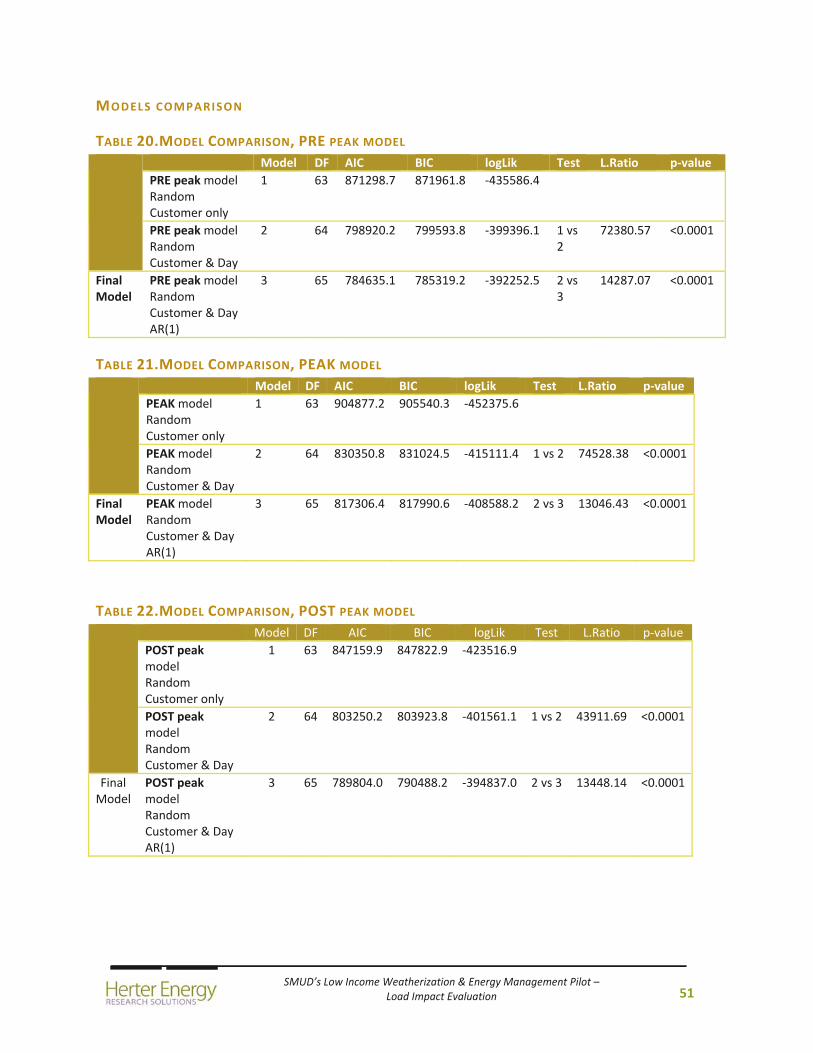
SMUD’s Low Income Weatherization & Energy Management Pilot – Load Impact Evaluation
51
MODELS COMPARISON
TABLE 20.MODEL COMPARISON, PRE PEAK MODEL
Model DF AIC BIC logLik Test L.Ratio p‐value
PRE peak model Random Customer only
1 63 871298.7 871961.8 ‐435586.4
PRE peak model Random Customer & Day
2 64 798920.2 799593.8 ‐399396.1 1 vs 2
72380.57 <0.0001
Final Model
PRE peak model Random Customer & Day AR(1)
3 65 784635.1 785319.2 ‐392252.5 2 vs 3
14287.07 <0.0001
TABLE 21.MODEL COMPARISON, PEAK MODEL
Model DF AIC BIC logLik Test L.Ratio p‐value
PEAK model Random Customer only
1 63 904877.2 905540.3 ‐452375.6
PEAK model Random Customer & Day
2 64 830350.8 831024.5 ‐415111.4 1 vs 2 74528.38 <0.0001
Final Model
PEAK model Random Customer & Day AR(1)
3 65 817306.4 817990.6 ‐408588.2 2 vs 3 13046.43 <0.0001
TABLE 22.MODEL COMPARISON, POST PEAK MODEL
Model DF AIC BIC logLik Test L.Ratio p‐value
POST peak model Random Customer only
1 63 847159.9 847822.9 ‐423516.9
POST peak model Random Customer & Day
2 64 803250.2 803923.8 ‐401561.1 1 vs 2 43911.69 <0.0001
Final Model
POST peak model Random Customer & Day AR(1)
3 65 789804.0 790488.2 ‐394837.0 2 vs 3 13448.14 <0.0001
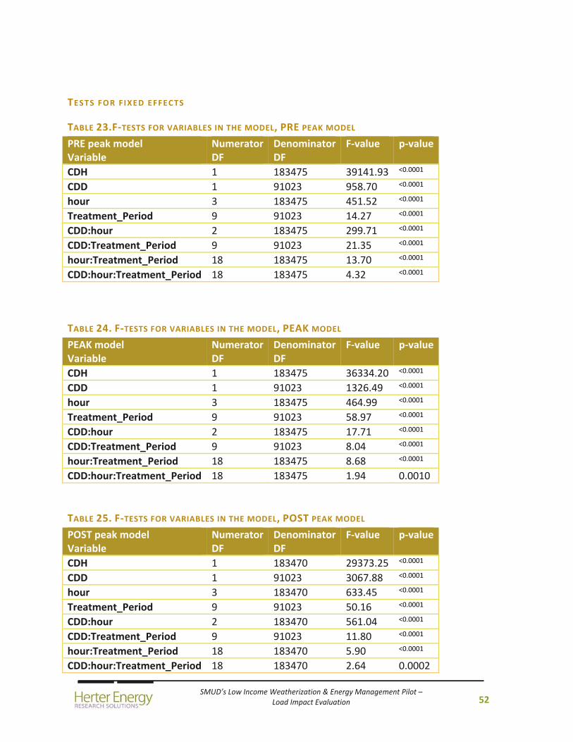
SMUD’s Low Income Weatherization & Energy Management Pilot – Load Impact Evaluation
52
TESTS FOR FIXED EFFECTS
TABLE 23.F‐TESTS FOR VARIABLES IN THE MODEL, PRE PEAK MODEL
PRE peak model Variable
NumeratorDF
DenominatorDF
F‐value p‐value
CDH 1 183475 39141.93 <0.0001
CDD 1 91023 958.70 <0.0001
hour 3 183475 451.52 <0.0001
Treatment_Period 9 91023 14.27 <0.0001
CDD:hour 2 183475 299.71 <0.0001
CDD:Treatment_Period 9 91023 21.35 <0.0001
hour:Treatment_Period 18 183475 13.70 <0.0001
CDD:hour:Treatment_Period 18 183475 4.32 <0.0001
TABLE 24. F‐TESTS FOR VARIABLES IN THE MODEL, PEAK MODEL
PEAK model Variable
NumeratorDF
DenominatorDF
F‐value p‐value
CDH 1 183475 36334.20 <0.0001
CDD 1 91023 1326.49 <0.0001
hour 3 183475 464.99 <0.0001
Treatment_Period 9 91023 58.97 <0.0001
CDD:hour 2 183475 17.71 <0.0001
CDD:Treatment_Period 9 91023 8.04 <0.0001
hour:Treatment_Period 18 183475 8.68 <0.0001
CDD:hour:Treatment_Period 18 183475 1.94 0.0010
TABLE 25. F‐TESTS FOR VARIABLES IN THE MODEL, POST PEAK MODEL
POST peak model Variable
NumeratorDF
DenominatorDF
F‐value p‐value
CDH 1 183470 29373.25 <0.0001
CDD 1 91023 3067.88 <0.0001
hour 3 183470 633.45 <0.0001
Treatment_Period 9 91023 50.16 <0.0001
CDD:hour 2 183470 561.04 <0.0001
CDD:Treatment_Period 9 91023 11.80 <0.0001
hour:Treatment_Period 18 183470 5.90 <0.0001
CDD:hour:Treatment_Period 18 183470 2.64 0.0002
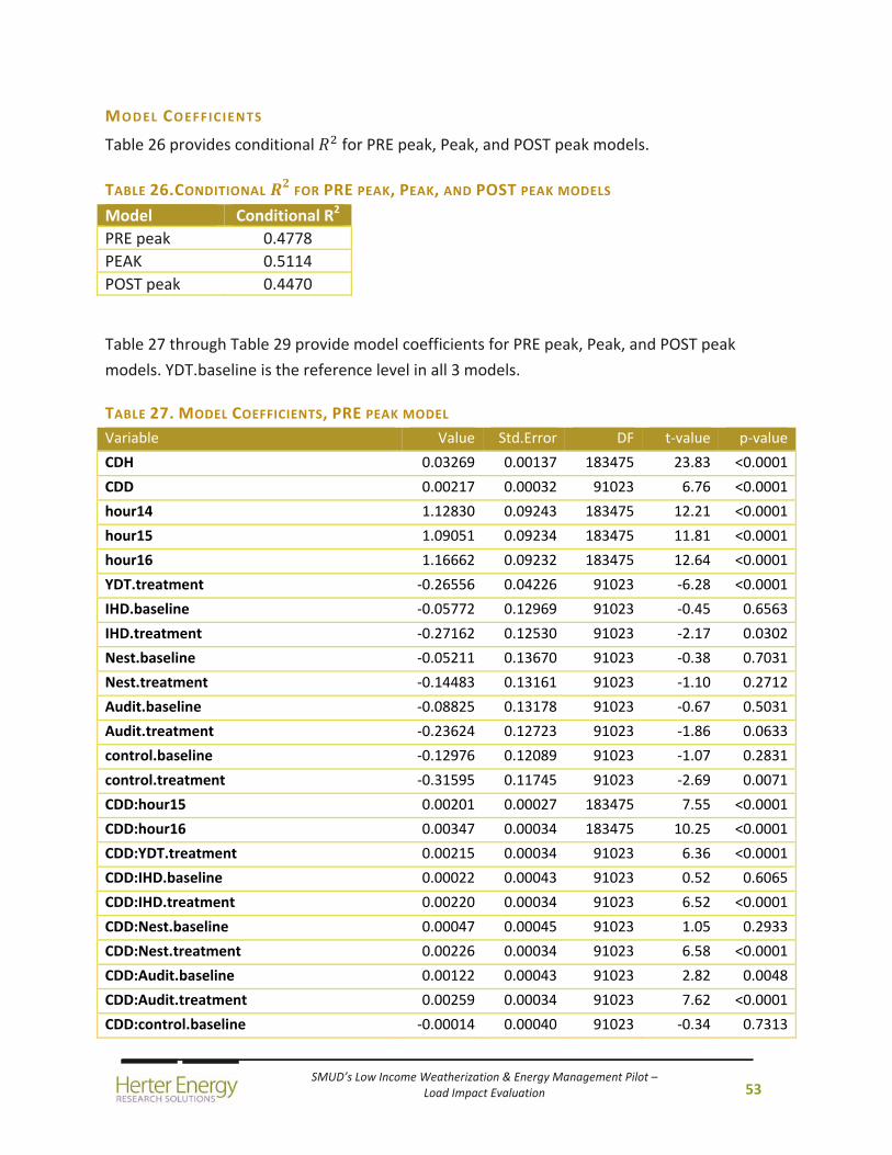
SMUD’s Low Income Weatherization & Energy Management Pilot – Load Impact Evaluation
53
MODEL COEFFIC IENTS
Table 26 provides conditional for PRE peak, Peak, and POST peak models.
TABLE 26.CONDITIONAL FOR PRE PEAK, PEAK, AND POST PEAK MODELS
Model Conditional R2
PRE peak 0.4778
PEAK 0.5114
POST peak 0.4470
Table 27 through Table 29 provide model coefficients for PRE peak, Peak, and POST peak
models. YDT.baseline is the reference level in all 3 models.
TABLE 27. MODEL COEFFICIENTS, PRE PEAK MODEL
Variable Value Std.Error DF t‐value p‐value
CDH 0.03269 0.00137 183475 23.83 <0.0001
CDD 0.00217 0.00032 91023 6.76 <0.0001
hour14 1.12830 0.09243 183475 12.21 <0.0001
hour15 1.09051 0.09234 183475 11.81 <0.0001
hour16 1.16662 0.09232 183475 12.64 <0.0001
YDT.treatment ‐0.26556 0.04226 91023 ‐6.28 <0.0001
IHD.baseline ‐0.05772 0.12969 91023 ‐0.45 0.6563
IHD.treatment ‐0.27162 0.12530 91023 ‐2.17 0.0302
Nest.baseline ‐0.05211 0.13670 91023 ‐0.38 0.7031
Nest.treatment ‐0.14483 0.13161 91023 ‐1.10 0.2712
Audit.baseline ‐0.08825 0.13178 91023 ‐0.67 0.5031
Audit.treatment ‐0.23624 0.12723 91023 ‐1.86 0.0633
control.baseline ‐0.12976 0.12089 91023 ‐1.07 0.2831
control.treatment ‐0.31595 0.11745 91023 ‐2.69 0.0071
CDD:hour15 0.00201 0.00027 183475 7.55 <0.0001
CDD:hour16 0.00347 0.00034 183475 10.25 <0.0001
CDD:YDT.treatment 0.00215 0.00034 91023 6.36 <0.0001
CDD:IHD.baseline 0.00022 0.00043 91023 0.52 0.6065
CDD:IHD.treatment 0.00220 0.00034 91023 6.52 <0.0001
CDD:Nest.baseline 0.00047 0.00045 91023 1.05 0.2933
CDD:Nest.treatment 0.00226 0.00034 91023 6.58 <0.0001
CDD:Audit.baseline 0.00122 0.00043 91023 2.82 0.0048
CDD:Audit.treatment 0.00259 0.00034 91023 7.62 <0.0001
CDD:control.baseline ‐0.00014 0.00040 91023 ‐0.34 0.7313
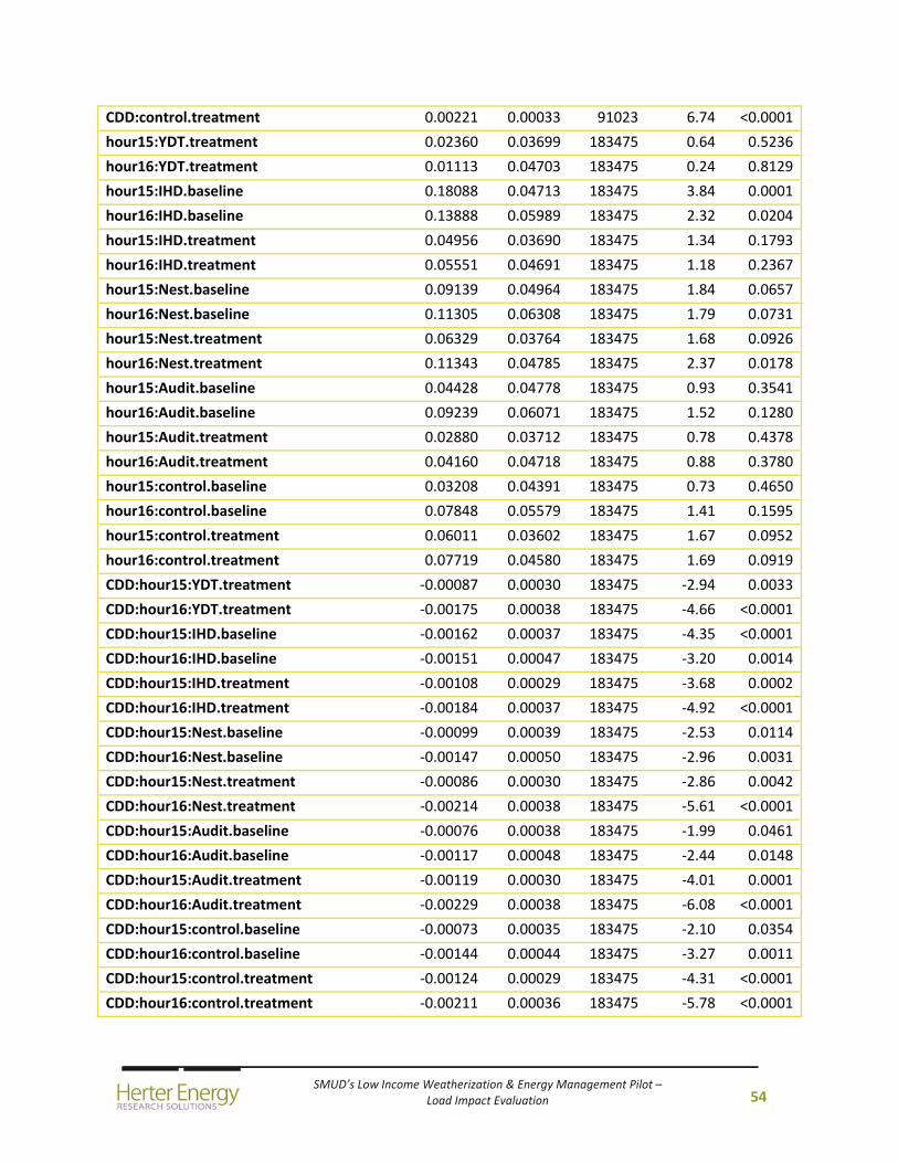
SMUD’s Low Income Weatherization & Energy Management Pilot – Load Impact Evaluation
54
CDD:control.treatment 0.00221 0.00033 91023 6.74 <0.0001
hour15:YDT.treatment 0.02360 0.03699 183475 0.64 0.5236
hour16:YDT.treatment 0.01113 0.04703 183475 0.24 0.8129
hour15:IHD.baseline 0.18088 0.04713 183475 3.84 0.0001
hour16:IHD.baseline 0.13888 0.05989 183475 2.32 0.0204
hour15:IHD.treatment 0.04956 0.03690 183475 1.34 0.1793
hour16:IHD.treatment 0.05551 0.04691 183475 1.18 0.2367
hour15:Nest.baseline 0.09139 0.04964 183475 1.84 0.0657
hour16:Nest.baseline 0.11305 0.06308 183475 1.79 0.0731
hour15:Nest.treatment 0.06329 0.03764 183475 1.68 0.0926
hour16:Nest.treatment 0.11343 0.04785 183475 2.37 0.0178
hour15:Audit.baseline 0.04428 0.04778 183475 0.93 0.3541
hour16:Audit.baseline 0.09239 0.06071 183475 1.52 0.1280
hour15:Audit.treatment 0.02880 0.03712 183475 0.78 0.4378
hour16:Audit.treatment 0.04160 0.04718 183475 0.88 0.3780
hour15:control.baseline 0.03208 0.04391 183475 0.73 0.4650
hour16:control.baseline 0.07848 0.05579 183475 1.41 0.1595
hour15:control.treatment 0.06011 0.03602 183475 1.67 0.0952
hour16:control.treatment 0.07719 0.04580 183475 1.69 0.0919
CDD:hour15:YDT.treatment ‐0.00087 0.00030 183475 ‐2.94 0.0033
CDD:hour16:YDT.treatment ‐0.00175 0.00038 183475 ‐4.66 <0.0001
CDD:hour15:IHD.baseline ‐0.00162 0.00037 183475 ‐4.35 <0.0001
CDD:hour16:IHD.baseline ‐0.00151 0.00047 183475 ‐3.20 0.0014
CDD:hour15:IHD.treatment ‐0.00108 0.00029 183475 ‐3.68 0.0002
CDD:hour16:IHD.treatment ‐0.00184 0.00037 183475 ‐4.92 <0.0001
CDD:hour15:Nest.baseline ‐0.00099 0.00039 183475 ‐2.53 0.0114
CDD:hour16:Nest.baseline ‐0.00147 0.00050 183475 ‐2.96 0.0031
CDD:hour15:Nest.treatment ‐0.00086 0.00030 183475 ‐2.86 0.0042
CDD:hour16:Nest.treatment ‐0.00214 0.00038 183475 ‐5.61 <0.0001
CDD:hour15:Audit.baseline ‐0.00076 0.00038 183475 ‐1.99 0.0461
CDD:hour16:Audit.baseline ‐0.00117 0.00048 183475 ‐2.44 0.0148
CDD:hour15:Audit.treatment ‐0.00119 0.00030 183475 ‐4.01 0.0001
CDD:hour16:Audit.treatment ‐0.00229 0.00038 183475 ‐6.08 <0.0001
CDD:hour15:control.baseline ‐0.00073 0.00035 183475 ‐2.10 0.0354
CDD:hour16:control.baseline ‐0.00144 0.00044 183475 ‐3.27 0.0011
CDD:hour15:control.treatment ‐0.00124 0.00029 183475 ‐4.31 <0.0001
CDD:hour16:control.treatment ‐0.00211 0.00036 183475 ‐5.78 <0.0001
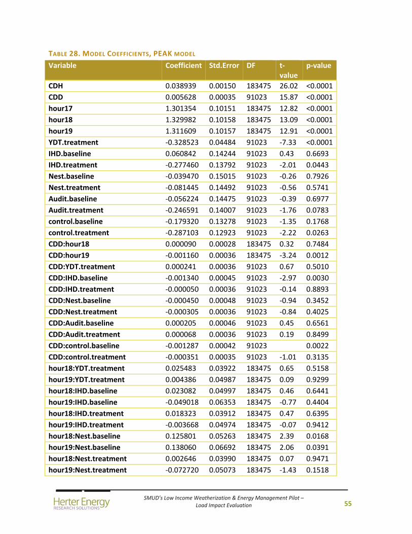
SMUD’s Low Income Weatherization & Energy Management Pilot – Load Impact Evaluation
55
TABLE 28. MODEL COEFFICIENTS, PEAK MODEL
Variable Coefficient Std.Error DF t‐value
p‐value
CDH 0.038939 0.00150 183475 26.02 <0.0001
CDD 0.005628 0.00035 91023 15.87 <0.0001
hour17 1.301354 0.10151 183475 12.82 <0.0001
hour18 1.329982 0.10158 183475 13.09 <0.0001
hour19 1.311609 0.10157 183475 12.91 <0.0001
YDT.treatment ‐0.328523 0.04484 91023 ‐7.33 <0.0001
IHD.baseline 0.060842 0.14244 91023 0.43 0.6693
IHD.treatment ‐0.277460 0.13792 91023 ‐2.01 0.0443
Nest.baseline ‐0.039470 0.15015 91023 ‐0.26 0.7926
Nest.treatment ‐0.081445 0.14492 91023 ‐0.56 0.5741
Audit.baseline ‐0.056224 0.14475 91023 ‐0.39 0.6977
Audit.treatment ‐0.246591 0.14007 91023 ‐1.76 0.0783
control.baseline ‐0.179320 0.13278 91023 ‐1.35 0.1768
control.treatment ‐0.287103 0.12923 91023 ‐2.22 0.0263
CDD:hour18 0.000090 0.00028 183475 0.32 0.7484
CDD:hour19 ‐0.001160 0.00036 183475 ‐3.24 0.0012
CDD:YDT.treatment 0.000241 0.00036 91023 0.67 0.5010
CDD:IHD.baseline ‐0.001340 0.00045 91023 ‐2.97 0.0030
CDD:IHD.treatment ‐0.000050 0.00036 91023 ‐0.14 0.8893
CDD:Nest.baseline ‐0.000450 0.00048 91023 ‐0.94 0.3452
CDD:Nest.treatment ‐0.000305 0.00036 91023 ‐0.84 0.4025
CDD:Audit.baseline 0.000205 0.00046 91023 0.45 0.6561
CDD:Audit.treatment 0.000068 0.00036 91023 0.19 0.8499
CDD:control.baseline ‐0.001287 0.00042 91023 0.0022
CDD:control.treatment ‐0.000351 0.00035 91023 ‐1.01 0.3135
hour18:YDT.treatment 0.025483 0.03922 183475 0.65 0.5158
hour19:YDT.treatment 0.004386 0.04987 183475 0.09 0.9299
hour18:IHD.baseline 0.023082 0.04997 183475 0.46 0.6441
hour19:IHD.baseline ‐0.049018 0.06353 183475 ‐0.77 0.4404
hour18:IHD.treatment 0.018323 0.03912 183475 0.47 0.6395
hour19:IHD.treatment ‐0.003668 0.04974 183475 ‐0.07 0.9412
hour18:Nest.baseline 0.125801 0.05263 183475 2.39 0.0168
hour19:Nest.baseline 0.138060 0.06692 183475 2.06 0.0391
hour18:Nest.treatment 0.002646 0.03990 183475 0.07 0.9471
hour19:Nest.treatment ‐0.072720 0.05073 183475 ‐1.43 0.1518
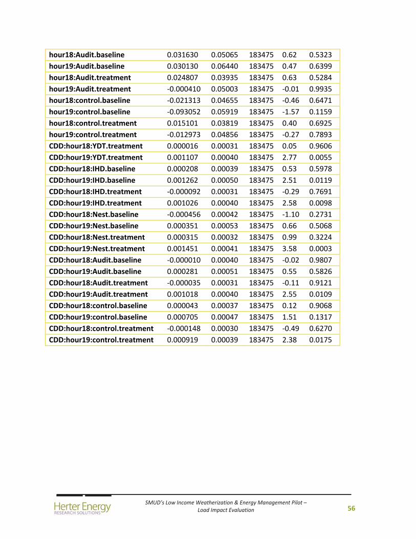
SMUD’s Low Income Weatherization & Energy Management Pilot – Load Impact Evaluation
56
hour18:Audit.baseline 0.031630 0.05065 183475 0.62 0.5323
hour19:Audit.baseline 0.030130 0.06440 183475 0.47 0.6399
hour18:Audit.treatment 0.024807 0.03935 183475 0.63 0.5284
hour19:Audit.treatment ‐0.000410 0.05003 183475 ‐0.01 0.9935
hour18:control.baseline ‐0.021313 0.04655 183475 ‐0.46 0.6471
hour19:control.baseline ‐0.093052 0.05919 183475 ‐1.57 0.1159
hour18:control.treatment 0.015101 0.03819 183475 0.40 0.6925
hour19:control.treatment ‐0.012973 0.04856 183475 ‐0.27 0.7893
CDD:hour18:YDT.treatment 0.000016 0.00031 183475 0.05 0.9606
CDD:hour19:YDT.treatment 0.001107 0.00040 183475 2.77 0.0055
CDD:hour18:IHD.baseline 0.000208 0.00039 183475 0.53 0.5978
CDD:hour19:IHD.baseline 0.001262 0.00050 183475 2.51 0.0119
CDD:hour18:IHD.treatment ‐0.000092 0.00031 183475 ‐0.29 0.7691
CDD:hour19:IHD.treatment 0.001026 0.00040 183475 2.58 0.0098
CDD:hour18:Nest.baseline ‐0.000456 0.00042 183475 ‐1.10 0.2731
CDD:hour19:Nest.baseline 0.000351 0.00053 183475 0.66 0.5068
CDD:hour18:Nest.treatment 0.000315 0.00032 183475 0.99 0.3224
CDD:hour19:Nest.treatment 0.001451 0.00041 183475 3.58 0.0003
CDD:hour18:Audit.baseline ‐0.000010 0.00040 183475 ‐0.02 0.9807
CDD:hour19:Audit.baseline 0.000281 0.00051 183475 0.55 0.5826
CDD:hour18:Audit.treatment ‐0.000035 0.00031 183475 ‐0.11 0.9121
CDD:hour19:Audit.treatment 0.001018 0.00040 183475 2.55 0.0109
CDD:hour18:control.baseline 0.000043 0.00037 183475 0.12 0.9068
CDD:hour19:control.baseline 0.000705 0.00047 183475 1.51 0.1317
CDD:hour18:control.treatment ‐0.000148 0.00030 183475 ‐0.49 0.6270
CDD:hour19:control.treatment 0.000919 0.00039 183475 2.38 0.0175
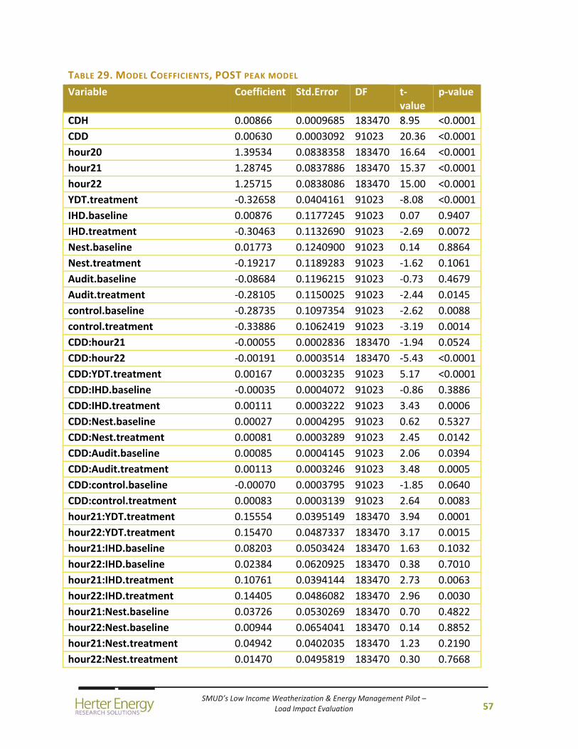
SMUD’s Low Income Weatherization & Energy Management Pilot – Load Impact Evaluation
57
TABLE 29. MODEL COEFFICIENTS, POST PEAK MODEL
Variable Coefficient Std.Error DF t‐value
p‐value
CDH 0.00866 0.0009685 183470 8.95 <0.0001
CDD 0.00630 0.0003092 91023 20.36 <0.0001
hour20 1.39534 0.0838358 183470 16.64 <0.0001
hour21 1.28745 0.0837886 183470 15.37 <0.0001
hour22 1.25715 0.0838086 183470 15.00 <0.0001
YDT.treatment ‐0.32658 0.0404161 91023 ‐8.08 <0.0001
IHD.baseline 0.00876 0.1177245 91023 0.07 0.9407
IHD.treatment ‐0.30463 0.1132690 91023 ‐2.69 0.0072
Nest.baseline 0.01773 0.1240900 91023 0.14 0.8864
Nest.treatment ‐0.19217 0.1189283 91023 ‐1.62 0.1061
Audit.baseline ‐0.08684 0.1196215 91023 ‐0.73 0.4679
Audit.treatment ‐0.28105 0.1150025 91023 ‐2.44 0.0145
control.baseline ‐0.28735 0.1097354 91023 ‐2.62 0.0088
control.treatment ‐0.33886 0.1062419 91023 ‐3.19 0.0014
CDD:hour21 ‐0.00055 0.0002836 183470 ‐1.94 0.0524
CDD:hour22 ‐0.00191 0.0003514 183470 ‐5.43 <0.0001
CDD:YDT.treatment 0.00167 0.0003235 91023 5.17 <0.0001
CDD:IHD.baseline ‐0.00035 0.0004072 91023 ‐0.86 0.3886
CDD:IHD.treatment 0.00111 0.0003222 91023 3.43 0.0006
CDD:Nest.baseline 0.00027 0.0004295 91023 0.62 0.5327
CDD:Nest.treatment 0.00081 0.0003289 91023 2.45 0.0142
CDD:Audit.baseline 0.00085 0.0004145 91023 2.06 0.0394
CDD:Audit.treatment 0.00113 0.0003246 91023 3.48 0.0005
CDD:control.baseline ‐0.00070 0.0003795 91023 ‐1.85 0.0640
CDD:control.treatment 0.00083 0.0003139 91023 2.64 0.0083
hour21:YDT.treatment 0.15554 0.0395149 183470 3.94 0.0001
hour22:YDT.treatment 0.15470 0.0487337 183470 3.17 0.0015
hour21:IHD.baseline 0.08203 0.0503424 183470 1.63 0.1032
hour22:IHD.baseline 0.02384 0.0620925 183470 0.38 0.7010
hour21:IHD.treatment 0.10761 0.0394144 183470 2.73 0.0063
hour22:IHD.treatment 0.14405 0.0486082 183470 2.96 0.0030
hour21:Nest.baseline 0.03726 0.0530269 183470 0.70 0.4822
hour22:Nest.baseline 0.00944 0.0654041 183470 0.14 0.8852
hour21:Nest.treatment 0.04942 0.0402035 183470 1.23 0.2190
hour22:Nest.treatment 0.01470 0.0495819 183470 0.30 0.7668
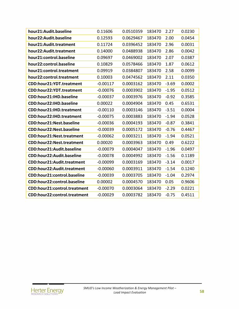
SMUD’s Low Income Weatherization & Energy Management Pilot – Load Impact Evaluation
58
hour21:Audit.baseline 0.11606 0.0510359 183470 2.27 0.0230
hour22:Audit.baseline 0.12593 0.0629467 183470 2.00 0.0454
hour21:Audit.treatment 0.11724 0.0396452 183470 2.96 0.0031
hour22:Audit.treatment 0.14000 0.0488938 183470 2.86 0.0042
hour21:control.baseline 0.09697 0.0469002 183470 2.07 0.0387
hour22:control.baseline 0.10829 0.0578466 183470 1.87 0.0612
hour21:control.treatment 0.09919 0.0384807 183470 2.58 0.0099
hour22:control.treatment 0.10003 0.0474562 183470 2.11 0.0350
CDD:hour21:YDT.treatment ‐0.00117 0.0003162 183470 ‐3.69 0.0002
CDD:hour22:YDT.treatment ‐0.00076 0.0003902 183470 ‐1.95 0.0512
CDD:hour21:IHD.baseline ‐0.00037 0.0003976 183470 ‐0.92 0.3585
CDD:hour22:IHD.baseline 0.00022 0.0004904 183470 0.45 0.6531
CDD:hour21:IHD.treatment ‐0.00110 0.0003146 183470 ‐3.51 0.0004
CDD:hour22:IHD.treatment ‐0.00075 0.0003883 183470 ‐1.94 0.0528
CDD:hour21:Nest.baseline ‐0.00036 0.0004193 183470 ‐0.87 0.3841
CDD:hour22:Nest.baseline ‐0.00039 0.0005172 183470 ‐0.76 0.4467
CDD:hour21:Nest.treatment ‐0.00062 0.0003211 183470 ‐1.94 0.0521
CDD:hour22:Nest.treatment 0.00020 0.0003963 183470 0.49 0.6222
CDD:hour21:Audit.baseline ‐0.00079 0.0004047 183470 ‐1.96 0.0497
CDD:hour22:Audit.baseline ‐0.00078 0.0004992 183470 ‐1.56 0.1189
CDD:hour21:Audit.treatment ‐0.00099 0.0003169 183470 ‐3.14 0.0017
CDD:hour22:Audit.treatment ‐0.00060 0.0003911 183470 ‐1.54 0.1240
CDD:hour21:control.baseline ‐0.00039 0.0003705 183470 ‐1.04 0.2974
CDD:hour22:control.baseline 0.00002 0.0004570 183470 0.05 0.9606
CDD:hour21:control.treatment ‐0.00070 0.0003064 183470 ‐2.29 0.0221
CDD:hour22:control.treatment ‐0.00029 0.0003782 183470 ‐0.75 0.4511
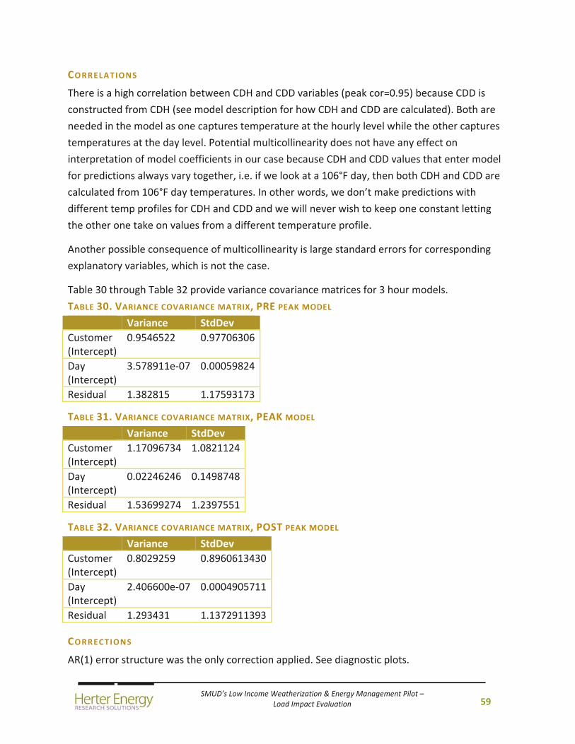
SMUD’s Low Income Weatherization & Energy Management Pilot – Load Impact Evaluation
59
CORRELATIONS
There is a high correlation between CDH and CDD variables (peak cor=0.95) because CDD is
constructed from CDH (see model description for how CDH and CDD are calculated). Both are
needed in the model as one captures temperature at the hourly level while the other captures
temperatures at the day level. Potential multicollinearity does not have any effect on
interpretation of model coefficients in our case because CDH and CDD values that enter model
for predictions always vary together, i.e. if we look at a 106°F day, then both CDH and CDD are
calculated from 106°F day temperatures. In other words, we don’t make predictions with
different temp profiles for CDH and CDD and we will never wish to keep one constant letting
the other one take on values from a different temperature profile.
Another possible consequence of multicollinearity is large standard errors for corresponding
explanatory variables, which is not the case.
Table 30 through Table 32 provide variance covariance matrices for 3 hour models.
TABLE 30. VARIANCE COVARIANCE MATRIX, PRE PEAK MODEL
Variance StdDev
Customer (Intercept)
0.9546522 0.97706306
Day (Intercept)
3.578911e‐07 0.00059824
Residual 1.382815 1.17593173
TABLE 31. VARIANCE COVARIANCE MATRIX, PEAK MODEL
Variance StdDev
Customer (Intercept)
1.17096734 1.0821124
Day (Intercept)
0.02246246 0.1498748
Residual 1.53699274 1.2397551
TABLE 32. VARIANCE COVARIANCE MATRIX, POST PEAK MODEL
Variance StdDev
Customer (Intercept)
0.8029259 0.8960613430
Day (Intercept)
2.406600e‐07 0.0004905711
Residual 1.293431 1.1372911393
CORRECTIONS
AR(1) error structure was the only correction applied. See diagnostic plots.
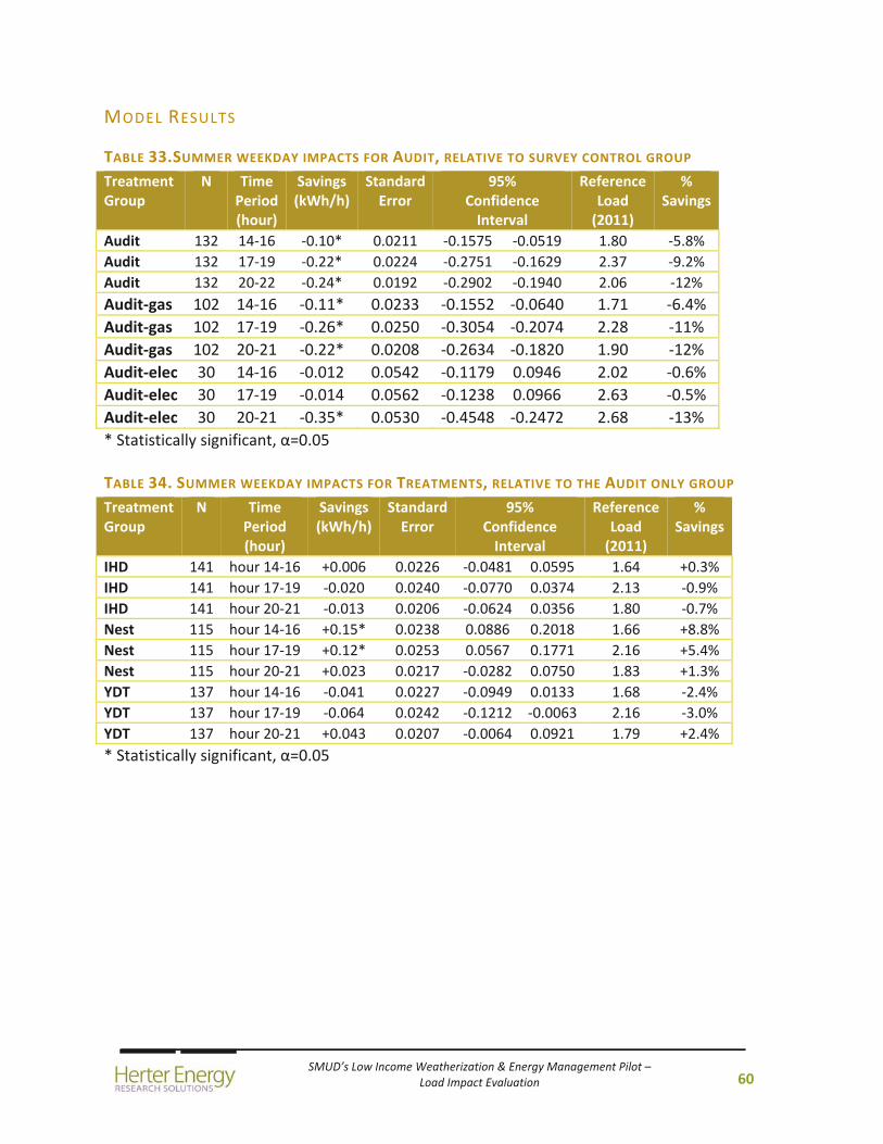
SMUD’s Low Income Weatherization & Energy Management Pilot – Load Impact Evaluation
60
MODEL RESULTS
TABLE 33.SUMMER WEEKDAY IMPACTS FOR AUDIT, RELATIVE TO SURVEY CONTROL GROUP
Treatment Group
N Time Period (hour)
Savings (kWh/h)
StandardError
95% Confidence Interval
Reference Load (2011)
% Savings
Audit 132 14‐16 ‐0.10* 0.0211 ‐0.1575 ‐0.0519 1.80 ‐5.8%
Audit 132 17‐19 ‐0.22* 0.0224 ‐0.2751 ‐0.1629 2.37 ‐9.2%
Audit 132 20‐22 ‐0.24* 0.0192 ‐0.2902 ‐0.1940 2.06 ‐12%
Audit‐gas 102 14‐16 ‐0.11* 0.0233 ‐0.1552 ‐0.0640 1.71 ‐6.4%
Audit‐gas 102 17‐19 ‐0.26* 0.0250 ‐0.3054 ‐0.2074 2.28 ‐11%
Audit‐gas 102 20‐21 ‐0.22* 0.0208 ‐0.2634 ‐0.1820 1.90 ‐12%
Audit‐elec 30 14‐16 ‐0.012 0.0542 ‐0.1179 0.0946 2.02 ‐0.6%
Audit‐elec 30 17‐19 ‐0.014 0.0562 ‐0.1238 0.0966 2.63 ‐0.5%
Audit‐elec 30 20‐21 ‐0.35* 0.0530 ‐0.4548 ‐0.2472 2.68 ‐13%
* Statistically significant, α=0.05
TABLE 34. SUMMER WEEKDAY IMPACTS FOR TREATMENTS, RELATIVE TO THE AUDIT ONLY GROUP
Treatment Group
N Time Period (hour)
Savings (kWh/h)
StandardError
95% Confidence Interval
Reference Load (2011)
% Savings
IHD 141 hour 14‐16 +0.006 0.0226 ‐0.0481 0.0595 1.64 +0.3%
IHD 141 hour 17‐19 ‐0.020 0.0240 ‐0.0770 0.0374 2.13 ‐0.9%
IHD 141 hour 20‐21 ‐0.013 0.0206 ‐0.0624 0.0356 1.80 ‐0.7%
Nest 115 hour 14‐16 +0.15* 0.0238 0.0886 0.2018 1.66 +8.8%
Nest 115 hour 17‐19 +0.12* 0.0253 0.0567 0.1771 2.16 +5.4%
Nest 115 hour 20‐21 +0.023 0.0217 ‐0.0282 0.0750 1.83 +1.3%
YDT 137 hour 14‐16 ‐0.041 0.0227 ‐0.0949 0.0133 1.68 ‐2.4%
YDT 137 hour 17‐19 ‐0.064 0.0242 ‐0.1212 ‐0.0063 2.16 ‐3.0%
YDT 137 hour 20‐21 +0.043 0.0207 ‐0.0064 0.0921 1.79 +2.4%
* Statistically significant, α=0.05
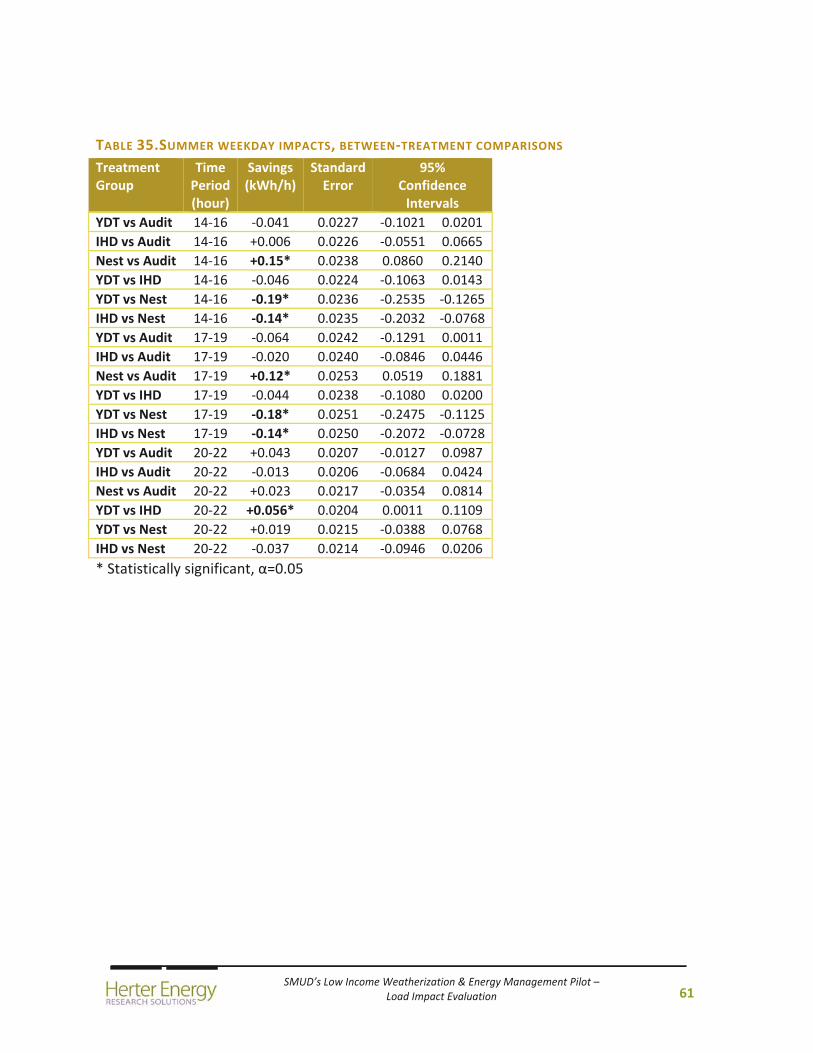
SMUD’s Low Income Weatherization & Energy Management Pilot – Load Impact Evaluation
61
TABLE 35.SUMMER WEEKDAY IMPACTS, BETWEEN‐TREATMENT COMPARISONS
Treatment Group
Time Period (hour)
Savings (kWh/h)
StandardError
95% Confidence Intervals
YDT vs Audit 14‐16 ‐0.041 0.0227 ‐0.1021 0.0201
IHD vs Audit 14‐16 +0.006 0.0226 ‐0.0551 0.0665
Nest vs Audit 14‐16 +0.15* 0.0238 0.0860 0.2140
YDT vs IHD 14‐16 ‐0.046 0.0224 ‐0.1063 0.0143
YDT vs Nest 14‐16 ‐0.19* 0.0236 ‐0.2535 ‐0.1265
IHD vs Nest 14‐16 ‐0.14* 0.0235 ‐0.2032 ‐0.0768
YDT vs Audit 17‐19 ‐0.064 0.0242 ‐0.1291 0.0011
IHD vs Audit 17‐19 ‐0.020 0.0240 ‐0.0846 0.0446
Nest vs Audit 17‐19 +0.12* 0.0253 0.0519 0.1881
YDT vs IHD 17‐19 ‐0.044 0.0238 ‐0.1080 0.0200
YDT vs Nest 17‐19 ‐0.18* 0.0251 ‐0.2475 ‐0.1125
IHD vs Nest 17‐19 ‐0.14* 0.0250 ‐0.2072 ‐0.0728
YDT vs Audit 20‐22 +0.043 0.0207 ‐0.0127 0.0987
IHD vs Audit 20‐22 ‐0.013 0.0206 ‐0.0684 0.0424
Nest vs Audit 20‐22 +0.023 0.0217 ‐0.0354 0.0814
YDT vs IHD 20‐22 +0.056* 0.0204 0.0011 0.1109
YDT vs Nest 20‐22 +0.019 0.0215 ‐0.0388 0.0768
IHD vs Nest 20‐22 ‐0.037 0.0214 ‐0.0946 0.0206
* Statistically significant, α=0.05
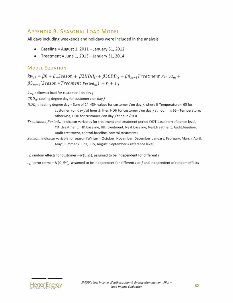
SMUD’s Low Income Weatherization & Energy Management Pilot – Load Impact Evaluation
62
APPENDIX B. SEASONAL LOAD MODEL All days including weekends and holidays were included in the analysis
Baseline = August 1, 2011 – January 31, 2012
Treatment = June 1, 2013 – January 31, 2014
MODEL EQUATION
0 1 2 3 4 _
5 ∗ _
: kilowatt load for customer on day
: cooling degree day for customer on day
: heating degree day = Sum of 24 HDH values for customer on day , where If Temperature < 65 for
customer on day at hour , then HDH for customer on day at hour � is 65 ‐ Temperature;
otherwise, HDH for customer on day at hour is 0
_ : indicator variables for treatment and treatment period (YDT.baseline=reference level,
YDT.treatment, IHD.baseline, IHD.treatment, Nest.baseline, Nest.treatment, Audit.baseline,
Audit.treatment, control.baseline, control.treatment)
: indicator variable for season (Winter = October, November, December, January, February, March, April,
May; Summer = June, July, August, September = reference level)
: random effects for customer ~ 0, , assumed to be independent for different
: error terms ~ 0, , assumed to be independent for different or and independent of random effects
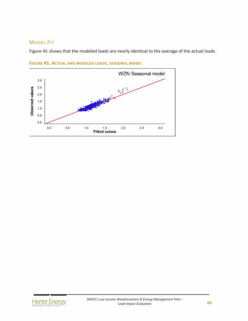
SMUD’s Low Income Weatherization & Energy Management Pilot – Load Impact Evaluation
63
MODEL FIT
Figure 45 shows that the modeled loads are nearly identical to the average of the actual loads.
FIGURE 45. ACTUAL AND MODELED LOADS, SEASONAL MODEL
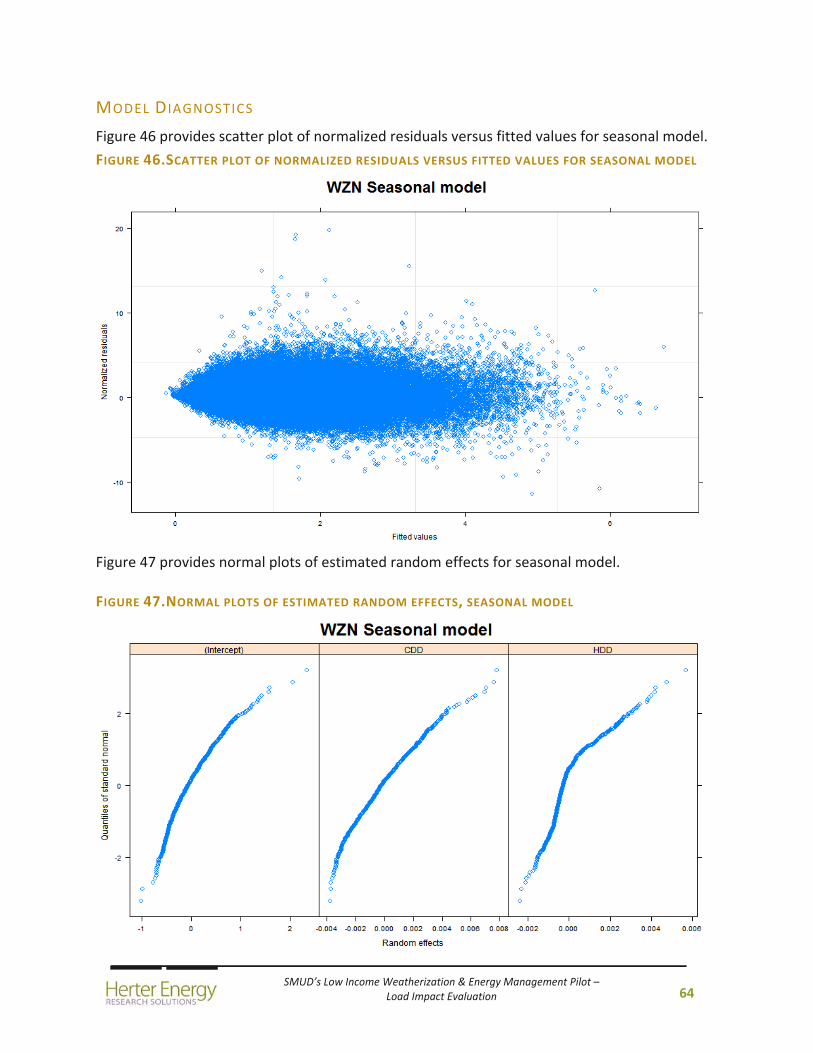
SMUD’s Low Income Weatherization & Energy Management Pilot – Load Impact Evaluation
64
MODEL DIAGNOSTICS
Figure 46 provides scatter plot of normalized residuals versus fitted values for seasonal model.
FIGURE 46.SCATTER PLOT OF NORMALIZED RESIDUALS VERSUS FITTED VALUES FOR SEASONAL MODEL
Figure 47 provides normal plots of estimated random effects for seasonal model.
FIGURE 47.NORMAL PLOTS OF ESTIMATED RANDOM EFFECTS, SEASONAL MODEL
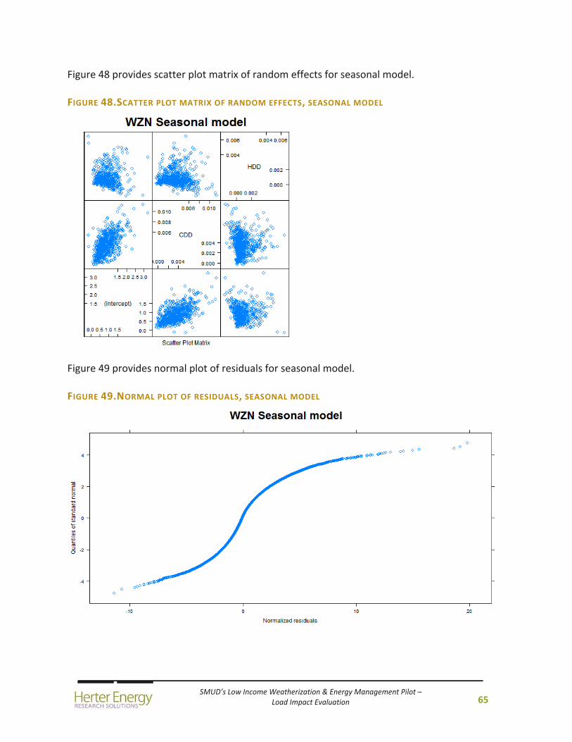
SMUD’s Low Income Weatherization & Energy Management Pilot – Load Impact Evaluation
65
Figure 48 provides scatter plot matrix of random effects for seasonal model.
FIGURE 48.SCATTER PLOT MATRIX OF RANDOM EFFECTS, SEASONAL MODEL
Figure 49 provides normal plot of residuals for seasonal model.
FIGURE 49.NORMAL PLOT OF RESIDUALS, SEASONAL MODEL
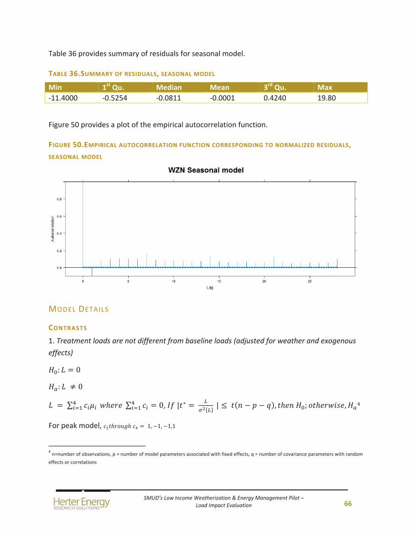
SMUD’s Low Income Weatherization & Energy Management Pilot – Load Impact Evaluation
66
Table 36 provides summary of residuals for seasonal model.
TABLE 36.SUMMARY OF RESIDUALS, SEASONAL MODEL
Min 1st Qu. Median Mean 3rd Qu. Max
‐11.4000 ‐0.5254 ‐0.0811 ‐0.0001 0.4240 19.80
Figure 50 provides a plot of the empirical autocorrelation function.
FIGURE 50.EMPIRICAL AUTOCORRELATION FUNCTION CORRESPONDING TO NORMALIZED RESIDUALS,
SEASONAL MODEL
MODEL DETAILS
CONTRASTS
1. Treatment loads are not different from baseline loads (adjusted for weather and exogenous
effects)
: 0
: 0
∑ ∑ 0, | ∗ | , ; , 4
For peak model, 1, 1, 1,1
4 n=number of observations, p = number of model parameters associated with fixed effects, q = number of covariance parameters with random
effects or correlations

SMUD’s Low Income Weatherization & Energy Management Pilot – Load Impact Evaluation
67
2. Treatment type has no effect on impacts (adjusted for weather and exogenous effects)
Same as in 1 above but different set of means.
CONTRASTS EXAMPLES
YDT summer impact relative to baseline (adjusted for weather and exogenous effects), and
comparing YDT and IHD treatments (adjusted for weather and pretreatment differences)
1. Treatment loads are not different from baseline loads (adjusted for weather and exogenous
effects)
. . . . . . . . . . . .
2. Treatment type has no effect on impacts (adjusted for weather and exogenous effects)
. . . . . . . . . . . .
Notes:
′ are estimated using regression coefficients with the temperature profile of interest –
average temp summer 2013.
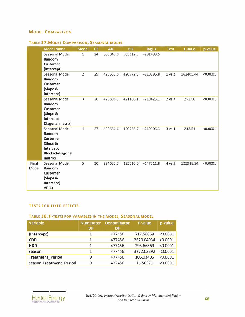
SMUD’s Low Income Weatherization & Energy Management Pilot – Load Impact Evaluation
68
MODEL COMPARISON
TABLE 37.MODEL COMPARISON, SEASONAL MODEL
Model Name Model DF AIC BIC logLik Test L.Ratio p‐value
Seasonal Model Random Customer (Intercept)
1 24 583047.0 583312.9 ‐291499.5
Seasonal Model Random Customer (Slope & Intercept)
2 29 420651.6 420972.8 ‐210296.8 1 vs 2 162405.44 <0.0001
Seasonal Model Random Customer (Slope & Intercept Diagonal matrix)
3 26 420898.1 421186.1 ‐210423.1 2 vs 3 252.56 <0.0001
Seasonal Model Random Customer (Slope & Intercept Blocked‐diagonal matrix)
4 27 420666.6 420965.7 ‐210306.3 3 vs 4 233.51 <0.0001
Final Model
Seasonal Model Random Customer (Slope & Intercept) AR(1)
5 30 294683.7 295016.0 ‐147311.8 4 vs 5 125988.94 <0.0001
TESTS FOR FIXED EFFECTS
TABLE 38. F‐TESTS FOR VARIABLES IN THE MODEL, SEASONAL MODEL
Variable NumeratorDF
DenominatorDF
F‐value p‐value
(Intercept) 1 477456 717.56059 <0.0001
CDD 1 477456 2620.04934 <0.0001
HDD 1 477456 295.66869 <0.0001
season 1 477456 3272.02292 <0.0001
Treatment_Period 9 477456 106.03405 <0.0001
season:Treatment_Period 9 477456 16.56321 <0.0001
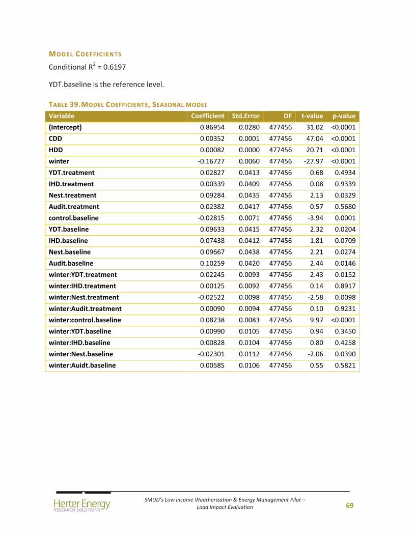
SMUD’s Low Income Weatherization & Energy Management Pilot – Load Impact Evaluation
69
MODEL COEFFIC IENTS
Conditional R2 = 0.6197
YDT.baseline is the reference level.
TABLE 39.MODEL COEFFICIENTS, SEASONAL MODEL
Variable Coefficient Std.Error DF t‐value p‐value
(Intercept) 0.86954 0.0280 477456 31.02 <0.0001
CDD 0.00352 0.0001 477456 47.04 <0.0001
HDD 0.00082 0.0000 477456 20.71 <0.0001
winter ‐0.16727 0.0060 477456 ‐27.97 <0.0001
YDT.treatment 0.02827 0.0413 477456 0.68 0.4934
IHD.treatment 0.00339 0.0409 477456 0.08 0.9339
Nest.treatment 0.09284 0.0435 477456 2.13 0.0329
Audit.treatment 0.02382 0.0417 477456 0.57 0.5680
control.baseline ‐0.02815 0.0071 477456 ‐3.94 0.0001
YDT.baseline 0.09633 0.0415 477456 2.32 0.0204
IHD.baseline 0.07438 0.0412 477456 1.81 0.0709
Nest.baseline 0.09667 0.0438 477456 2.21 0.0274
Audit.baseline 0.10259 0.0420 477456 2.44 0.0146
winter:YDT.treatment 0.02245 0.0093 477456 2.43 0.0152
winter:IHD.treatment 0.00125 0.0092 477456 0.14 0.8917
winter:Nest.treatment ‐0.02522 0.0098 477456 ‐2.58 0.0098
winter:Audit.treatment 0.00090 0.0094 477456 0.10 0.9231
winter:control.baseline 0.08238 0.0083 477456 9.97 <0.0001
winter:YDT.baseline 0.00990 0.0105 477456 0.94 0.3450
winter:IHD.baseline 0.00828 0.0104 477456 0.80 0.4258
winter:Nest.baseline ‐0.02301 0.0112 477456 ‐2.06 0.0390
winter:Auidt.baseline 0.00585 0.0106 477456 0.55 0.5821
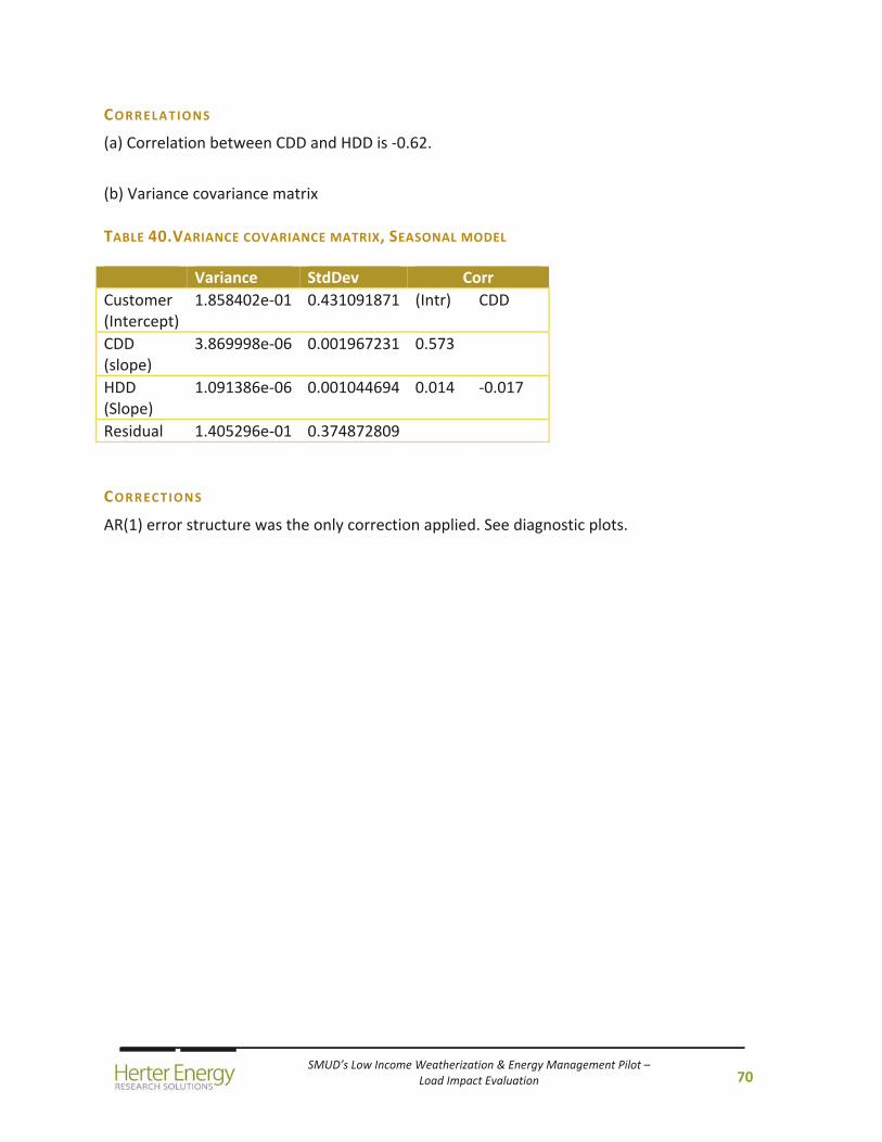
SMUD’s Low Income Weatherization & Energy Management Pilot – Load Impact Evaluation
70
CORRELATIONS
(a) Correlation between CDD and HDD is ‐0.62.
(b) Variance covariance matrix
TABLE 40.VARIANCE COVARIANCE MATRIX, SEASONAL MODEL
Variance StdDev Corr
Customer (Intercept)
1.858402e‐01 0.431091871 (Intr) CDD
CDD (slope)
3.869998e‐06 0.001967231 0.573
HDD (Slope)
1.091386e‐06 0.001044694 0.014 ‐0.017
Residual 1.405296e‐01 0.374872809
CORRECTIONS
AR(1) error structure was the only correction applied. See diagnostic plots.
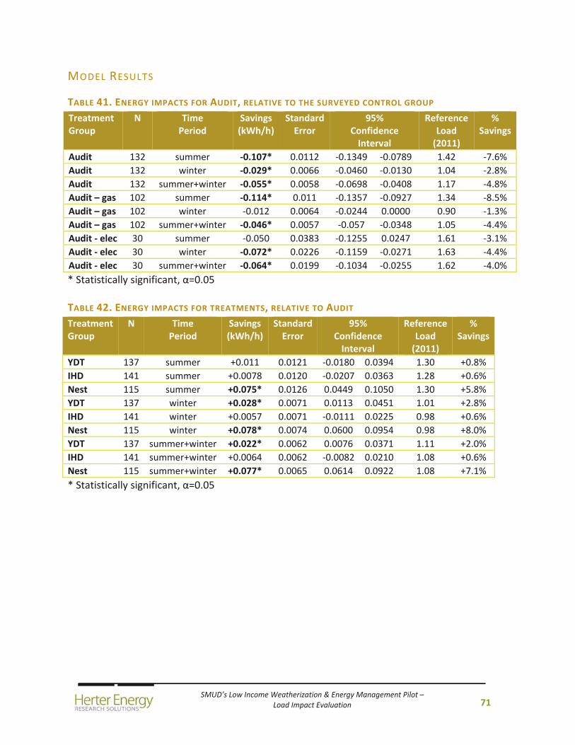
SMUD’s Low Income Weatherization & Energy Management Pilot – Load Impact Evaluation
71
MODEL RESULTS
TABLE 41. ENERGY IMPACTS FOR AUDIT, RELATIVE TO THE SURVEYED CONTROL GROUP
Treatment Group
N Time Period
Savings (kWh/h)
StandardError
95% Confidence Interval
ReferenceLoad (2011)
% Savings
Audit 132 summer ‐0.107* 0.0112 ‐0.1349 ‐0.0789 1.42 ‐7.6%
Audit 132 winter ‐0.029* 0.0066 ‐0.0460 ‐0.0130 1.04 ‐2.8%
Audit 132 summer+winter ‐0.055* 0.0058 ‐0.0698 ‐0.0408 1.17 ‐4.8%
Audit – gas 102 summer ‐0.114* 0.011 ‐0.1357 ‐0.0927 1.34 ‐8.5%
Audit – gas 102 winter ‐0.012 0.0064 ‐0.0244 0.0000 0.90 ‐1.3%
Audit – gas 102 summer+winter ‐0.046* 0.0057 ‐0.057 ‐0.0348 1.05 ‐4.4%
Audit ‐ elec 30 summer ‐0.050 0.0383 ‐0.1255 0.0247 1.61 ‐3.1%
Audit ‐ elec 30 winter ‐0.072* 0.0226 ‐0.1159 ‐0.0271 1.63 ‐4.4%
Audit ‐ elec 30 summer+winter ‐0.064* 0.0199 ‐0.1034 ‐0.0255 1.62 ‐4.0%
* Statistically significant, α=0.05
TABLE 42. ENERGY IMPACTS FOR TREATMENTS, RELATIVE TO AUDIT
Treatment Group
N Time Period
Savings (kWh/h)
StandardError
95% Confidence Interval
Reference Load (2011)
% Savings
YDT 137 summer +0.011 0.0121 ‐0.0180 0.0394 1.30 +0.8%
IHD 141 summer +0.0078 0.0120 ‐0.0207 0.0363 1.28 +0.6%
Nest 115 summer +0.075* 0.0126 0.0449 0.1050 1.30 +5.8%
YDT 137 winter +0.028* 0.0071 0.0113 0.0451 1.01 +2.8%
IHD 141 winter +0.0057 0.0071 ‐0.0111 0.0225 0.98 +0.6%
Nest 115 winter +0.078* 0.0074 0.0600 0.0954 0.98 +8.0%
YDT 137 summer+winter +0.022* 0.0062 0.0076 0.0371 1.11 +2.0%
IHD 141 summer+winter +0.0064 0.0062 ‐0.0082 0.0210 1.08 +0.6%
Nest 115 summer+winter +0.077* 0.0065 0.0614 0.0922 1.08 +7.1%
* Statistically significant, α=0.05
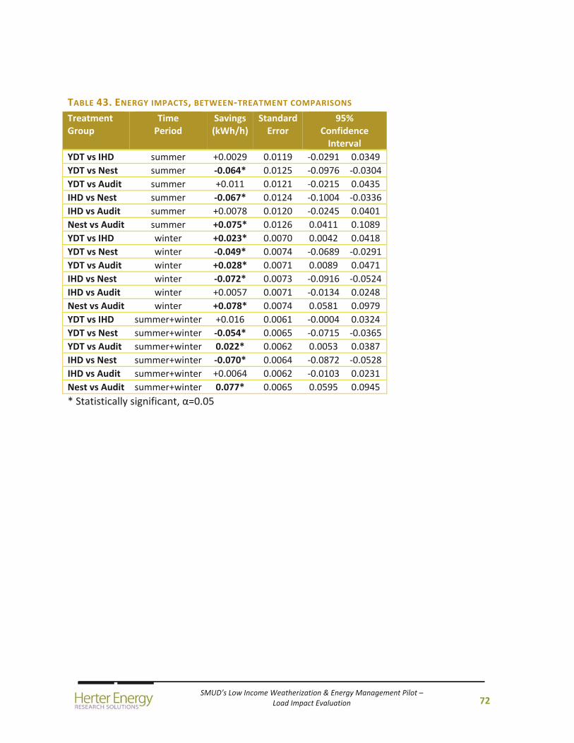
SMUD’s Low Income Weatherization & Energy Management Pilot – Load Impact Evaluation
72
TABLE 43. ENERGY IMPACTS, BETWEEN‐TREATMENT COMPARISONS
Treatment Group
Time Period
Savings (kWh/h)
StandardError
95% Confidence Interval
YDT vs IHD summer +0.0029 0.0119 ‐0.0291 0.0349
YDT vs Nest summer ‐0.064* 0.0125 ‐0.0976 ‐0.0304
YDT vs Audit summer +0.011 0.0121 ‐0.0215 0.0435
IHD vs Nest summer ‐0.067* 0.0124 ‐0.1004 ‐0.0336
IHD vs Audit summer +0.0078 0.0120 ‐0.0245 0.0401
Nest vs Audit summer +0.075* 0.0126 0.0411 0.1089
YDT vs IHD winter +0.023* 0.0070 0.0042 0.0418
YDT vs Nest winter ‐0.049* 0.0074 ‐0.0689 ‐0.0291
YDT vs Audit winter +0.028* 0.0071 0.0089 0.0471
IHD vs Nest winter ‐0.072* 0.0073 ‐0.0916 ‐0.0524
IHD vs Audit winter +0.0057 0.0071 ‐0.0134 0.0248
Nest vs Audit winter +0.078* 0.0074 0.0581 0.0979
YDT vs IHD summer+winter +0.016 0.0061 ‐0.0004 0.0324
YDT vs Nest summer+winter ‐0.054* 0.0065 ‐0.0715 ‐0.0365
YDT vs Audit summer+winter 0.022* 0.0062 0.0053 0.0387
IHD vs Nest summer+winter ‐0.070* 0.0064 ‐0.0872 ‐0.0528
IHD vs Audit summer+winter +0.0064 0.0062 ‐0.0103 0.0231
Nest vs Audit summer+winter 0.077* 0.0065 0.0595 0.0945
* Statistically significant, α=0.05
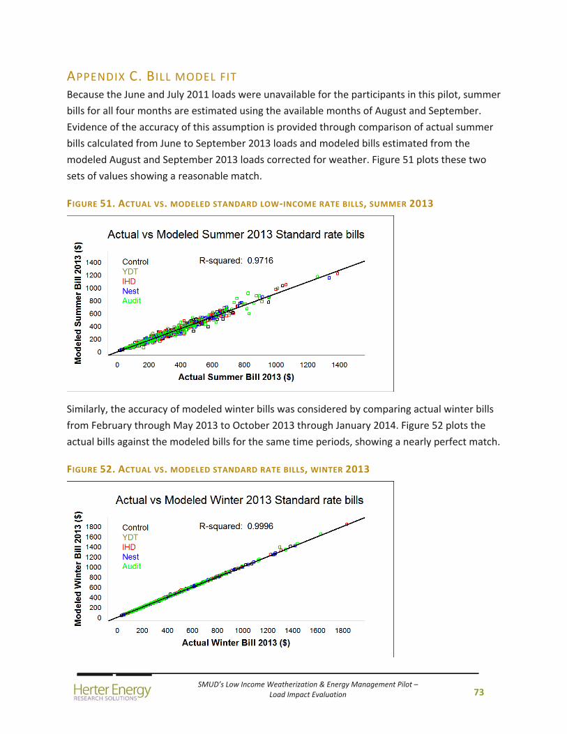
SMUD’s Low Income Weatherization & Energy Management Pilot – Load Impact Evaluation
73
APPENDIX C. BILL MODEL FIT Because the June and July 2011 loads were unavailable for the participants in this pilot, summer
bills for all four months are estimated using the available months of August and September.
Evidence of the accuracy of this assumption is provided through comparison of actual summer
bills calculated from June to September 2013 loads and modeled bills estimated from the
modeled August and September 2013 loads corrected for weather. Figure 51 plots these two
sets of values showing a reasonable match.
FIGURE 51. ACTUAL VS. MODELED STANDARD LOW‐INCOME RATE BILLS, SUMMER 2013
Similarly, the accuracy of modeled winter bills was considered by comparing actual winter bills
from February through May 2013 to October 2013 through January 2014. Figure 52 plots the
actual bills against the modeled bills for the same time periods, showing a nearly perfect match.
FIGURE 52. ACTUAL VS. MODELED STANDARD RATE BILLS, WINTER 2013
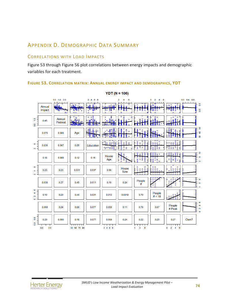
SMUD’s Low Income Weatherization & Energy Management Pilot – Load Impact Evaluation
74
APPENDIX D. DEMOGRAPHIC DATA SUMMARY
CORRELATIONS WITH LOAD IMPACTS
Figure 53 through Figure 56 plot correlations between energy impacts and demographic
variables for each treatment.
FIGURE 53. CORRELATION MATRIX: ANNUAL ENERGY IMPACT AND DEMOGRAPHICS, YDT
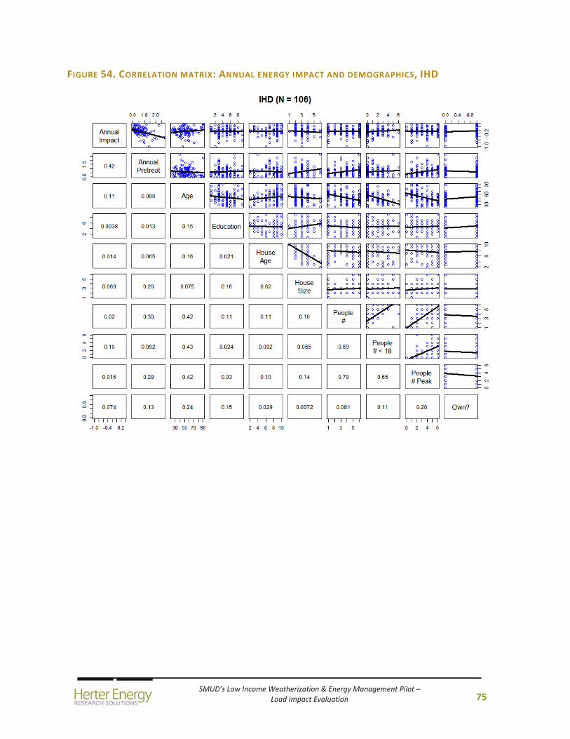
SMUD’s Low Income Weatherization & Energy Management Pilot – Load Impact Evaluation
75
FIGURE 54. CORRELATION MATRIX: ANNUAL ENERGY IMPACT AND DEMOGRAPHICS, IHD
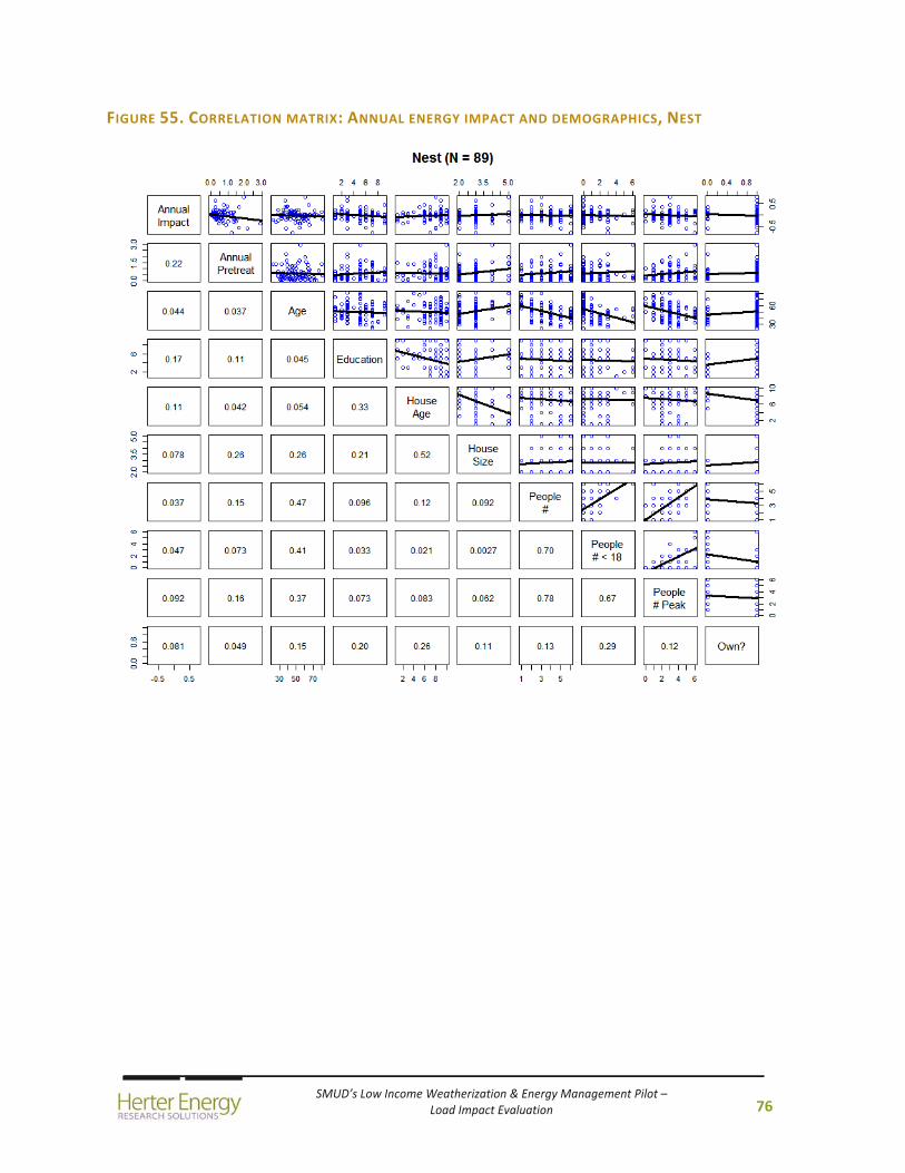
SMUD’s Low Income Weatherization & Energy Management Pilot – Load Impact Evaluation
76
FIGURE 55. CORRELATION MATRIX: ANNUAL ENERGY IMPACT AND DEMOGRAPHICS, NEST
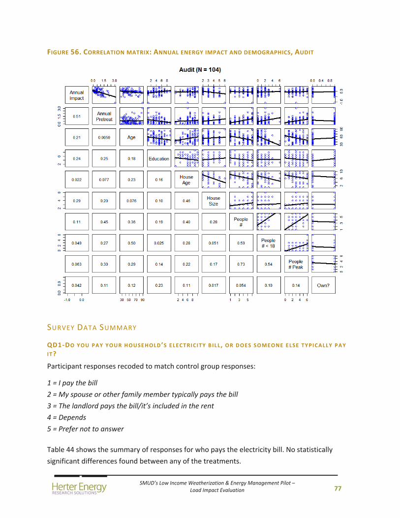
SMUD’s Low Income Weatherization & Energy Management Pilot – Load Impact Evaluation
77
FIGURE 56. CORRELATION MATRIX: ANNUAL ENERGY IMPACT AND DEMOGRAPHICS, AUDIT
SURVEY DATA SUMMARY
QD1 ‐DO YOU PAY YOUR HOUSEHOLD’S ELECTRICITY BILL , OR DOES SOMEONE ELSE TYPICALLY PAY
IT?
Participant responses recoded to match control group responses:
1 = I pay the bill
2 = My spouse or other family member typically pays the bill
3 = The landlord pays the bill/it’s included in the rent
4 = Depends
5 = Prefer not to answer
Table 44 shows the summary of responses for who pays the electricity bill. No statistically
significant differences found between any of the treatments.
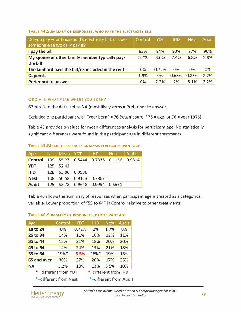
SMUD’s Low Income Weatherization & Energy Management Pilot – Load Impact Evaluation
78
TABLE 44.SUMMARY OF RESPONSES, WHO PAYS THE ELECTRICITY BILL
Do you pay your household's electricity bill, or does someone else typically pay it?
Control YDT IHD Nest Audit
I pay the bill 92% 94% 90% 87% 90%
My spouse or other family member typically pays the bill
5.7% 3.6% 7.4% 6.8% 5.8%
The landlord pays the bill/its included in the rent 0% 0.72% 0% 0% 0%
Depends 1.9% 0% 0.68% 0.85% 2.2%
Prefer not to answer 0% 2.2% 2% 5.1% 2.2%
QD2 – IN WHAT YEAR WHERE YOU BORN?
67 zero’s in the data, set to NA (most likely zeros = Prefer not to answer).
Excluded one participant with “year born” = 76 (wasn’t sure if 76 = age, or 76 = year 1976).
Table 45 provides p‐values for mean differences analysis for participant age. No statistically
significant differences were found in the participant age in different treatments.
TABLE 45.MEAN DIFFERENCES ANALYSIS FOR PARTICIPANT AGE
Age N Mean YDT IHD Nest Audit
Control 199 55.27 0.5444 0.7336 0.1156 0.9314
YDT 125 52.42
IHD 128 53.00 0.9986
Nest 108 50.58 0.9113 0.7867
Audit 125 53.78 0.9648 0.9954 0.5661
Table 46 shows the summary of responses when participant age is treated as a categorical
variable. Lower proportion of “55 to 64” in Control relative to other treatments.
TABLE 46.SUMMARY OF RESPONSES, PARTICIPANT AGE
Age Control YDT IHD Nest Audit
18 to 24 0% 0.72% 2% 1.7% 0%
25 to 34 14% 11% 10% 13% 11%
35 to 44 18% 21% 18% 20% 20%
45 to 54 14% 24% 19% 21% 18%
55 to 64 19%* 6.5% 18%* 19% 16%
65 and over 30% 27% 20% 17% 25%
NA 5.2% 10% 13% 8.5% 10%
*= different from YDT *=different from IHD
*=different from Nest *=different from Audit
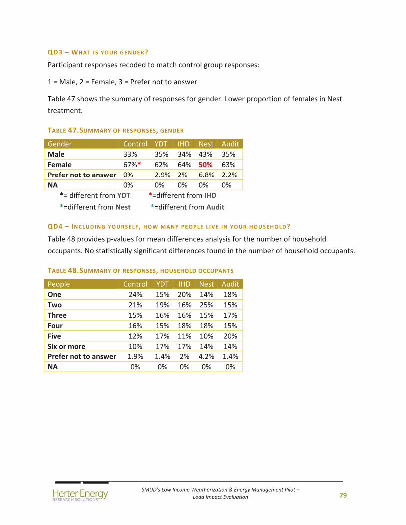
SMUD’s Low Income Weatherization & Energy Management Pilot – Load Impact Evaluation
79
QD3 – WHAT I S YOUR GENDER?
Participant responses recoded to match control group responses:
1 = Male, 2 = Female, 3 = Prefer not to answer
Table 47 shows the summary of responses for gender. Lower proportion of females in Nest
treatment.
TABLE 47.SUMMARY OF RESPONSES, GENDER
Gender Control YDT IHD Nest Audit
Male 33% 35% 34% 43% 35%
Female 67%* 62% 64% 50% 63%
Prefer not to answer 0% 2.9% 2% 6.8% 2.2%
NA 0% 0% 0% 0% 0%
*= different from YDT *=different from IHD
*=different from Nest *=different from Audit
QD4 – INCLUDING YOURSELF, HOW MANY PEOPLE L IVE IN YOUR HOUSEHOLD?
Table 48 provides p‐values for mean differences analysis for the number of household
occupants. No statistically significant differences found in the number of household occupants.
TABLE 48.SUMMARY OF RESPONSES, HOUSEHOLD OCCUPANTS
People Control YDT IHD Nest Audit
One 24% 15% 20% 14% 18%
Two 21% 19% 16% 25% 15%
Three 15% 16% 16% 15% 17%
Four 16% 15% 18% 18% 15%
Five 12% 17% 11% 10% 20%
Six or more 10% 17% 17% 14% 14%
Prefer not to answer 1.9% 1.4% 2% 4.2% 1.4%
NA 0% 0% 0% 0% 0%
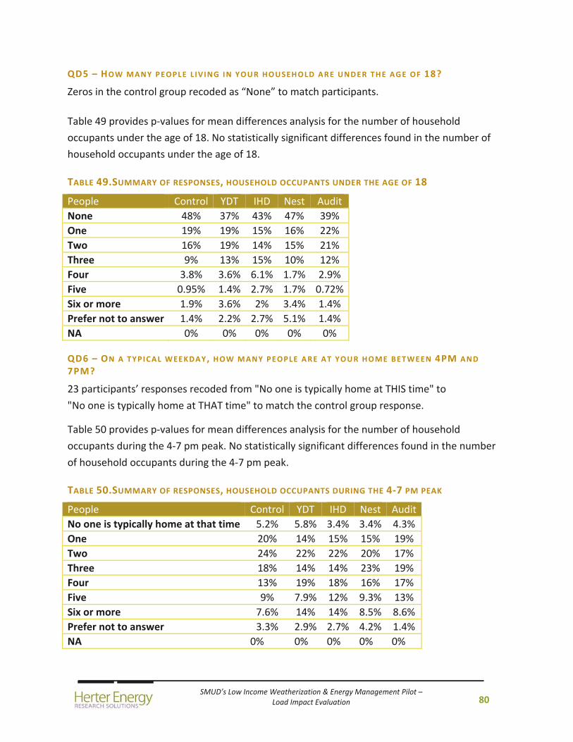
SMUD’s Low Income Weatherization & Energy Management Pilot – Load Impact Evaluation
80
QD5 – HOW MANY PEOPLE L IV ING IN YOUR HOUSEHOLD ARE UNDER THE AGE OF 18?
Zeros in the control group recoded as “None” to match participants.
Table 49 provides p‐values for mean differences analysis for the number of household
occupants under the age of 18. No statistically significant differences found in the number of
household occupants under the age of 18.
TABLE 49.SUMMARY OF RESPONSES, HOUSEHOLD OCCUPANTS UNDER THE AGE OF 18
People Control YDT IHD Nest Audit
None 48% 37% 43% 47% 39%
One 19% 19% 15% 16% 22%
Two 16% 19% 14% 15% 21%
Three 9% 13% 15% 10% 12%
Four 3.8% 3.6% 6.1% 1.7% 2.9%
Five 0.95% 1.4% 2.7% 1.7% 0.72%
Six or more 1.9% 3.6% 2% 3.4% 1.4%
Prefer not to answer 1.4% 2.2% 2.7% 5.1% 1.4%
NA 0% 0% 0% 0% 0%
QD6 – ON A TYPICAL WEEKDAY, HOW MANY PEOPLE ARE AT YOUR HOME BETWEEN 4PM AND
7PM?
23 participants’ responses recoded from "No one is typically home at THIS time" to
"No one is typically home at THAT time" to match the control group response.
Table 50 provides p‐values for mean differences analysis for the number of household
occupants during the 4‐7 pm peak. No statistically significant differences found in the number
of household occupants during the 4‐7 pm peak.
TABLE 50.SUMMARY OF RESPONSES, HOUSEHOLD OCCUPANTS DURING THE 4‐7 PM PEAK
People Control YDT IHD Nest Audit
No one is typically home at that time 5.2% 5.8% 3.4% 3.4% 4.3%
One 20% 14% 15% 15% 19%
Two 24% 22% 22% 20% 17%
Three 18% 14% 14% 23% 19%
Four 13% 19% 18% 16% 17%
Five 9% 7.9% 12% 9.3% 13%
Six or more 7.6% 14% 14% 8.5% 8.6%
Prefer not to answer 3.3% 2.9% 2.7% 4.2% 1.4%
NA 0% 0% 0% 0% 0%

SMUD’s Low Income Weatherization & Energy Management Pilot – Load Impact Evaluation
81
QD7 – DO YOU OWN OR RENT YOUR HOME?
Table 51 shows the summary of responses for whether participants own or rent their homes.
Lower proportion of owners in Control group relative to Nest treatment. Higher proportion of
renters in Control group relative to YDT and Nest treatments. Higher proportion of renters in
IHD relative to Nest treatment.
TABLE 51.SUMMARY OF RESPONSES, OWN/RENT
Own/Rent Control YDT IHD Nest Audit
Own 61%* 75% 65% 81% 70%
Rent 37%** 22% 33%* 16% 27%
Prefer not to answer 1.9% 3.6% 2% 3.4% 2.9%
NA 0% 0% 0% 0% 0%
*= different from YDT *=different from IHD
*=different from Nest *=different from Audit
QD8 – WHAT ETHNIC GROUP DO YOU CONSIDER YOURSELF A PART OF OR FEEL CLOSEST TO?
1 “No opinion/Not Sure” response in the participants group was changed to “Not sure” to
match control group.
5 “Other heritage” responses in the participants group were changed to “Other” to match
control group.
13 "Asian – Korean, Japanese, Chinese, Vietnamese, Filipino…” responses were changed to
“Asian‐Korean, Japanese, Chinese, Vietnamese, Filipino, or ot”.
4 “Mixed Heritage” responses were change to “Mixed heritage” responses.
Table 52 shows the summary of responses for ethnic group. Higher proportion of
“Caucasian/White” and lower proportion of “Asian” and “Pacific Islander” in Control group
relative to YDT.
TABLE 52.SUMMARY OF RESPONSES, ETHNIC GROUP
Ethnic group Control YDT IHD Nest Audit
Caucasian/White 45%* 27% 34% 42% 33%
Latino/Hispanic/Mexican 14% 13% 17% 19% 18%
African‐American/Black 16% 19% 18% 9.3% 12%
Native American Indian or Alaskan Native 1.4% 2.2% 0.68% 0.85% 3.6%
Asian‐Korean, Japanese, Chinese, Vietnamese, Filipino, or other Asian
6.7%* 19% 14% 12% 14%
Pacific Islander 0.48%* 7.2% 5.4% 1.7% 5%
Mixed heritage 1.9% 3.6% 4.7% 5.1% 3.6%
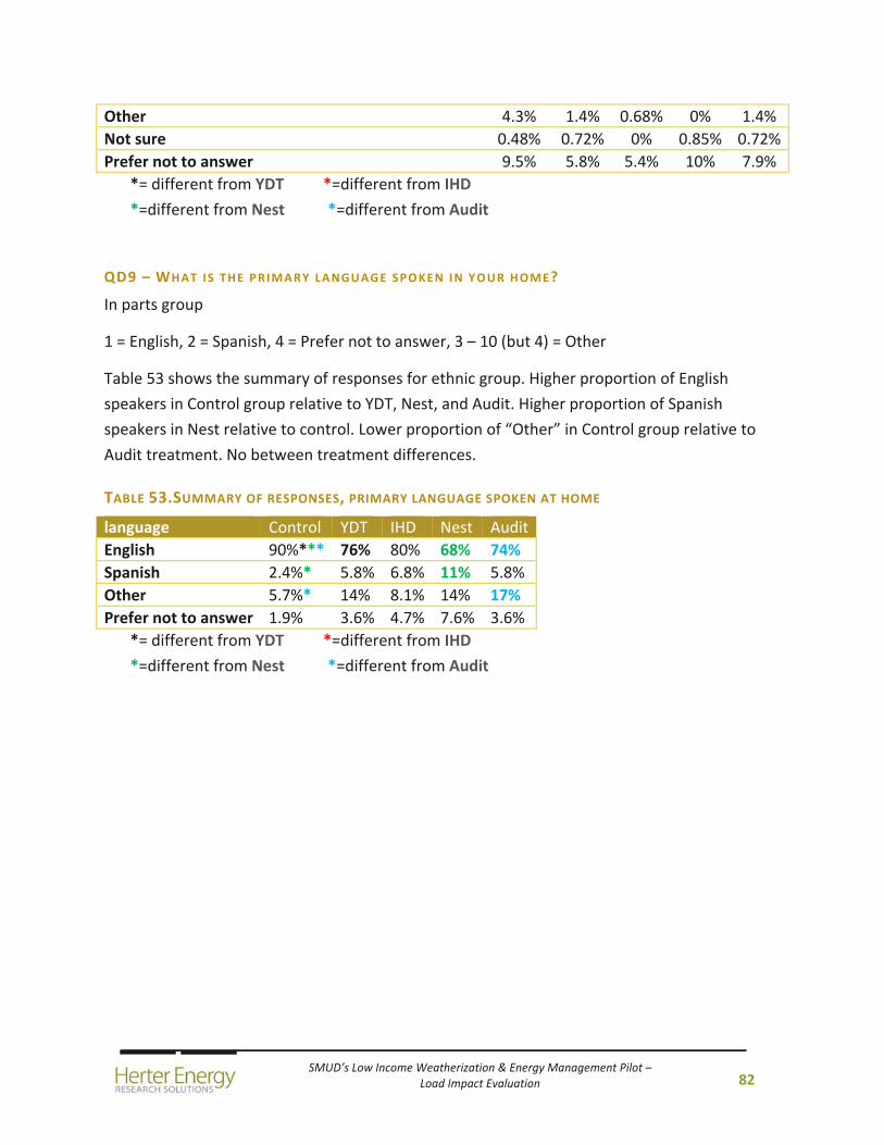
SMUD’s Low Income Weatherization & Energy Management Pilot – Load Impact Evaluation
82
Other 4.3% 1.4% 0.68% 0% 1.4%
Not sure 0.48% 0.72% 0% 0.85% 0.72%
Prefer not to answer 9.5% 5.8% 5.4% 10% 7.9%
*= different from YDT *=different from IHD
*=different from Nest *=different from Audit
QD9 – WHAT I S THE PRIMARY LANGUAGE SPOKEN IN YOUR HOME?
In parts group
1 = English, 2 = Spanish, 4 = Prefer not to answer, 3 – 10 (but 4) = Other
Table 53 shows the summary of responses for ethnic group. Higher proportion of English
speakers in Control group relative to YDT, Nest, and Audit. Higher proportion of Spanish
speakers in Nest relative to control. Lower proportion of “Other” in Control group relative to
Audit treatment. No between treatment differences.
TABLE 53.SUMMARY OF RESPONSES, PRIMARY LANGUAGE SPOKEN AT HOME
language Control YDT IHD Nest Audit
English 90%*** 76% 80% 68% 74%
Spanish 2.4%* 5.8% 6.8% 11% 5.8%
Other 5.7%* 14% 8.1% 14% 17%
Prefer not to answer 1.9% 3.6% 4.7% 7.6% 3.6%
*= different from YDT *=different from IHD
*=different from Nest *=different from Audit

SMUD’s Low Income Weatherization & Energy Management Pilot – Load Impact Evaluation
83
QD10 – WHAT IS THE LAST GRADE OR LEVEL YOU COMPLETED IN SCHOOL?
6 “Graduate, professional, doctorate degree (DDS, DVM, JD...)”
were changed to “Graduate, professional, doctorate degree”.
Table 54 shows the summary of responses when participant education is treated as a
categorical variable. No significant differences found.
TABLE 54.SUMMARY OF RESPONSES, PARTICIPANT EDUCATION
What is the last grade or level you completed in school?
Control YDT IHD Nest Audit
Elementary (8 or fewer years) 2.4% 2.2% 4.1% 5.9% 7.2%
Some high school (9 to 11 years) 6.2% 7.2% 4.7% 7.6% 5%
High school graduate (12 years) 31% 27% 22% 23% 22%
Technical / Vocational school 1.9% 3.6% 8.1% 0.85% 7.2%
Some college 25% 27% 24% 18% 21%
College graduate (2 year degree) 13% 9.4% 9.5% 10% 12%
College graduate (4 year degree) 13% 13% 14% 17% 14%
Some graduate school 0% 2.2% 2% 1.7% 3.6%
Graduate, professional, doctorate degree 2.9% 1.4% 2.7% 5.9% 2.9%
Prefer not to answer 3.8% 7.9% 8.8% 10% 6.5%
NA 0% 0% 0% 0% 0%
Ranked education level from 1 to 9. Prefer not to answer = NA
Table 55 provides p‐values for mean differences analysis for participant education. No
statistically significant differences were found in the participant education in different
treatments.
TABLE 55.MEAN DIFFERENCES ANALYSIS FOR PARTICIPANT EDUCATION
Education N Mean YDT IHD Nest Audit
Control 202 4.58 0.99999 0.9689 0.9183 0.9980
YDT 128 4.57
IHD 134 4.72 0.9732
Nest 106 4.77 0.9301 0.9994
Audit 130 4.65 0.9979 0.9983 0.9869
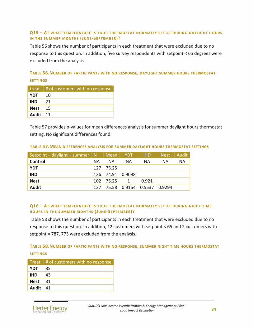
SMUD’s Low Income Weatherization & Energy Management Pilot – Load Impact Evaluation
84
Q15 – AT WHAT TEMPERATURE I S YOUR THERMOSTAT NORMALLY SET AT DURING DAYLIGHT HOURS
IN THE SUMMER MONTHS (JUNE‐SEPTEMBER)?
Table 56 shows the number of participants in each treatment that were excluded due to no
response to this question. In addition, five survey respondents with setpoint < 65 degrees were
excluded from the analysis.
TABLE 56.NUMBER OF PARTICIPANTS WITH NO RESPONSE, DAYLIGHT SUMMER HOURS THERMOSTAT
SETTINGS
treat # of customers with no response
YDT 10
IHD 21
Nest 15
Audit 11
Table 57 provides p‐values for mean differences analysis for summer daylight hours thermostat
setting. No significant differences found.
TABLE 57.MEAN DIFFERENCES ANALYSIS FOR SUMMER DAYLIGHT HOURS THERMOSTAT SETTINGS
Setpoint – daylight – summer N Mean YDT IHD Nest Audit
Control NA NA NA NA NA NA
YDT 127 75.25
IHD 126 74.91 0.9098
Nest 102 75.25 1 0.921
Audit 127 75.58 0.9154 0.5537 0.9294
Q16 – AT WHAT TEMPERATURE I S YOUR THERMOSTAT NORMALLY SET AT DURING NIGHT TIME
HOURS IN THE SUMMER MONTHS (JUNE‐SEPTEMBER)?
Table 58 shows the number of participants in each treatment that were excluded due to no
response to this question. In addition, 12 customers with setpoint < 65 and 2 customers with
setpoint = 787, 773 were excluded from the analysis.
TABLE 58.NUMBER OF PARTICIPANTS WITH NO RESPONSE, SUMMER NIGHT TIME HOURS THERMOSTAT
SETTINGS
Treat # of customers with no response
YDT 35
IHD 43
Nest 31
Audit 41
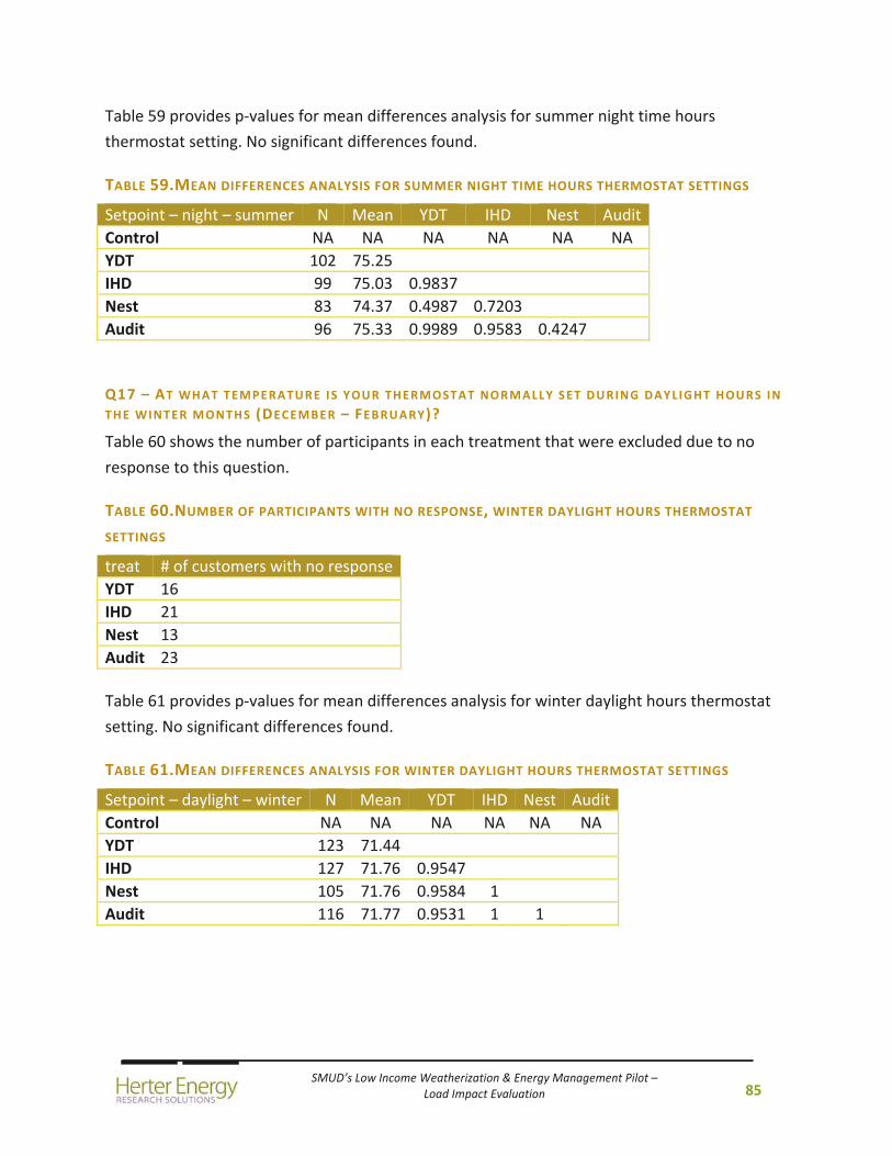
SMUD’s Low Income Weatherization & Energy Management Pilot – Load Impact Evaluation
85
Table 59 provides p‐values for mean differences analysis for summer night time hours
thermostat setting. No significant differences found.
TABLE 59.MEAN DIFFERENCES ANALYSIS FOR SUMMER NIGHT TIME HOURS THERMOSTAT SETTINGS
Setpoint – night – summer N Mean YDT IHD Nest Audit
Control NA NA NA NA NA NA
YDT 102 75.25
IHD 99 75.03 0.9837
Nest 83 74.37 0.4987 0.7203
Audit 96 75.33 0.9989 0.9583 0.4247
Q17 – AT WHAT TEMPERATURE I S YOUR THERMOSTAT NORMALLY SET DURING DAYLIGHT HOURS IN
THE WINTER MONTHS (DECEMBER – FEBRUARY)?
Table 60 shows the number of participants in each treatment that were excluded due to no
response to this question.
TABLE 60.NUMBER OF PARTICIPANTS WITH NO RESPONSE, WINTER DAYLIGHT HOURS THERMOSTAT
SETTINGS
treat # of customers with no response
YDT 16
IHD 21
Nest 13
Audit 23
Table 61 provides p‐values for mean differences analysis for winter daylight hours thermostat
setting. No significant differences found.
TABLE 61.MEAN DIFFERENCES ANALYSIS FOR WINTER DAYLIGHT HOURS THERMOSTAT SETTINGS
Setpoint – daylight – winter N Mean YDT IHD Nest Audit
Control NA NA NA NA NA NA
YDT 123 71.44
IHD 127 71.76 0.9547
Nest 105 71.76 0.9584 1
Audit 116 71.77 0.9531 1 1
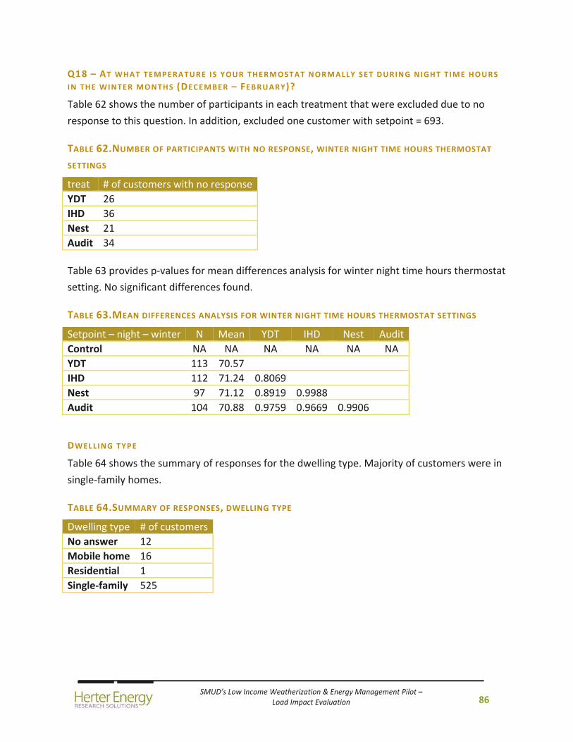
SMUD’s Low Income Weatherization & Energy Management Pilot – Load Impact Evaluation
86
Q18 – AT WHAT TEMPERATURE I S YOUR THERMOSTAT NORMALLY SET DURING NIGHT TIME HOURS
IN THE WINTER MONTHS (DECEMBER – FEBRUARY)?
Table 62 shows the number of participants in each treatment that were excluded due to no
response to this question. In addition, excluded one customer with setpoint = 693.
TABLE 62.NUMBER OF PARTICIPANTS WITH NO RESPONSE, WINTER NIGHT TIME HOURS THERMOSTAT
SETTINGS
treat # of customers with no response
YDT 26
IHD 36
Nest 21
Audit 34
Table 63 provides p‐values for mean differences analysis for winter night time hours thermostat
setting. No significant differences found.
TABLE 63.MEAN DIFFERENCES ANALYSIS FOR WINTER NIGHT TIME HOURS THERMOSTAT SETTINGS
Setpoint – night – winter N Mean YDT IHD Nest Audit
Control NA NA NA NA NA NA
YDT 113 70.57
IHD 112 71.24 0.8069
Nest 97 71.12 0.8919 0.9988
Audit 104 70.88 0.9759 0.9669 0.9906
DWELLING TYPE
Table 64 shows the summary of responses for the dwelling type. Majority of customers were in
single‐family homes.
TABLE 64.SUMMARY OF RESPONSES, DWELLING TYPE
Dwelling type # of customers
No answer 12
Mobile home 16
Residential 1
Single‐family 525
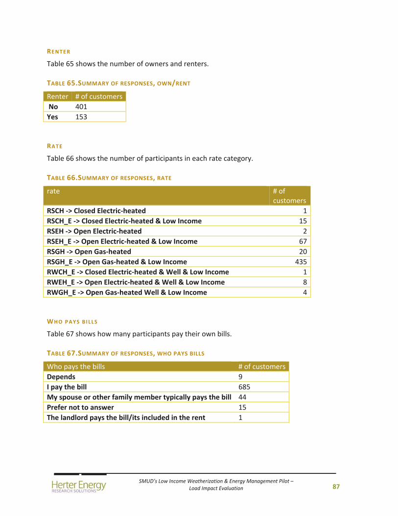
SMUD’s Low Income Weatherization & Energy Management Pilot – Load Impact Evaluation
87
RENTER
Table 65 shows the number of owners and renters.
TABLE 65.SUMMARY OF RESPONSES, OWN/RENT
Renter # of customers
No 401
Yes 153
RATE
Table 66 shows the number of participants in each rate category.
TABLE 66.SUMMARY OF RESPONSES, RATE
rate # of customers
RSCH ‐> Closed Electric‐heated 1 RSCH_E ‐> Closed Electric‐heated & Low Income 15 RSEH ‐> Open Electric‐heated 2 RSEH_E ‐> Open Electric‐heated & Low Income 67 RSGH ‐> Open Gas‐heated 20 RSGH_E ‐> Open Gas‐heated & Low Income 435 RWCH_E ‐> Closed Electric‐heated & Well & Low Income 1 RWEH_E ‐> Open Electric‐heated & Well & Low Income 8 RWGH_E ‐> Open Gas‐heated Well & Low Income 4
WHO PAYS BILLS
Table 67 shows how many participants pay their own bills.
TABLE 67.SUMMARY OF RESPONSES, WHO PAYS BILLS
Who pays the bills # of customers
Depends 9
I pay the bill 685
My spouse or other family member typically pays the bill 44
Prefer not to answer 15
The landlord pays the bill/its included in the rent 1