1

Smoothing Property of Load Variation

Promotes Finding Global Solutions of

Time-Varying Optimal Power FlowJulie Mulvaney-Kemp, Salar Fattahi, and Javad Lavaei

Abstract

This paper analyzes solution trajectories for optimal power flow (OPF) with time-varying load.

Despite its nonlinearity, time-varying OPF is commonly solved every 5-15 minutes using local-search

algorithms. Failing to obtain the globally optimal solution of power optimization problems jeopardizes the

grid’s reliability and causes financial and environmental issues. The objective of this paper is to address

this problem by understanding the optimality behavior of OPF solution trajectories. An empirical study

on California data shows that, with enough variation in the data, local search methods can solve OPF

to global optimality, even if the problem has many local minima. To explain this phenomenon, we

introduce a backward mapping that relates the time-varying OPF’s global solution at a given time to

a set of desirable initial points. We show that this mapping could act as a stochastic gradient ascent

algorithm on an implicitly convexified formulation of OPF, justifying the escape of poor solutions over

time. This work is the first to mathematically explain how temporal data variation affects the complexity

of solving power operational problems.

Index Terms

Optimal power flow, online optimization, global minima, local search

The authors are with the Department of Industrial Engineering and Operations Research, University of California, Berkeley,

Berkeley, CA 94709 USA. e-mail: julie mulvaney-kemp@berkeley.edu; fattahi@berkeley.edu; lavaei@berkeley.edu

A shorter version of this paper has been accepted to the 2020 IEEE Power & Energy Society General Meeting [1]. The new

additions to this version include a case study with 16 feasible trajectories (compared with 4 in the previous version), numerical

analysis highlighting the impact of load variation, an updated model for approximating time-varying OPF, and theoretical analysis

of the problem dynamics over time.

2

I. INTRODUCTION

Optimal power flow (OPF) is a large-scale optimization problem at the core of the daily operation

of power systems world-wide. OPF aims to find a cost-minimizing operating point for a power system,

subject to various operational and security constraints [2]. The OPF problem is challenging because of its

nonconvexity and the frequency at which it is solved [3]. Because demand across the system is constantly

in flux, the OPF problem is solved every few minutes to match the system’s power generation with its

latest demand profile. Nonconvex constraints in the AC model of OPF are the main impediment to solving

the problem efficiently and optimally. Physical laws govern these constraints, indicating nonconvexity is

inherent to the problem. In power systems [4], [5] and in machine learning [6], such nonconvexity

is known to give rise to poor local solutions. To realize the vision of sustainable and resilient power

grids, there is a pressing need to address the nonconvexity and timescale of both existing and emerging

optimization problems for the control and operation of the grid. Since these problems are all built upon

the power flow equations, we focus on OPF in this paper.

With the goal of addressing the underlying nonconvexity of the problem, a recent line of research

has focused on approximating the problem as a single or sequence of convex optimization problems.

These works include quadratic convex [7], second-order conic programming [8], and semidefinite pro-

gramming [9]–[11] relaxations. Despite desirable theoretical guarantees, the convex relaxations of OPF

suffer from two major drawbacks: 1) Their global guarantees often come at the expense of higher runtimes

or overly complicated implementations; 2) They do not account for the time-varying nature of demand.

This time-varying property poses additional constraints on the ramping capabilities of generators, which

in turn gives rise to coupled optimization problems.

On the other hand, research on multiperiod OPF, such as [12], [13], and dyanamic OPF, such

as [14], [15], endeavors to solve multiple such time-coupled OPF problems simultaneously. This leads to

large problem formulations which are still nonconvex in nature. As a result, solution strategies for these

problems often rely on the convex relaxations discussed previously in combination with receding horizon

approaches or nonlinear programming algorithms, which lack global optimality guarantees [12]. Another

drawback is that the data for all time periods must be specified at the outset. In practice, forecasts may

not be adequately accurate far in advance.

Real-time OPF is another approach which targets the timescale of OPF. In [16] a real-time

algorithm is used to track the optimal solution every few seconds in between traditional OPF updates,

which occur on a slower timescale ranging from every 5 to 30 minutes. It uses new measurements of the

decision variables’ values and constraints at every time step in order to compute a correction and track

3

the optimal solution. The correction is computed by solving a quadratic optimization problem with one

iteration of a quasi-Newton algorithm. This has the advantage of responding quickly to fluctuations, but

does not replace the need to solve OPF on the traditional timescale. Other faster-timescale approaches

to OPF-related problems include [17]–[19].

In this work, which is positioned between MPOPF and real-time OPF, we consider time-varying

OPF with ramping constraints in an online fashion, where the load profile changes over time. Unlike

the previous convexification techniques, we solve the problem sequentially using a simple local-search

algorithm. Due to the nonconvex nature of the problem, the local-search algorithm may return a spurious

(non-global) local solution, thus leading to a potentially large optimality gap. Previously in [20], we

made the observation that for a small system with time-varying demand, the solution trajectories of the

time-varying OPF stemming from four initial local solutions could converge over time. Here, we present

an extensive empirical study on a larger system with 16 spurious solutions using California load data, and

show that all feasible local solution sequences (also called trajectories) converge in cost and value to the

best solution. Notably, this phenomenon occurs despite the fact that the problem has multiple point-wise

poor local minima at key times. For this system, we show that there is an escaping period in which

different local solution trajectories converge to a solution with lowest cost, followed by a tracking period

in which the local trajectories closely track the global solution.

This observation leads to an important phenomenon in time-varying OPF: load variation enables

the local solution trajectories to avoid poor solutions over time.1 In other words, despite the highly

nonconvex nature of the OPF problem at any given time, our numerical algorithm acts on an implicitly

smoothed and well-behaved variant of the problem, thereby avoiding the undesirable local solutions over

time. We will formalize this statement in the paper by providing a backward-in-time mapping from the

globally optimal solutions of OPF at a given time (namely, end of the escaping period) to the set of

desirable initial points. By leveraging its special structure, we show that the proposed backward mapping

may act as a stochastic gradient ascent algorithm on an implicitly convexified formulation of the OPF

problem, which in turn explains why local solution trajectories could avoid poor solutions over time. This

work is the first studying the role of data variation in reducing the complexity of power optimization

problems. Since it relies on simple local search methods, the solution techniques have extremely low

memory and time complexities and can also be implemented in a distributed setting to accommodate the

distributed nature of future grids [21].

1Note that with constant (time-invariant) load, all the local solution trajectories will remain unchanged over time.

4

II. EMPIRICAL STUDY OF TIME-VARYING OPF

In this section, we analyze the local solution trajectories of time-varying OPF primarily for

a 39-bus system. A secondary analysis on a 9-bus system is also shared to highlight that the observed

behavior is not unique to the 39-bus system. The solution trajectories of time-varying OPF are constructed

by sequentially solving a series of optimization problems with time-varying demand levels using a local-

search algorithm. California load data and synthetic load scenarios are used to determine demand levels

over time. To prevent the solution from changing abruptly over a short period of time, the sequential

optimization problems are coupled via so-called ramping constraints, as we explain below.

A. Model and Algorithm Details

To examine the behavior of different local solution trajectories, we consider a modified version

of the IEEE 39-bus system, as introduced in [4]. Specifically, the real and reactive power demands are

reduced by 50%, voltage limits tightened from +/-6% to +/-5%, and the cost functions associated with all

generators are assumed to be linear. The OPF problem for this system with a generation cost-minimizing

objective and fixed demand values is known to have 16 local solutions. In this work, we take into account

the time-varying nature of the load and scale all demands proportionally to a given load profile. Finally,

we introduce the ramping constraints that limit the change in power generation for each generator over

time.

Starting from the 16 known initial local solutions, we constructed the sequences of local trajecto-

ries using the MATPOWER optimization toolbox [22] and fmincon sequential quadratic programming

solver2 in the following procedure. We ran Algorithm 1 for all 16 initial local solutions and obtained 16

different solution sequences, which are called discrete local trajectories [20].

2Note that unlike many interior point methods that require strictly feasible initial points, fmincon sequential quadratic

programming gives a second-order critical point even if the initial point is not strictly feasible.

0 5 10 15 20 25

Time (hours after 3:00 a.m.)

1

1.2

1.4

1.6

Dem

and s

calin

g facto

r

Fig. 1: Average daily net load for California during August 2019 [23]

5

Algorithm 1 Algorithm for obtaining discrete local trajectoriesInput: Power system model with a fixed initial point x0, demand curve, ramping constraint specifications

Output: Discrete local trajectory {xt}Kt=0

1: Initialization : t = 1

2: for every 15-minute time increment over 24 hours do

3: Set demand constraints for each bus according to the demand curve at time t.

4: Set generator production limits based on xt−1 and the ramping constraint.

5: Solve the resulting cost-minimization OPF problem with fixed demand and initial point xt−1 using

fmincon. Upon feasibility, collect the solution as xt.

6: end for

7: return {xt}Tt=0

B. Behavior of Discrete Local Trajectories for a 39-bus system with California Data

In this example, the shape of the demand curve is based on the California’s net load for an average

day in August 2019 [23] (Fig. 1). The reported actual hourly net load data was interpolated linearly to

produce a net load estimate for each 15-minute interval within 24 hours. The curve is normalized and

shifted so that time 0 represents 3:00 a.m. Here, the maximum magnitude of allowable change in power

generation between two consecutive time steps is 10% of the capacity of each generator. All 16 discrete

local trajectories remain feasible throughout the span of twenty-four hours. (This is not guaranteed, as

local search may not always find a feasible point or such point may not even exist.) Fig. 2 shows the

point-wise distance between these feasible trajectories and the feasible trajectory with the lowest cost

(labeled as Trajectory 2). Interestingly, all 16 trajectories converge to Trajectory 2 within nine hours.

0 5 10 15 20 25

Time (hours after 3:00 a.m.)

0

500

1000

1500

Dis

tan

ce

to

be

st

tra

jecto

ry s

olu

tio

n

Trajectory1

Trajectory2

Trajectory3

Trajectory4

Trajectory5

Trajectory6

Trajectory7

Trajectory8

Trajectory9

Trajectory10

Trajectory11

Trajectory12

Trajectory13

Trajectory14

Trajectory15

Trajectory16

Fig. 2: Solution convergence for points on discrete local trajectories

6

Based on this observation, one may speculate that the problem becomes devoid of spurious

local solutions over time. This is not the case for the considered problem. We uniformly searched the

feasible region of the problem without ramping constraints and verified that there are multiple point-

wise spurious local solutions for the point-wise (single time instance, without ramping constraints) OPF

problem at different times. In particular, there are many local solutions around the escape time (hour

9) when the discrete local trajectories merge into one trajectory. Fig. 3 shows the normalized objective

cost values for different discrete local trajectories, alongside the costs of the discovered point-wise local

solutions. Despite the existence of multiple sub-optimal operating points at different times, the discrete

local trajectories initialized at various local solutions result in the lowest cost values over time. Fig. 4

examines the active and reactive power generation for two representative generators. This figure shows

that the problem has point-wise local solutions with a wide range of generation levels, highlighting the

importance of finding the solution with the lowest cost.

Observe that most of the spurious point-wise local solutions have sharp and random nature. In

other words, they appear at different time-steps with various cost values, and then quickly disappear after

a short period of time. This implies that the landscape of OPF may be highly nonconvex at any given

time step. However, it can be observed that our numerical algorithm is not affected by such sharp local

solutions. To explain this phenomena, we will show in Section IV that the data variation enables the

solver to act on a smoothed version of the problem that is devoid of sharp local minima.

0 5 10 15 20 25

Time (hours after 3:00 a.m.)

0

1

2

3

4

5

6

Obje

ctive c

ost -

low

est tr

aje

cto

ry c

ost

Point-wise local solution

Fig. 3: Cost for points on discrete local trajectories and point-wise local solutions (for a single instance of OPF), relative to the cost of the best

trajectory

C. Behavior of Discrete Local Trajectories for a 9-bus system with California Data

In this example, we consider a modified version of the IEEE 9-bus system with 4 known local

solutions to the OPF problem, as introduced in [4]. Specifically, the active and reactive power demands

7

0 5 10 15 200

200

400

600

Real pow

er

Bus 31

0 5 10 15 20

Time (hours after 3:00 a.m.)

0

100

200

Reactive p

ow

er

0 5 10 15 200

200

400

600

Real pow

er

Bus 35

0 5 10 15 20

Time (hours after 3:00 a.m.)

-100

0

100

Reactive p

ow

er

Fig. 4: Real and reactive power output of select generators: points on discrete local trajectories and point-wise local solutions

1200 1600 2000 2400 0400 0800 1200

Time of day

1

1.5

2

De

ma

nd

sca

ling

fa

cto

r

(a) Average daily net load for California during May 2019 [23]

1200 1600 2000 2400 0400 0800 1200

Time of day

0

500

1000

Obje

ctive c

ost -

low

est tr

aje

cto

ry c

ost Trajectory 1

Trajectory 2

Trajectory 3

Trajectory 4

Point-wise local solution

(b) Cost for points on discrete local trajectories and point-wise local solutions (for a single instance of OPF), relative to the cost of the best trajectory

Fig. 5: Data and results for an empirical study on a 9-bus system

are reduced by 40% and the lower bounds on reactive power compensation are tightened to -5 Mvar.

The demand data is a normalized and shifted version of California’s net load for an average day in May

2019 [23] (Fig. 5a). Fig. 5b shows the relative objective cost values for different discrete local trajectories,

alongside the costs of the discovered point-wise local solutions, produced using Algorithm 1 with a 5%

ramping constraint. Again, we observe that the load variation enables all trajectories to converge to the

optimal trajectory.

8

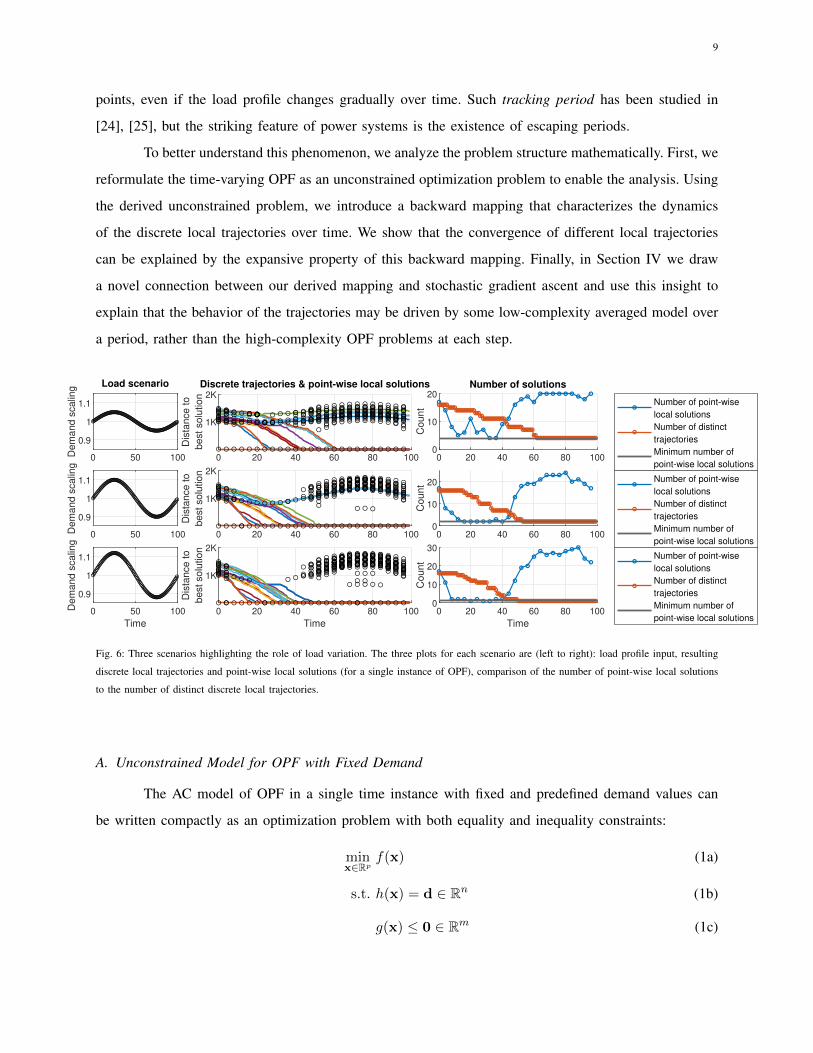
D. Impact of Load Variation on 39-bus System

Next, we consider discrete local trajectories for three different load profiles on the same 39-bus

system. Isolating the impact of load variation enables insight into how variation creates trajectories that

avoid poor solutions, as occurred in the previous examples. The three demand curves used are sinusoidal

functions with amplitudes representing 5%, 10% and 12% deviation from the initial load, as shown in the

left column of Fig. 6. The ramping constraint (i.e., maximum magnitude of allowable change in power

generation between two consecutive time steps) is 5% of the capacity of each generator. In each scenario,

all 16 discrete local trajectories remain feasible throughout the time horizon (100 steps).

The results show that larger magnitudes of data variation lead to fewer poor solutions over time.

At 5% variation 4 trajectories remain at 4 different poor solutions, while the remaining 12 trajectories

converge to the best solution. At 10% variation 3 trajectories converge to the same poor solution, while the

remaining 13 trajectories converge to the best solution. At 12% variation all 16 trajectories converge to the

best known solution. These results are displayed in the center column of Fig. 6, which shows the distance

between each trajectory and the trajectory with the lowest cost, along with discovered point-wise local

solutions. The search for point-wise local solutions is done every fourth time step due to the significant

computational effort required to repeatedly solve the problem from a range of initial points. Fig. 6 (right

column) compares the number of point-wise local solutions with the number of distinct3 trajectories over

time. In these three cases, the number of distinct trajectories decreases until it plateaus at the minimum

number of point-wise local solutions found over the entire period. This offers one potential explanation of

how load variation creates trajectories that escape poor solutions: In exploring a range of static problems,

you may encounter one or more times at which the problem has a favorable landscape4. At such times,

the coupled problem may escape a poor solution. Eventually, the number of poor trajectories is limited

by the number of spurious point-wise local solutions of the most favorable landscape.

III. MATHEMATICAL ANALYSIS OF TIME-VARYING OPF

The case study in Section II reveals an important property of the time-varying OPF problem: In

the escaping period, different discrete local trajectories converge to the operating point with the lowest

cost. Then, in the tracking period, the discrete local trajectories track these globally optimal operating

3Solutions are considered distinct if the real or reactive power output at any generator differs by at least 1 MW or 1 MVAr,

respectively, or if the voltage magnitude or angle at any bus differs by at least 10−3 p.u. (345V) or 10−3 radians, respectively.4The number of spurious point-wise local solutions is an indicator of how difficult a given static OPF problem is. If only one

point-wise local solution is found, the problem may be convex. However, the search is not exhaustive, so other local minima

with small regions of attraction may exist.

9

points, even if the load profile changes gradually over time. Such tracking period has been studied in

[24], [25], but the striking feature of power systems is the existence of escaping periods.

To better understand this phenomenon, we analyze the problem structure mathematically. First, we

reformulate the time-varying OPF as an unconstrained optimization problem to enable the analysis. Using

the derived unconstrained problem, we introduce a backward mapping that characterizes the dynamics

of the discrete local trajectories over time. We show that the convergence of different local trajectories

can be explained by the expansive property of this backward mapping. Finally, in Section IV we draw

a novel connection between our derived mapping and stochastic gradient ascent and use this insight to

explain that the behavior of the trajectories may be driven by some low-complexity averaged model over

a period, rather than the high-complexity OPF problems at each step.

0 50 100

0.9

1

1.1

Dem

and s

calin

g Load scenario

0 20 40 60 80 100

1K

2K

Dis

tance to

best solu

tion

Discrete trajectories & point-wise local solutions

0 20 40 60 80 1000

10

20

Count

Number of solutions

Number of point-wise

local solutions

Number of distinct

trajectories

Minimum number of

point-wise local solutions

0 50 100

0.9

1

1.1

Dem

and s

calin

g

0 20 40 60 80 100

1K

2K

Dis

tance to

best solu

tion

0 20 40 60 80 1000

10

20

Count

Number of point-wise

local solutions

Number of distinct

trajectories

Minimum number of

point-wise local solutions

0 50 100

Time

0.9

1

1.1

Dem

and s

calin

g

0 20 40 60 80 100

Time

1K

2K

Dis

tance to

best solu

tion

0 20 40 60 80 100

Time

0

10

20

30

Count

Number of point-wise

local solutions

Number of distinct

trajectories

Minimum number of

point-wise local solutions

Fig. 6: Three scenarios highlighting the role of load variation. The three plots for each scenario are (left to right): load profile input, resulting

discrete local trajectories and point-wise local solutions (for a single instance of OPF), comparison of the number of point-wise local solutions

to the number of distinct discrete local trajectories.

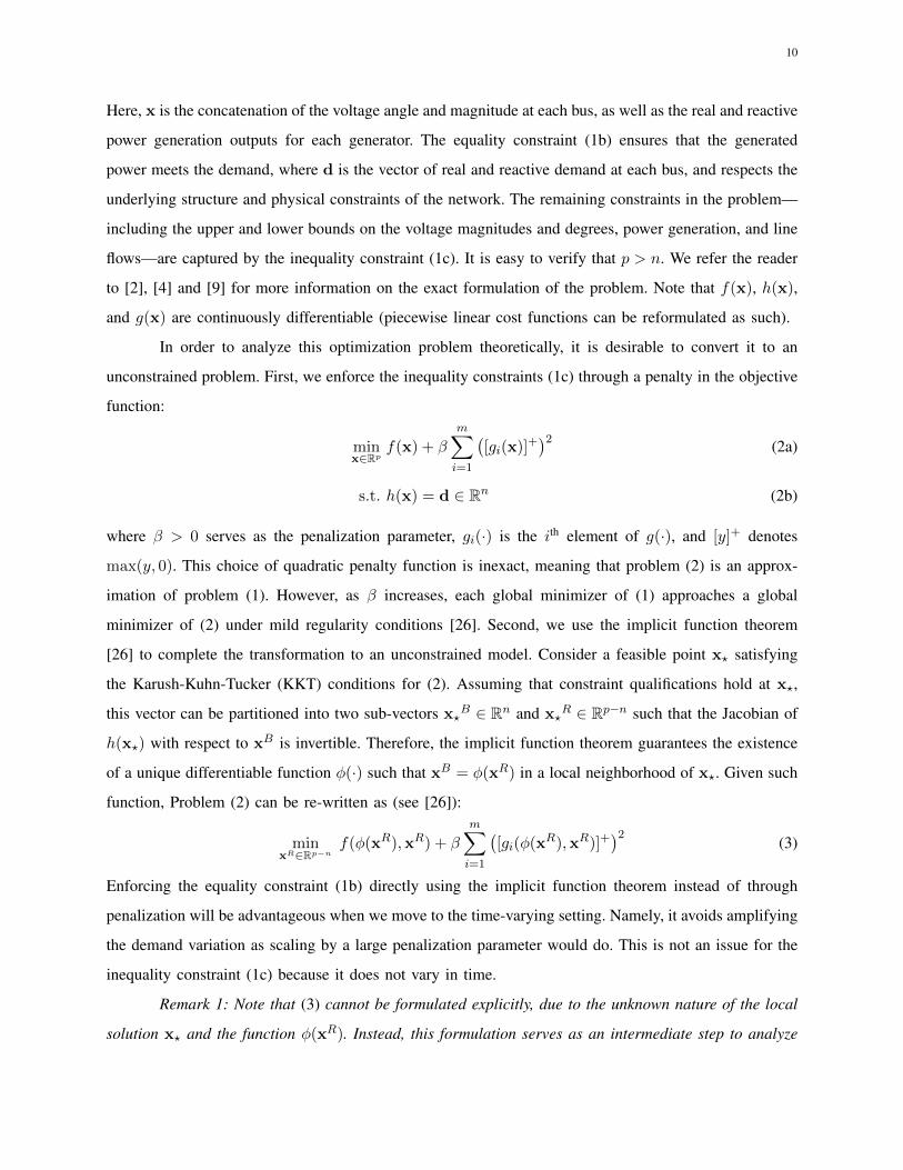
A. Unconstrained Model for OPF with Fixed Demand

The AC model of OPF in a single time instance with fixed and predefined demand values can

be written compactly as an optimization problem with both equality and inequality constraints:

minx∈Rp

f(x) (1a)

s.t. h(x) = d ∈ Rn (1b)

g(x) ≤ 0 ∈ Rm (1c)

10

Here, x is the concatenation of the voltage angle and magnitude at each bus, as well as the real and reactive

power generation outputs for each generator. The equality constraint (1b) ensures that the generated

power meets the demand, where d is the vector of real and reactive demand at each bus, and respects the

underlying structure and physical constraints of the network. The remaining constraints in the problem—

including the upper and lower bounds on the voltage magnitudes and degrees, power generation, and line

flows—are captured by the inequality constraint (1c). It is easy to verify that p > n. We refer the reader

to [2], [4] and [9] for more information on the exact formulation of the problem. Note that f(x), h(x),

and g(x) are continuously differentiable (piecewise linear cost functions can be reformulated as such).

In order to analyze this optimization problem theoretically, it is desirable to convert it to an

unconstrained problem. First, we enforce the inequality constraints (1c) through a penalty in the objective

function:

minx∈Rp

f(x) + β

m∑i=1

([gi(x)]+

)2 (2a)

s.t. h(x) = d ∈ Rn (2b)

where β > 0 serves as the penalization parameter, gi(·) is the ith element of g(·), and [y]+ denotes

max(y, 0). This choice of quadratic penalty function is inexact, meaning that problem (2) is an approx-

imation of problem (1). However, as β increases, each global minimizer of (1) approaches a global

minimizer of (2) under mild regularity conditions [26]. Second, we use the implicit function theorem

[26] to complete the transformation to an unconstrained model. Consider a feasible point x? satisfying

the Karush-Kuhn-Tucker (KKT) conditions for (2). Assuming that constraint qualifications hold at x?,

this vector can be partitioned into two sub-vectors x?B ∈ Rn and x?

R ∈ Rp−n such that the Jacobian of

h(x?) with respect to xB is invertible. Therefore, the implicit function theorem guarantees the existence

of a unique differentiable function φ(·) such that xB = φ(xR) in a local neighborhood of x?. Given such

function, Problem (2) can be re-written as (see [26]):

minxR∈Rp−n

f(φ(xR),xR) + β

m∑i=1

([gi(φ(xR),xR)]+

)2(3)

Enforcing the equality constraint (1b) directly using the implicit function theorem instead of through

penalization will be advantageous when we move to the time-varying setting. Namely, it avoids amplifying

the demand variation as scaling by a large penalization parameter would do. This is not an issue for the

inequality constraint (1c) because it does not vary in time.

Remark 1: Note that (3) cannot be formulated explicitly, due to the unknown nature of the local

solution x? and the function φ(xR). Instead, this formulation serves as an intermediate step to analyze

11

the behavior of discrete local trajectories over time. In other words, one would solve the OPF problem

directly in practice, and the surrogate problem (3) is designed to understand the properties of OPF.

B. Unconstrained Model for Time-Varying OPF

The above analysis reveals that, under some technical conditions, the OPF problem with fixed

load can be modeled as an unconstrained optimization problem (with a controllable approximation error).

In this subsection, we extend our analysis to time-varying OPF where demand changes over time and

the problem must respect ramping constraints. As previously stated, ramping constraints ensure that the

solution does not change too drastically from one time step to the next. One way to softly impose ramping

constraints is through a proximal method, which penalizes the distance between the current and previous

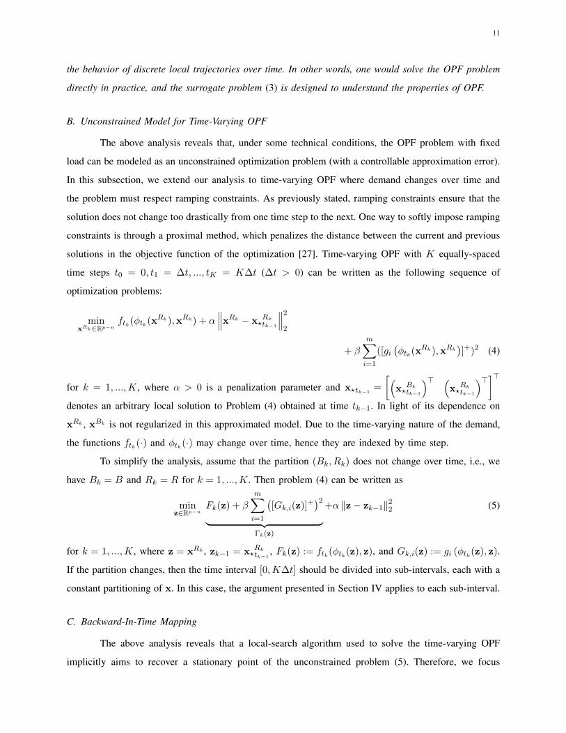
solutions in the objective function of the optimization [27]. Time-varying OPF with K equally-spaced

time steps t0 = 0, t1 = ∆t, ..., tK = K∆t (∆t > 0) can be written as the following sequence of

optimization problems:

minxRk∈Rp−n

ftk(φtk(xRk),xRk) + α

∥∥∥xRk − x?Rktk−1

∥∥∥2

2

+ β

m∑i=1

([gi(φtk(x

Rk),xRk)]+)2 (4)

for k = 1, ...,K, where α > 0 is a penalization parameter and x?tk−1=

[(x?

Bktk−1

)> (x?

Rktk−1

)>]>denotes an arbitrary local solution to Problem (4) obtained at time tk−1. In light of its dependence on

xRk , xBk is not regularized in this approximated model. Due to the time-varying nature of the demand,

the functions ftk(·) and φtk(·) may change over time, hence they are indexed by time step.

To simplify the analysis, assume that the partition (Bk, Rk) does not change over time, i.e., we

have Bk = B and Rk = R for k = 1, ...,K. Then problem (4) can be written as

minz∈Rp−n

Fk(z) + β

m∑i=1

([Gk,i(z)]+

)2︸ ︷︷ ︸

Γk(z)

+α ‖z− zk−1‖22 (5)

for k = 1, ...,K, where z = xRk , zk−1 = x?Rktk−1

, Fk(z) := ftk(φtk(z), z), and Gk,i(z) := gi (φtk(z), z).

If the partition changes, then the time interval [0,K∆t] should be divided into sub-intervals, each with a

constant partitioning of x. In this case, the argument presented in Section IV applies to each sub-interval.

C. Backward-In-Time Mapping

The above analysis reveals that a local-search algorithm used to solve the time-varying OPF

implicitly aims to recover a stationary point of the unconstrained problem (5). Therefore, we focus

12

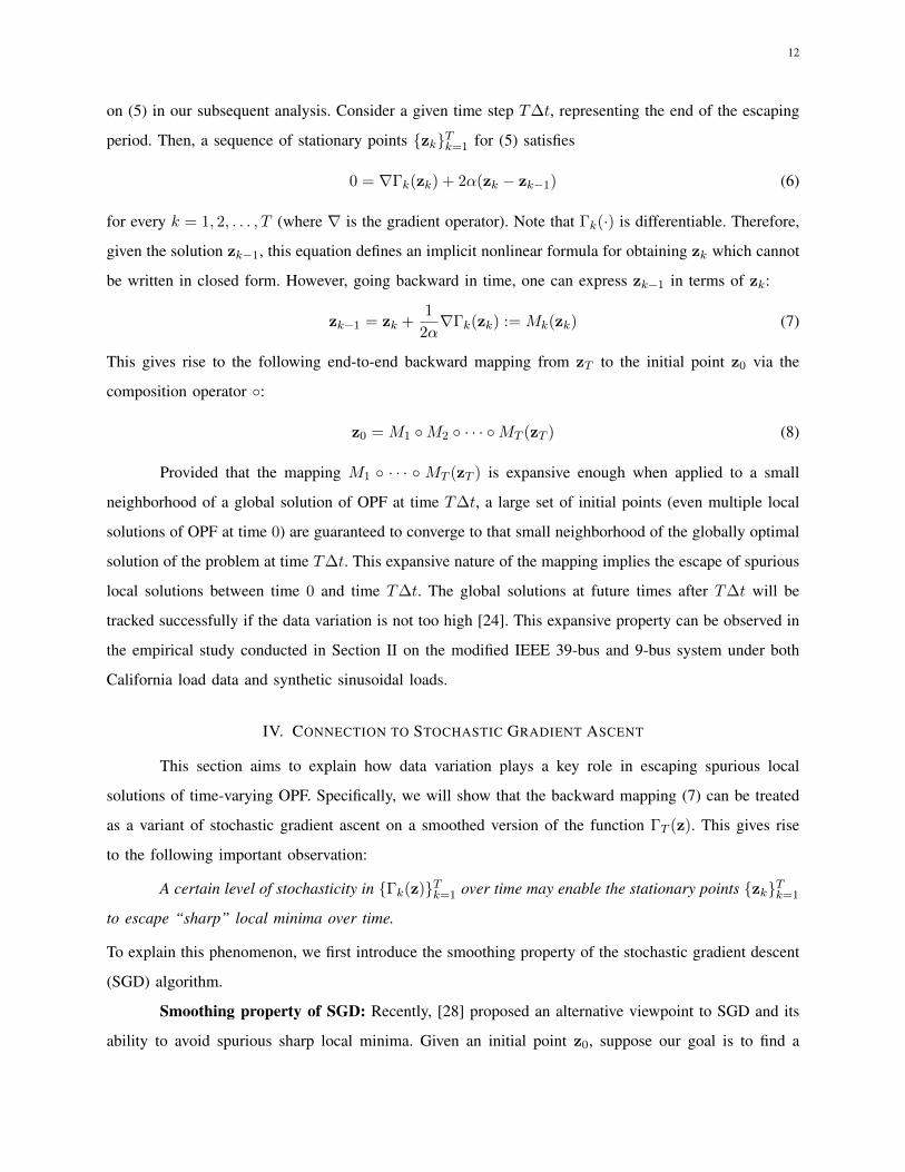
on (5) in our subsequent analysis. Consider a given time step T∆t, representing the end of the escaping

period. Then, a sequence of stationary points {zk}Tk=1 for (5) satisfies

0 = ∇Γk(zk) + 2α(zk − zk−1) (6)

for every k = 1, 2, . . . , T (where ∇ is the gradient operator). Note that Γk(·) is differentiable. Therefore,

given the solution zk−1, this equation defines an implicit nonlinear formula for obtaining zk which cannot

be written in closed form. However, going backward in time, one can express zk−1 in terms of zk:

zk−1 = zk +1

2α∇Γk(zk) := Mk(zk) (7)

This gives rise to the following end-to-end backward mapping from zT to the initial point z0 via the

composition operator ◦:

z0 = M1 ◦M2 ◦ · · · ◦MT (zT ) (8)

Provided that the mapping M1 ◦ · · · ◦ MT (zT ) is expansive enough when applied to a small

neighborhood of a global solution of OPF at time T∆t, a large set of initial points (even multiple local

solutions of OPF at time 0) are guaranteed to converge to that small neighborhood of the globally optimal

solution of the problem at time T∆t. This expansive nature of the mapping implies the escape of spurious

local solutions between time 0 and time T∆t. The global solutions at future times after T∆t will be

tracked successfully if the data variation is not too high [24]. This expansive property can be observed in

the empirical study conducted in Section II on the modified IEEE 39-bus and 9-bus system under both

California load data and synthetic sinusoidal loads.

IV. CONNECTION TO STOCHASTIC GRADIENT ASCENT

This section aims to explain how data variation plays a key role in escaping spurious local

solutions of time-varying OPF. Specifically, we will show that the backward mapping (7) can be treated

as a variant of stochastic gradient ascent on a smoothed version of the function ΓT (z). This gives rise

to the following important observation:

A certain level of stochasticity in {Γk(z)}Tk=1 over time may enable the stationary points {zk}Tk=1

to escape “sharp” local minima over time.

To explain this phenomenon, we first introduce the smoothing property of the stochastic gradient descent

(SGD) algorithm.

Smoothing property of SGD: Recently, [28] proposed an alternative viewpoint to SGD and its

ability to avoid spurious sharp local minima. Given an initial point z0, suppose our goal is to find a

13

global minimum of a (time-invariant) function Γ(z) using SGD. Accordingly, the iterations of SGD can

be written

zk+1 = zk − η(∇Γ(zk) + ωk) ∀k ∈ {0, 1, 2, . . . } (9)

where ωt is a bounded random variable with zero mean and η is a predefined step size. Upon defining

zk = zk − η∇Γ(zk), one can write the above iterations (9) in terms of the intermediate sequence {zk}:

zk+1 = zk−ηωk−η∇Γ(zk−ηωk),∀k ∈ {0, 1, 2, . . . } (10)

To analyze the average behavior of SGD, consider the evolution of Eωk(zk+1), where the expectation is

taken over ωk conditioned on {ω0, . . . , ωk−1}. Hence,

Eωk [zk+1]= zk−η∇Eωk [Γ(zk−ηωk)],∀k∈{0,1,2,. . .} (11)

Therefore, on average, SGD acts as the exact gradient descent on the surrogate function Eωk [Γ(zk − ηωk)].

Comparing this function with Γ(z), one can verify that the former is a smoothed version of the latter, where

the smoothness is due to the convolution of Γ(z) with the probability density function of the random

variable ωk. As illustrated in [28], such convolution may give rise to (one-point) strong convexity of

Eωk [Γ(zk − ηωk)] with respect to the globally optimal solution, which in turn guarantees the convergence

of {zk} (and hence {zk}) to a small neighborhood around the global solution, even in the presence of

sharp local minima. A key takeaway from this observation is that Γ(z) can possess multiple sharp, poor

local minima, and yet its smoothed version Eωk [Γ(zk − ηωk)] may be devoid of such solutions.

Time-varying optimization and time-varying OPF: Returning to time-varying OPF and the

backward mapping (7), we assume that the variation in {∇Γk(z)}Tk=1 follows a stochastic process indexed

by the time k. In particular, we write ∇Γk(z)−∇Γk+1(z) = ζk(z) +ωk, where ζk(z) is a deterministic,

time-varying function and ωk is a bounded random variable with zero mean. Such assumption is realistic

in power systems, where demand can be modeled as a deterministic, time-varying function capturing the

average demand behavior, together with an additive stochastic term accounting for its random nature.

The iteration (7) is equivalent to

zk =zk+1 +1

2α∇ΓT (zk+1)

+1

2α

T−1∑τ=k+1

(∇Γτ (zk+1)−∇Γτ+1(zk+1))︸ ︷︷ ︸ζτ (zk+1)−ωτ

(12)

which can be written as the following dynamical model:

zk = zk+1 +1

2α∇ΓT (zk+1) +

1

2ανk+1(zk+1) (13a)

νk+1(zk+1) = νk+2(zk+1) + ζk+1(zk+1)− ωk+1 (13b)

14

where νk+1(zk+1) is referred to as the variation process. In particular, (13b) defines explicit dynamics for

the variation process comprised of three parts. The first term νk+2(zk+1) captures the correlation between

the variation processes at times tk+1 and tk+2. The second term ζk+1(zk+1) captures the bias that is

added to the variation process at time tk+1. Lastly, the third term ωk+1 ∼ W (zk+1) is an independent

noise injected into the variation process at time tk+1 (also referred to as effective noise). Comparing (13)

with (9), one can verify that (13) reduces to stochastic gradient ascent if νk+2(zk+1) + ζk+1(zk+1) = 0.

Therefore, if ωk+1 dominates the first two terms, (13) resembles an approximate version of stochastic

gradient ascent applied to ΓT (z); otherwise, it is a biased and correlated version of SGD [29]. Similar

to (11), this implies that, on average, the points generated via the backward mapping (7) would be close

to the iterations of the gradient ascent on the smoothed version of ΓT (z). Now, assume that despite the

possible existence of multiple spurious and sharp local minima in {Γk(z)}Tk=1, the smoothed version of

ΓT (z) after convolution is strongly convex. This together with the expansive nature of gradient ascent

on strongly convex functions [30] yields that the end-to-end backward mapping (8) is expansive, and the

discrete local trajectories can escape poor local solutions over time. We formalize and rigorously analyze

this intuition in the next subsection.

A. Theoretical analysis of dynamics

For simplicity of notation, we define η = 12α . Furthermore, suppose that z∗ denotes the globally

minimum point of ΓT (z). Without loss of generality, ‖v‖ is used to refer to the 2-norm of the vector v.

We make the following assumptions for the dynamical model (13):

Assumption 1 (Smoothness): The following statements hold:

- The function ΓT (z) is L-smooth, i.e., we have

‖∇ΓT (x)−∇ΓT (y)‖ ≤ L‖x− y‖ ∀x,y ∈ Rp−n. (14)

- The functions ζτ (z) are l-Lipschitz for τ = 1, · · · , T − 1, i.e., we have

‖ζk(x)− ζk(y)‖ ≤ l‖x− y‖ ∀x,y ∈ Rp−n. (15)

Assumption 2 (Implicit Convexity): There exists z∗ such that the following statements hold:

- (One-point strong convexity of convolution) For every y, there exists c > 0 such that

〈z∗ − y,−∇Eω∼W (z) [ΓT (y − ηω)]〉 ≥ c‖y − z∗‖2 (16)

- (Bounded one-point curvature of convolution) For every y, there exists c′ > 0 such that

〈z∗−y,−T−1∑τ=k+1

Eω∼W (z) [ζτ (y−ηω)]〉≥−c′‖y − z∗‖2 (17)

15

for every k ∈ {0, . . . , T − 2}.

The existence of L and l which satisfy Assumption 1 can be verified for the unconstrained model of the

time-varying OPF. Meanwhile, Assumption 2 implies that the convoluted variant of the objective function

at time T is one-point strongly convex. We note that such assumption may not be easily verifiable for

the time-varying OPF. However, our simulations strongly support the fact that most of the spurious local

solutions in time-varying OPF have a sharp nature, and therefore, they are likely to be absent in the

convoluted (smoothed) landscape of the problem.

Under these two assumptions, we present the main theorem of this paper.

Theorem 1: Suppose that c ≥ c′ and there exists r ≥ 1 such that ‖ωt‖ ≤ r for every t. Define

λ := η(c − c′), and assume that 2η2L < 1. Then, under Assumptions 1 and 2, the following inequality

holds:

‖zT−z∗‖2≤1

1−2η2L

D+E[‖z0 − z∗‖2

](1 + λ)T−1

+8η2r2T 2

(1 + λ)T−1

(18)

where

D =

(4

λ+

4

λ2

)η3r2l + 16

(1 +

1

λ

)2 η2r2(1 + 2λ)2

λ2(19)

A sketch of the proof for Theorem 1 is provided in the appendix. A number of observations can be

made based on this theorem. Not surprisingly, the provided bound on ‖zT−z∗‖ depends on the accuracy

of the initial point ‖z0 − z∗‖. However, the effect of this initial accuracy diminishes exponentially fast

with respect to T . Moreover, as T →∞, the following asymptotic inequality holds:

‖zT−z∗‖2 ≤D

1− 2η2L(20)

which is independent of the initial point. Another implication of this asymptotic bound is that, for any

value of T , Theorem 1 can only guarantee the convergence of zT to a neighborhood of z∗. This is not

surprising if we consider the non-diminishing nature of η and its connection to SGD, as delineated in the

introduction of Section IV. Indeed, similar results on SGD show that, with non-diminishing step-sizes,

the iterations of the algorithm may only converge to a neighborhood of the globally optimal solution [28].

Finally, it is worthwhile to study how D depends on different parameters of problem, namely η, r, l, L, and

c−c′. Equation (19) reveals that D is a decreasing function of c−c′. Combined with Assumption 2, this

implies that one-point strong convexity of Γt(z) for t = 1, . . . , T has a favorable effect on ‖zT−z∗‖.

Similarly, it can be seen from (18) and (19) that ‖zT−z∗‖ decreases as l, L, and the noise values’

magnitude (characterized by r) shrink. However, notice that Assumption 2 may not be satisfied for small

values of noise. Finally, D does not have a monotone behavior with respect to η. In particular, it can

16

Fig. 7: The 2-bus system. Here, i =√−1.

be verified that D → ∞ if η → ∞ or η → 0+. Recalling (5) and η = 12α , this implies that over- or

under-regularization may lead to large values for ‖zT−z∗‖. This observation is in line with Example 1

of [20], which shows that both small and large regularization may cause the solution trajectory to remain

trapped at spurious local solutions of a time-varying optimization.

B. Illustrative Example on a 2-bus System

In this subsection, we analyze the effect of the load variation on the landscape of a 2-bus system.

Our goal is to visualize the smoothing effect of the load variation on the objective function, thereby

verifying the assumption on the implicit one-point strong convexity of the convoluted objective function.

Consider the simple 2-bus system illustrated in Figure 7. Assume that both buses are equipped with

generators, and they are connected via a single line with admittance g − ib. The time-varying load

connected to the first bus has both active and reactive power demands, while the time-varying load

connected to the second bus is purely active. At any given time k, the point-wise OPF (without ramping

17

constraints) can be formulated as follows5:

min f1(P g1 ) + f2(P g2 ) (21a)

s.t. P g1 −Pl1;k= |v1|2g+|v1||v2|b sin(∆θ)−|v1||v2|g cos(∆θ) (21b)

P g2 −Pl2;k= |v2|2g+|v1||v2|b sin(∆θ)−|v1||v2|g cos(∆θ) (21c)

Qg1−Ql1;k= |v1|2g−|v1||v2|g sin(∆θ)−|v1||v2|b cos(∆θ) (21d)

Qg2 = |v2|2g−|v1||v2|g sin(∆θ)−|v1||v2|b cos(∆θ) (21e)

V min ≤ |v1| ≤ V max, V min ≤ |v2| ≤ V max (21f)

Pmin1 ≤ P g1 ≤ P

max1 , Pmin

2 ≤ P g2 ≤ Pmax2 (21g)

Qmin1 ≤ Qg1 ≤ Q

max1 , Qmin

2 ≤ Qg2 ≤ Qmax2 (21h)

where P gi , Qgi , |vi|, ∆θ are the variables for active power generation, reactive power generation, voltage

magnitude at bus i, and angle difference between buses 1 and 2 respectively. Moreover, P li;k, Qli;k are the

active and reactive load parameters at bus i and time k, respectively. To simplify our subsequent analysis,

we assume that the voltage magnitudes at both buses are equal to the their nominal values, i.e., |v1| =

|v2| = 1. Therefore, according to (21b)-(21e), the variables (P g1 , Pg2 , Q

g1, Q

g2) can be written in terms of

the angle differences ∆θ. In other words, P g1 = p1(∆θ, P l1;k), P g2 = p2(∆θ, P l2;k), Qg1 = q1(∆θ,Ql1;k),

Qg2 = q2(∆θ) where

p1(∆θ, P l1;k) = P l1;k + g + b sin(∆θ)− g cos(∆θ)

p2(∆θ, P l2;k) = P l2;k + g + b sin(∆θ)− g cos(∆θ)

q1(∆θ,Ql1;k) = Ql1;k + g − g sin(∆θ)− b cos(∆θ)

q2(∆θ) = g − g sin(∆θ)− b cos(∆θ)

5For simplicity, we omit the apparent power flow limits on the line connecting the two buses. Moreover, to streamline our

subsequent analysis, we avoid the index k for the variables.

18

Based on these simplifications, the OPF at time k can be re-written as

min f1(p1(∆θ, P l1;k)) + f2(p2(∆θ, P l2;k)) (22a)

s.t. Pmin1 ≤ p1(∆θ, P l1;k) ≤ Pmax

1 , (22b)

Pmin2 ≤ p2(∆θ, P l2;k) ≤ Pmax

2 (22c)

Qmin1 ≤ q1(∆θ,Ql1;k) ≤ Qmax

1 , (22d)

Qmin2 ≤ q2(∆θ,Ql2;k) ≤ Qmax

2 (22e)

Moreover, suppose that the upper and lower bounds on the active and reactive power generations are

chosen such that all inequality constraints in (22) remain inactive, except for lower bound on the

reactive power generation, i.e., Qmin1 ≤ q1(∆θ,Ql1;k). Similar to (1), we convert (22) to an unconstrained

optimization by removing this constraint, and instead, penalizing its violation in the objective function.

Based on these modifications, we arrive at the following nonconvex and unconstrained optimization

problem:

min∆θ

Γk(∆θ) =f1(p1(∆θ, P l1;k)) + f2(p2(∆θ, P l2;k))

+ β

([Qmin − q1(∆θ,Ql1;k)

]+)2

(23)

Suppose that g−ib = 0.01−i0.1 and Qmin = −0.181. Moreover, suppose that f1(P g1 ) = 2(P g1 )2+2P g1 +1

and f2(P g2 ) = 0.1(P g2 )2+0.1P g2 +1. Finally, the penalization parameter β is set to 500. Figure 8a illustrates

the objective function at the final time T as a function of ∆θ for the choices of P l1;T = P l2;T = 0.5, and

Ql1;T = Ql2;T = 0. Note that the objective function has one global minimum, one strict local minimum,

and one local maximum within the interval −2 ≤ ∆θ ≤ 1.5.

Next, we illustrate the effect of load variation on the landscape of this optimization problem

and verify Assumption 2. We empirically compute the function Eω∼W (∆θ) [ΓT (∆θ − ηω)] introduced in

Assumption 2 when the active and reactive loads are chosen according to the following rules:

- P l1;k and P l2;k are chosen uniformly at random from the interval [0.005, 0.55].

- Ql2;k = 0 and Ql1;k is chosen uniformly at random from the interval [−0.02, 0.18].

Setting η = 2, for every k = 0, 1, . . . , N = 10, 000 we randomly generate the active and reactive

load values based on the aforementioned rules, and compute Γk(∆θ) and ∇Γk(∆θ). Figure 8b shows

realizations of Γk(∆θ) for different values of k. Then, for every k = 0, 1, . . . , N−1, we compute the gra-

dient difference ∇Γk(∆θ)−∇Γk+1(∆θ), capturing the effects of the bias ζk(∆θ) and the effective noise

wk ∼W (∆θ). Since the load distribution is the same at every time, we have E[Γk(∆θ)] = E[Γk+1(∆θ)].

Hence ζk(∆θ) = 0 for every k. Finally, we approximate Eω∼W (∆θ) [ΓT (∆θ − ηω)] with its empirical

19

-2 -1.5 -1 -0.5 0 0.5 1 1.53.2

3.4

3.6

3.8

4

4.2

Co

st

(a)

2 3 4 5 6

0

1

2

3

4

5

6

Co

st

(b)

-2 -1.5 -1 -0.5 0 0.5 1 1.53.2

3.4

3.6

3.8

4

4.2

Co

st

Pointwise Landscape

Convoluted Landscape

(c) (d)

Fig. 8: (a) The objective function at t = T , (b) instances of the objective function for different values of the load, (c) the convoluted and

pointwise objective functions, (d) realizations of ∆θ − ηω showing the effective noise of the load variation at different ∆θ points.

counterpart 1N

∑N−1k=0 ΓT (∆θ − ηωk(∆θ)).6 The resulting function for −2 ≤ ∆θ ≤ 1.5 is depicted in

Figure 8c. It can be seen that, unlike ΓT (∆θ), the convoluted function is devoid of spurious local

minimum. In fact, it is one-point strongly convex, thereby verifying Assumption 2 on the implicit

convexity of the convoluted objective function.

C. The effect of expected gradient on the noise variance

Another interpretation of the smoothing effect of the noise is based on the average behavior of

the objective function. We will show that the variance of the effective noise Eω∼W (∆θ)[‖w‖2] at a given

point ∆θ depends on the gradient of the expected objective function (where the expectation is taken over

the randomness of the load). In other words, a large gradient of the expected objective function at ∆θ

leads to a high variance Eω∼W (∆θ)

[‖w‖2], which in turn yields a smoother Eω∼W (∆θ)

[ΓT (∆θ − ηω)

].

Figure 8d precisely shows this behavior. In particular, the local minimum ∆θ = 0.6 of ΓT (∆θ) disappears

in Eω∼W (∆θ) [ΓT (∆θ − ηω)] due to the high variance of the additive noise ω at ∆θ = 0.6 (shown with

red circles). On the other hand, the additive noise at the global minimum ∆θ = −1.4 is infinitesimal due

to the fact that the gradient of the average function remains close to zero at ∆θ = −1.4. We will now

formalize this intuition.

To better elucidate the relationship between the effective noise variance and the expected gradient

of the objective function, consider an n-bus system with the following properties:

- Every bus i is equipped with a generator.

- The upper and lower bound constraints on the reactive power generations, and the upper

bound constraints on the apparent power flows at different lines are inactive.

- The voltage magnitudes are set to their nominal values.

6Note that, due to the law of large numbers, the empirical average converges to the expected value as N tends to infinity.

20

The above assumptions are made to simplify our subsequent presentation. Note that the problem

is still highly nonconvex due to the nonconvex power balance equations and the upper and lower bounds

on the active power generations. Let pi;k(θ) = P gi − P li;k be the net power injection at bus i at time k,

where θ ∈ RN−1 is a vector collecting the angles at different buses, except for the slack bus. Then the

unconstrained objective function can be defined as Γk(θ) =∑ng

i ci(pi;k(θ) + P li;k), where ci(pi;k(θ) +

P li;k) is a linear combination of the cost of generation and the penalties on the violation of the lower

and upper bound constraints on the active power generation at generator i. Moreover, suppose that

P li;k = Pi + γi, where P is a vector collecting the nominal loads, and γ is an isotropic random vector

with a known distribution P such that E[γ1] = · · · = E[γn] = γ 6= 0. In other words, the variations in the

load are biased. For simplicity of presentation, we abuse the notation and write Γ(θ; P + γk) = Γk(θ),

where γk ∼ P is a realization of the randomness in the load at time k. Define the linearization of

Γ(θ; P + γ) around P as

Γlin(θ; P + γ) = Γ(θ; P ) +∇PΓ(θ; P )>γ (24)

For small values of γ, the linearized function Γlin(θ; P + γ) is a good approximation of Γ(θ; P + γ). In

particular, under mild conditions on Γ, the Mean Value theorem implies that Γ(θ; P + γ) = Γlin(θ; P +

γ) + O(γ2). Note that while Γlin is linear in terms of γ, it is potentially nonconvex with respect to θ.

Define effective noise of the linearized functions as

ωklin(θ; P , γk, γk−1) = ∇θΓ(θ; P + γk)−∇θΓ(θ; P + γk−1) (25)

for every k = 1, . . . , T . Again, ωklin is an accurate approximation of the true effective noise, provided γ is

sufficiently small. Note that the bias term in (25) is zero since the right-hand side of (25) has zero mean.

Moreover, we can drop the time index k, since the distribution of ωklin(θ; P , γk, γk−1) does not depend

on k, as γk and γk−1 are independent and identically distributed. With these definitions, we present our

next proposition.

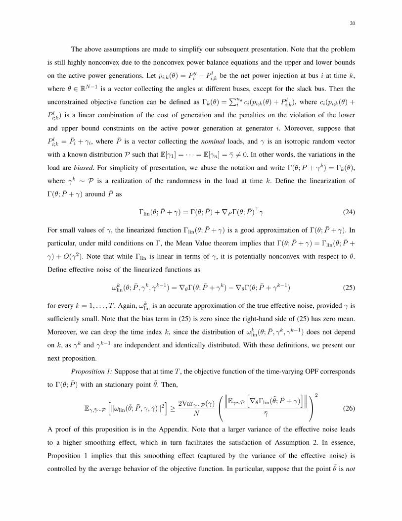
Proposition 1: Suppose that at time T , the objective function of the time-varying OPF corresponds

to Γ(θ; P ) with an stationary point θ. Then,

Eγ,γ∼P[‖ωlin(θ; P , γ, γ)‖2

]≥

2Varγ∼P(γ)

N

∥∥∥Eγ∼P [∇θΓlin(θ; P + γ)

]∥∥∥γ

2

(26)

A proof of this proposition is in the Appendix. Note that a larger variance of the effective noise leads

to a higher smoothing effect, which in turn facilitates the satisfaction of Assumption 2. In essence,

Proposition 1 implies that this smoothing effect (captured by the variance of the effective noise) is

controlled by the average behavior of the objective function. In particular, suppose that the point θ is not

21

a stationary point of the expected objective function. Therefore, we have∥∥∥Eγ∼P [∇θΓlin(θ; P + γ)

]∥∥∥ > 0,

and the above proposition implies that the generalized variance of the effective noise at θ increases with

the norm of the gradient of the expected function at θ, thereby leading to a higher smoothing effect of

the load variation and the elimination of the spurious local minima. This partly explains the high variance

of the effective noise at the local minimum of the objective function for the 2-bus system described in

Subsection IV-B, and the elimination of its spurious local minimum.

Based on our results, it is possible to eliminate the spurious local solutions in a point-wise OPF

problem by adding a synthetically generated noise to the load, thereby elevating the data variation in

the problem. This effect of random perturbation in the load values can be observed in Fig. 8c, where it

is shown that randomness in the load can eliminate the spurious local minimum and maximum, while

keeping the global minimum intact.

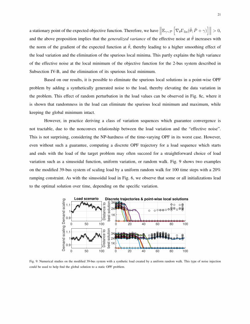
However, in practice deriving a class of variation sequences which guarantee convergence is

not tractable, due to the nonconvex relationship between the load variation and the “effective noise”.

This is not surprising, considering the NP-hardness of the time-varying OPF in its worst case. However,

even without such a guarantee, computing a discrete OPF trajectory for a load sequence which starts

and ends with the load of the target problem may often succeed for a straightforward choice of load

variation such as a sinusoidal function, uniform variation, or random walk. Fig. 9 shows two examples

on the modified 39-bus system of scaling load by a uniform random walk for 100 time steps with a 20%

ramping constraint. As with the sinusoidal load in Fig. 6, we observe that some or all initializations lead

to the optimal solution over time, depending on the specific variation.

0 50 100

0.9

1

1.1

Dem

and s

calin

g Load scenario

0 20 40 60 80 100

1K

2K

3K

Dis

tance to

best solu

tion

Discrete trajectories & point-wise local solutions

0 50 100

0.9

1

1.1

Dem

and s

calin

g

0 20 40 60 80 100

1K

2K

3K

Dis

tance to

best solu

tion

Fig. 9: Numerical studies on the modified 39-bus system with a synthetic load created by a uniform random walk. This type of noise injection

could be used to help find the global solution to a static OPF problem.

22

V. CONCLUSION

This paper studies time-varying optimal power flow (OPF) problems, in which a set of optimiza-

tion problems are solved sequentially due to load data variation over time. The solution to each OPF is

obtained using local search initialized at the solution to the previous OPF. We offer a case study on a

39-bus system under California data, where the OPF at the initial time has 16 locally optimal solutions

leading to 16 solution trajectories. We show that all trajectories converge to the best solution trajectory,

even though OPF has many local minima at most times. To understand this highly desirable property,

we introduce the notions of escaping period and tracking period, examine the role of data variation and

the easiest intermediate problem, study the behavior of the time-varying OPF during the escaping period

via a backward-in-time mapping, and relate it to SGD algorithm. By modeling the data variation as a

biased noise, we prove that enough data variation enables escaping poor solutions of time-varying OPF

over time.

REFERENCES

[1] J. Mulvaney-Kemp, S. Fattahi, and J. Lavaei, “Load variation enables escaping poor solutions of time-varying optimal

power flow,” IEEE Power & Energy Society General Meeting, 2020.

[2] J. A. Momoh, Electric Power System Applications of Optimization. Boca Raton: CRC Press, /12/19 2017.

[3] R. Baldick, Applied optimization: formulation and algorithms for engineering systems. Cambridge University Press, 2006.

[4] W. A. Bukhsh, A. Grothey, K. I. M. McKinnon, and P. A. Trodden, “Local solutions of the optimal power flow problem,”

IEEE Transactions on Power Systems, vol. 28, no. 4, pp. 4780–4788, Nov 2013.

[5] R. Y. Zhang, J. Lavaei, and R. Baldick, “Spurious local minima in power system state estimation,” IEEE Transactions on

Control of Network Systems, vol. 6, no. 3, pp. 1086–1096, 2019.

[6] R. Y. Zhang, S. Sojoudi, and J. Lavaei, “Sharp restricted isometry bounds for the inexistence of spurious local minima in

nonconvex matrix recovery,” Journal of Machine Learning research, 2019.

[7] C. Coffrin, H. L. Hijazi, and P. Van Hentenryck, “The QC relaxation: A theoretical and computational study on optimal

power flow,” IEEE Transactions on Power Systems, vol. 31, no. 4, pp. 3008–3018, 2015.

[8] B. Kocuk, S. S. Dey, and X. A. Sun, “Strong SOCP relaxations for the optimal power flow problem,” Operations Research,

vol. 64, no. 6, pp. 1177–1196, 2016.

[9] J. Lavaei and S. H. Low, “Zero duality gap in optimal power flow problem,” IEEE Transactions on Power Systems, vol. 27,

no. 1, pp. 92–107, 2012.

[10] S. Sojoudi and J. Lavaei, “Exactness of semidefinite relaxations for nonlinear optimization problems with underlying graph

structure,” SIAM Journal on Optimization, vol. 24, no. 4, pp. 1746–1778, 2014.

[11] C. Josz, J. Maeght, P. Panciatici, and J. C. Gilbert, “Application of the moment-sos approach to global optimization of the

opf problem,” IEEE Transactions on Power Systems, vol. 30, no. 1, pp. 463–470, 2014.

[12] D. Kourounis, A. Fuchs, and O. Schenk, “Toward the next generation of multiperiod optimal power flow solvers,” IEEE

Transactions on Power Systems, vol. 33, no. 4, pp. 4005–4014, 2018.

[13] A. Gopalakrishnan, A. U. Raghunathan, D. Nikovski, and L. T. Biegler, “Global optimization of multi-period optimal

power flow,” in 2013 American Control Conference, June 2013, pp. 1157–1164.

23

[14] S. Gill, I. Kockar, and G. W. Ault, “Dynamic optimal power flow for active distribution networks,” IEEE Transactions on

Power Systems, vol. 29, no. 1, pp. 121–131, Jan 2014.

[15] A. Costa and A. S. Costa, “Energy and ancillary service dispatch through dynamic optimal power flow,” Electric Power

Systems Research, vol. 77, no. 8, pp. 1047 – 1055, 2007.

[16] Y. Tang, K. Dvijotham, and S. Low, “Real-time optimal power flow,” IEEE Transactions on Smart Grid, vol. 8, no. 6, pp.

2963–2973, 2017.

[17] E. Dall’Anese and A. Simonetto, “Optimal power flow pursuit,” IEEE Transactions on Smart Grid, vol. 9, no. 2, pp.

942–952, March 2018.

[18] S. Bolognani, G. Cavraro, and S. Zampieri, A Distributed Feedback Control Approach to the Optimal Reactive Power Flow

Problem. Heidelberg: Springer International Publishing, 2013, pp. 259–277.

[19] L. Gan and S. H. Low, “An online gradient algorithm for optimal power flow on radial networks,” IEEE Journal on

Selected Areas in Communications, vol. 34, no. 3, pp. 625–638, March 2016.

[20] S. Fattahi, C. Josz, R. Mohammadi, J. Lavaei, and S. Sojoudi, “Absence of spurious local trajectories in time-varying

optimization,” 2019. [Online]. Available: https://lavaei.ieor.berkeley.edu/Time Varing 2019 1.pdf

[21] M. H. Amini, J. Mohammadi, and S. Kar, “Distributed holistic framework for smart city infrastructures: Tale of

interdependent electrified transportation network and power grid,” IEEE Access, vol. 7, pp. 157 535–157 554, 2019.

[22] R. D. Zimmerman, C. E. Murillo-Sanchez, and R. J. Thomas, “Matpower: Steady-state operations, planning, and analysis

tools for power systems research and education,” IEEE Transactions on Power Systems, vol. 26, no. 1, pp. 12–19, Feb

2011.

[23] “California ISO OASIS.” [Online]. Available: http://oasis.caiso.com/

[24] O. Massicot and J. Marecek, “On-line non-convex constrained optimization,” arXiv preprint arXiv:1909.07492, 2019.

[25] Y. Tang, “Time-varying optimization and its application to power system operation,” Ph.D. dissertation, California Institute

of Technology, 2019.

[26] D. Bertsekas, Nonlinear Programming, 3rd ed. Belmont, Mass.: Athena Scientific, 2016.

[27] C. B. Do, Q. V. Le, and C. S. Foo, “Proximal regularization for online and batch learning,” ICML, 2009.

[28] R. Kleinberg, Y. Li, and Y. Yuan, “An alternative view: When does SGD escape local minima?” arXiv preprint

arXiv:1802.06175, 2018.

[29] J. Chen and R. Luss, “Stochastic gradient descent with biased but consistent gradient estimators,” arXiv preprint

arXiv:1807.11880, 2018.

[30] E. K. Ryu and S. Boyd, “Stochastic proximal iteration: a non-asymptotic improvement upon stochastic gradient descent,”

http:// stanford.edu/∼boyd/papers/spi.html, 2017.

24

APPENDIX

PROOF OF THEOREM 1

For simplicity of notation, we reverse the order of the time steps, changing T − t to t. Then, the

dynamics (13) can be written as

zt = zt−1 + η∇Γ0(zt−1) + η

t−1∑k=1

ζk(zt−1)− ηt−1∑k=1

ωk (27)

We will extensively use the following sequences of intermediate points in our analysis:

yt = zt + η∇Γ0(zt) + η

t∑k=1

ζk(zt) (28)

yt = yt − ηt−1∑k=1

ωk (29)

It is easy to verify that the above definitions together with (27) gives rise to the following recursive

equation:

yt =yt−1 − ηt−1∑k=1

ωk + η∇Γ0

(yt−1 − η

t−1∑k=1

ωk

)+ η

t∑k=1

ζk

(yt−1 − η

t−1∑k=1

ωk

)(30)

which in turn implies

yt =yt−1 − ηωt−1 + η∇Γ0 (yt−1 − ηωt−1) + η

t∑k=1

ζk (yt−1 − ηωt−1) (31)

Define the filtration Ft−1 = σ{ω1, . . . , ωt−2} and the following stochastic process:

Gt = (1 + λ)−t(‖yt − z∗‖2 − 2(b1 + b2t+ b3t

2)

λ

)(32)

where b1 := 2η3r2L, b2 := 2η3r2l, and b3 := 4η2r2(1+2λ)2

λ . Our next lemma provides a lower bound on

E[‖yt − z∗‖2|Ft−1] in terms of ‖yt−1 − z∗‖2.

Lemma 1: The following inequality holds:

E[‖yt−z∗‖2|Ft−1] ≥(1+λ)‖yt−1−z∗‖2 − (b1+b2t+b3t2) (33)

25

Proof. Based on (31), one can write

E[‖yt − z∗‖2|Ft−1]

=E[‖yt−1 − z∗ − ηωt−1 + η∇Γ0 (yt−1 − ηωt−1) + η

t∑k=1

ζk (yt−1 − ηωt−1) ‖2|Ft−1]

≥‖yt−1 − z∗‖2 + η2E[‖ωt−1‖2|Ft−1] + E[‖η∇Γ0(yt−1−ηωt−1) + η

t∑k=1

ζk(yt−1−ηωt−1)‖2|Ft−1]

−2ηE[〈ηωt−1,∇Γ0(yt−1 − ηωt−1)〉|Ft−1]−2ηE[〈ηωt−1,

t∑k=1

Γ0(yt−1 − ηωt−1)〉|Ft−1]

+2η〈z∗ − yt−1,−∇E[Γ0(yt−1 − ηωt−1)|Ft−1]〉+2η〈z∗ − yt−1,−t∑

k=1

E[ζk(yt−1 − ηωt−1)|Ft−1]〉

≥‖yt−1 − z∗‖2

−2ηE[〈ηωt−1,∇Γ0(yt−1 − ηωt−1)〉|Ft−1]︸ ︷︷ ︸A

−2ηE[〈ηωt−1,

t∑k=1

Γ0(yt−1 − ηωt−1)〉|Ft−1]︸ ︷︷ ︸B

+2η〈z∗ − yt−1,−∇E[Γ0(yt−1 − ηωt−1)|Ft−1]〉︸ ︷︷ ︸C

+2η〈z∗ − yt−1,−t∑

k=1

E[ζk(yt−1 − ηωt−1)|Ft−1]︸ ︷︷ ︸D

〉

(34)

Next, we will provide a separate lower bound for each term in the above inequality. First, due to

Assumption 3, we have

C ≥ 2ηc‖yt−1 − z∗‖2 (35)

and

D ≥ −2ηc′‖yt−1 − z∗‖2 (36)

Furthermore, one can write

A = −2ηE[〈ηωt−1,∇Γ0(yt−1 − ηωt−1)−∇Γ0(yt−1)〉|Ft−1]

≥ −2ηE[‖ηωt−1‖‖Γ0(yt−1 − ηωt−1)−∇Γ0(yt−1)‖|Ft−1]

≥ −2η3r2L (37)

where the first equality is due to the fact that E[〈ηωt−1,Γ0(yt−1)〉|Ft−1] = 0. Similarly, we can write

B ≥ −2η3r2lt (38)

26

This implies that

E[‖yt − z∗‖2|Ft−1] ≥(1 + 2η(c− c′))‖yt−1 − z∗‖2 − 2η3r2(L+ lt)

=(1 + 2λ)‖yt−1 − z∗‖2 − (b1 + b2t) (39)

This together with the definition of yt−1 gives rise to the following chain of inequalities

E[‖yt − z∗‖2|Ft−1] ≥(1 + 2λ)

∥∥∥∥∥yt−1 − ηt−2∑k=1

ωk − z∗

∥∥∥∥∥2

− (b1 + b2t)

≥(1 + 2λ)‖yt−1 − z∗‖2−2(1 + 2λ)‖yt−1 − z∗‖

∥∥∥∥∥ηt−2∑k=1

ωk

∥∥∥∥∥− (b1 + b2t)

≥(1+2λ)‖yt−1−z∗‖2−2ηr(1+2λ)t‖yt−1−z∗‖−(b1+b2t) (40)

Now we consider two cases:

- If ‖yt−1 − z∗‖ ≥ 2ηr(1+2λ)tλ , then one can write

E[‖yt−z∗‖2|Ft−1] ≥ (1+λ)‖yt−1−z∗‖2−(b1+b2t) (41)

- If ‖yt−1 − z∗‖ < 2ηr(1+2λ)tλ , then one can write

E[‖yt − z∗‖2|Ft−1] ≥(1 + 2λ)‖yt−1 − z∗‖2 − 4η2r2(1 + 2λ)2t2

λ−(b1 + b2t) (42)

Combining the above two inequalities leads to

E[‖yt − z∗‖2|Ft−1] ≥(1 + λ)‖yt−1 − z∗‖2 − (b1 + b2t+ b3t2) (43)

�

The next lemma is at the crux of our proof for Theorem 1.

Lemma 2: The following two statements hold:

1) Gt is a submartingale with a vanishing drift. More precisely, it satisfies the following inequality

E[Gt|Ft−1]≥Gt−1−(1+λ)−(t−1)

(2b2 + 2b3(2t−1)

λ

)(44)

2) E[Gt] ≥ G0 −(

2λ + 2

λ2

)b2 −

(4λ

(1 + 1

λ

)2)b3

Proof. One can write

E[Gt|Ft−1] = (1 + λ)−t(E[‖yt − z∗‖2|Ft−1]− 2(b1 + b2t+ b3t

2)

λ

)(45)

27

Invoking Lemma 1 leads to

E[Gt|Ft−1] ≥(1 + λ)−t(

(1 + λ)‖yt−1 − z∗‖2 − (b1 + b2t+ b3t2)− 2(b1 + b2t+ b3t

2)

λ

)=(1 + λ)−(t−1)‖yt−1 − z∗‖2 − (1 + λ)−(t−1)

(2(b1 + b2t+ b3t

2)

λ

)=(1 + λ)−(t−1)‖yt−1 − z∗‖2 − (1 + λ)−(t−1)

(2(b1 + b2(t− 1) + b3(t− 1)2)

λ

)− (1 + λ)−(t−1)

(2(b2 + b3(2t− 1))

λ

)=Gt−1 − (1 + λ)−(t−1)

(2b2 + 2b3(2t− 1)

λ

)(46)

This completes the proof of the first part. To prove the second part, we use the result of the first part

together with the tower property of the expectation to write

E[Gt] ≥G0 −

(2b2λ

t−1∑k=0

(1 + λ)−k

)︸ ︷︷ ︸

A

−

(4b3λ

t−1∑k=0

(k + 1)(1 + λ)−k

)︸ ︷︷ ︸

B

(47)

It is easy to verify that

A ≤(

2

λ+

2

λ2

)b2, B ≤

(4

λ

(1 +

1

λ

)2)b3 (48)

This completes the proof. �

Proof of Theorem 1: From the second statement of Lemma 2, one can write

‖y0 − z∗‖2 ≤(

2

λ+

2

λ2

)b2 +

(4

λ

(1 +

1

λ

)2)b3 + (1 + λ)−(t−1) E[‖yt−1 − z∗‖2] (49)

On the other hand, one can write

E[‖zt − z∗‖2] = E[‖yt−1 − z∗ − ηt−1∑k=1

ωk‖2] (50)

≥ E[‖yt−1 − z∗‖2]− 2ηrtE[‖yt−1 − z∗‖]

Inequality (50) together with some simple algebra reveals that

E[‖yt−1 − z∗‖2] ≤ 2E[‖zt − z∗‖2] + 16η2r2t2 (51)

Combining the above inequality with (49) results in

‖y0 − z∗‖2 ≤(

2

λ+

2

λ2

)b2 +

(4

λ

(1 +

1

λ

)2)b3 + 2 (1 + λ)−(t−1) E[‖zt − z∗‖2] + 16η2r2t2(1 + λ)−(t−1)

(52)

28

Finally, it only remains to characterize the relationship between ‖y0−z∗‖2 and ‖z0−z∗‖2. To this goal,

one can write

‖y0 − z∗‖2 = ‖z0 − z∗ + η∇f0(z0)‖2

≥‖z0 − z∗‖2 − 2η〈z0 − z∗, η∇f0(z0)〉

=‖z0 − z∗‖2 − 2η〈z0 − z∗, η∇f0(z0)− η∇f0(z∗)〉

≥‖z0 − z∗‖2 − 2η2‖z0 − z∗‖‖∇f0(z0)−∇f0(z∗)‖

≥(1− 2η2L)‖z0 − z∗‖2 (53)

where the last inequality is due to Assumption 1. Combining (53) with (52) concludes the proof. �

APPENDIX

PROOF OF PROPOSITION 1

Due to the definition of Γlin(θ; P + γ) in (24), one can write

Eγ∼P[∇θΓlin(θ; P+γ)

]=

N∑i=1

∇pi(θ)ci(pi(θ)+Pi)∇θpi(θ) +

N∑i=1

∇pi(θ)∇Pici(pi(θ)+Pi)E[γi]∇θpi(θ)

=

N∑i=1

∇pi(θ)∇Pici(pi(θ)+Pi)E[γi]∇θpi(θ) (54)

where the second equality follows from the assumption ∇θΓlin(θ; P ) = 0. Let us define the vector

vi = ∇pi(θ)∇Pici(pi(θ)+Pi)∇θpi(θ). Therefore, one can write(N∑i=1

‖vi‖

)2

≥

∥∥∥∥∥N∑i=1

vi

∥∥∥∥∥2

=

∥∥∥Eγ∼P [∇θΓlin(θ; P+γ)]∥∥∥2

γ2(55)

On the other hand, a simple calculation reveals that

ωklin(θ; P , γ, γ) =∇θΓ(θ; P + γ)−∇θΓ(θ; P + γ)

=

N∑i=1

∇pi(θ)∇Pici(pi(θ)+Pi)(γi − γi)∇θpi(θ) (56)

29

Upon defining the matrix V = [v1, v2, . . . , vN ], one can verify that ωklin(θ; P , γ, γ) = V (γ − γ), which

implies that

Eγ,γ∼P [‖ωlin(θ; P , γ, γ)‖2] = Eγ,γ∼P[‖V (γ − γ)‖2

]= 2Varγ∼P(γ)trace

(V V >

)= 2Varγ∼P(γ)trace

(V >V

)= 2Varγ∼P(γ)

(N∑i=1

‖vi‖2)

(57)

This implies that

Eγ,γ∼P [‖ωlin(θ; P , γ, γ)‖2] ≥2Varγ∼P(γ)

N

(N∑i=1

‖vi‖

)2

The above inequality combined with (55) completes the proof. �