Embed Size (px)
Citation preview
Modified: August 22, 2011
Exponential Smoothing Forecasting Using SCAB34S and SCA WorkBench
William J. Lattyak
Scientific Computing Associates Corp.
Houston H. Stokes
Department of Economics
University of Illinois at Chicago
1
Table of Contents
1. SUPPORTED FORECASTING METHODS ................................................................................................ 3
1.1 Naïve No Change Extrapolation (NCE)......................................................................................................... 5 1.2 Simple Exponential Smoothing with No Trend (N_N) ................................................................................ 5 1.3 Holts Exponential Smoothing with Additive Trend (A_N) .......................................................................... 6 1.4 Pegels Exponential Smoothing with Multiplicative Trend (M_N) .............................................................. 7 1.5 Modified Holts Exponential Smoothing with Damped Additive Trend (DA_N) ....................................... 8 1.6 Modified Pegels Exponential Smoothing with Damped Multiplicative Trend (DM_N) ............................ 8 1.7 Additive Seasonal Exponential Smoothing with No Trend (N_A) .............................................................. 9 1.8 Additive Seasonal Exponential Smoothing with Additive Trend (A_A) ..................................................... 9 1.9 Additive Seasonal Exponential Smoothing with Multiplicative Trend (M_A) ........................................ 10 1.10 Additive Seasonal Exponential Smoothing with Damped Additive Trend (DA_A) .............................. 11 1.11 Additive Seasonal Exponential Smoothing with Damped Multiplicative Trend (DM_A) .................... 11 1.12 Multiplicative Seasonal Exponential Smoothing with No Trend (N_M) ................................................ 12 1.13 Multiplicative Seasonal Exponential Smoothing with Additive Trend (A_M) ...................................... 12 1.14 Multiplicative Seasonal Exponential Smoothing with Multiplicative Trend (M_M) ............................ 13 1.15 Multiplicative Seasonal Exponential Smoothing with Damped Additive Trend (DA_M) .................... 13 1.16 Multiplicative Seasonal Exponential Smoothing with Damped Multiplicative Trend (DM_M) ......... 14 1.17 Croston Intermittent Demand Method (CROSTON) .............................................................................. 14 1.18 Modified Croston Intermittent Demand Method by Syntetos and Boylan (MCROSTON) ................. 15 1.19 Modified Crostons Intermittent Demand Method by Teunter and Sani (VCROSTON) ...................... 15
2 SCA WORKBENCH: A GRAPHICAL USER INTERFACE .................................................................... 16
2.1 Model tab ....................................................................................................................................................... 16 2.2 Options tab ..................................................................................................................................................... 20 2.4 Results tab ...................................................................................................................................................... 22 2.5 Graphs tab ..................................................................................................................................................... 24
3. EXAMPLES OF EXPONENTIAL SMOOTHING USING SCA WORKBENCH .................................. 25
3.1 Forecasting Durable Goods with Multivariate Trend Using Pagel’s Method .......................................... 25 3.1.1 Specification of the (M_N) Method for Durable Goods Inventory Forecasting .................................. 27 3.1.2 Exponential Smoothing Options for the Durable Goods Inventory Example ...................................... 28 3.1.3 Forecasting Result for the Durable Goods Inventory Example ............................................................ 30
3.2 Forecasting Seasonal Airline Passenger Load based on Automatic Method Selection ........................... 33 3.2.1 Specifying a Mult-Method Competition to Select a Forecasting Method for Passenger Load ............. 34 3.2.2 Result of the Multi-Method Scenario for the Airline Passenger Load Example ................................... 36
3.3 Forecasting Intermittent Demand based on Automatic Method Selection ............................................... 40 3.2.1 Specifying a Mult-Method Competition to Select a Forecasting Method for the Intermittent Demand
Example 41 3.3.2 Result of the Multi-Method Scenario for the Intermittent Demand Example ....................................... 43
4. DETAILED DESCRIPTION OF THE SMOOTH ROUTINE IN SCAB34S ........................................... 47
Usage: ............................................................................................................................................................... 47 Required subroutine arguments: ..................................................................................................................... 47 Optional keywords and associated arguments: ................................................................................................ 47 Variables created in SMOOTH subroutine call: ............................................................................................. 49
5. A DETAILED DESCRIPTION OF CUSTOMIZABLE SUBROUTINES USED IN THE
EXPONENTIAL SMOOTHING APPLICATION ....................................................................................... 51
5.1 INIEXPSM User Program ........................................................................................................................ 51 Usage: ............................................................................................................................................................... 51 Initialized Global Arguments: .......................................................................................................................... 51
5.2 SETEXPSM User Program ....................................................................................................................... 53 Usage: ............................................................................................................................................................... 54

2
5.3 RUNEXPSM User Program...................................................................................................................... 54 Usage: ............................................................................................................................................................... 54
5.4 DSPEXPSM User Program ....................................................................................................................... 54 Usage: ............................................................................................................................................................... 54
5.5 GRFEXPS1 User Program........................................................................................................................ 54 Usage: ............................................................................................................................................................... 54
5.6 AUTOEXP1 User Program ....................................................................................................................... 55 Usage: ............................................................................................................................................................... 55
5.7 EXPSM User Subroutine .......................................................................................................................... 55 Usage: ............................................................................................................................................................... 55 Required global arguments: ............................................................................................................................. 57 Required subroutine arguments: ..................................................................................................................... 57 Example: ........................................................................................................................................................... 59
6. EXAMPLES OF SCAB34S COMMAND FILES FOR EXPONENTIAL SMOOTHING.................. 60 6.1 SCAB34S Commands Generated for the Durable Goods Inventory Example .................................... 60 6.2 SCAB34S Commands for the Seasonal Airline Passenger Load Example ........................................... 61 6.3 SCAB34S Commands for the Intermittent Demand Forecasting Example.......................................... 63 6.4 SCAB34S Commands Used to Display Graphs in the Examples ........................................................... 65
REFERENCES .................................................................................................................................................... 67
3
Exponential Smoothing Forecasting Using SCAB34S and SCA WorkBench
In this document, we discuss exponential smoothing forecasting provided by the B34S®
ProSeries Econometric System and SCAB34S software products. We also discuss the SCA
WorkBench companion product and its user interface to shell exponential smoothing forecasting
and exploration in the B34S program suite. There are 19 forecasting methods to choose from
accommodating time series with and without trend, time series with and without seasonality, and
time series with continuous and interrupted (intermittent demand) patterns. A historical
overview and description of the various exponential smoothing methods supported here can be
found in Gardner Jr., E.S. (1985, 2006).
SCAB34S provides a subset of the capabilities in the B34S® ProSeries Econometric System
and we refer to these products interchangeably within this document. The SCA WorkBench
product is a companion to the SCA Statistical System and SCAB34S software, providing a
graphical user interface for exponential smoothing forecasting applications.
The SCAB34S product provides a number of procedures to perform common data
manipulation tasks, organizational tasks, and statistical/econometric analysis tasks. It also
contains a comprehensive matrix programming language that may be used to customize
procedures. No attempt will be made to cover all features of the SCAB34S product in this
document nor the full range of applications that may be solved using the B34S matrix
programming facilities.1 Instead, we shall exclusively use the graphical user interface of SCA
WorkBench to specify, estimate, and forecast exponential smoothing methods in SCAB34S.
SCA WorkBench automatically builds the command script executed in the SCAB34S product
based on menu selections. The command script is executed in the SCAB34S engine and the
results are read back into WorkBench for examination. The user may save the program file and
modify the command script to address additional analysis requirements that may arise.
This is a pre-released version of the exponential smoothing application environment in SCA
WorkBench. The application environment is currently focused on exponential smoothing
exploration; processing one series at a time. Here, users can apply a specific exponential
smoothing method or run a competition of multiple exponential smoothing methods on a single
series to determine the best performing method for forecasting. The official release of the
exponential smoothing application environment will allow users to handle large numbers of time
series in an automated fashion.
1. SUPPORTED FORECASTING METHODS
Traditional forecasting methods were developed from statistical theory or from empirical
experiences. However, a common characteristic is that forecasts are based essentially on
smoothing (averaging) past values of a time series using some type of weighting scheme. Naïve
1 The text, Specifying and Diagnostically Testing Econometric Models, by Houston H. Stokes Greenwood
Press (1997) documents the basic B34S capability. A comprehensive document covering the B34S matrix command
facilities is under preparation.
4
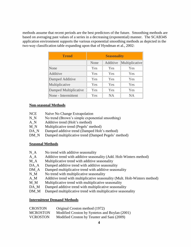
methods assume that recent periods are the best predictors of the future. Smoothing methods are
based on averaging past values of a series in a decreasing (exponential) manner. The SCAB34S
application environment supports the various exponential smoothing methods as depicted in the
two-way classification table expanding upon that of Hyndman et al., 2002:
Trend Seasonality
None Additive Multiplicative
None Yes Yes Yes
Additive Yes Yes Yes
Damped Additive Yes Yes Yes
Multiplicative Yes Yes Yes
Damped Multiplicative Yes Yes Yes
None - Intermittent Yes NA NA
Non-seasonal Methods
NCE Naïve No Change Extrapolation
N_N No trend (Brown’s simple exponential smoothing)
A_N Additive trend (Holt’s method)
M_N Multiplicative trend (Pegels’ method)
DA_N Damped additive trend (Damped Holt’s method)
DM_N Damped multiplicative trend (Damped Pegels’ method)
Seasonal Methods
N_A No trend with additive seasonality
A_A Additive trend with additive seasonality (Add. Holt-Winters method)
M_A Multiplicative trend with additive seasonality
DA_A Damped additive trend with additive seasonality
DM_A Damped multiplicative trend with additive seasonality
N_M No trend with multiplicative seasonality
A_M Additive trend with multiplicative seasonality (Mult. Holt-Winters method)
M_M Multiplicative trend with multiplicative seasonality
DA_M Damped additive trend with multiplicative seasonality
DM_M Damped multiplicative trend with multiplicative seasonality
Intermittent Demand Methods
CROSTON Original Croston method (1972)
MCROSTON Modified Croston by Syntetos and Boylan (2001)
VCROSTON Modified Croston by Teunter and Sani (2009)
5
The various forecasting methods are described in more detail in the subsections below.
1.1 Naïve No Change Extrapolation (NCE)
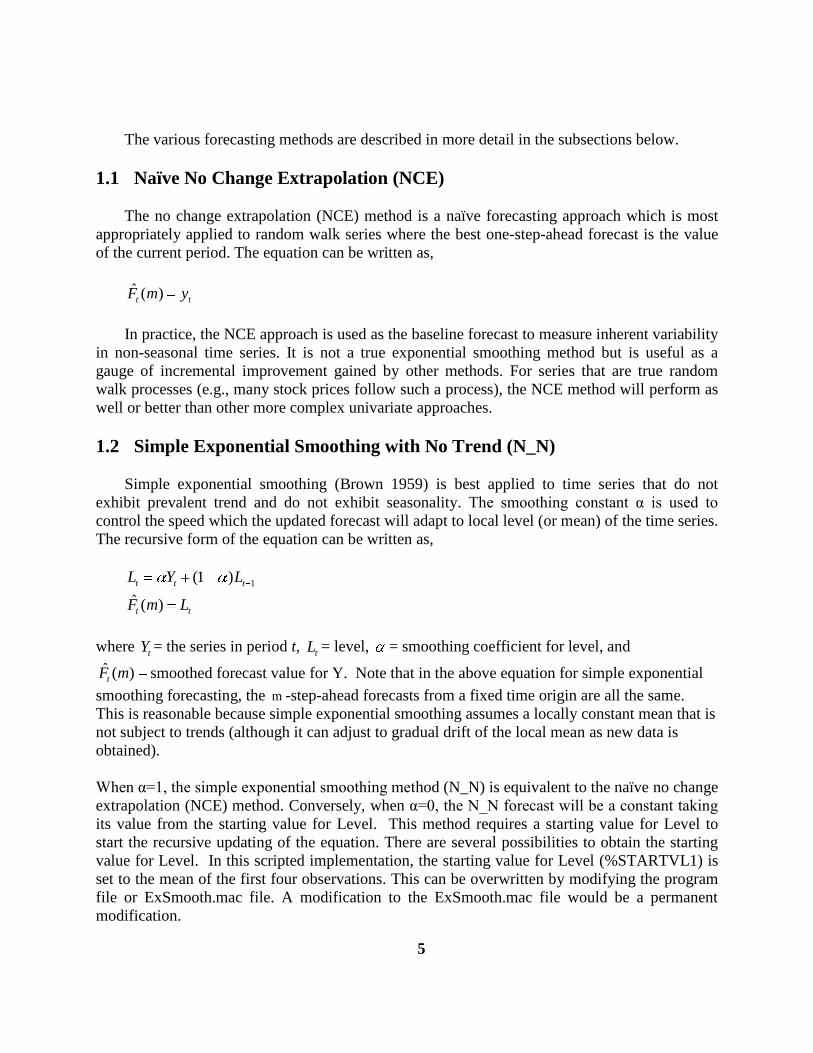
The no change extrapolation (NCE) method is a naïve forecasting approach which is most
appropriately applied to random walk series where the best one-step-ahead forecast is the value
of the current period. The equation can be written as,
ˆ ( )t tF m y
In practice, the NCE approach is used as the baseline forecast to measure inherent variability
in non-seasonal time series. It is not a true exponential smoothing method but is useful as a
gauge of incremental improvement gained by other methods. For series that are true random
walk processes (e.g., many stock prices follow such a process), the NCE method will perform as
well or better than other more complex univariate approaches.
1.2 Simple Exponential Smoothing with No Trend (N_N)
Simple exponential smoothing (Brown 1959) is best applied to time series that do not
exhibit prevalent trend and do not exhibit seasonality. The smoothing constant α is used to
control the speed which the updated forecast will adapt to local level (or mean) of the time series.
The recursive form of the equation can be written as,
1(1 )
ˆ ( )
t t t
t t
L Y L
F m L
where tY = the series in period t,
tL = level, = smoothing coefficient for level, and
ˆ ( )tF m smoothed forecast value for Y. Note that in the above equation for simple exponential
smoothing forecasting, the m -step-ahead forecasts from a fixed time origin are all the same.
This is reasonable because simple exponential smoothing assumes a locally constant mean that is
not subject to trends (although it can adjust to gradual drift of the local mean as new data is
obtained).
When α=1, the simple exponential smoothing method (N_N) is equivalent to the naïve no change
extrapolation (NCE) method. Conversely, when α=0, the N_N forecast will be a constant taking
its value from the starting value for Level. This method requires a starting value for Level to
start the recursive updating of the equation. There are several possibilities to obtain the starting
value for Level. In this scripted implementation, the starting value for Level (%STARTVL1) is
set to the mean of the first four observations. This can be overwritten by modifying the program
file or ExSmooth.mac file. A modification to the ExSmooth.mac file would be a permanent
modification.
6
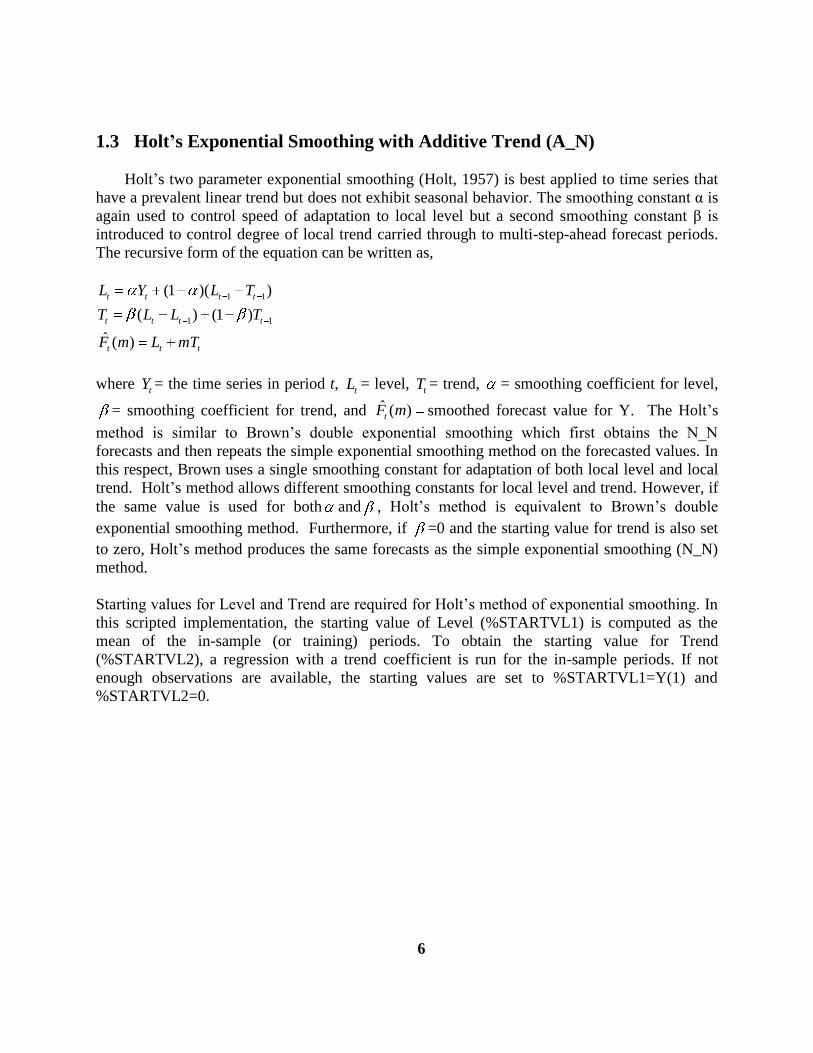
1.3 Holt’s Exponential Smoothing with Additive Trend (A_N)
Holt’s two parameter exponential smoothing (Holt, 1957) is best applied to time series that
have a prevalent linear trend but does not exhibit seasonal behavior. The smoothing constant α is
again used to control speed of adaptation to local level but a second smoothing constant β is
introduced to control degree of local trend carried through to multi-step-ahead forecast periods.
The recursive form of the equation can be written as,
1 1
1 1
(1 )( )
( ) (1 )
ˆ ( )
t t t t
t t t t
t t t
L Y L T
T L L T
F m L mT
where tY = the time series in period t,
tL = level, tT = trend, = smoothing coefficient for level,
= smoothing coefficient for trend, and ˆ ( )tF m smoothed forecast value for Y. The Holt’s
method is similar to Brown’s double exponential smoothing which first obtains the N_N
forecasts and then repeats the simple exponential smoothing method on the forecasted values. In
this respect, Brown uses a single smoothing constant for adaptation of both local level and local
trend. Holt’s method allows different smoothing constants for local level and trend. However, if
the same value is used for both and , Holt’s method is equivalent to Brown’s double
exponential smoothing method. Furthermore, if =0 and the starting value for trend is also set
to zero, Holt’s method produces the same forecasts as the simple exponential smoothing (N_N)
method.
Starting values for Level and Trend are required for Holt’s method of exponential smoothing. In
this scripted implementation, the starting value of Level (%STARTVL1) is computed as the
mean of the in-sample (or training) periods. To obtain the starting value for Trend
(%STARTVL2), a regression with a trend coefficient is run for the in-sample periods. If not
enough observations are available, the starting values are set to %STARTVL1=Y(1) and
%STARTVL2=0.
7
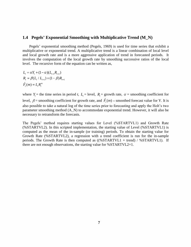
1.4 Pegels’ Exponential Smoothing with Multiplicative Trend (M_N)
Pegels’ exponential smoothing method (Pegels, 1969) is used for time series that exhibit a
multiplicative or exponential trend. A multiplicative trend is a linear combination of local level
and local growth rate and is a more aggressive application of trend in forecasted periods. It
involves the computation of the local growth rate by smoothing successive ratios of the local
level. The recursive form of the equation can be written as,
1 1
1 1
(1 )( )
( / ) (1 )
ˆ ( )
t t t t
t t t t
m
t t t
L Y L R
R L L R
F m L R
where tY = the time series in period t,
tL = level, tR = growth rate, = smoothing coefficient for
level, = smoothing coefficient for growth rate, and ˆ ( )tF m smoothed forecast value for Y. It is
also possible to take a natural log of the time series prior to forecasting and apply the Holt’s two
parameter smoothing method (A_N) to accommodate exponential trend. However, it will also be
necessary to retransform the forecasts.
The Pegels’ method requires starting values for Level (%STARTVL1) and Growth Rate
(%STARTVL2). In this scripted implementation, the starting value of Level (%STARTVL1) is
computed as the mean of the in-sample (or training) periods. To obtain the starting value for
Growth Rate (%STARTVL2), a regression with a trend coefficient is run for the in-sample
periods. The Growth Rate is then computed as ((%STARTVL1 + trend) / %STARTVL1). If
there are not enough observations, the starting value for %STARTVL2=1.
8
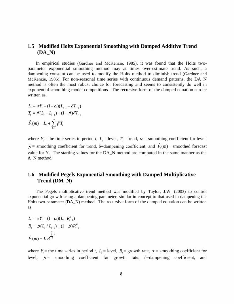
1.5 Modified Holts Exponential Smoothing with Damped Additive Trend
(DA_N)
In empirical studies (Gardner and McKenzie, 1985), it was found that the Holts two-
parameter exponential smoothing method may at times over-estimate trend. As such, a
dampening constant can be used to modify the Holts method to diminish trend (Gardner and
McKenzie, 1985). For non-seasonal time series with continuous demand patterns, the DA_N
method is often the most robust choice for forecasting and seems to consistently do well in
exponential smoothing model competitions. The recursive form of the damped equation can be
written as,
1 1
1 1
1
(1 )( )
( ) (1 )
ˆ ( )
t t t t
t t t t
mi
t t t
i
L Y L T
T L L T
F m L T
where tY = the time series in period t,
tL = level, tT = trend, = smoothing coefficient for level,
= smoothing coefficient for trend, δ=dampening coefficient, and ˆ ( )tF m smoothed forecast
value for Y. The starting values for the DA_N method are computed in the same manner as the
A_N method.
1.6 Modified Pegels Exponential Smoothing with Damped Multiplicative
Trend (DM_N)
The Pegels multiplicative trend method was modified by Taylor, J.W. (2003) to control
exponential growth using a dampening parameter, similar in concept to that used in dampening the
Holts two-parameter (DA_N) method. The recursive form of the damped equation can be written
as,
1
1 1
1 1
(1 )( )
( / ) (1 )
ˆ ( )
mi
i
t t t t
t t t t
t t t
L Y L R
R L L R
F m L R
where tY = the time series in period t,
tL = level, tR = growth rate, = smoothing coefficient for
level, = smoothing coefficient for growth rate, δ=dampening coefficient, and
9
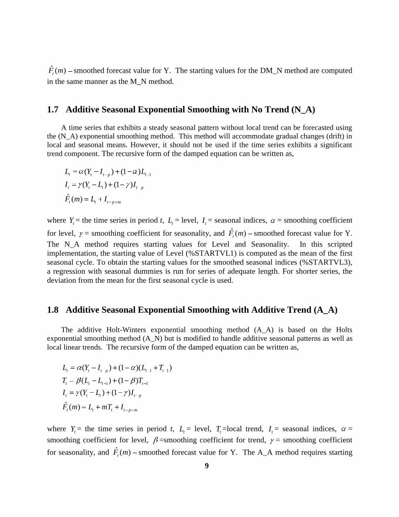
ˆ ( )tF m smoothed forecast value for Y. The starting values for the DM_N method are computed
in the same manner as the M_N method.
1.7 Additive Seasonal Exponential Smoothing with No Trend (N_A)
A time series that exhibits a steady seasonal pattern without local trend can be forecasted using
the (N_A) exponential smoothing method. This method will accommodate gradual changes (drift) in
local and seasonal means. However, it should not be used if the time series exhibits a significant
trend component. The recursive form of the damped equation can be written as,
1( ) (1 )
( ) (1 )
ˆ ( )
t t t p t
t t t t p
t t t p m
L Y I L
I Y L I
F m L I
where tY = the time series in period t,
tL = level, tI = seasonal indices, = smoothing coefficient
for level, = smoothing coefficient for seasonality, and ˆ ( )tF m smoothed forecast value for Y.
The N_A method requires starting values for Level and Seasonality. In this scripted
implementation, the starting value of Level (%STARTVL1) is computed as the mean of the first
seasonal cycle. To obtain the starting values for the smoothed seasonal indices (%STARTVL3),
a regression with seasonal dummies is run for series of adequate length. For shorter series, the
deviation from the mean for the first seasonal cycle is used.
1.8 Additive Seasonal Exponential Smoothing with Additive Trend (A_A)
The additive Holt-Winters exponential smoothing method (A_A) is based on the Holts
exponential smoothing method (A_N) but is modified to handle additive seasonal patterns as well as
local linear trends. The recursive form of the damped equation can be written as,
1 1
1 1
( ) (1 )( )
( ) (1 )
( ) (1 )
ˆ ( )
t t t p t t
t t t t
t t t t p
t t t t p m
L Y I L T
T L L T
I Y L I
F m L mT I
where tY = the time series in period t,
tL = level, tT =local trend,
tI = seasonal indices, =
smoothing coefficient for level, =smoothing coefficient for trend, = smoothing coefficient
for seasonality, and ˆ ( )tF m smoothed forecast value for Y. The A_A method requires starting
10
values for Level, Trend, and Seasonality. The starting value of Level (%STARTVL1) is
computed as the mean of the first seasonal cycle. The starting value for Trend (%STARTVL2) is
computed using regression with a trend component. To obtain the starting values for the
smoothed seasonal indices (%STARTVL3), a regression with seasonal dummies is run for series
of adequate length. For shorter series, the deviation from the mean for the first seasonal cycle is
used and trend is set to 0.
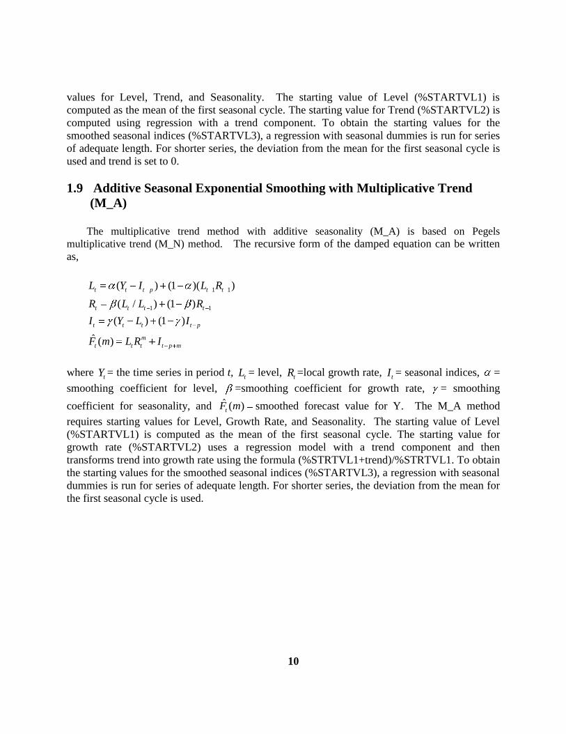
1.9 Additive Seasonal Exponential Smoothing with Multiplicative Trend
(M_A)
The multiplicative trend method with additive seasonality (M_A) is based on Pegels
multiplicative trend (M_N) method. The recursive form of the damped equation can be written
as,
1 1
1 1
( ) (1 )( )
( / ) (1 )
( ) (1 )
ˆ ( )
t t t p t t
t t t t
t t t t p
m
t t t t p m
L Y I L R
R L L R
I Y L I
F m L R I
where tY = the time series in period t,
tL = level, tR =local growth rate,
tI = seasonal indices, =
smoothing coefficient for level, =smoothing coefficient for growth rate, = smoothing
coefficient for seasonality, and ˆ ( )tF m smoothed forecast value for Y. The M_A method
requires starting values for Level, Growth Rate, and Seasonality. The starting value of Level
(%STARTVL1) is computed as the mean of the first seasonal cycle. The starting value for
growth rate (%STARTVL2) uses a regression model with a trend component and then
transforms trend into growth rate using the formula (%STRTVL1+trend)/%STRTVL1. To obtain
the starting values for the smoothed seasonal indices (%STARTVL3), a regression with seasonal
dummies is run for series of adequate length. For shorter series, the deviation from the mean for
the first seasonal cycle is used.
11
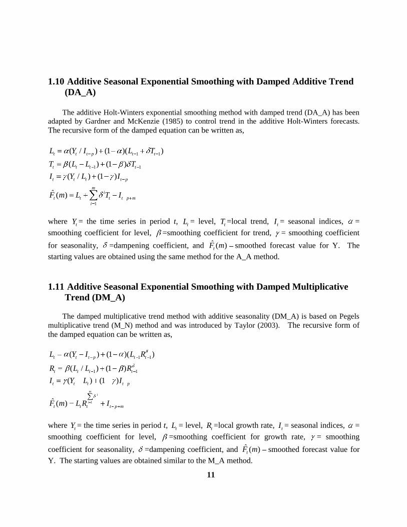
1.10 Additive Seasonal Exponential Smoothing with Damped Additive Trend
(DA_A)
The additive Holt-Winters exponential smoothing method with damped trend (DA_A) has been
adapted by Gardner and McKenzie (1985) to control trend in the additive Holt-Winters forecasts.
The recursive form of the damped equation can be written as,
1 1
1 1
1
( / ) (1 )( )
( ) (1 )
( / ) (1 )
ˆ ( )
t t t p t t
t t t t
t t t t p
mi
t t t t p m
i
L Y I L T
T L L T
I Y L I
F m L T I
where tY = the time series in period t,
tL = level, tT =local trend,
tI = seasonal indices, =
smoothing coefficient for level, =smoothing coefficient for trend, = smoothing coefficient
for seasonality, =dampening coefficient, and ˆ ( )tF m smoothed forecast value for Y. The
starting values are obtained using the same method for the A_A method.
1.11 Additive Seasonal Exponential Smoothing with Damped Multiplicative
Trend (DM_A)
The damped multiplicative trend method with additive seasonality (DM_A) is based on Pegels
multiplicative trend (M_N) method and was introduced by Taylor (2003). The recursive form of
the damped equation can be written as,
1
1 1
1 1
( ) (1 )( )
( / ) (1 )
( ) (1 )
ˆ ( )
mi
i
t t t p t t
t t t t
t t t t p
t t t t p m
L Y I L R
R L L R
I Y L I
F m L R I
where tY = the time series in period t,
tL = level, tR =local growth rate,
tI = seasonal indices, =
smoothing coefficient for level, =smoothing coefficient for growth rate, = smoothing
coefficient for seasonality, =dampening coefficient, and ˆ ( )tF m smoothed forecast value for
Y. The starting values are obtained similar to the M_A method.
12
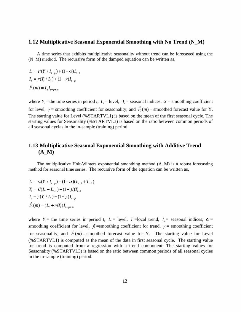
1.12 Multiplicative Seasonal Exponential Smoothing with No Trend (N_M)
A time series that exhibits multiplicative seasonality without trend can be forecasted using the
(N_M) method. The recursive form of the damped equation can be written as,
1( / ) (1 )
( / ) (1 )
ˆ ( )
t t t p t
t t t t p
t t t p m
L Y I L
I Y L I
F m L I
where
tY = the time series in period t, tL = level,
tI = seasonal indices, = smoothing coefficient
for level, = smoothing coefficient for seasonality, and ˆ ( )tF m smoothed forecast value for Y.
The starting value for Level (%STARTVL1) is based on the mean of the first seasonal cycle. The
starting values for Seasonality (%STARTVL3) is based on the ratio between common periods of
all seasonal cycles in the in-sample (training) period.
1.13 Multiplicative Seasonal Exponential Smoothing with Additive Trend
(A_M)
The multiplicative Holt-Winters exponential smoothing method (A_M) is a robust forecasting
method for seasonal time series. The recursive form of the equation can be written as,
1 1
1 1
( / ) (1 )( )
( ) (1 )
( / ) (1 )
ˆ ( ) ( )
t t t p t t
t t t t
t t t t p
t t t t p m
L Y I L T
T L L T
I Y L I
F m L mT I
where
tY = the time series in period t, tL = level,
tT =local trend, tI = seasonal indices, =
smoothing coefficient for level, =smoothing coefficient for trend, = smoothing coefficient
for seasonality, and ˆ ( )tF m smoothed forecast value for Y. The starting value for Level
(%STARTVL1) is computed as the mean of the data in first seasonal cycle. The starting value
for trend is computed from a regression with a trend component. The starting values for
Seasonality (%STARTVL3) is based on the ratio between common periods of all seasonal cycles
in the in-sample (training) period.
13
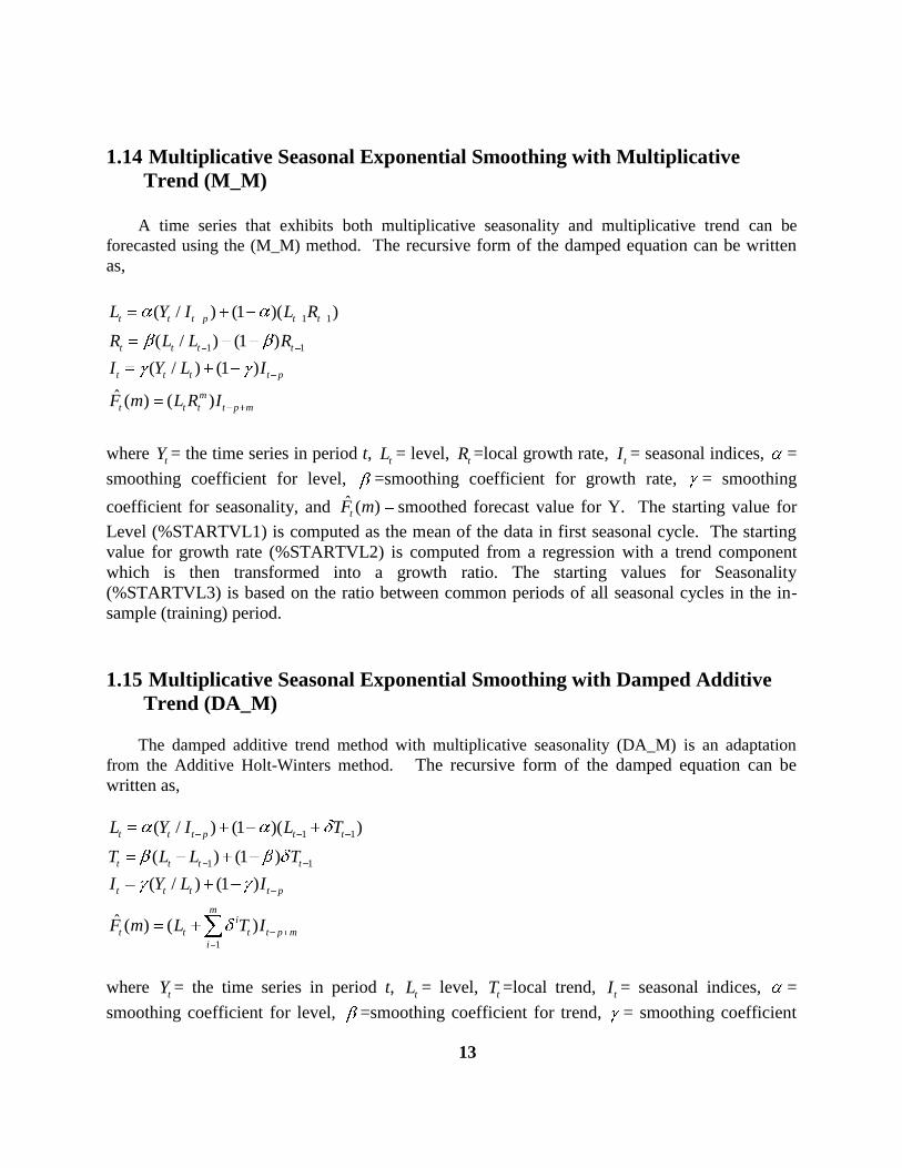
1.14 Multiplicative Seasonal Exponential Smoothing with Multiplicative
Trend (M_M)
A time series that exhibits both multiplicative seasonality and multiplicative trend can be
forecasted using the (M_M) method. The recursive form of the damped equation can be written
as,
1 1
1 1
( / ) (1 )( )
( / ) (1 )
( / ) (1 )
ˆ ( ) ( )
t t t p t t
t t t t
t t t t p
m
t t t t p m
L Y I L R
R L L R
I Y L I
F m L R I
where
tY = the time series in period t, tL = level,
tR =local growth rate, tI = seasonal indices, =
smoothing coefficient for level, =smoothing coefficient for growth rate, = smoothing
coefficient for seasonality, and ˆ ( )tF m smoothed forecast value for Y. The starting value for
Level (%STARTVL1) is computed as the mean of the data in first seasonal cycle. The starting
value for growth rate (%STARTVL2) is computed from a regression with a trend component
which is then transformed into a growth ratio. The starting values for Seasonality
(%STARTVL3) is based on the ratio between common periods of all seasonal cycles in the in-
sample (training) period.
1.15 Multiplicative Seasonal Exponential Smoothing with Damped Additive
Trend (DA_M)
The damped additive trend method with multiplicative seasonality (DA_M) is an adaptation
from the Additive Holt-Winters method. The recursive form of the damped equation can be
written as,
1 1
1 1
1
( / ) (1 )( )
( ) (1 )
( / ) (1 )
ˆ ( ) ( )
t t t p t t
t t t t
t t t t p
mi
t t t t p m
i
L Y I L T
T L L T
I Y L I
F m L T I
where
tY = the time series in period t, tL = level,
tT =local trend, tI = seasonal indices, =
smoothing coefficient for level, =smoothing coefficient for trend, = smoothing coefficient
14
for seasonality, =dampening coefficient, and ˆ ( )tF m smoothed forecast value for Y. The
starting values for the DA_M method are computed similarly to the A_M method.
1.16 Multiplicative Seasonal Exponential Smoothing with Damped
Multiplicative Trend (DM_M)
The damped multiplicative trend method with multiplicative seasonality (DM_M) can be
written as,
1
1 1
1 1
( / ) (1 )( )
( / ) (1 )
( / ) (1 )
ˆ ( ) ( )
mi
i
t t t p t t
t t t t
t t t t p
t t t t p m
L Y I L R
R L L R
I Y L I
F m L R I
where tY= the time series in period t, tL
= level, tR=local growth rate, tI
= seasonal indices, =
smoothing coefficient for level, =smoothing coefficient for growth rate, = smoothing
coefficient for seasonality, =dampening coefficient, and ˆ ( )tF m
smoothed forecast value for
Y. The starting values for the DM_M method are computed similarly to the M_M method.
1.17 Croston Intermittent Demand Method (CROSTON)
The Croston method is used when a time series is strewn with intermittent non-demand
periods. Unlike continuous time series which can be forecasted using traditional methods,
intermittent demand time series would result in a biased forecasts if traditional methods are used.
Traditional exponential smoothing methods will put greatest emphasis on the last data and the
assumption is future data will move in a similar fashion. Therefore, if the last data point is under-
predicted the next forecast will be increased. This is not an appropriate assumption for
intermittent time series which is often depicted by one or more zero-demand periods after one or
more positive data points. Supply-side demand is characterized in this manner. A warehouse may
order products in large quantities and then distribute the products to retail locations. There is
often a delay in depleting inventory of products at the retail locations before a need exists to re-
order from suppliers. The result is a lumpy (or intermittent) demand pattern.
The Croston method separates an intermittent demand time series into two components. The
first component is consecutive interval between demand periods, tp , and the second component
15
is demand size, tz . Simple exponential smoothing is then used to forecast the component series
such that
t t t 1
t t t 1
ˆ ˆz z 1 z ,
ˆ ˆp p 1 p
where the smoothing constant is bounded by 0 1 and the average demand forecast per
period is combined as t t tˆ ˆˆF (m) z p . The forecast equation is updated whenever a non-zero
demand period occurs.
1.18 Modified Croston Intermittent Demand Method by Syntetos and Boylan
(MCROSTON)
Syntetos and Boylan (2001) reported a bias in the derivation of expected demand using the
Croston method and showed that the expectation of tˆF can be stated as
( )ˆ( ) 1
2 ( )t
Z tF m
P t
1.19 Modified Croston Intermittent Demand Method by Teunter and Sani
(VCROSTON)
Teunter and Sani (2009) proposed a further modification of the Croston method that is based
on the findings of Syntetos and Boylan derived the expectation of tˆF as
( )ˆ( ) 1 .5
( ( ) .5 )t
Z tF m
P t
16
2. SCA WorkBench: A Graphical User Interface
SCA WorkBench provides a convenient graphical user interface to SCAB34S for exponential
smoothing forecast exploration. The WorkBench interface builds the data loading steps and
commands based on the user’s menu selections. The associated commands are then organized as an
SCAB34S program file and submitted to the SCAB34S engine.
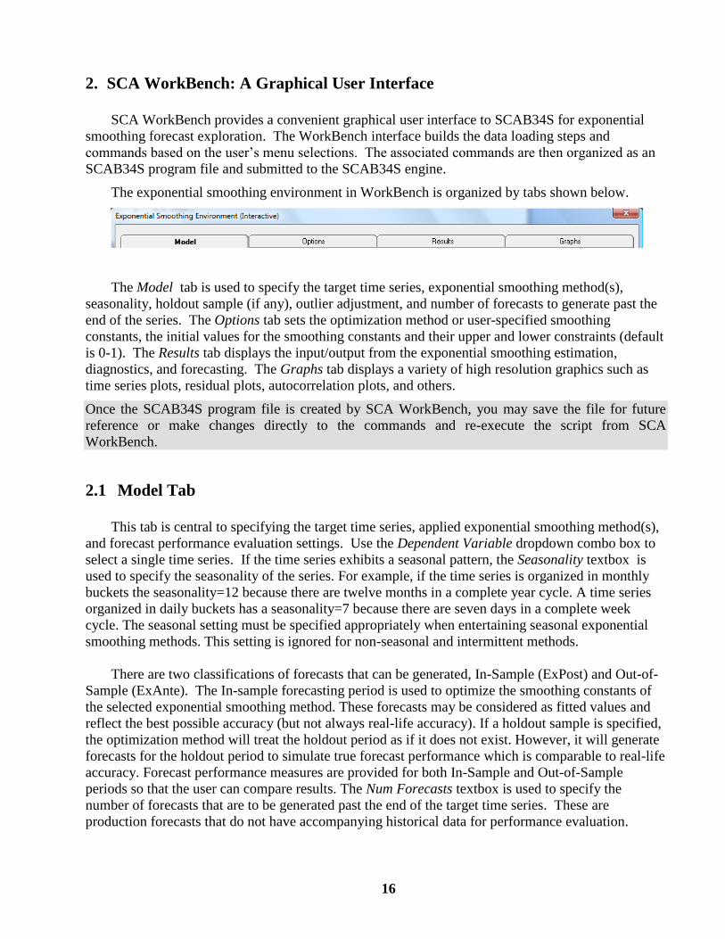
The exponential smoothing environment in WorkBench is organized by tabs shown below.
The Model tab is used to specify the target time series, exponential smoothing method(s),
seasonality, holdout sample (if any), outlier adjustment, and number of forecasts to generate past the
end of the series. The Options tab sets the optimization method or user-specified smoothing
constants, the initial values for the smoothing constants and their upper and lower constraints (default
is 0-1). The Results tab displays the input/output from the exponential smoothing estimation,
diagnostics, and forecasting. The Graphs tab displays a variety of high resolution graphics such as
time series plots, residual plots, autocorrelation plots, and others.
Once the SCAB34S program file is created by SCA WorkBench, you may save the file for future
reference or make changes directly to the commands and re-execute the script from SCA
WorkBench.
2.1 Model Tab
This tab is central to specifying the target time series, applied exponential smoothing method(s),
and forecast performance evaluation settings. Use the Dependent Variable dropdown combo box to
select a single time series. If the time series exhibits a seasonal pattern, the Seasonality textbox is
used to specify the seasonality of the series. For example, if the time series is organized in monthly
buckets the seasonality=12 because there are twelve months in a complete year cycle. A time series
organized in daily buckets has a seasonality=7 because there are seven days in a complete week
cycle. The seasonal setting must be specified appropriately when entertaining seasonal exponential
smoothing methods. This setting is ignored for non-seasonal and intermittent methods.
There are two classifications of forecasts that can be generated, In-Sample (ExPost) and Out-of-
Sample (ExAnte). The In-sample forecasting period is used to optimize the smoothing constants of
the selected exponential smoothing method. These forecasts may be considered as fitted values and
reflect the best possible accuracy (but not always real-life accuracy). If a holdout sample is specified,
the optimization method will treat the holdout period as if it does not exist. However, it will generate
forecasts for the holdout period to simulate true forecast performance which is comparable to real-life
accuracy. Forecast performance measures are provided for both In-Sample and Out-of-Sample
periods so that the user can compare results. The Num Forecasts textbox is used to specify the
number of forecasts that are to be generated past the end of the target time series. These are
production forecasts that do not have accompanying historical data for performance evaluation.
17
A primary goal of forecasting is to leverage the consistent and stable historical patterns in a time
series and extrapolate those patterns into useable predictions for the future. That said, it is important
to eliminate the effect of outliers in model identification, estimation, and forecasting. The user can
select the Enable outlier adjustment checkbox to evaluate the effect of identified outliers on
forecasting performance and on the selection of exponential smoothing methods. The Z-Crit Value
textbox is used to set the threshold for outlier detection. It is recommended that the Z-Crit Value be
set between 2.5 and 5.0 in practice. If the threshold is set too low, a large number of false positive
outlier classifications may occur. Too high of a setting will mask the effect of an outlier.
The Model tab allows the user to select from nineteen forecasting methods. The methods are
grouped as non-seasonal, additive seasonal, multiplicative seasonal, and intermittent. The user can
specify a single forecasting method or multiple forecasting methods to apply to the target time series.
Multiple methods are evaluated by selecting the Determine best from selected methods checkbox and
then selecting the methods of interest. A checkbox is also provided next to the model groups to allow
the user to select or unselect a group of methods. The more methods selected, the more time it will
take to complete the analysis. When the task is completed, the methods will be ranked by accuracy.
The ranking method used is dependent on whether outlier adjustment is enabled and whether a
holdout sample is specified. Ranking is based on a scaled mean absolute deviation (Scaled MAD)
performance measure which is suitable for both continuous and intermittent time series,
n
t tt 1ˆY Y
nsMADY
When outlier adjustment is disabled, ranking is based on the Scaled MAD for the original series
with no outliers removed. When outlier adjustment is enabled, the method selection is based on a
weighted rank that combines the Scaled MAD for a) original series with no outliers removed, and b)
adjusted series with outliers removed. The weighted method is used to safeguard against the
possibility of too many observations being removed as outliers. Furthermore, if a holdout sample is
not specified, the Scaled MAD in the In-Sample (ExPost) period is used. If a holdout sample is
specified, both the In-Sample (ExPost) and the Out-of-Sample (ExAnte) periods are used (scaled by
the number of cases). If the user wishes to use alternative ranking methods, the script may be
modified by the user.
18
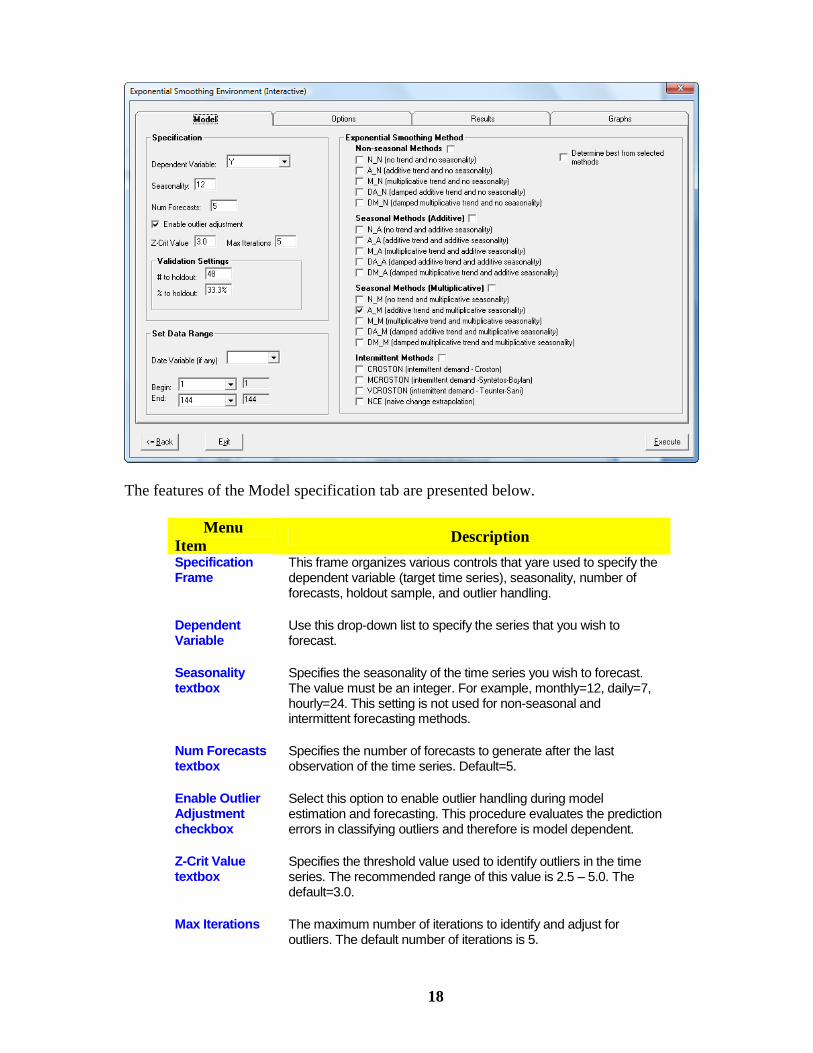
The features of the Model specification tab are presented below.
Menu
Item Description
Specification Frame
This frame organizes various controls that yare used to specify the dependent variable (target time series), seasonality, number of forecasts, holdout sample, and outlier handling.
Dependent Variable
Use this drop-down list to specify the series that you wish to forecast.
Seasonality textbox
Specifies the seasonality of the time series you wish to forecast. The value must be an integer. For example, monthly=12, daily=7, hourly=24. This setting is not used for non-seasonal and intermittent forecasting methods.
Num Forecasts textbox
Specifies the number of forecasts to generate after the last observation of the time series. Default=5.
Enable Outlier Adjustment checkbox
Select this option to enable outlier handling during model estimation and forecasting. This procedure evaluates the prediction errors in classifying outliers and therefore is model dependent.
Z-Crit Value textbox
Specifies the threshold value used to identify outliers in the time series. The recommended range of this value is 2.5 – 5.0. The default=3.0.
Max Iterations The maximum number of iterations to identify and adjust for outliers. The default number of iterations is 5.

19
# to Holdout Specifies the number of observations at the end of the time series to holdout for Out-Of-Sample (ExAnte) forecast performance.
Exponential Smoothing Method Frame
Select among 19 various exponential smoothing methods to perform forecasting and performance evaluation. Methods cover non-seasonal, additive seasonal, multiplicative seasonal, and intermittent classes of time series
Determine Best From Selected Methods checkbox
Select his option to evaluate more than one selected exponential smoothing method and compare their relative forecasting performance
Set Data Range Frame
This frame organizes form controls related to how the data is indexed (by date or none), and what data span is modeled and analyzed.
Date Variable Use this drop-down list to specify the date variable associated with your series. If your SCA Data Macro contains a variable named "DATE", it is automatically assigned by SCA WorkBench. If you have an alternative index variable or date variable, you may select it from the drop-down list. If your SCA Data Macro does not contain a DATE variable, leave the dropdown list empty. WorkBench will then use the observation number as a date index. If your time series is more than 10,000 observations, WorkBench will not use your DATE variable for indexing. Instead, observation number will be used.
Begin Span Use the Begin drop-down list to omit observations from the beginning of a time series being analyzed.
End Span Use the End drop-down list to omit observations from the back of a time series being analyzed.
Back Depending on the tab you are currently working in, clicking on the Back button will move you one tab to the left. If you are in the Model tab, you will move to the Exponential Smoothing Data Viewer dialog box where you may choose a new SCA data macro or leave the Exponential Smoothing Forecasting environment.
Exit Exits the Exponential Smoothing Forecasting environment.
Execute Executes exponential smoothing optimization, validation, performance comparison, diagnostics, and graphs by submitting a dynamically created program script to SCAB34S. When completed, you will automatically be placed in the Results tab.
20
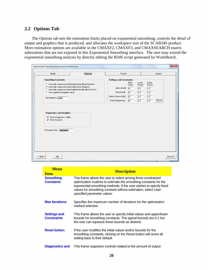
2.2 Options Tab
The Options tab sets the estimation limits placed on exponential smoothing, controls the detail of
output and graphics that is produced, and allocates the workspace size of the SCAB34S product.
More estimation options are available in the CMAXF2, CMAXF3, and CMAXSEARCH matrix
subroutines that are not exposed in this Exponential Smoothing interface. The user may extend the
exponential smoothing analysis by directly editing the B34S script generated by WorkBench.
Menu
Item Description
Smoothing Constants
This frame allows the user to select among three constrained optimization routines to estimate the smoothing constants for the exponential smoothing methods. If the user wishes to specify fixed values for smoothing constant without estimation, select User specified parameter values
Max Iterations Specifies the maximum number of iterations for the optimization method selected.
Settings and Constraints
This frame allows the user to specify initial values and upper/lower bounds for smoothing constants. The typical bounds are 0-1 but the user can squeeze these bounds as desired.
Reset button If the user modifies the initial values and/or bounds for the smoothing constants, clicking on the Reset button will revert all setting back to their default.
Diagnostics and This frame organizes controls related to the amount of output

21
Graphics Frame produced for exponential smoothing forecasting and diagnostics.
Display Output for Model
Typically, you want to see the model summary.
Show Diagnostic Tables
Several diagnostics are available for the dependent variable and the residuals from the estimated models.
Show Graphics Several graphics are created including time plot of the dependent variable, Actual vs. Predicted, Forecast, ACF and PACF plots, and modified Q-Statistic plot.
Workspace Size The SCAB34S product requires its workspace size to be set when the program is initiated. The default workspace is of 2000000 is adequate to handle moderate size datasets. The user may increase the workspace size if needed. Please note that workspace limit is imposed by the amount of available RAM memory of the computer.
22
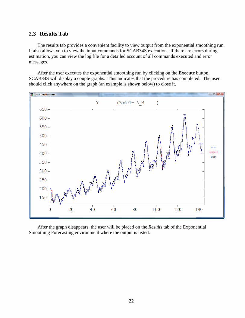
2.3 Results Tab
The results tab provides a convenient facility to view output from the exponential smoothing run.
It also allows you to view the input commands for SCAB34S execution. If there are errors during
estimation, you can view the log file for a detailed account of all commands executed and error
messages.
After the user executes the exponential smoothing run by clicking on the Execute button,
SCAB34S will display a couple graphs. This indicates that the procedure has completed. The user
should click anywhere on the graph (an example is shown below) to close it.
After the graph disappears, the user will be placed on the Results tab of the Exponential
Smoothing Forecasting environment where the output is listed.
23
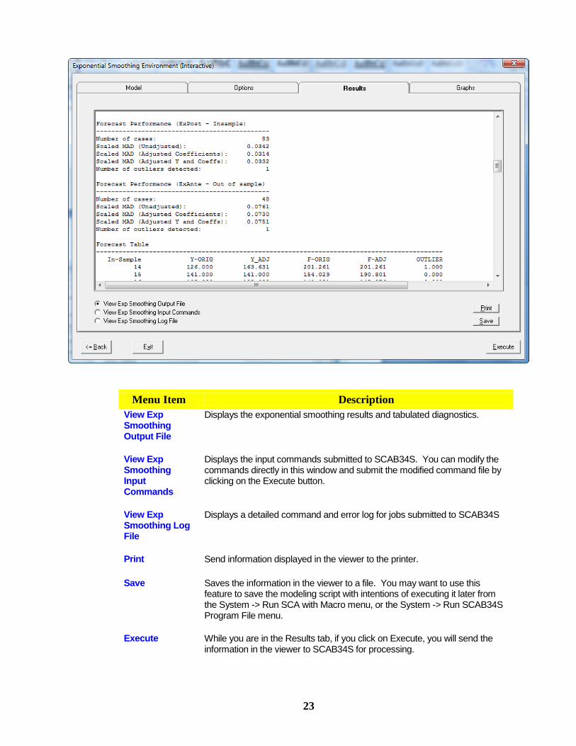
Menu Item Description
View Exp Smoothing Output File
Displays the exponential smoothing results and tabulated diagnostics.
View Exp Smoothing Input Commands
Displays the input commands submitted to SCAB34S. You can modify the commands directly in this window and submit the modified command file by clicking on the Execute button.
View Exp Smoothing Log File
Displays a detailed command and error log for jobs submitted to SCAB34S
Print Send information displayed in the viewer to the printer.
Save Saves the information in the viewer to a file. You may want to use this feature to save the modeling script with intentions of executing it later from the System -> Run SCA with Macro menu, or the System -> Run SCAB34S Program File menu.
Execute While you are in the Results tab, if you click on Execute, you will send the information in the viewer to SCAB34S for processing.
24
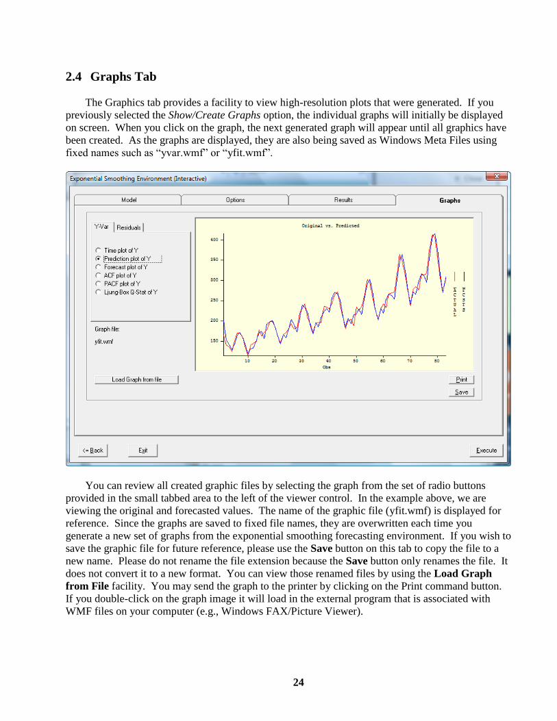
2.4 Graphs Tab
The Graphics tab provides a facility to view high-resolution plots that were generated. If you
previously selected the Show/Create Graphs option, the individual graphs will initially be displayed
on screen. When you click on the graph, the next generated graph will appear until all graphics have
been created. As the graphs are displayed, they are also being saved as Windows Meta Files using
fixed names such as “yvar.wmf” or “yfit.wmf”.
You can review all created graphic files by selecting the graph from the set of radio buttons
provided in the small tabbed area to the left of the viewer control. In the example above, we are
viewing the original and forecasted values. The name of the graphic file (yfit.wmf) is displayed for
reference. Since the graphs are saved to fixed file names, they are overwritten each time you
generate a new set of graphs from the exponential smoothing forecasting environment. If you wish to
save the graphic file for future reference, please use the Save button on this tab to copy the file to a
new name. Please do not rename the file extension because the Save button only renames the file. It
does not convert it to a new format. You can view those renamed files by using the Load Graph
from File facility. You may send the graph to the printer by clicking on the Print command button.
If you double-click on the graph image it will load in the external program that is associated with
WMF files on your computer (e.g., Windows FAX/Picture Viewer).
25
3. EXAMPLES OF EXPONENTIAL SMOOTHING USING SCA
WORKBENCH
This section provides a few exponential smoothing examples using SCA WorkBench and its
interface to SCAB34S. The first example uses Pegels’ exponential smoothing with multivariate trend
to forecast monthly inventory of durable goods. In the second example, we will automatically
identify an appropriate seasonal exponential smoothing method for monthly airline passenger load.
The third example explores intermittent demand forecasting using the Croston method and its
modifications.
The data files used for the examples discussed in this section are available under the WorkBench
installation folder in a sub-directory named TSDATA. The command files built by SCA WorkBench
for the illustrated examples are presented later in Section 0 of this document.
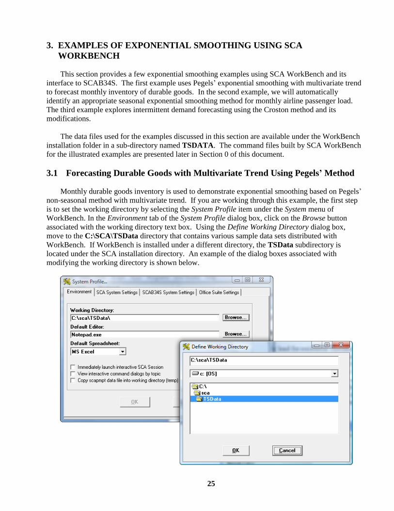
3.1 Forecasting Durable Goods with Multivariate Trend Using Pegels’ Method
Monthly durable goods inventory is used to demonstrate exponential smoothing based on Pegels’
non-seasonal method with multivariate trend. If you are working through this example, the first step
is to set the working directory by selecting the System Profile item under the System menu of
WorkBench. In the Environment tab of the System Profile dialog box, click on the Browse button
associated with the working directory text box. Using the Define Working Directory dialog box,
move to the C:\SCA\TSData directory that contains various sample data sets distributed with
WorkBench. If WorkBench is installed under a different directory, the TSData subdirectory is
located under the SCA installation directory. An example of the dialog boxes associated with
modifying the working directory is shown below.
26
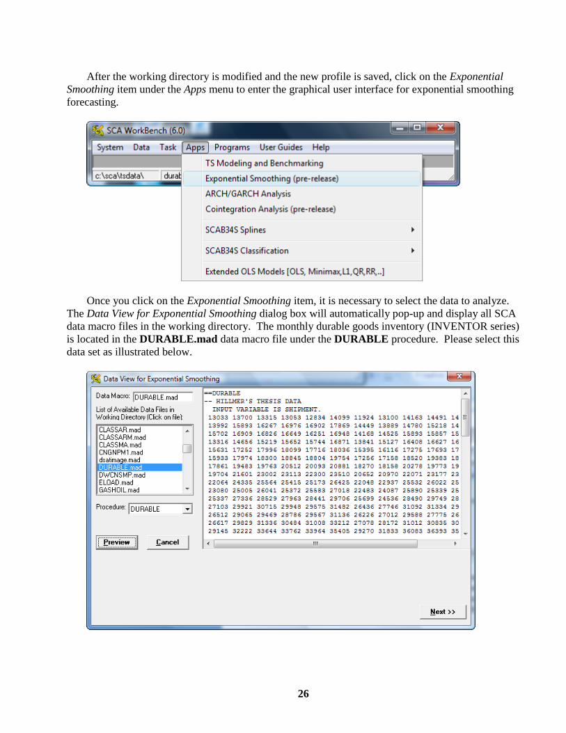
After the working directory is modified and the new profile is saved, click on the Exponential
Smoothing item under the Apps menu to enter the graphical user interface for exponential smoothing
forecasting.
Once you click on the Exponential Smoothing item, it is necessary to select the data to analyze.
The Data View for Exponential Smoothing dialog box will automatically pop-up and display all SCA
data macro files in the working directory. The monthly durable goods inventory (INVENTOR series)
is located in the DURABLE.mad data macro file under the DURABLE procedure. Please select this
data set as illustrated below.
27
The data may be viewed by clicking on the Preview button. The DURABLE data set consists of
three series although we will only use INVENTOR here:
SHIPMENT Durable goods monthly shipments
NEWORDER New orders for durable goods
INVENTORY Monthly inventory of durable goods
In this example, we specify the M_N (multivariate trend – no seasonality) for the INVENTOR
time series. Click on the Next button to enter the Exponential Smoothing Environment.
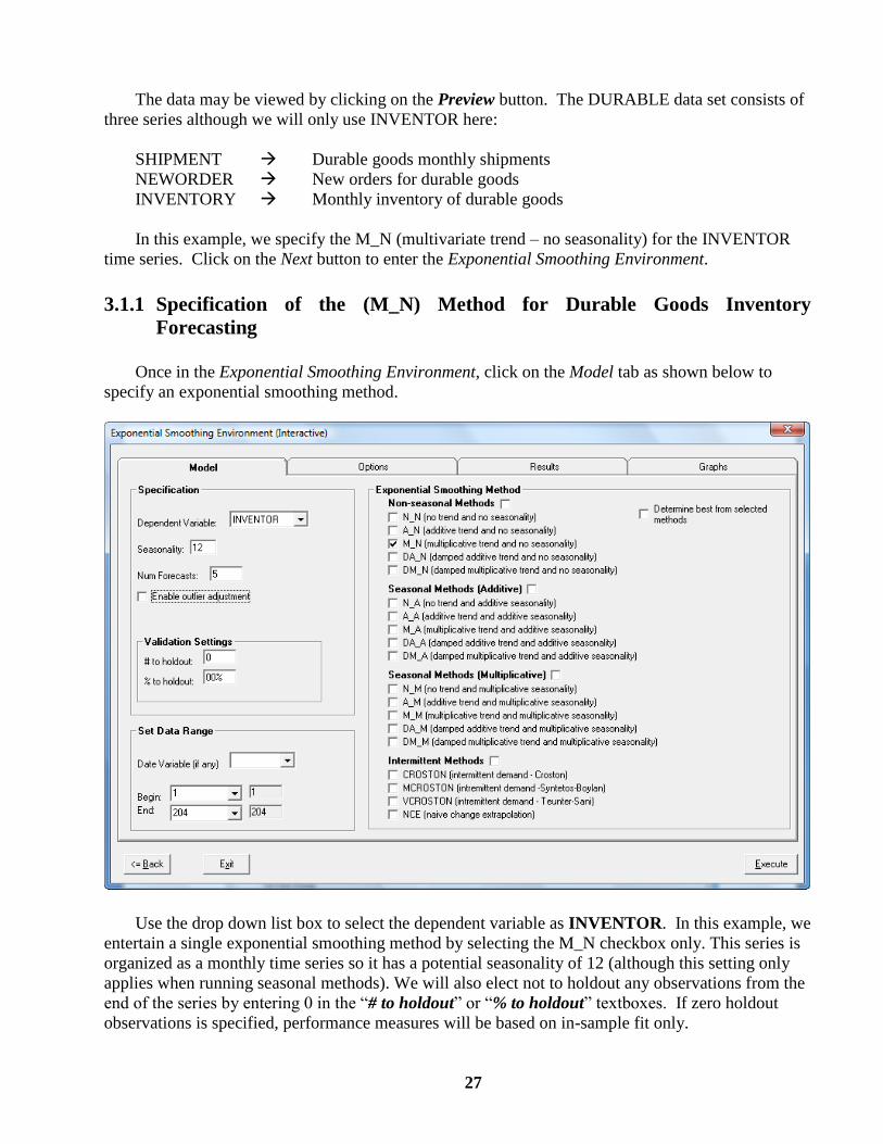
3.1.1 Specification of the (M_N) Method for Durable Goods Inventory
Forecasting
Once in the Exponential Smoothing Environment, click on the Model tab as shown below to
specify an exponential smoothing method.
Use the drop down list box to select the dependent variable as INVENTOR. In this example, we
entertain a single exponential smoothing method by selecting the M_N checkbox only. This series is
organized as a monthly time series so it has a potential seasonality of 12 (although this setting only
applies when running seasonal methods). We will also elect not to holdout any observations from the
end of the series by entering 0 in the “# to holdout” or “% to holdout” textboxes. If zero holdout
observations is specified, performance measures will be based on in-sample fit only.
28
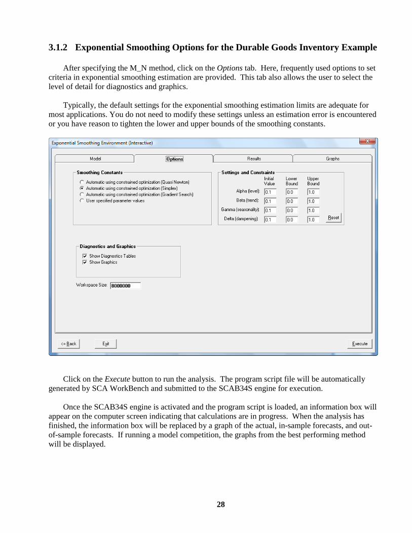
3.1.2 Exponential Smoothing Options for the Durable Goods Inventory Example
After specifying the M_N method, click on the Options tab. Here, frequently used options to set
criteria in exponential smoothing estimation are provided. This tab also allows the user to select the
level of detail for diagnostics and graphics.
Typically, the default settings for the exponential smoothing estimation limits are adequate for
most applications. You do not need to modify these settings unless an estimation error is encountered
or you have reason to tighten the lower and upper bounds of the smoothing constants.
Click on the Execute button to run the analysis. The program script file will be automatically
generated by SCA WorkBench and submitted to the SCAB34S engine for execution.
Once the SCAB34S engine is activated and the program script is loaded, an information box will
appear on the computer screen indicating that calculations are in progress. When the analysis has
finished, the information box will be replaced by a graph of the actual, in-sample forecasts, and out-
of-sample forecasts. If running a model competition, the graphs from the best performing method
will be displayed.
29
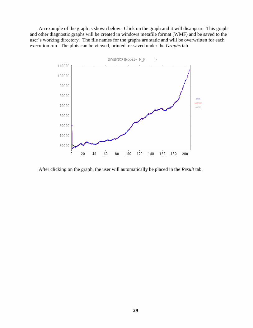
An example of the graph is shown below. Click on the graph and it will disappear. This graph
and other diagnostic graphs will be created in windows metafile format (WMF) and be saved to the
user’s working directory. The file names for the graphs are static and will be overwritten for each
execution run. The plots can be viewed, printed, or saved under the Graphs tab.
INVENTOR(Model= M_N )
0 20 40 60 80 100 120 140 160 180 2000 20 40 60 80 100 120 140 160 180 200
30000
40000
50000
60000
70000
80000
90000
100000
110000
0 20 40 60 80 100 120 140 160 180 200
ORIGY
ADJFCST
FCST
After clicking on the graph, the user will automatically be placed in the Result tab.
30
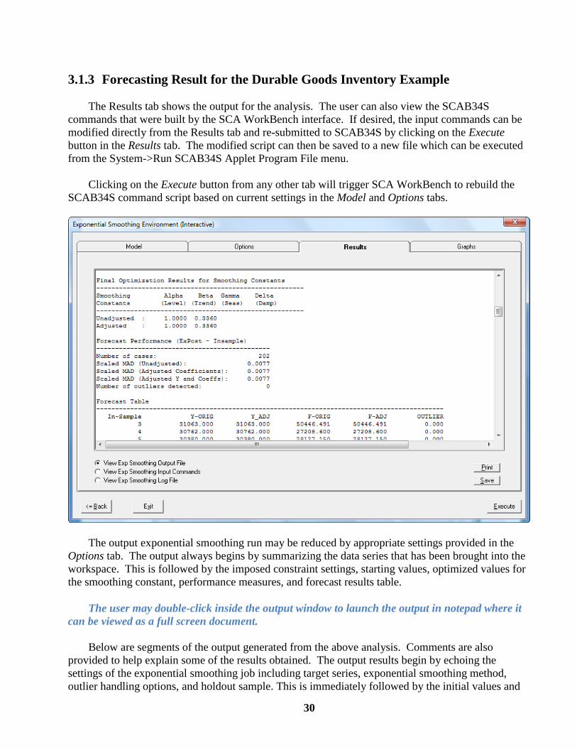
3.1.3 Forecasting Result for the Durable Goods Inventory Example
The Results tab shows the output for the analysis. The user can also view the SCAB34S
commands that were built by the SCA WorkBench interface. If desired, the input commands can be
modified directly from the Results tab and re-submitted to SCAB34S by clicking on the Execute
button in the Results tab. The modified script can then be saved to a new file which can be executed
from the System->Run SCAB34S Applet Program File menu.
Clicking on the Execute button from any other tab will trigger SCA WorkBench to rebuild the
SCAB34S command script based on current settings in the Model and Options tabs.
The output exponential smoothing run may be reduced by appropriate settings provided in the
Options tab. The output always begins by summarizing the data series that has been brought into the
workspace. This is followed by the imposed constraint settings, starting values, optimized values for
the smoothing constant, performance measures, and forecast results table.
The user may double-click inside the output window to launch the output in notepad where it
can be viewed as a full screen document.
Below are segments of the output generated from the above analysis. Comments are also
provided to help explain some of the results obtained. The output results begin by echoing the
settings of the exponential smoothing job including target series, exponential smoothing method,
outlier handling options, and holdout sample. This is immediately followed by the initial values and
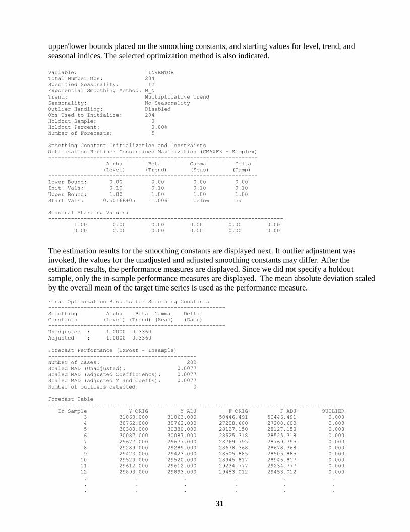
31
upper/lower bounds placed on the smoothing constants, and starting values for level, trend, and
seasonal indices. The selected optimization method is also indicated.
Variable: INVENTOR
Total Number Obs: 204
Specified Seasonality: 12
Exponential Smoothing Method: M_N
Trend: Multiplicative Trend
Seasonality: No Seasonality
Outlier Handling: Disabled
Obs Used to Initialize: 204
Holdout Sample: 0
Holdout Percent: 0.00%
Number of Forecasts: 5
Smoothing Constant Initialization and Constraints
Optimization Routine: Constrained Maximization (CMAXF3 - Simplex)
-----------------------------------------------------------------
Alpha Beta Gamma Delta
(Level) (Trend) (Seas) (Damp)
-----------------------------------------------------------------
Lower Bound: 0.00 0.00 0.00 0.00
Init. Vals: 0.10 0.10 0.10 0.10
Upper Bound: 1.00 1.00 1.00 1.00
Start Vals: 0.5016E+05 1.006 below na
Seasonal Starting Values:
-------------------------------------------------------------------------
1.00 0.00 0.00 0.00 0.00 0.00
0.00 0.00 0.00 0.00 0.00 0.00
The estimation results for the smoothing constants are displayed next. If outlier adjustment was
invoked, the values for the unadjusted and adjusted smoothing constants may differ. After the
estimation results, the performance measures are displayed. Since we did not specify a holdout
sample, only the in-sample performance measures are displayed. The mean absolute deviation scaled
by the overall mean of the target time series is used as the performance measure.
Final Optimization Results for Smoothing Constants
-------------------------------------------------------
Smoothing Alpha Beta Gamma Delta
Constants (Level) (Trend) (Seas) (Damp)
-------------------------------------------------------
Unadjusted : 1.0000 0.3360
Adjusted : 1.0000 0.3360
Forecast Performance (ExPost - Insample)
----------------------------------------------
Number of cases: 202
Scaled MAD (Unadjusted): 0.0077
Scaled MAD (Adjusted Coefficients): 0.0077
Scaled MAD (Adjusted Y and Coeffs): 0.0077
Number of outliers detected: 0
Forecast Table
--------------------------------------------------------------------------------------------
In-Sample Y-ORIG Y_ADJ F-ORIG F-ADJ OUTLIER
3 31063.000 31063.000 50446.491 50446.491 0.000
4 30762.000 30762.000 27208.600 27208.600 0.000
5 30380.000 30380.000 28127.150 28127.150 0.000
6 30087.000 30087.000 28525.318 28525.318 0.000
7 29677.000 29677.000 28769.795 28769.795 0.000
8 29289.000 29289.000 28678.368 28678.368 0.000
9 29423.000 29423.000 28505.885 28505.885 0.000
10 29520.000 29520.000 28945.817 28945.817 0.000
11 29612.000 29612.000 29234.777 29234.777 0.000
12 29893.000 29893.000 29453.012 29453.012 0.000
. . . . . .
. . . . . .
. . . . . .
32
Forecast -----------------------------------------------------------------------------------
205 98906.229 98906.229
206 100644.479 100644.479
207 102413.278 102413.278
208 104213.164 104213.164
209 106044.682 106044.682
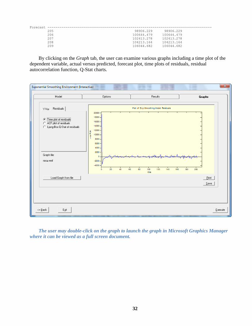
By clicking on the Graph tab, the user can examine various graphs including a time plot of the
dependent variable, actual versus predicted, forecast plot, time plots of residuals, residual
autocorrelation function, Q-Stat charts.
The user may double-click on the graph to launch the graph in Microsoft Graphics Manager
where it can be viewed as a full screen document.
33
3.2 Forecasting Seasonal Airline Passenger Load Based on Automatic Method
Selection
Monthly airline passenger load is used to demonstrate automatic selection of an exponential
smoothing method for forecasting. If you are working through this example, the first step is to set the
working directory by selecting the System Profile item under the System menu of WorkBench. In the
Environment tab of the System Profile dialog box, click on the Browse button associated with the
working directory text box. Using the Define Working Directory dialog box, move to the
C:\SCA\TSData directory that contains various sample data sets distributed with WorkBench. If
WorkBench is installed under a different directory, the TSData subdirectory is located under the
SCA installation directory.
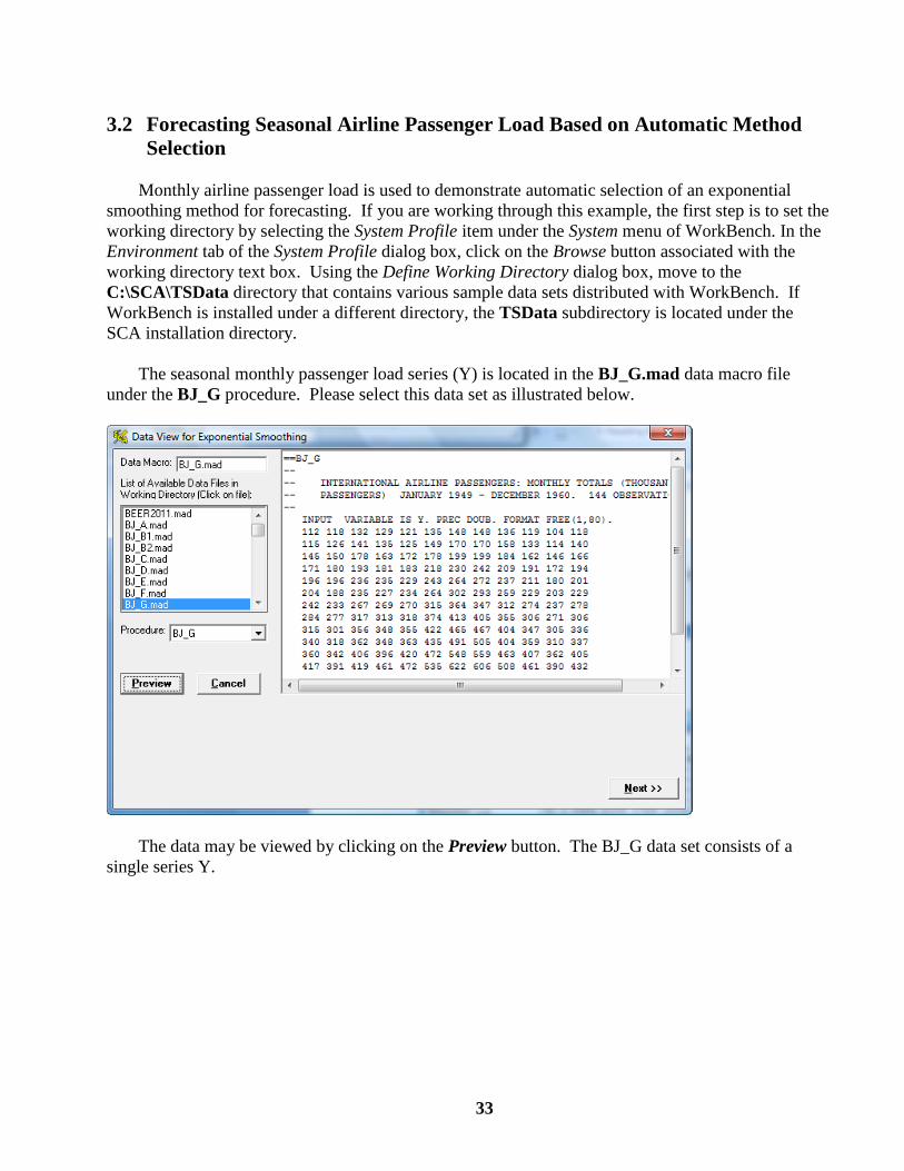
The seasonal monthly passenger load series (Y) is located in the BJ_G.mad data macro file
under the BJ_G procedure. Please select this data set as illustrated below.
The data may be viewed by clicking on the Preview button. The BJ_G data set consists of a
single series Y.
34
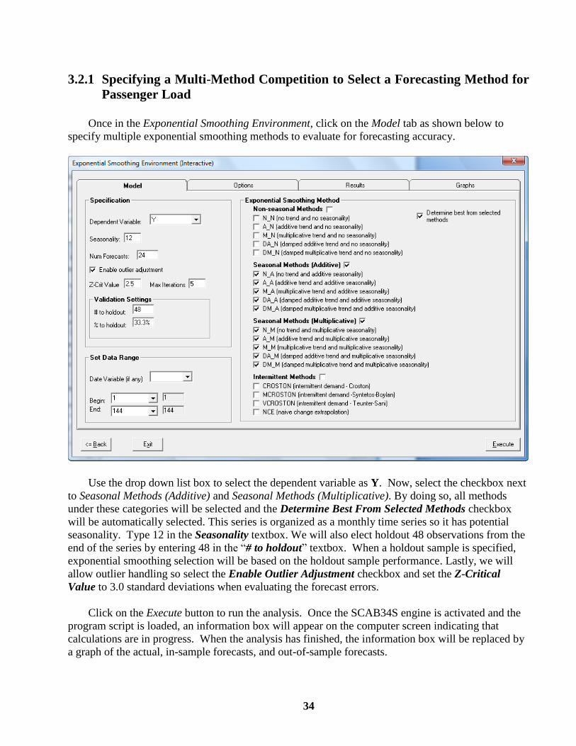
3.2.1 Specifying a Multi-Method Competition to Select a Forecasting Method for
Passenger Load
Once in the Exponential Smoothing Environment, click on the Model tab as shown below to
specify multiple exponential smoothing methods to evaluate for forecasting accuracy.
Use the drop down list box to select the dependent variable as Y. Now, select the checkbox next
to Seasonal Methods (Additive) and Seasonal Methods (Multiplicative). By doing so, all methods
under these categories will be selected and the Determine Best From Selected Methods checkbox
will be automatically selected. This series is organized as a monthly time series so it has potential
seasonality. Type 12 in the Seasonality textbox. We will also elect holdout 48 observations from the
end of the series by entering 48 in the “# to holdout” textbox. When a holdout sample is specified,
exponential smoothing selection will be based on the holdout sample performance. Lastly, we will
allow outlier handling so select the Enable Outlier Adjustment checkbox and set the Z-Critical
Value to 3.0 standard deviations when evaluating the forecast errors.
Click on the Execute button to run the analysis. Once the SCAB34S engine is activated and the
program script is loaded, an information box will appear on the computer screen indicating that
calculations are in progress. When the analysis has finished, the information box will be replaced by
a graph of the actual, in-sample forecasts, and out-of-sample forecasts.
35
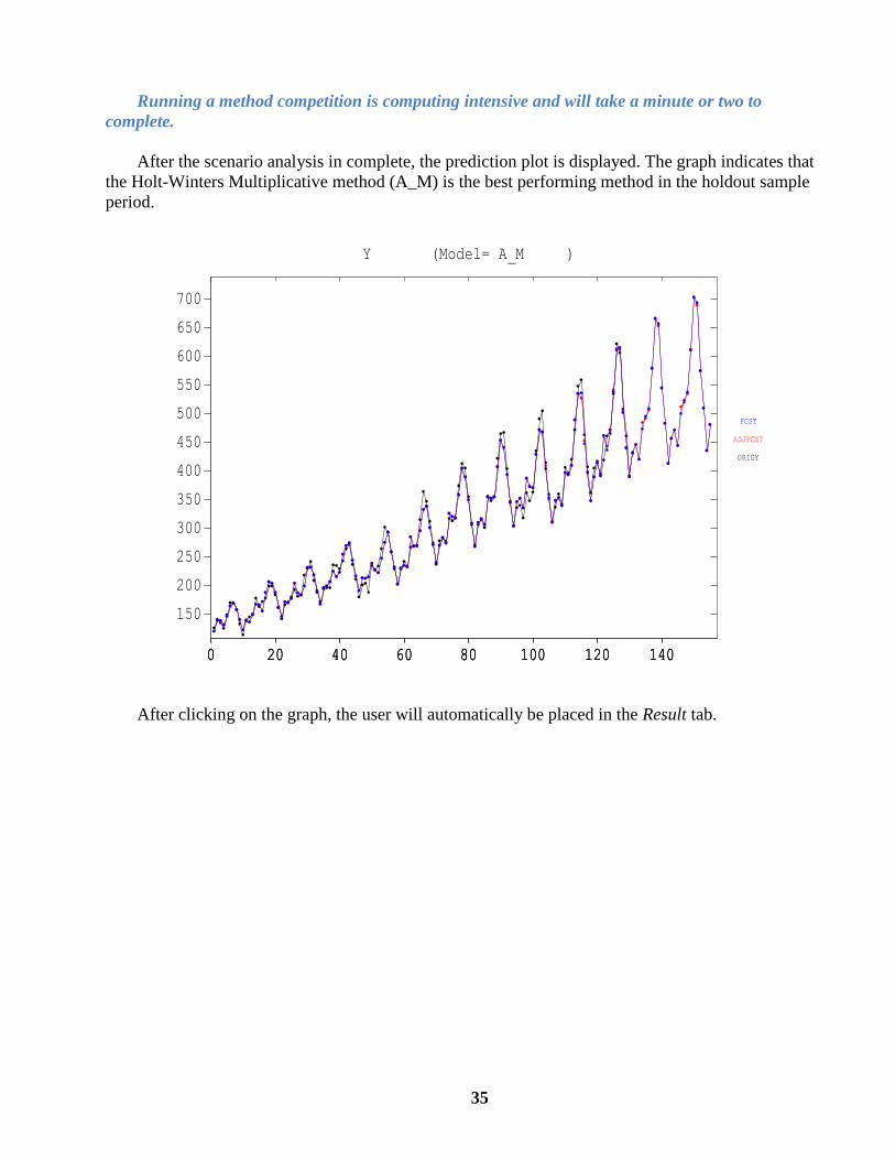
Running a method competition is computing intensive and will take a minute or two to
complete.
After the scenario analysis in complete, the prediction plot is displayed. The graph indicates that
the Holt-Winters Multiplicative method (A_M) is the best performing method in the holdout sample
period.
Y (Model= A_M )
0 20 40 60 80 100 120 1400 20 40 60 80 100 120 140
150
200
250
300
350
400
450
500
550
600
650
700
0 20 40 60 80 100 120 140
ORIGY
ADJFCST
FCST
After clicking on the graph, the user will automatically be placed in the Result tab.
36
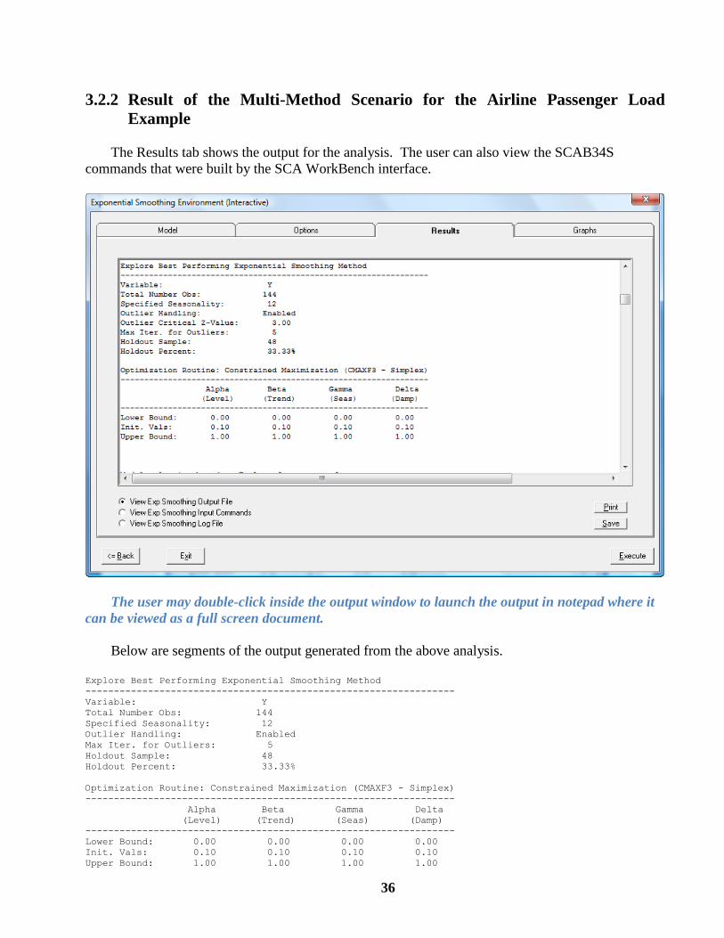
3.2.2 Result of the Multi-Method Scenario for the Airline Passenger Load
Example
The Results tab shows the output for the analysis. The user can also view the SCAB34S
commands that were built by the SCA WorkBench interface.
The user may double-click inside the output window to launch the output in notepad where it
can be viewed as a full screen document.
Below are segments of the output generated from the above analysis.
Explore Best Performing Exponential Smoothing Method
-----------------------------------------------------------------
Variable: Y
Total Number Obs: 144
Specified Seasonality: 12
Outlier Handling: Enabled
Max Iter. for Outliers: 5
Holdout Sample: 48
Holdout Percent: 33.33%
Optimization Routine: Constrained Maximization (CMAXF3 - Simplex)
-----------------------------------------------------------------
Alpha Beta Gamma Delta
(Level) (Trend) (Seas) (Damp)
-----------------------------------------------------------------
Lower Bound: 0.00 0.00 0.00 0.00
Init. Vals: 0.10 0.10 0.10 0.10
Upper Bound: 1.00 1.00 1.00 1.00
37
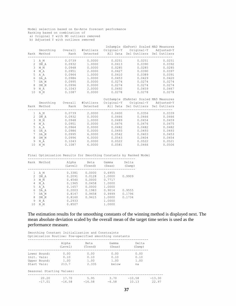
Model selection based on Ex-Ante forecast performance
Ranking based on combination of
a) Original Y with NO outliers removed
b) Adjusted Y with outliers removed
InSample (ExPost) Scaled MAD Measures
Smoothing Overall #Outliers Original-Y Original-Y Adjusted-Y
Rank Method Rank Detected All Data Del Outliers Del Outliers
------------------------------------------------------------------------------
1 A_M 0.0739 0.0000 0.0251 0.0251 0.0251
2 DM_A 0.0932 1.0000 0.0413 0.0390 0.0392
3 M_M 0.0948 0.0000 0.0285 0.0285 0.0285
4 M_A 0.0951 2.0000 0.0427 0.0390 0.0397
5 A_A 0.0964 1.0000 0.0410 0.0389 0.0391
6 DA_A 0.0986 1.0000 0.0453 0.0429 0.0420
7 DA_M 0.0995 0.0000 0.0274 0.0274 0.0274
8 DM_M 0.0996 0.0000 0.0274 0.0274 0.0274
9 N_A 0.1043 2.0000 0.0492 0.0459 0.0467
10 N_M 0.1087 0.0000 0.0278 0.0278 0.0278
OutSample (ExAnte) Scaled MAD Measures
Smoothing Overall #Outliers Original-Y Original-Y Adjusted-Y
Rank Method Rank Detected All Data Del Outliers Del Outliers
------------------------------------------------------------------------------
1 A_M 0.0739 2.0000 0.0400 0.0356 0.0339
2 DM_A 0.0932 0.0000 0.0466 0.0466 0.0466
3 M_M 0.0948 1.0000 0.0489 0.0454 0.0459
4 M_A 0.0951 0.0000 0.0476 0.0476 0.0475
5 A_A 0.0964 0.0000 0.0482 0.0482 0.0482
6 DA_A 0.0986 0.0000 0.0493 0.0493 0.0493
7 DA_M 0.0995 6.0000 0.0542 0.0403 0.0453
8 DM_M 0.0996 6.0000 0.0543 0.0404 0.0454
9 N_A 0.1043 0.0000 0.0522 0.0522 0.0521
10 N_M 0.1087 6.0000 0.0581 0.0466 0.0506
Final Optimization Results for Smoothing Constants by Ranked Model
----------------------------------------------------------
Rank Method Alpha Beta Gamma Delta
(Level) (Trend) (Seas) (Damp)
----------------------------------------------------------
1 A_M 0.3381 0.0000 0.6955
2 DM_A 0.2091 0.0128 1.0000 0.9909
3 M_M 0.4540 0.0000 0.7717
4 M_A 0.1965 0.0458 1.0000
5 A_A 0.1657 0.0000 1.0000
6 DA_A 0.2003 0.1983 0.9014 0.9555
7 DA_M 0.8147 0.9458 0.9999 0.1796
8 DM_M 0.8160 0.9415 1.0000 0.1734
9 N_A 0.2933 1.0000
10 N_M 0.8507 1.0000
The estimation results for the smoothing constants of the winning method is displayed next. The
mean absolute deviation scaled by the overall mean of the target time series is used as the
performance measure.
Smoothing Constant Initialization and Constraints
Optimization Routine: Pre-specified smoothing constants
-----------------------------------------------------------------
Alpha Beta Gamma Delta
(Level) (Trend) (Seas) (Damp)
-----------------------------------------------------------------
Lower Bound: 0.00 0.00 0.00 0.00
Init. Vals: 0.10 0.10 0.10 0.10
Upper Bound: 1.00 1.00 1.00 1.00
Start Vals: 213.7 2.335 below na
Seasonal Starting Values:
-------------------------------------------------------------------------
20.20 17.70 5.95 3.70 -10.58 -13.30
-17.01 -16.58 -16.58 -6.58 10.13 22.97
38
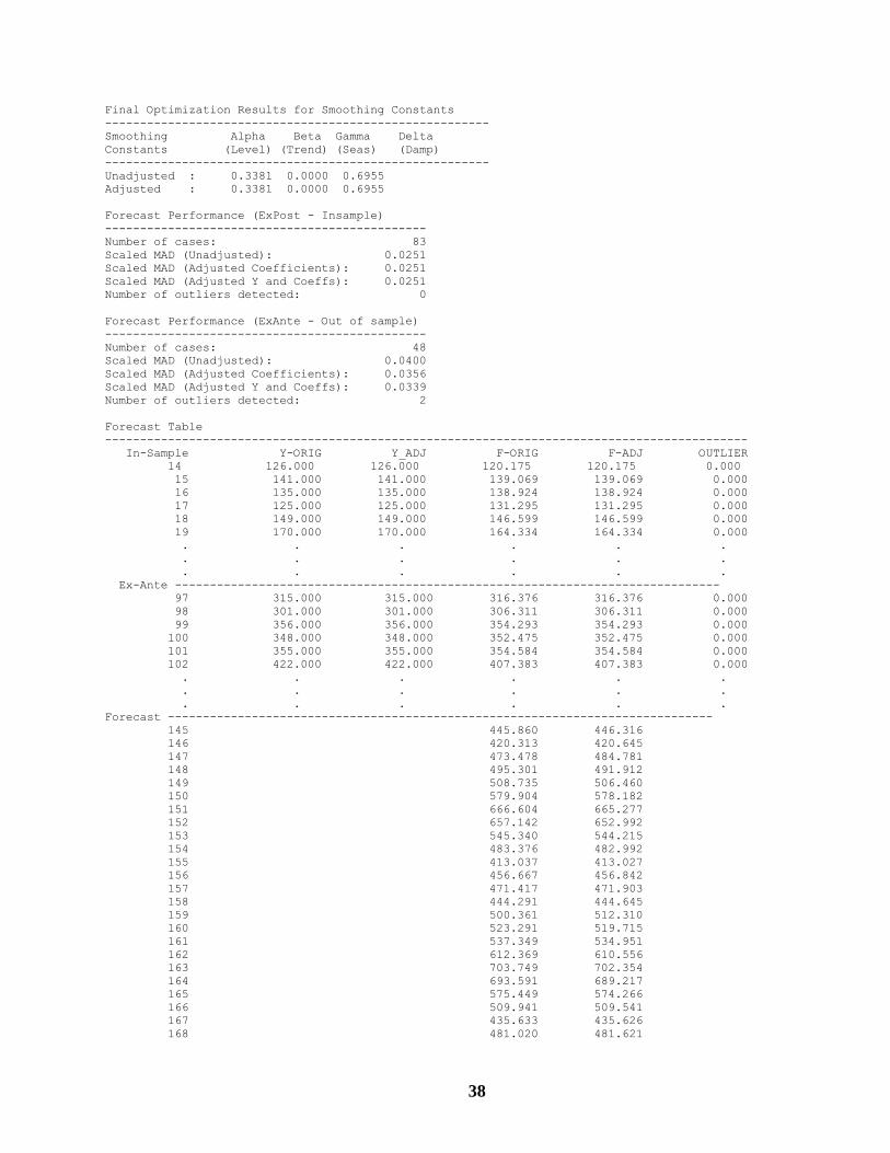
Final Optimization Results for Smoothing Constants
-------------------------------------------------------
Smoothing Alpha Beta Gamma Delta
Constants (Level) (Trend) (Seas) (Damp)
-------------------------------------------------------
Unadjusted : 0.3381 0.0000 0.6955
Adjusted : 0.3381 0.0000 0.6955
Forecast Performance (ExPost - Insample)
----------------------------------------------
Number of cases: 83
Scaled MAD (Unadjusted): 0.0251
Scaled MAD (Adjusted Coefficients): 0.0251
Scaled MAD (Adjusted Y and Coeffs): 0.0251
Number of outliers detected: 0
Forecast Performance (ExAnte - Out of sample)
----------------------------------------------
Number of cases: 48
Scaled MAD (Unadjusted): 0.0400
Scaled MAD (Adjusted Coefficients): 0.0356
Scaled MAD (Adjusted Y and Coeffs): 0.0339
Number of outliers detected: 2
Forecast Table
--------------------------------------------------------------------------------------------
In-Sample Y-ORIG Y_ADJ F-ORIG F-ADJ OUTLIER
14 126.000 126.000 120.175 120.175 0.000
15 141.000 141.000 139.069 139.069 0.000
16 135.000 135.000 138.924 138.924 0.000
17 125.000 125.000 131.295 131.295 0.000
18 149.000 149.000 146.599 146.599 0.000
19 170.000 170.000 164.334 164.334 0.000
. . . . . .
. . . . . .
. . . . . .
Ex-Ante ------------------------------------------------------------------------------
97 315.000 315.000 316.376 316.376 0.000
98 301.000 301.000 306.311 306.311 0.000
99 356.000 356.000 354.293 354.293 0.000
100 348.000 348.000 352.475 352.475 0.000
101 355.000 355.000 354.584 354.584 0.000
102 422.000 422.000 407.383 407.383 0.000
. . . . . .
. . . . . .
. . . . . .
Forecast ------------------------------------------------------------------------------
145 445.860 446.316
146 420.313 420.645
147 473.478 484.781
148 495.301 491.912
149 508.735 506.460
150 579.904 578.182
151 666.604 665.277
152 657.142 652.992
153 545.340 544.215
154 483.376 482.992
155 413.037 413.027
156 456.667 456.842
157 471.417 471.903
158 444.291 444.645
159 500.361 512.310
160 523.291 519.715
161 537.349 534.951
162 612.369 610.556
163 703.749 702.354
164 693.591 689.217
165 575.449 574.266
166 509.941 509.541
167 435.633 435.626
168 481.020 481.621

39
By clicking on the Graph tab, the user can examine various graphs including a time plot of the
dependent variable, actual versus predicted, forecast plot, time plots of residuals, residual
autocorrelation function, Q-Stat charts.
The user may double-click on the graph to launch the graph in Microsoft Graphics Manager
where it can be viewed as a full screen document.
40
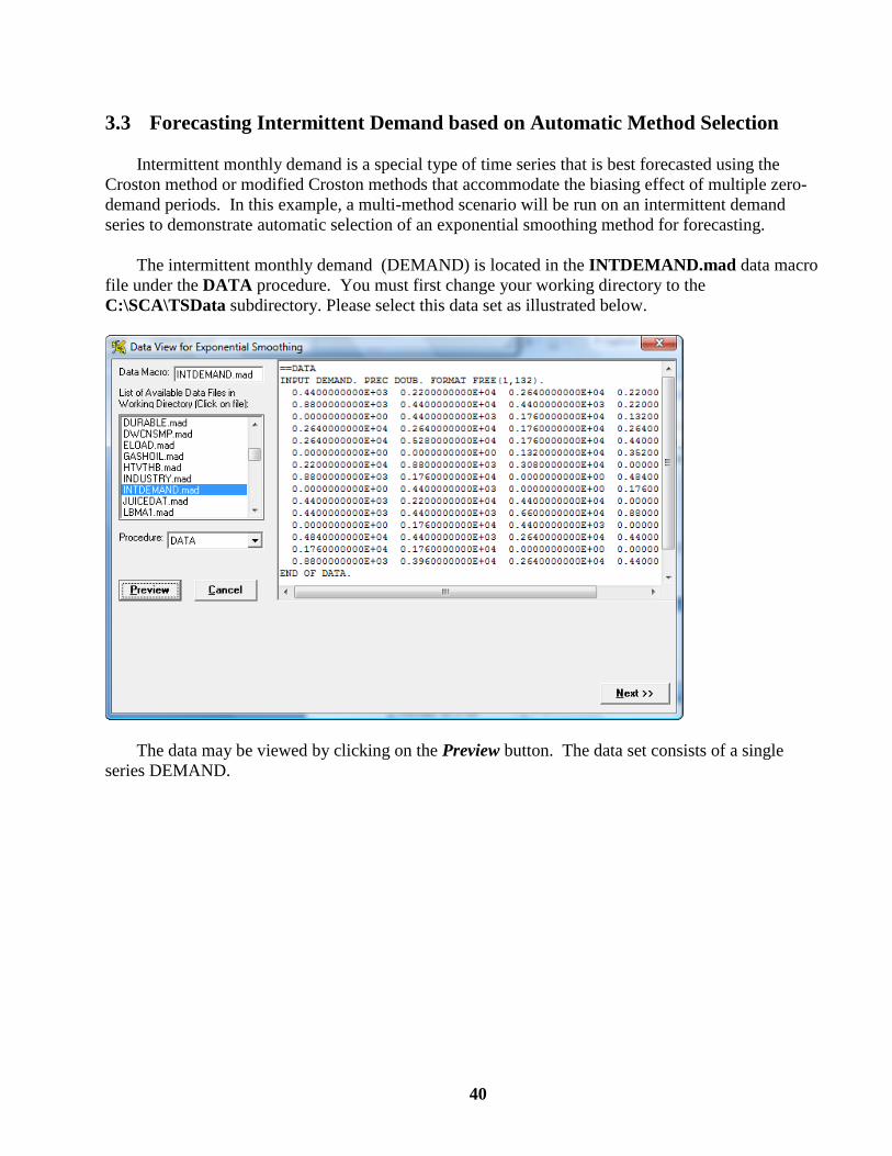
3.3 Forecasting Intermittent Demand based on Automatic Method Selection
Intermittent monthly demand is a special type of time series that is best forecasted using the
Croston method or modified Croston methods that accommodate the biasing effect of multiple zero-
demand periods. In this example, a multi-method scenario will be run on an intermittent demand
series to demonstrate automatic selection of an exponential smoothing method for forecasting.
The intermittent monthly demand (DEMAND) is located in the INTDEMAND.mad data macro
file under the DATA procedure. You must first change your working directory to the
C:\SCA\TSData subdirectory. Please select this data set as illustrated below.
The data may be viewed by clicking on the Preview button. The data set consists of a single
series DEMAND.
41
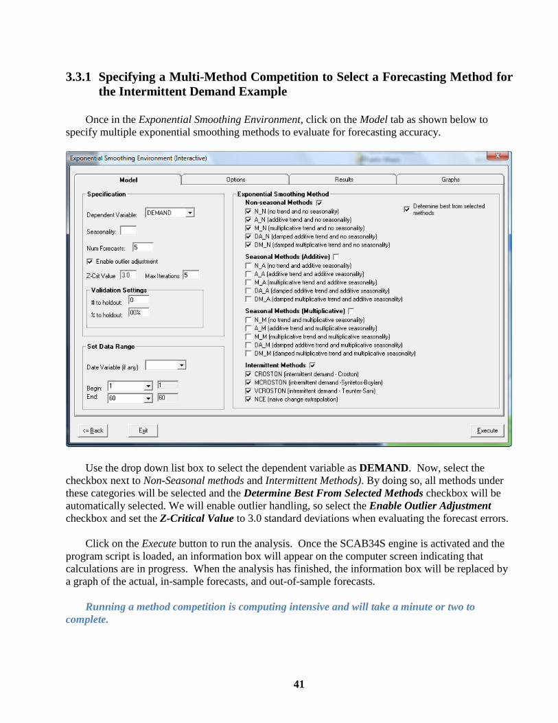
3.3.1 Specifying a Multi-Method Competition to Select a Forecasting Method for
the Intermittent Demand Example
Once in the Exponential Smoothing Environment, click on the Model tab as shown below to
specify multiple exponential smoothing methods to evaluate for forecasting accuracy.
Use the drop down list box to select the dependent variable as DEMAND. Now, select the
checkbox next to Non-Seasonal methods and Intermittent Methods). By doing so, all methods under
these categories will be selected and the Determine Best From Selected Methods checkbox will be
automatically selected. We will enable outlier handling, so select the Enable Outlier Adjustment
checkbox and set the Z-Critical Value to 3.0 standard deviations when evaluating the forecast errors.
Click on the Execute button to run the analysis. Once the SCAB34S engine is activated and the
program script is loaded, an information box will appear on the computer screen indicating that
calculations are in progress. When the analysis has finished, the information box will be replaced by
a graph of the actual, in-sample forecasts, and out-of-sample forecasts.
Running a method competition is computing intensive and will take a minute or two to
complete.
42
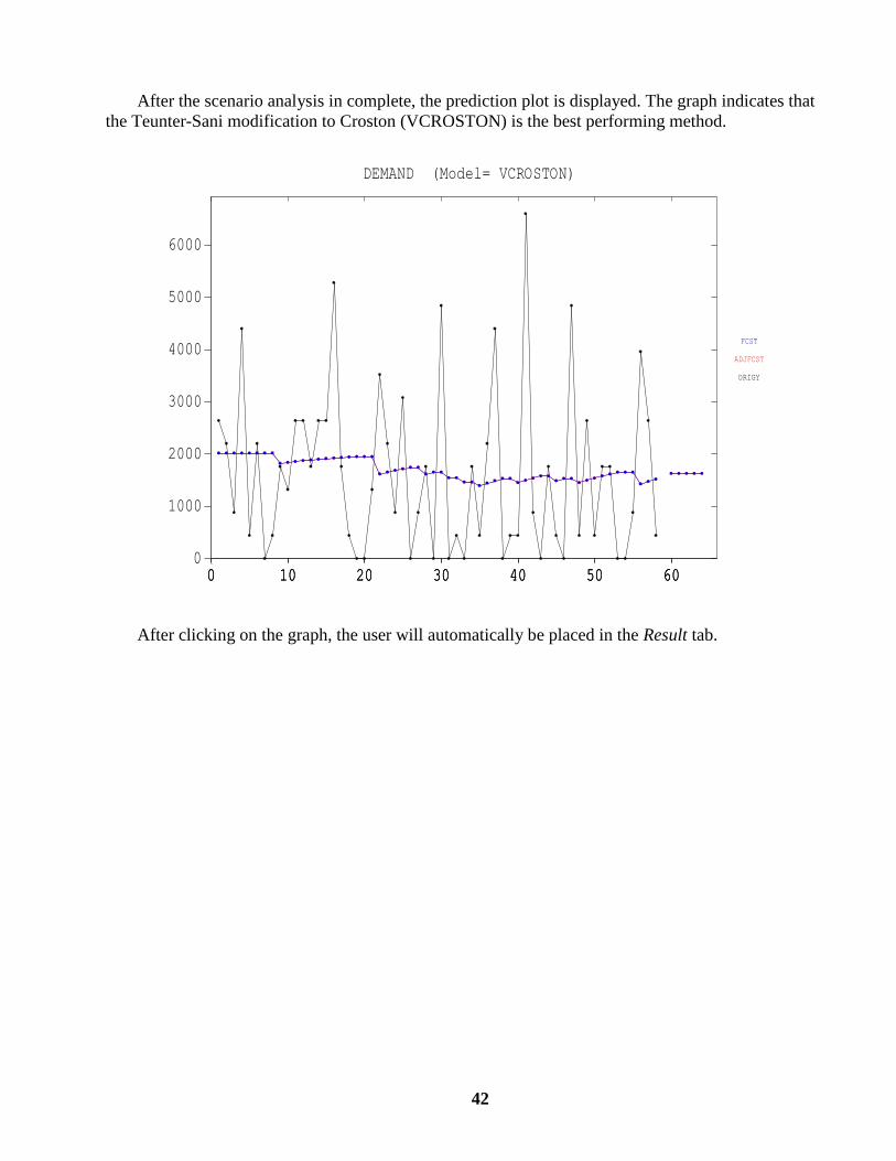
After the scenario analysis in complete, the prediction plot is displayed. The graph indicates that
the Teunter-Sani modification to Croston (VCROSTON) is the best performing method.
DEMAND (Model= VCROSTON)
0 10 20 30 40 50 600 10 20 30 40 50 600
1000
2000
3000
4000
5000
6000
0 10 20 30 40 50 60
ORIGY
ADJFCST
FCST
After clicking on the graph, the user will automatically be placed in the Result tab.
43
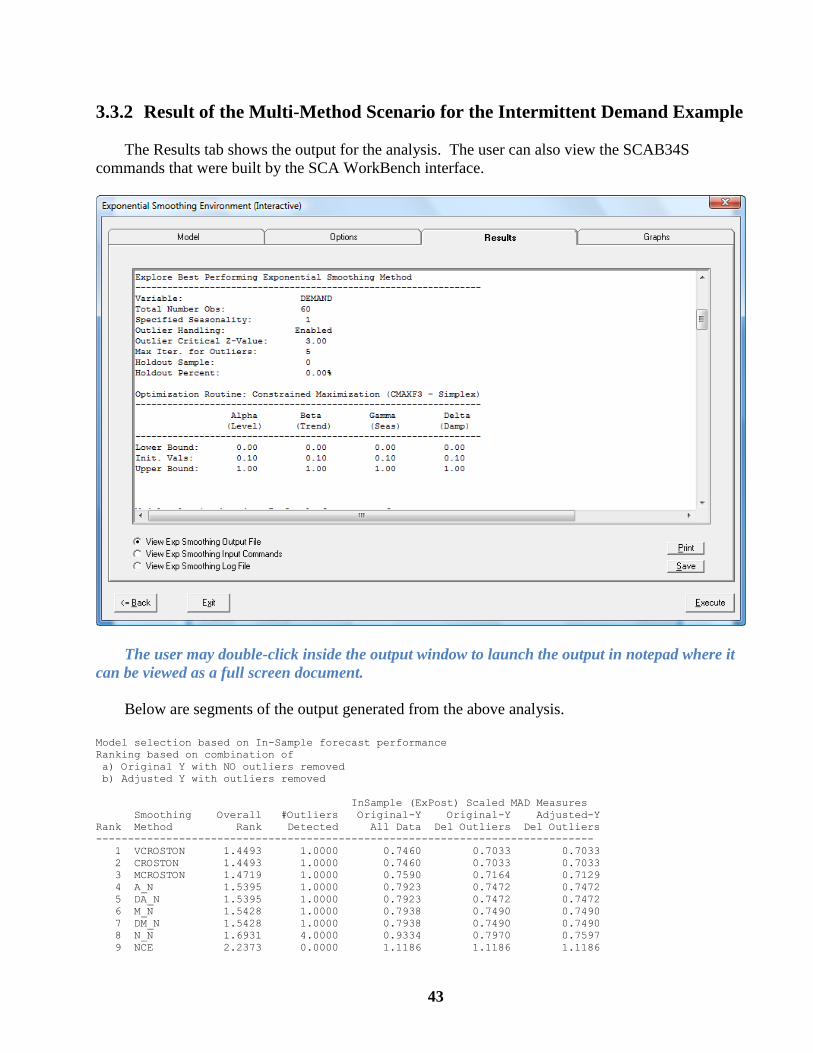
3.3.2 Result of the Multi-Method Scenario for the Intermittent Demand Example
The Results tab shows the output for the analysis. The user can also view the SCAB34S
commands that were built by the SCA WorkBench interface.
The user may double-click inside the output window to launch the output in notepad where it
can be viewed as a full screen document.
Below are segments of the output generated from the above analysis.
Model selection based on In-Sample forecast performance
Ranking based on combination of
a) Original Y with NO outliers removed
b) Adjusted Y with outliers removed
InSample (ExPost) Scaled MAD Measures
Smoothing Overall #Outliers Original-Y Original-Y Adjusted-Y
Rank Method Rank Detected All Data Del Outliers Del Outliers
------------------------------------------------------------------------------
1 VCROSTON 1.4493 1.0000 0.7460 0.7033 0.7033
2 CROSTON 1.4493 1.0000 0.7460 0.7033 0.7033
3 MCROSTON 1.4719 1.0000 0.7590 0.7164 0.7129
4 A_N 1.5395 1.0000 0.7923 0.7472 0.7472
5 DA_N 1.5395 1.0000 0.7923 0.7472 0.7472
6 M_N 1.5428 1.0000 0.7938 0.7490 0.7490
7 DM_N 1.5428 1.0000 0.7938 0.7490 0.7490
8 N_N 1.6931 4.0000 0.9334 0.7970 0.7597
9 NCE 2.2373 0.0000 1.1186 1.1186 1.1186
44
The Alpha and Beta smoothing constants for the CROSTON, MCROSTON, and
VCROSTON methods are both for Level. However, Alpha controls level adjustment for
the non-zero demand periods and Beta controls level adjustment for the inter-arrival
periods between non-zero demands.
Final Optimization Results for Smoothing Constants by Ranked Model
----------------------------------------------------------
Rank Method Alpha Beta Gamma Delta
(Level) (Trend) (Seas) (Damp)
----------------------------------------------------------
1 VCROSTON 0.0000 0.1078
2 CROSTON 0.0000 0.1077
3 MCROSTON 0.0863
4 A_N 0.0000 0.4957
5 DA_N 0.0000 0.3798 1.0000
6 M_N 0.0000 0.4957
7 DM_N 0.0000 0.1301 1.0000
8 N_N 0.0955
9 NCE
Variable: DEMAND
Total Number Obs: 60
Specified Seasonality: 1
Exponential Smoothing Method: VCRO
Intermittency: Teunter-Sani (2009) Intermittent Demand Method
Outlier Handling: Enabled
Outlier Critical Z-Value: 3.00
Max Iter. for Outliers: 5
Obs Used to Initialize: 60
Holdout Sample: 0
Holdout Percent: 0.00%
Number of Forecasts: 5
The estimation results for the smoothing constants of the winning method is displayed next. The
mean absolute deviation scaled by the overall mean of the target time series is used as the
performance measure.
Smoothing Constant Initialization and Constraints
Optimization Routine: Pre-specified smoothing constants
-----------------------------------------------------------------
Alpha Beta Gamma Delta
(Level) (Trend) (Seas) (Damp)
-----------------------------------------------------------------
Lower Bound: 0.00 0.00 0.00 0.00
Init. Vals: 0.10 0.10 0.10 0.10
Upper Bound: 1.00 1.00 1.00 1.00
Start Vals: 2017. 1.000 na na
Final Optimization Results for Smoothing Constants
-------------------------------------------------------
Smoothing Alpha Beta Gamma Delta
Constants (Level) (Trend) (Seas) (Damp)
-------------------------------------------------------
Unadjusted : 0.0000 0.1078
Adjusted : 0.0000 0.1078
Forecast Performance (ExPost - Insample)
----------------------------------------------
Number of cases: 58
Scaled MAD (Unadjusted): 0.7460
Scaled MAD (Adjusted Coefficients): 0.7033
Scaled MAD (Adjusted Y and Coeffs): 0.7033
Number of outliers detected: 1
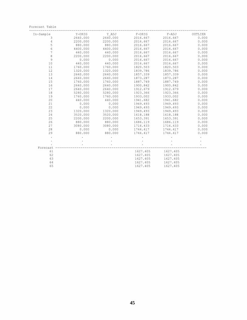
45
Forecast Table
--------------------------------------------------------------------------------------------
In-Sample Y-ORIG Y_ADJ F-ORIG F-ADJ OUTLIER
3 2640.000 2640.000 2016.667 2016.667 0.000
4 2200.000 2200.000 2016.667 2016.667 0.000
5 880.000 880.000 2016.667 2016.667 0.000
6 4400.000 4400.000 2016.667 2016.667 0.000
7 440.000 440.000 2016.667 2016.667 0.000
8 2200.000 2200.000 2016.667 2016.667 0.000
9 0.000 0.000 2016.667 2016.667 0.000
10 440.000 440.000 2016.667 2016.667 0.000
11 1760.000 1760.000 1820.503 1820.503 0.000
12 1320.000 1320.000 1839.786 1839.786 0.000
13 2640.000 2640.000 1857.339 1857.339 0.000
14 2640.000 2640.000 1873.287 1873.287 0.000
15 1760.000 1760.000 1887.749 1887.749 0.000
16 2640.000 2640.000 1900.842 1900.842 0.000
17 2640.000 2640.000 1912.679 1912.679 0.000
18 5280.000 5280.000 1923.366 1923.366 0.000
19 1760.000 1760.000 1933.002 1933.002 0.000
20 440.000 440.000 1941.682 1941.682 0.000
21 0.000 0.000 1949.493 1949.493 0.000
22 0.000 0.000 1949.493 1949.493 0.000
23 1320.000 1320.000 1949.493 1949.493 0.000
24 3520.000 3520.000 1618.188 1618.188 0.000
25 2200.000 2200.000 1653.391 1653.391 0.000
26 880.000 880.000 1686.119 1686.119 0.000
27 3080.000 3080.000 1716.433 1716.433 0.000
28 0.000 0.000 1744.417 1744.417 0.000
29 880.000 880.000 1744.417 1744.417 0.000
. . . . . .
. . . . . .
. . . . . .
Forecast ------------------------------------------------------------------------------
61 1627.405 1627.405
62 1627.405 1627.405
63 1627.405 1627.405
64 1627.405 1627.405
65 1627.405 1627.405

46
By clicking on the Graph tab, the user can examine various graphs including a time plot of the
dependent variable, actual versus predicted, forecast plot, time plots of residuals, residual
autocorrelation function, Q-Stat charts.
The user may double-click on the graph to launch the graph in Microsoft Graphics Manager
where it can be viewed as a full screen document.

47
4 A DETAILED DESCRIPTION OF THE SMOOTH ROUTINE
The SCAB34S product implements all exponential smoothing methods described in Gardner
(2006) and then some. A detailed description of the SMOOTH subroutine is listed below. This
subroutine is wrapped by other routines used inside the Exponential Smoothing application
environment of SCA WorkBench.
Usage:
CALL SMOOTH(Y :OPTIONS);
Note if :method key is supplied it MUST be the first option specified after the variable name.
Required subroutine arguments:
Arguments Intent Comments
Y Input Target variable to apply exponential smoothing.
Optional keywords and associated arguments:
Keyword #
Args
Type(s) Intent Comments
:METHOD 1 Character
keyword
input Specifies the exponential smoothing method to be
executed. The methods supported are
NCE No change extrapolation (default)
NCEPT No change extrap. Plus trend
AVETD Average-to-date
MAVE Moving average
DMAVE Double moving average
N_N Simple exponential smoothing
A_N Holt’s additive trend
M_N Pegel’s multiplicative trend
DA_N Damped Holt’s additive trend
DM_N Damped Pegel’s multiplicative trend
N_A No trend with additive seasonality
A_A Additive Holt-Winters
M_A Trend=Mult., Seas=Additive
DA_A Damped Additive Holt-Winters
DM_A Trend=Damped Mult, Seas=Additive
N_M No trend with multiplicative seasonality
A_M Multiplicative Holt-Winters
M_M Trend=Mult., Seas=Multiplicative
DA_M Damped Multiplicative Holt-Winters
DM_M Trend=Damped Mult, Seas=Mult.
CROSTON Intermittent by Croston
MCROSTON Intermittent by Teunter-Sani
VCROSTON Intermittent by Syntetos -Boylan
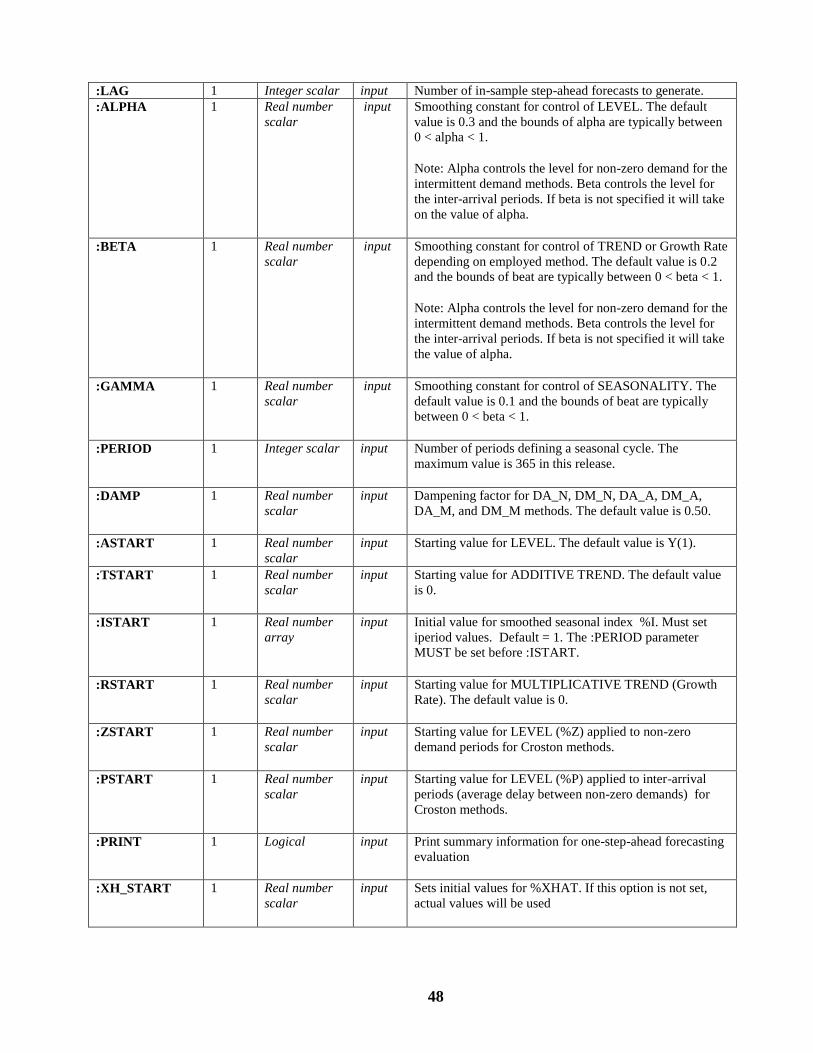
48
:LAG 1 Integer scalar input Number of in-sample step-ahead forecasts to generate.
:ALPHA 1 Real number
scalar
input Smoothing constant for control of LEVEL. The default
value is 0.3 and the bounds of alpha are typically between
0 < alpha < 1.
Note: Alpha controls the level for non-zero demand for the
intermittent demand methods. Beta controls the level for
the inter-arrival periods. If beta is not specified it will take
on the value of alpha.
:BETA 1 Real number
scalar
input Smoothing constant for control of TREND or Growth Rate
depending on employed method. The default value is 0.2
and the bounds of beat are typically between 0 < beta < 1.
Note: Alpha controls the level for non-zero demand for the
intermittent demand methods. Beta controls the level for
the inter-arrival periods. If beta is not specified it will take
the value of alpha.
:GAMMA 1 Real number
scalar
input Smoothing constant for control of SEASONALITY. The
default value is 0.1 and the bounds of beat are typically
between 0 < beta < 1.
:PERIOD 1 Integer scalar input Number of periods defining a seasonal cycle. The
maximum value is 365 in this release.
:DAMP 1 Real number
scalar
input Dampening factor for DA_N, DM_N, DA_A, DM_A,
DA_M, and DM_M methods. The default value is 0.50.
:ASTART 1 Real number
scalar
input Starting value for LEVEL. The default value is Y(1).
:TSTART 1 Real number
scalar
input Starting value for ADDITIVE TREND. The default value
is 0.
:ISTART 1 Real number
array
input Initial value for smoothed seasonal index %I. Must set
iperiod values. Default = 1. The :PERIOD parameter
MUST be set before :ISTART.
:RSTART 1 Real number
scalar
input Starting value for MULTIPLICATIVE TREND (Growth
Rate). The default value is 0.
:ZSTART 1 Real number
scalar
input Starting value for LEVEL (%Z) applied to non-zero
demand periods for Croston methods.
:PSTART 1 Real number
scalar
input Starting value for LEVEL (%P) applied to inter-arrival
periods (average delay between non-zero demands) for
Croston methods.
:PRINT 1 Logical input Print summary information for one-step-ahead forecasting
evaluation
:XH_START 1 Real number
scalar
input Sets initial values for %XHAT. If this option is not set,
actual values will be used

49
:AUTOFIX 1 Logical input Automatically corrects bounds errors for ALPHA, BETA,
GAMMA and DAMP. Note the following allowed ranges:
ALPHA bounds 0. - 2. for N_N, A_N and M_N
ALPHA bounds 0. – 1. otherwise
BETA bounds 0. - 1.
GAMMA bounds 0. - 1.
DAMP bounds 0. - 1.
:AUTOFIX should be specified after :METHOD key and
is useful when estimating the smoothing constants using
CMAXF2, CMAXF3, or CMAXSEARCH optimization.
:FORECAST 1 Integer scalar input Number of forecasts to generate off the end of the series.
:TMAX 1 Real number
scalar
input Sets an absolute value on %T for methods M_N, M_A,
M_M, DM_N, DM_A, and DM_M
%T has a lower bound of 0.0 to avoid entering the
complex domain
Variables created in SMOOTH subroutine call:
Variable Comments
%XHATMAT Real number array; output only
In-Sample forecasts beginning with smoothed Y, and followed by forecasts at t=1 to t=m.
Missing rows occur that contain artificial observations used as starting values.
Note that these forecasts are recursively calculated.
%XHAT Real number array; output only
In-Sample forecasts for one-step-ahead forecasts lined up with Y
Note that these forecasts are recursively calculated.
%XHATOBS Real number array; output only
Observation numbers aligned to %XHAT
%SOBS Real number array; output only
Observation numbers aligned to %S
%S Real number array; output only
Iterative values of LEVEL used in the forecast function
%ACTUAL Real number array; output only
Actual Y values aligned to %SOBS
%T Real number array; output only
Iterative values of TREND used in the forecast function for additive trend methods
%R Real number array; output only
Iterative values of GROWTH RATE used in the forecast function for multiplicative trend
methods
%I Real number array; output only
Iterative values of SEASONAL INDEX used in the forecast function for seasonal methods
%Z Real number array; output only
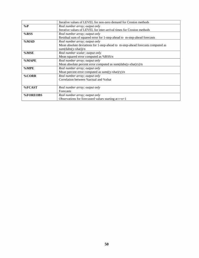
50
Iterative values of LEVEL for non-zero demand for Croston methods
%P Real number array; output only
Iterative values of LEVEL for inter-arrival times for Croston methods
%RSS Real number array; output only
Residual sum of squared error for 1-step-ahead to m-step-ahead forecasts
%MAD Real number array; output only
Mean absolute deviations for 1-step-ahead to m-step-ahead forecasts computed as
sum(dabs(y-xhat))/n
%MSE Real number scalar; output only
Mean squared error computed as %RSS/n
%MAPE Real number array; output only
Mean absolute percent error computed as sum(dabs(y-xhat)/y)/n
%MPE Real number array; output only
Mean percent error computed as sum((y-xhat)/y)/n
%CORR Real number array; output only
Correlation between %actual and %xhat
%FCAST Real number array; output only
Forecasts
%FOREOBS Real number array; output only
Observations for forecasted values starting at t=n+1

51
5 A DETAILED DESCRIPTION OF CUSTOMIZABLE SUBROUTINES
USED IN THE EXPONENTIAL SMOOTHING APPLICATION
The SCAB34S exponential smoothing application uses some customized subroutines that were
developed in the B34S matrix language. These subroutines perform similar to a macro procedure and
are stored in the STAGING.MAC, WBSUPPL.MAC, and EXSMOOTH.MAC files located in the
B34SLM installation folder. Since these subroutines are loaded and called from the script generated
by SCA WorkBench for exponential smoothing modeling, the user can modify the scripts to handle
some specific needs, as long as the nature of the arguments and calling sequence of the arguments is
not changed.
It is highly recommended that you make a backup of the original files before attempting to customize
the subroutines.
5.1 INIEXPSM User Program
The INIEXPSM program is an external routine located in the ExSmooth.MAC file. This routine
initializes the global arguments used throughout the SCA WorkBench Exponential Smoothing
application environment. These initial settings can be overridden by the user by changing the values
of these arguments after the INIEXPSM program is executed or by modifying the INIEXPSM
program itself.
Usage:
CALL INIEXPSM;
Initialized Global Arguments:
Arguments Type(s) Intent Comments
%ESMODEL CHAR*8 Global argument The character key for the exponential smoothing
method. Default set to
%ESMODEL=’N_N’
%SPANINI Integer scalar Global argument Use observation 1 - %SPANINI to initialize
starting values for level, trend, and season. Default
set to
%SPANINI=1
%HOLDOUT Real number
scalar
Global argument Percent of series to hold out for %EXANTE.
Typical values range from 0.0 - 0.50. Default set to
%HOLDOUT=0.25
%SPANOPT(2) Real number
vector
Global argument Use observation span %SPANOPT(1) -
%SPANOPT(2) to optimize smoothing constants.
Only element %SPANOPT(1) is set by
INIEXPSM since the ending span %SPANOPT(2)
is dependent upon the number of observations in
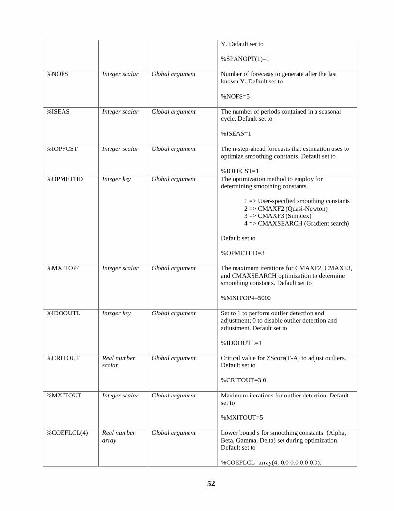
52
Y. Default set to
%SPANOPT(1)=1
%NOFS Integer scalar Global argument Number of forecasts to generate after the last
known Y. Default set to
%NOFS=5
%ISEAS Integer scalar Global argument The number of periods contained in a seasonal
cycle. Default set to
%ISEAS=1
%IOPFCST Integer scalar Global argument The n-step-ahead forecasts that estimation uses to
optimize smoothing constants. Default set to
%IOPFCST=1
%OPMETHD Integer key Global argument The optimization method to employ for
determining smoothing constants.
1 => User-specified smoothing constants
2 => CMAXF2 (Quasi-Newton)
3 => CMAXF3 (Simplex)
4 => CMAXSEARCH (Gradient search)
Default set to
%OPMETHD=3
%MXITOP4 Integer scalar Global argument The maximum iterations for CMAXF2, CMAXF3,
and CMAXSEARCH optimization to determine
smoothing constants. Default set to
%MXITOP4=5000
%IDOOUTL Integer key Global argument Set to 1 to perform outlier detection and
adjustment; 0 to disable outlier detection and
adjustment. Default set to
%IDOOUTL=1
%CRITOUT Real number
scalar
Global argument Critical value for ZScore(F-A) to adjust outliers.
Default set to
%CRITOUT=3.0
%MXITOUT Integer scalar Global argument Maximum iterations for outlier detection. Default
set to
%MXITOUT=5
%COEFLCL(4) Real number
array
Global argument Lower bound s for smoothing constants (Alpha,
Beta, Gamma, Delta) set during optimization.
Default set to
%COEFLCL=array(4: 0.0 0.0 0.0 0.0);

53
%COEFUCL(4) Real number
array
Global argument Upper bound s for smoothing constants (Alpha,
Beta, Gamma, Delta) set during optimization.
Default set to
%COEFUCL=array(4: 1.0 1.0 1.0 1.0)
%COEFS(4,2) Real number
array
Global argument The smoothing constants either passed into the
routine as user-specified values or returned from
the routine as optimized values. The array consists
of 4 columns corresponding to alpha, beta, gamma,
and delta. The rows correspond to unadjusted
values for the smoothing constants and outlier
adjusted values, respectively. Default set to
%COEFS=
array(4,2: 0.3 missing() missing() missing()
missing() missing() missing() missing())
%IPRINT Integer key Global argument Turns on/off printing of additional information
during optimization of smoothing constants.
Setting %IPRINT=0 turns off additional printing
and %IPRINT=1 turns on printing. Default set to
%IPRINT=0
%ERRTRAP Integer key Global argument Turns on/off error messages related to debugging.
The user usually will not need to set this option
unless the user is familiar with B34S matrix
commands and is able to debug the ExSmooth.mac
command files. %ERRTRAP=0 turns trapping
off. Default set to
%ERRTRAP=1
%RANKWGT(3) Real number
array
Global argument Allows user to modify weighting scheme for
model ranking in the AUTOES1 routine.
%RANKWGT(1) => 0.0 system default,
1.0 user specified
%RANKWGT(2) => Weight assigned to out-of-
sample performance (between 0.0 – 1.0).
%RANKWGT(3) => Weight assigned to outlier
adjusted performance (between 0.0 – 1.0).
5.2 SETEXPSM User Program
The SETXPSM program is an external routine located in the ExSmooth.MAC file. This routine
sets the starting values and data span for determining the smoothing constants based on the
exponential smoothing method specified by the global %ESMODEL argument. Depending on the
54
exponential smoothing method, starting values may be obtains by OLS estimation, sample mean,
sample median, or other. The user can override the starting values for level, trend, and seasonality by
resetting %STARTVL1, %STARTVL2, and %STARTVL3 after running SETEXPSM. The user may
also modify the SETEXPSM routine directly for a permanent modification to be in effect.
Usage:
%ESMODEL=1;
CALL INIEXPSM;
5.3 RUNEXPSM User Program
The RUNEXPSM program is an external routine located in the ExSmooth.MAC file. This
routine is a super-routine that shells the EXPSM subroutine. Based on the value of the global
argument %ESMODEL, the corresponding %IMODEL value is set, data integrity is checked to make
sure the method can be applied, and finally the EXPSM subroutine is called.
Usage:
%ESMODEL=1;
CALL RUNEXPSM;
5.4 DSPEXPSM User Program
The DSPEXPSM program is an external routine located in the ExSmooth.MAC file. This routine
prints the results for a single exponential smoothing run and is designed to organize and display
various global arguments set by the user and derived by the RUNEXPSM call.
Usage:
CALL RUNEXPSM;
CALL DSPEXPSM;
5.5 GRFEXPS1 User Program
The GRFEXPS1 program is an external routine located in the ExSmooth.MAC file. This routine
graphs the results for a single exponential smoothing after the RUNEXPSM call. The hard copy of
the file is saved to the name esfcast.wmf which is in windows meta file format. Note, an alternative
GRFEXPSM program will save the file based on the target series name.
Usage:
CALL RUNEXPSM;
CALL GRFEXPS1;
55
5.6 AUTOEXP1 User Program
The AUTOEXP1 program is an external routine located in the ExSmooth.MAC file. This is a
super-routine that will run multiple exponential smoothing methods, rank the methods according to
in-sample or out-of-sample forecasting performance, and print the ranked results. This program
requires an array %ESTEST to be set prior to its execution. The %ESTEST array contains the
CHAR*8 names of the exponential smoothing methods to be evaluated and ranked.
The complete results of the method competition (performance measures, smoothing constants,
and rank) are saved to the %ESEVAL(p,14) array where row (p) corresponds to the model key. The
columns are defined as
Column Description
1 Model Key (see %IMODEL description in EXPSM routine)
2 Scaled MAD for in-sample (Ex-Post) Original Y, outliers not removed
3 Scaled MAD for in-sample (Ex-Post) Original Y, outliers removed
4 Scaled MAD for in-sample (Ex-Post) Adjusted Y, outliers removed
5 Scaled MAD for out-of-sample (Ex-Ante) Original Y, outliers not removed
6 Scaled MAD for out-of-sample (Ex-Ante) Original Y, outliers removed
7 Scaled MAD for out-of-sample (Ex-Ante) Adjusted Y, outliers removed
8 Number of outliers detected for in-sample (Ex-Post) periods
9 Number of outliers detected for out-of-samples (Ex-Ante) periods
10 Adjusted Alpha (smoothing constant for level)
11 Adjusted Beta (smoothing constant for trend or growth rate)
12 Adjusted Gamma (smoothing constant for seasonality)
13 Adjusted Delta (constant for dampening trend)
14 Overall weighted rank of method
Usage:
%ESTEST=array(5: 'N_N', 'A_N', 'M_N', 'DA_N', 'DM_N');
CALL AUTOEXP1;
5.7 EXPSM User Subroutine
The EXPSM routine is an external subroutine located in the ExSmooth.MAC file. This routine is
the key subroutine that supports the SCA WorkBench Exponential Smoothing application
environment. It will execute a single exponential smoothing method. Other routines in the
ExSmooth.MAC file are used to setup and shell the EXPSM call including super-routines that setup
the environment for the smoothing method (e.g., starting values) and/or iteratively call EXPSM for
multi-method exploration.
Usage:

56
CALL LOAD(EXPSM ‘C:\SCA\B34SLM\LIB\EXSMOOTH.MAC’);
%IMODEL=1;
CALL EXPSM(Y,
%SPANINI,%HOLDOUT,%SPANOPT, %NOFS, %ISEAS,%IOPFCST,
%OPMETHD,%MXITOP4,%IDOOUTL,%CRITOUT,%MXITOUT,%COEFLCL,
%COEFUCL,%COEFINI,%STRTVL1,%STRTVL2,%STRTVL3,%ADJY ,
%FCSTS ,%EXPOST ,%EXANTE , %sMAD1 ,%sMAD2 ,%COEFS ,
%IMODEL ,%IPRINT);

57
Required global arguments:
Arguments Type(s) Intent Comments
%IMODEL Integer key input Sets the exponential smoothing method that is to
be executed by the EXPSM subroutine. This
parameter must be set prior to calling the EXPSM
routine
Key Method
1 N_N
2 A_N
3 M_N
4 DA_N
5 DM_N
6 N_A
7 A_A
8 M_A
9 DA_A
10 DM_A
11 N_M
12 A_M
13 M_M
14 DA_M
15 DM_M
16 CROS
17 MCRO
18 VCRO
19 NCE
Required subroutine arguments:
Arguments Type(s) Intent Comments
Y Real number
vector
input The name of the dependent variable (0-1) in the
model
%SPANINI Integer scalar input Use observation 1 - %SPANINI to initialize
starting values for level, trend, and season
%HOLDOUT Real number
scalar
input Percent of series to hold out for %EXANTE.
Typical values range from 0.0 - 0.50
%SPANOPT(2) Real number
vector
input Use observation span %SPANOPT(1) -
%SPANOPT(2) to optimize smoothing constants
%NOFS Real number
vector
input Number of forecasts to generate after the last
known Y
%ISEAS Integer scalar input Seasonal period (eg., 12=> Monthly, 7=>Daily)
%IOPFCST Integer scalar input N-STEP-AHEAD Forecast to optimize. Typically
set to 1 for 1-step-ahead forecast optimization
%OPMETHD Integer scalar input Optimization method for determining smoothing
constants
1 => User-specified smoothing constants
2 => CMAXF2 (Quasi-Newton)
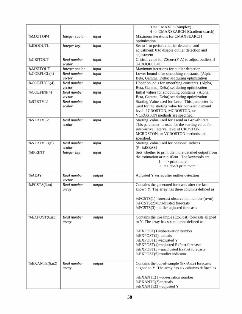
58
3 => CMAXF3 (Simplex)
4 => CMAXSEARCH (Gradient search)
%MXITOP4 Integer scalar input Maximum iterations for CMAXSEARCH
optimization
%IDOOUTL Integer key input Set to 1 to perform outlier detection and
adjustment; 0 to disable outlier detection and
adjustment
%CRITOUT Real number
scalar
input Critical value for ZScore(F-A) to adjust outliers if
%IDOOUTL=1
%MXITOUT Integer scalar input Maximum iterations for outlier detection
%COEFLCL(4) Real number
vector
input Lower bound s for smoothing constants (Alpha,
Beta, Gamma, Delta) set during optimization
%COEFUCL(4) Real number
vector
input Upper bound s for smoothing constants (Alpha,
Beta, Gamma, Delta) set during optimization
%COEFINI(4) Real number
vector
input Initial values for smoothing constants (Alpha,
Beta, Gamma, Delta) set during optimization
%STRTVL1 Real number
scalar
input Starting Value used for Level. This parameter is
used for the starting value for non-zero demand
level if CROSTON, MCROSTON, or
VCROSTON methods are specified.
%STRTVL2 Real number
scalar
input Starting Value used for Trend or Growth Rate.
This parameter is used for the starting value for
inter-arrival interval level)if CROSTON,
MCROSTON, or VCROSTON methods are
specified.
%STRTVL3(P) Real number
scalar
input Starting Value used for Seasonal Indices
(P=%ISEAS)
%IPRINT Integer key input Sets whether to print the more detailed output from
the estimation or run silent. The keywords are
1 => print more
0 => don’t print more
%ADJY Real number
vector
output Adjusted Y series after outlier detection
%FCSTS(3,m) Real number
array
output Contains the generated forecasts after the last
known Y. The array has three columns defined as
%FCSTS(1)=forecast observation number (n+m)
%FCSTS(2)=unadjusted forecasts
%FCSTS(3)=outlier adjusted forecasts
%EXPOST(6,n1) Real number
array
output Contains the in-sample (Ex-Post) forecasts aligned
to Y. The array has six columns defined as
%EXPOST(1)=observation number
%EXPOST(2)=actuals
%EXPOST(3)=adjusted Y
%EXPOST(4)=adjusted ExPost forecasts %EXPOST(5)=unadjusted ExPost forecasts
%EXPOST(6)=outlier indicator
%EXANTE(6,n2) Real number
array
output Contains the out-of-sample (Ex-Ante) forecasts
aligned to Y. The array has six columns defined as
%EXANTE(1)=observation number
%EXANTE(2)=actuals
%EXANTE(3)=adjusted Y
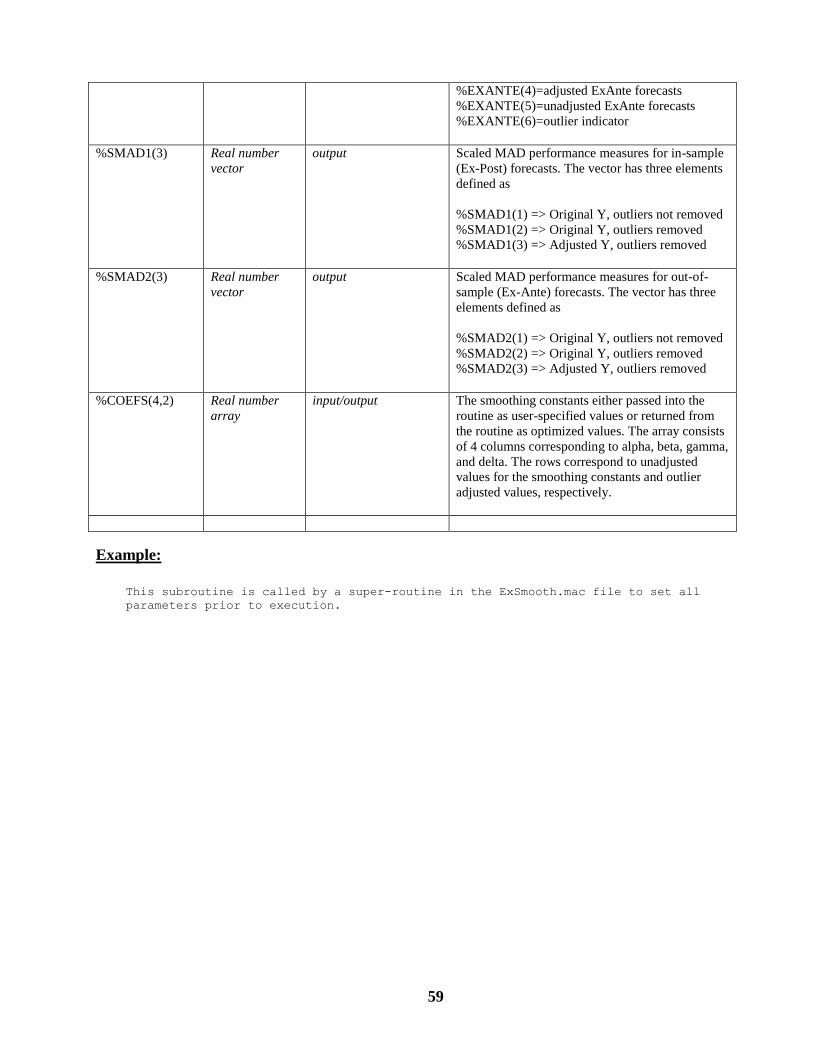
59
%EXANTE(4)=adjusted ExAnte forecasts %EXANTE(5)=unadjusted ExAnte forecasts
%EXANTE(6)=outlier indicator
%SMAD1(3) Real number
vector
output Scaled MAD performance measures for in-sample
(Ex-Post) forecasts. The vector has three elements
defined as
%SMAD1(1) => Original Y, outliers not removed
%SMAD1(2) => Original Y, outliers removed
%SMAD1(3) => Adjusted Y, outliers removed
%SMAD2(3) Real number
vector
output Scaled MAD performance measures for out-of-
sample (Ex-Ante) forecasts. The vector has three
elements defined as
%SMAD2(1) => Original Y, outliers not removed
%SMAD2(2) => Original Y, outliers removed
%SMAD2(3) => Adjusted Y, outliers removed
%COEFS(4,2) Real number
array
input/output The smoothing constants either passed into the
routine as user-specified values or returned from
the routine as optimized values. The array consists
of 4 columns corresponding to alpha, beta, gamma,
and delta. The rows correspond to unadjusted
values for the smoothing constants and outlier
adjusted values, respectively.
Example:
This subroutine is called by a super-routine in the ExSmooth.mac file to set all
parameters prior to execution.
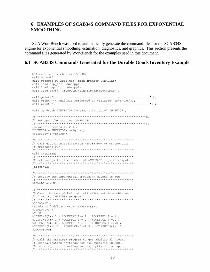
60
6. EXAMPLES OF SCAB34S COMMAND FILES FOR EXPONENTIAL
SMOOTHING
SCA WorkBench was used to automatically generate the command files for the SCAB34S
engine for exponential smoothing, estimation, diagnostics, and graphics. This section presents the
command files generated by WorkBench for the examples used in this document.
6.1 SCAB34S Commands Generated for the Durable Goods Inventory Example
b34sexec matrix cbuffer=150000;
call echooff;
call getsca('DURABLE.mad' :mad :member DURABLE);
call load(dsp_acf :wbsuppl);
call load(dsp_tbl :wbsuppl);
call load(EXPSM 'C:\sca\B34SLM\lib\ExSmooth.mac');
call print('-------------------------------------------------------':);
call print('** Analysis Performed on Variable: INVENTOR':);
call print('-------------------------------------------------------':);
call dspdscrb('INVENTOR Dependent Variable',INVENTOR);
/$ **************************************************************$/
/$ Set span for sample: INVENTOR
/$ **************************************************************$/
iorigins=integers(1, 204);
INVENTOR = INVENTOR(iorigins);
%YSERIES='INVENTOR';
/$ *******************************************************
/$ Call global initialization (INIEXSPM) of exponential
/$ smoothing run.
/$ *******************************************************
call INIEXPSM;
/$ *******************************************************
/$ set _nlags for the number of ACF/PACF lags to compute
/$ *******************************************************
_nlags=12;
/$ *******************************************************
/$ Specify the exponential smoothing method to run
/$ *******************************************************
%ESMODEL='M_N';
/$ *******************************************************
/$ Override some global initialization settings obtained
/$ from the INIEXPSM program
/$ *******************************************************
%ISEAS=12 ;
%holdout=.0/dfloat(norows(INVENTOR));
%OPMETHD=3 ;
%NOFS=5 ;
%COEFINI(1)=.1 ; %COEFINI(2)=.1 ; %COEFINI(3)=.1 ;
%COEFINI(4)=.1 ; %COEFLCL(1)=.0 ; %COEFLCL(2)=.0 ;
%COEFLCL(3)=.0 ; %COEFLCL(4)=.0 ; %COEFUCL(1)=1.0 ;
%COEFUCL(2)=1.0 ; %COEFUCL(3)=1.0 ; %COEFUCL(4)=1.0 ;
%IDOOUTL=0;
/$ *******************************************************
/$ Call the SETEXPSM program to get additional global
/$ initialization settings for the specific %ESMODEL
/$ to be applied (starting values, optimization span)
/$ *******************************************************

61
call SETEXPSM;
/$ *******************************************************
/$ Call the RUNEXPSM program to run the %ESMODEL and
/$ obtain optimized smoothing values, performance measures,
/$ and forecasts
/$ *******************************************************
call RUNEXPSM;
/$ *******************************************************
/$ Call the DSPEXPSM program to display the exponential
/$ smoothing results
/$ *******************************************************
call DSPEXPSM;
/$ *******************************************************
/$ Call the GRFEXPS1 program to graph the exponential
/$ smoothing results
/$ *******************************************************
call GRFEXPS1;
(common commands for additional graphs and diagnostics omitted here but provided later in
this section)
b34srun;
6.2 SCAB34S Commands for the Seasonal Airline Passenger Load Example
b34sexec matrix cbuffer=150000;
call echooff;
call getsca('BJ_G.mad' :mad :member BJ_G);
call load(dsp_acf :wbsuppl);
call load(dsp_tbl :wbsuppl);
call load(EXPSM 'C:\sca\B34SLM\lib\ExSmooth.mac');
call print('-------------------------------------------------------':);
call print('** Analysis Performed on Variable: Y':);
call print('-------------------------------------------------------':);
call dspdscrb('Y Dependent Variable',Y);
/$ **************************************************************$/
/$ Set span for sample: Y
/$ **************************************************************$/
iorigins=integers(1, 144);
Y = Y(iorigins);
%YSERIES='Y';
/$ *******************************************************
/$ Call global initialization (INIEXSPM) of exponential
/$ smoothing run.
/$ *******************************************************
call INIEXPSM;
/$ *******************************************************
/$ set _nlags for the number of ACF/PACF lags to compute
/$ *******************************************************
_nlags=12;
/$ *******************************************************
/$ Specify the exponential smoothing methods to perform
/$ a competition
/$ *******************************************************
%ESTEST=array(: 'N_A', 'A_A', 'M_A', 'DA_A', 'DM_A', 'N_M',
'A_M', 'M_M', 'DA_M', 'DM_M');
/$ *******************************************************
/$ Override some global initialization settings obtained
/$ from the INIEXPSM program
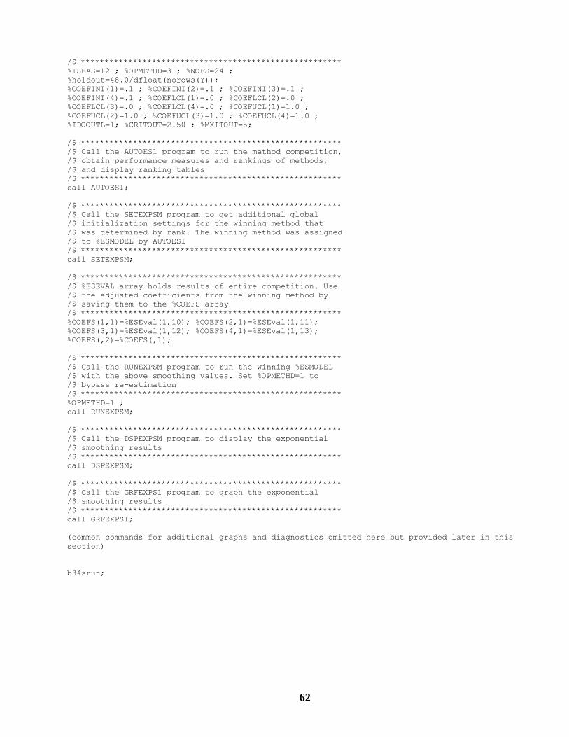
62
/$ *******************************************************
%ISEAS=12 ; %OPMETHD=3 ; %NOFS=24 ;
%holdout=48.0/dfloat(norows(Y));
%COEFINI(1)=.1 ; %COEFINI(2)=.1 ; %COEFINI(3)=.1 ;
%COEFINI(4)=.1 ; %COEFLCL(1)=.0 ; %COEFLCL(2)=.0 ;
%COEFLCL(3)=.0 ; %COEFLCL(4)=.0 ; %COEFUCL(1)=1.0 ;
%COEFUCL(2)=1.0 ; %COEFUCL(3)=1.0 ; %COEFUCL(4)=1.0 ;
%IDOOUTL=1; %CRITOUT=2.50 ; %MXITOUT=5;
/$ *******************************************************
/$ Call the AUTOES1 program to run the method competition,
/$ obtain performance measures and rankings of methods,
/$ and display ranking tables
/$ *******************************************************
call AUTOES1;
/$ *******************************************************
/$ Call the SETEXPSM program to get additional global
/$ initialization settings for the winning method that
/$ was determined by rank. The winning method was assigned
/$ to %ESMODEL by AUTOES1
/$ *******************************************************
call SETEXPSM;
/$ *******************************************************
/$ %ESEVAL array holds results of entire competition. Use
/$ the adjusted coefficients from the winning method by
/$ saving them to the %COEFS array
/$ *******************************************************
%COEFS(1,1)=%ESEval(1,10); %COEFS(2,1)=%ESEval(1,11);
%COEFS(3,1)=%ESEval(1,12); %COEFS(4,1)=%ESEval(1,13);
%COEFS(,2)=%COEFS(,1);
/$ *******************************************************
/$ Call the RUNEXPSM program to run the winning %ESMODEL
/$ with the above smoothing values. Set %OPMETHD=1 to
/$ bypass re-estimation
/$ *******************************************************
%OPMETHD=1 ;
call RUNEXPSM;
/$ *******************************************************
/$ Call the DSPEXPSM program to display the exponential
/$ smoothing results
/$ *******************************************************
call DSPEXPSM;
/$ *******************************************************
/$ Call the GRFEXPS1 program to graph the exponential
/$ smoothing results
/$ *******************************************************
call GRFEXPS1;
(common commands for additional graphs and diagnostics omitted here but provided later in this
section)
b34srun;
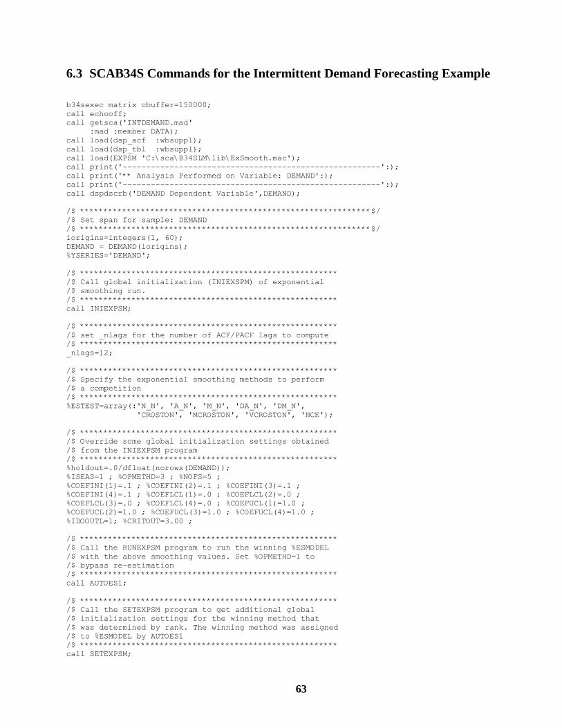
63
6.3 SCAB34S Commands for the Intermittent Demand Forecasting Example
b34sexec matrix cbuffer=150000;
call echooff;
call getsca('INTDEMAND.mad'
:mad :member DATA);
call load(dsp_acf :wbsuppl);
call load(dsp_tbl :wbsuppl);
call load(EXPSM 'C:\sca\B34SLM\lib\ExSmooth.mac');
call print('-------------------------------------------------------':);
call print('** Analysis Performed on Variable: DEMAND':);
call print('-------------------------------------------------------':);
call dspdscrb('DEMAND Dependent Variable',DEMAND);
/$ **************************************************************$/
/$ Set span for sample: DEMAND
/$ **************************************************************$/
iorigins=integers(1, 60);
DEMAND = DEMAND(iorigins);
%YSERIES='DEMAND';
/$ *******************************************************
/$ Call global initialization (INIEXSPM) of exponential
/$ smoothing run.
/$ *******************************************************
call INIEXPSM;
/$ *******************************************************
/$ set _nlags for the number of ACF/PACF lags to compute
/$ *******************************************************
_nlags=12;
/$ *******************************************************
/$ Specify the exponential smoothing methods to perform
/$ a competition
/$ *******************************************************
%ESTEST=array(:'N_N', 'A_N', 'M_N', 'DA_N', 'DM_N',
'CROSTON', 'MCROSTON', 'VCROSTON', 'NCE');
/$ *******************************************************
/$ Override some global initialization settings obtained
/$ from the INIEXPSM program
/$ *******************************************************
%holdout=.0/dfloat(norows(DEMAND));
%ISEAS=1 ; %OPMETHD=3 ; %NOFS=5 ;
%COEFINI(1)=.1 ; %COEFINI(2)=.1 ; %COEFINI(3)=.1 ;
%COEFINI(4)=.1 ; %COEFLCL(1)=.0 ; %COEFLCL(2)=.0 ;
%COEFLCL(3)=.0 ; %COEFLCL(4)=.0 ; %COEFUCL(1)=1.0 ;
%COEFUCL(2)=1.0 ; %COEFUCL(3)=1.0 ; %COEFUCL(4)=1.0 ;
%IDOOUTL=1; %CRITOUT=3.00 ;
/$ *******************************************************
/$ Call the RUNEXPSM program to run the winning %ESMODEL
/$ with the above smoothing values. Set %OPMETHD=1 to
/$ bypass re-estimation
/$ *******************************************************
call AUTOES1;
/$ *******************************************************
/$ Call the SETEXPSM program to get additional global
/$ initialization settings for the winning method that
/$ was determined by rank. The winning method was assigned
/$ to %ESMODEL by AUTOES1
/$ *******************************************************
call SETEXPSM;
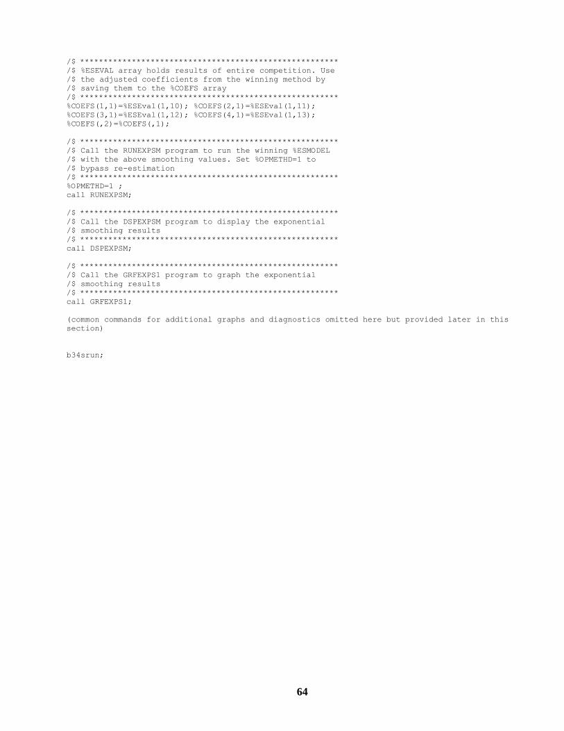
64
/$ *******************************************************
/$ %ESEVAL array holds results of entire competition. Use
/$ the adjusted coefficients from the winning method by
/$ saving them to the %COEFS array
/$ *******************************************************
%COEFS(1,1)=%ESEval(1,10); %COEFS(2,1)=%ESEval(1,11);
%COEFS(3,1)=%ESEval(1,12); %COEFS(4,1)=%ESEval(1,13);
%COEFS(,2)=%COEFS(,1);
/$ *******************************************************
/$ Call the RUNEXPSM program to run the winning %ESMODEL
/$ with the above smoothing values. Set %OPMETHD=1 to
/$ bypass re-estimation
/$ *******************************************************
%OPMETHD=1 ;
call RUNEXPSM;
/$ *******************************************************
/$ Call the DSPEXPSM program to display the exponential
/$ smoothing results
/$ *******************************************************
call DSPEXPSM;
/$ *******************************************************
/$ Call the GRFEXPS1 program to graph the exponential
/$ smoothing results
/$ *******************************************************
call GRFEXPS1;
(common commands for additional graphs and diagnostics omitted here but provided later in this
section)
b34srun;
65
6.4 SCAB34S Commands Used to Display Graphs in the Examples
/$ *******************************************************
/$ Display additional graphics
/$ *******************************************************
_actual=vfam(%EXPOST(,3));
_fcsts=vfam(%EXPOST(,5));
call graph(_actual,_fcsts :file 'yfit.wmf'
:heading 'Original vs. Predicted' :nolabel
:colors black bred bblue);
res1=vfam(_fcsts - _actual);
call dspdscrb('Exp Smoothing Residuals',res1);
/$ **************************************************************$/
/$ Compute ACF, PACF, Q-stats for INVENTOR
/$ **************************************************************$/
call dsp_acf('Actuals',_actual,_nlags,acfy,pacfy,sey,
mqy,pmqy,-1,0,0);
/$ **************************************************************$/
/$ Compute ACF, PACF, Q-stats for model residuals
/$ **************************************************************$/
call dsp_acf('Residuals',res1,_nlags,acfa,pacfa,sea,
mqa,pmqa,-1,0,0);
/$ *******************************************************
/$ Display graphics for Dependent Variable
/$ *******************************************************
call graph(INVENTOR :file 'yvar.wmf' :noshow
:pspaceon
:pgyscaleright 'i'
:pgborder
:pgxscaletop 'i'
:nocontact
:colors black bblue
:heading 'Plot of INVENTOR');
call graph(acfy, sey :file 'acfy.wmf' :noshow
:pspaceon
:pgyscaleright 'i'
:pgborder
:pgxscaletop 'i'
:histscale integers(0,_nlags,2)
:overlay acfplot
:colors black bblue bred
:heading 'ACF of INVENTOR');
call graph(pacfy, sey :file 'pacfy.wmf' :noshow
:pspaceon
:pgyscaleright 'i'
:pgborder
:pgxscaletop 'i'
:histscale integers(0,_nlags,2)
:overlay acfplot
:colors black bblue bred
:heading 'PACF of INVENTOR');
call graph(mqy :file 'mqy.wmf' :noshow
:pspaceon
:pgyscaleright 'i'
:pgborder
:pgxscaletop 'i'
:nocontact
:colors black bblue
:heading 'Q-Stats from INVENTOR');
/$*******************************************************
/$ Display graphics for Exp Smoothing Residuals
66
/$ *******************************************************
call graph(res1 :file 'resa.wmf' :noshow
:pspaceon
:pgyscaleright 'i'
:pgborder
:pgxscaletop 'i'
:nocontact
:colors black bblue
:heading 'Plot of Exp Smoothing Model Residuals');
call graph(acfa, sea :file 'acfa.wmf' :noshow
:pspaceon
:pgyscaleright 'i'
:pgborder
:pgxscaletop 'i'
:histscale integers(0,_nlags,2)
:overlay acfplot
:colors black bblue bred
:heading 'ACF of Exp Smoothing Residuals');
call graph(mqa :file 'mqa.wmf' :noshow
:pspaceon
:pgyscaleright 'i'
:pgborder
:pgxscaletop 'i'
:nocontact
:colors black bblue
:heading 'Q-Stats from Exp Smoothing Residuals');
67
REFERENCES
Brown, R.G. (1959). Statistical Forecasting for Inventory Control, New York: McGraw-Hill.
Croston JF (1972). Forecasting and stock control for intermittent demands.
Operational Research Quarterly, 23, 289-304.
Gardner Jr., E.S. (1985). Exponential smoothing: The state of the art, Journal of Forecasting,
4, 1-28.
Gardner Jr., E.S. & McKenzie, E. (1988). Model identification in exponential smoothing,
Journal of the Operational Research Society, 39, 863-867.
Gardner Jr., E. S. (2006). Exponential smoothing: The state of the art Part II. International
Journal of Forecasting, 22, 637-666.
Hyndman, R.J., Koehler, A.B., Snyder, R.D., & Grose, S. (2002). A state space framework for
automatic forecasting using exponential smoothing methods, International Journal of
Forecasting, 18, 439-454.
Holt, C.C. (1957). Forecasting seasonals and trends by exponentially weighted moving averages, ONR
Memorandum (Vol. 52), Pittsburgh, PA: Carnegie Institute of Technology. Available from the Engineering
Library, University of Texas at Austin.
Lattyak, W.J. and Liu, L-M. (2005). SCA WorkBench User’s Guide. Scientific Computing Associates Corp.
Ljung, G.M. and Box, G.E.P. (1978). “On a Measure of Lack of Fit in Time Series Models”. Biometrika 66:
265-270
Pegels, C.C. (1969). Exponential forecasting: Some new variations, Management Science, 15,
311-315.
Ruud H. Teunter, Babangida Sani: On the bias of Croston's forecasting method. European Journal of
Operational Research 194(1): 177-183 (2009)
Stokes, H.H. (2004) The B34S ProSeries Econometric System (software).
Stokes, H.H. (1997). Specifying and Diagnostically Testing Econometric Models. Second Edition. New York,
Quorum Books.
Stokes, H.H. (2008) “Chapter 14: Nonlinear Model Building using Spline and Related Methods " in
Specifying and Diagnostically Testing Econometric Models, Volume II. (manuscript).
Stokes, H.H. (2002) “Chapter 16: Programming in the Matrix Command" in Specifying and Diagnostically
Testing Econometric Models, Volume II. (manuscript).
Syntetos AA and Boylan JE (2001). On the bias of intermittent demand estimates.
International Journal of Production Economics, 71, 457-466.
Taylor, J.W. (2003). Exponential smoothing with a damped multiplicative trend, International Journal of
Forecasting, 19, 715-725.


![Forecasting using - Rob J Hyndman exponential smoothing Forecasting using R Simple exponential smoothing 9 animation by animate[2012/05/24] Simple exponential smoothing Optimization](https://img.pdfslide.us/doc/110x75/5aae58377f8b9a07498bfac5/forecasting-using-rob-j-hyndman-exponential-smoothing-forecasting-using-r-simple.jpg)