Smog Ozone Production over Eastern North America: HOx and

(Submitted) 8/29/06

Smog Ozone Production over Eastern North America: HOx and a Remarkable Production-of-Ozone Estimator

Robert B. Chatfield1, Edward Browell2, William H. Brune3, James H. Crawford2, Robert Esswein4,1, Alan Fried5, Philippe Nédélec6, Jennifer R. Olson2, Xinrong Ren3,

Richard E. Shetter7, Hanwant B. Singh1, Valérie Thouret6 Submitted to Journal of Geophysical Research (Atmospheres), Aug. 28, 2006 1 NASA Ames Research Center, Moffett Field, CA, USA 2 NASA Langley Research Center, Hampton, VA, USA 3 Dept. of Meteorology, Pennsylvania State University, University Park, PA, USA 4 Bay Area Environmental Research, Institute, Moffett Field, CA, USA 5 National Center for Atmospheric Research, Boulder, CO, USA 6 Laboratoire d'Aérologie, CNRS, Toulouse, France 7 National Suborbital Education & Research Center, University of North Dakota, Grand Forks, ND, USA

(Submitted) 8/29/06

Abstract: The NASA DC-8 characterized moderately polluted boundary layer air in the East/Central USA during July-August, 2004. We summarize this broad sampling and use it to evaluate a useful, simple predictor of local chemical production of ozone. Lidar sampling of O3 on July 20 graphically portrays regional vertical and horizontal spatial distribution. Daily sampling of O3 and CO over the Atlanta airport by the MOZAIC aircraft provides a temporal view at one spot. Smoke-aerosol and CO tracers define the influence of distant forest fires on regional ozone in these records. We summarize statistics of the chemical composition of the whole July-August period as they related to moderate-smog production. Regional O3 production outweighs plume O3 production in this sample. Regional ozone has strong spatial autocorrelations over ~200 km, persistent correlations to 800 km; O3 production rate is strongly correlated out only to ~35 km and chemical loss out to ~100 km. A preliminary view of HOx radicals related to ozone production finds disagreement with chemical theory expressed in point simulations: the disagreement seems related to the isoprene/NO x ratio; the HO2 +NO rate agrees better. Three surprisingly simple measurements largely quantify the complex smog-ozone production process for the period. The product of nitric oxide, formaldehyde and photolytic UV radiation provide an “index variable.” Ozone production is a smooth, non-linear, increasing function of the variable; asymptotic behavior agrees with simple chemical theory; the relationship is primarily statistical but seems robust. We urge more testing of this concise empirical view.

(Submitted) 8/29/06 1

1. Introduction and Background Among the studies of ozone and aerosol air pollution in the Eastern United States, there have been many focused studies but few broad sampling expeditions that have caught the variability of moderately polluted summertime air. There have been many that have attempted to diagnose past ozone production with tracer studies, but few that use a minimum number of observed variables to characterize current local ozone production — air parcel reactivity. The large-regional-scale air pollution samples obtained by the NASA DC-8 aircraft during flights made in ICARTT/INTEX-NA attracted our attention, especially July 20, 2004. Indeed, the sampling led us to put forth a simple diagnostic for smog ozone production. The samples were geographically extensive, ranging from Boston through the Southeast to Louisiana and Arkansas, and back to Boston across the Upper Midwest. Sampling made to the north and east of Boston was not included, since the weather was typically cloudy and unsettled, and presumably would confuse statistics meant to describe typical moderate summertime ozone weather. The DC-8’s high ceiling and its DIAL lidar system allowed extensive vertical sampling also, sampling that gave a picture of boundary layer air and air in the kilometers above. Singh et al. [2006] describe the DC-8 instrumental complement, the complete flight paths, and generalities of the sampling situation. We begin with a very graphic view of the horizontal-vertical distribution of tropospheric ozone in the during July, 2004. We describe specific influences on the ozone for the period July 20, a period during which burning emissions transported from distant Alaskan fires affected thin filaments along the Central and Eastern US all the way to the Gulf Coast; the boundary layer was more affected by a more local episode moving from west to est. A contrasting graphic view of nearby and distant smog with time is provided by daily vertical samples of ozone at the Atlanta airport, which was frequently visited by MOZAIC aircraft (MOZAIC: Measurements of OZone and water vapour by in-service AIrbus airCraft) Thouret et al. [2000] and references.


___________________________________________________________

Figure 1. Introductory impression of ozone production rate for 0–1300 m (extended “boundary layer”) as described by point-by-point chemical simulations constrained by species observations aboard the DC-8 in INTEX-NA (described later). Black dots indicate the tops of vertical red bars and are proportional to ozone production molec.cm–3.s–1). Estimates are shown to highlight the extreme variability of the production rate over the regions sampled. Highest peaks necessarily dominate this view, but emphasize that peak ozone production occurs in scattered locations and times. The diagram seems to suggest that a relatively small volume of the boundary layer (interpreted to be concentrated urban or industrial plumes) produces most of the ozone over the Eastern and Central United States. Other analyses in this work describe the peak production episodes but also provide empirical evidence for regional ozone production. __________________________________________________________ The analysis then turns to features of trace chemistry which determine the chemistry of ozone production as observed in detail by boundary layer samples of the DC-8 aircraft. Figure 1 is meant to introduce the subject as a summary of all the boundary layer sampling from July and August 2004; note that the ozone production rate is extremely variable; our analyses will suggest indications that the variability is high in space and time. It is tempting to see regional ozone production as largely originating from extremely active plume events. (The figure was drawn from an analysis of model simulations [Olson et al., 2006] of the dataset, described later.) We pursue this question — in the context of this available sampling period — with an analysis of the probability distribution of ozone concentrations, its production rate, and some of its precursors, and also the spatial patterns of the variation of these variables. One can view ozone, its precursors and its associated radicals (HO2 and OH) from either a modeling perspective which promise estimates of, e.g., all ozone production


terms (taken to be essentially the summed rates of all peroxy radicals with NO), or from a more empirical “major process” perspective, highlighting predominant processes (e.g., the HO2+NO rate as a substantial contributor to all ozone production). Predominant processes are found correlated with the total process in modeling studies, but they avoid complexity of assumptions of chemical simulations at the expense of omitting contributory terms, terms that might partially modify the general conclusions we seek. Both approaches are used. In order to relate the “predominant ozone production rate” to total ozone production, we endeavor to rationalize the empirical and chemical-simulation views later in the presentation. An analysis of the spatial autocorrelation of ozone and species associate with its production that we make will characterize the broad regionality of ozone concentrations and the spatially much more local nature of its production rate and precursors. We use the simple probability distributions of these variables to emphasize that most ozone was being produced at rates of 2–4 ppb hr–1 and most of the ozone loading of the sampled region was just above 50 ppb. At the end of this work we examine the relationship of simulations to observations: the modeled/observed ratio for OH shows a strong relationship to an index of VOC oxidation, specifically the isoprene/NOx ratio (similar to and a closer relationship than that reported by Ren et al., [2006]). Finally, a major result of this publication is the introduction of highly informative index variable describing local ozone production in the air parcels sampled by the aircraft; a statistical regression upon values of an “index variable”, jHCHO=>rads[HCHO][NO], composed of a photolysis rate and two species that can be measured with moderate technology. A non-linear function of this index variable gives an excellent estimate of the predominant process for ozone production, and thus total ozone production. Most semi-empirical analyses of regional ozone production describe the history of the air parcel, emphasizing, e.g., the role of oxidized nitrogen species and peroxides, to infer past ozone production processes [Trainer et al., 1993, Sillman, 1995, Lu and Chang, 1998, Blanchard et al., 1999], or to analyze the response of simulations [Milford et al., 1994, Sillman and He, 2002, and others]. This estimator characterizes the chemical ozone production rate of sampled air parcels averaged over a few daylight hours (the formation and disappearance time-scale of formaldehyde); this is equivaelent to ~20–50 km at common boundary layer wind speeds.


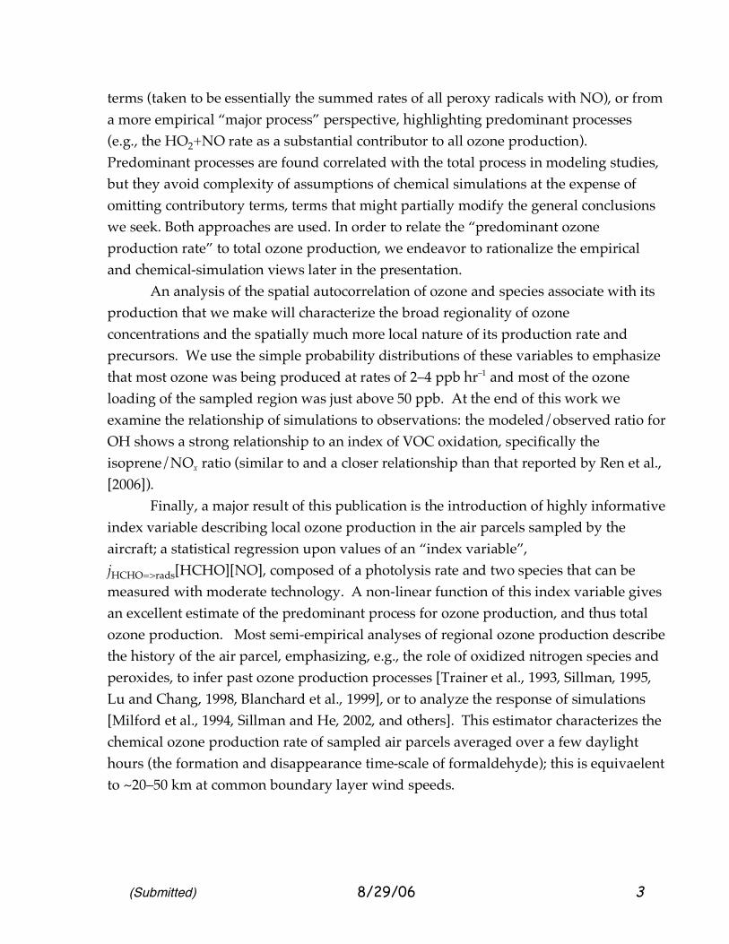
2. Results and Discussion 2.1 Context: Surface Ozone over Eastern North America The Environmental Protection Agency’s AIRNow reporting of tropospheric ozone for July 2004 gives a horizontal view at the surface. The month did not have great smog episodes characteristic of certain other years [Fuelberg et al., 2006]. However, the measurements shown in Figure 2 and on the AIRNOW website suggest that the period from July 20 through July 22 had relatively high ozone concentrations over fairly wide areas, with especially high values over the area east of the Appalachians on July 21 and July 22. This period exhibited relatively high ozone for summer, 2004, as an easy survey of all the AirNOW data will show. ___________________________________________________________

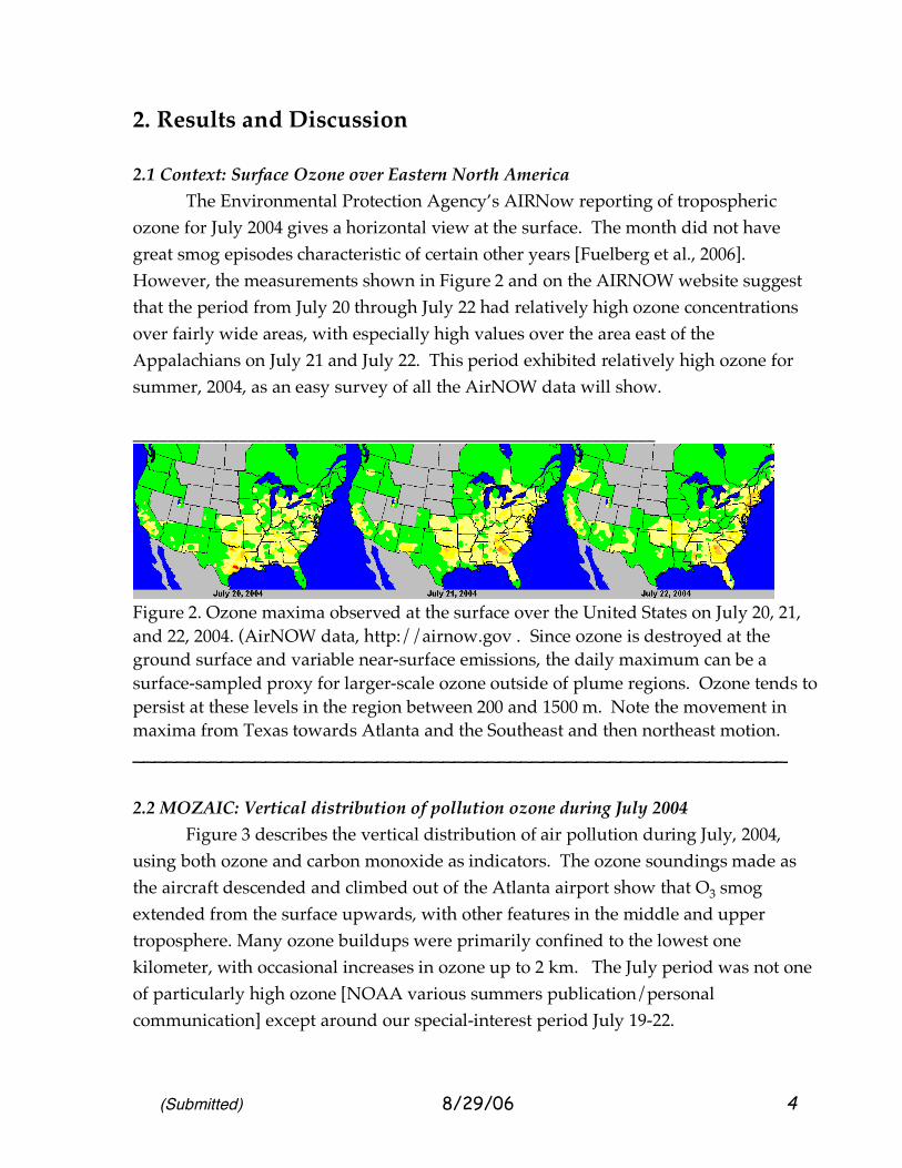
Figure 2. Ozone maxima observed at the surface over the United States on July 20, 21, and 22, 2004. (AirNOW data, http://airnow.gov . Since ozone is destroyed at the ground surface and variable near-surface emissions, the daily maximum can be a surface-sampled proxy for larger-scale ozone outside of plume regions. Ozone tends to persist at these levels in the region between 200 and 1500 m. Note the movement in maxima from Texas towards Atlanta and the Southeast and then northeast motion. ___________________________________________________________ 2.2 MOZAIC: Vertical distribution of pollution ozone during July 2004 Figure 3 describes the vertical distribution of air pollution during July, 2004, using both ozone and carbon monoxide as indicators. The ozone soundings made as the aircraft descended and climbed out of the Atlanta airport show that O3 smog extended from the surface upwards, with other features in the middle and upper troposphere. Many ozone buildups were primarily confined to the lowest one kilometer, with occasional increases in ozone up to 2 km. The July period was not one of particularly high ozone [NOAA various summers publication/personal communication] except around our special-interest period July 19-22.


The CO record provides a supplemental view: about origins of ozone in the troposphere. Commonly, CO reflects local pollution, particularly from cities (automobile emissions) but has a particularly strong response to biomass burning, local or distant. The CO shows similar confinement of pollution over the Southeast United States during the period, and extending frequently to ~ 2 km. A notable exception of the burning-influence period following July 20. The ozone pollution episode passing over the Atlanta area appears to be coincident or following another feature connected with the buildup of CO into the lower mid-troposphere. This view is compatible with the broad spatial characterization of a progressively subsiding smoke plume described in the next section. These observations at Atlanta bring up a long-standing question regarding the vertical extent of pollution, and a related question, the regionality of ozone pollution. Vertical extent and horizontal extent are related, given that air just above the boundary layer can move more rapidly and be less influenced by local effects, e.g. NO titration and surface deposition. Figure 3 suggests substantial similarity of atmospheric composition in the boundary layer up to 1 km or son with the composition up to 2.5–3 km. ___________________________________________________________

Figure 3. Ozone and carbon monoxide variations over the Southeast USA during July, as sampled by the MOZAIC instrumentation. Ozone maxima in the lower troposphere occur in the days around July 22 and August 4. High carbon monoxide concentrations in the lower troposphere suggest the degree of mixing of urban pollution in the upper troposphere, with the exception of the period around July 22, when subsidence of biomass burning pollution from Alaska into the area becomes apparent. Layers up to 2.5 km show similar types of ozone variation as the near-surface ozone. ___________________________________________________________


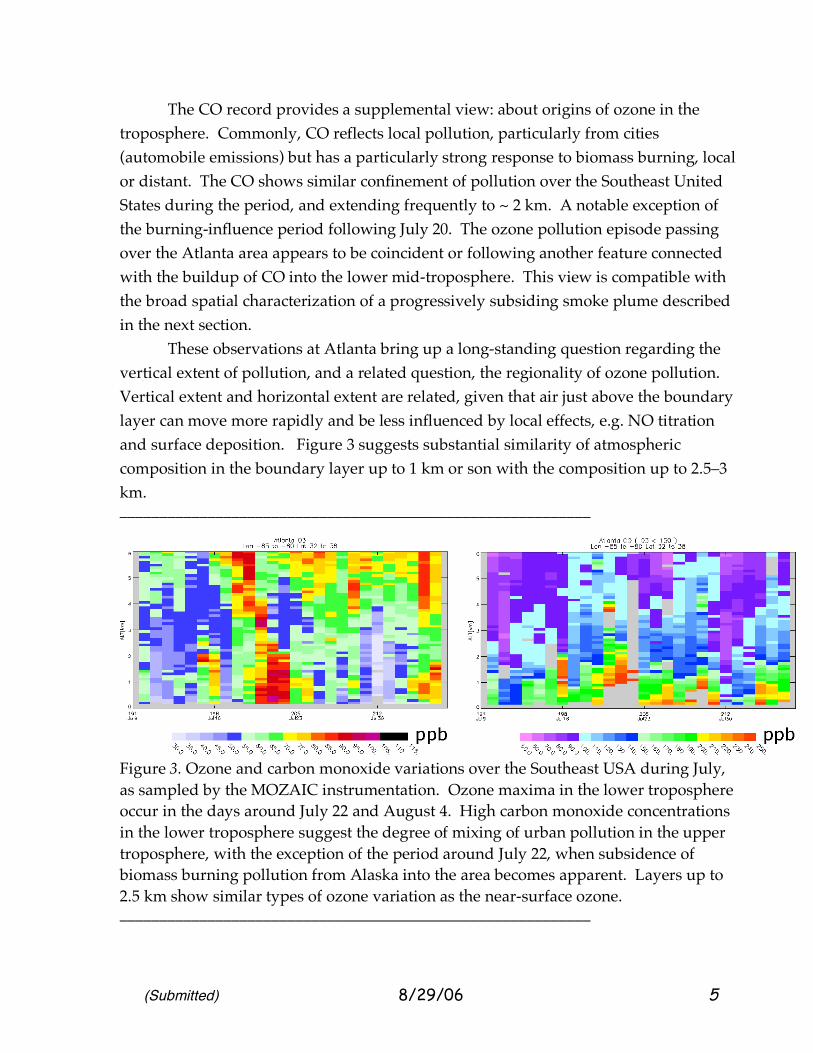
So far we have presented two views, a surface-measurement approximation of the smog-prone boundary layer and a vertical view at one point. In fact, tropospheric ozone has a rich variation in three dimensions, a variation that needs to be characterized and whose simulations must be checked in greater detail. 2.3 A Broad Depiction of Lower Tropospheric Smog Ozone: July 20, 2004. On Flight 10, the DC-8 created a sketch view of the vertical and horizontal distribution of ozone over Eastern North America on July 20, 2004, early in the smog-buildup period. Differential Absorption Lidar (DIAL) measurements [Al-Saadi et al., 2006] of ozone provided a view throughout the troposphere and into the lower stratosphere along the flight-path of the DC-8 aircraft. Since lidar sampling is impractical in the immediate ~500 m above and below the aircraft, ozone is interpolated through that region, but with use of the sample available from the Avery on-board instrument [Browell et al., 2006]. Figure 4 provides a schematic description of ozone over the Eastern United States. There is also a depiction of the DIAL reports of aerosol backscatter. These small aerosol particles provide a “pollution” description with some commonality to the MOZAIC descriptions of CO. There are also differences. CO and aerosol both indicate upwind forest or biomass burning very strongly, but CO also tends to respond to urban pollution (automobiles), while the aerosol backscatter responds to a variety of particulate sources, including sulfate aerosol (coal burning), organic aerosol (various combustion, urban and natural sources), and dust. In these samples, the black colors at elevated altitudes tend to correspond to smoke influence. Figures 4 (a and b) provide a highly graphic view of the variability of ozone on the cross-country flight of July 20. There is some smoothing of these profiles to maintain a consistent level of accuracy; for this reason a strong decrease in ozone within the first ~15–30 m, the surface layer [Davis, 1992, Kurpuis and Goldstein, 2005] is not seen. Local emissions and surface-layer ozone reaction are thought to influence surface monitoring sites. Correlation of the high ozone regions with location suggested that high ozone was not necessarily found directly over cities; a variety of downwind plumes were seen. Note also that similar patterns of ozone were found in the region below 1 km (roughly the daytime boundary layer) and the region directly above, 1-2.5 km. This suggests that the regions are connected with similar ozone chemistry, the upper layer of course likely to be lower in precursors, but also more removed from surface deposition, reaction with fresh nitric oxide and highly reactive alkenes (e.g., terpenes). We speculate that the similarity arises from the frequent exchange of ozone and its precursors by cloud venting, and by passage over areas where the boundary


layer is locally somewhat deeper due to strong heat fluxes from the surface or elevated terrain. These observations support the potential importance of lower tropospheric ozone on the phytotoxic ozone of pollution concern near the surface. ___________________________________________________________


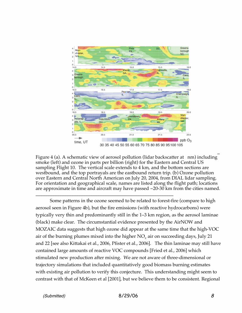
_ Figure 4 (a). A schematic view of aerosol pollution (lidar backscatter at nm) including smoke (left) and ozone in parts per billion (right) for the Eastern and Central US sampling Flight 10. The vertical scale extends to 4 km, and the bottom sections are westbound, and the top portrayals are the eastbound return trip. (b) Ozone pollution over Eastern and Central North American on July 20, 2004, from DIAL lidar sampling. For orientation and geographical scale, names are listed along the flight path; locations are approximate in time and aircraft may have passed ~20-30 km from the cities named. __________________________________________________________ Some patterns in the ozone seemed to be related to forest-fire (compare to high aerosol seen in Figure 4b), but the fire emissions (with reactive hydrocarbons) were typically very thin and predominantly still in the 1–3 km region, as the aerosol laminae (black) make clear. The circumstantial evidence presented by the AirNOW and MOZAIC data suggests that high ozone did appear at the same time that the high-VOC air of the burning plumes mixed into the higher NOx air on succeeding days, July 21 and 22 [see also Kittakai et al., 2006, Pfister et al., 2006]. The thin laminae may still have contained large amounts of reactive VOC compounds [Fried et al., 2006] which stimulated new production after mixing. We are not aware of three-dimensional or trajectory simulations that included quantitatively good biomass burning estimates with existing air pollution to verify this conjecture. This understanding might seem to contrast with that of McKeen et al [2001], but we believe them to be consistent. Regional


simulations suggest that most of the high ozone in the southern US portion of the sampling was associated with an eastward-moving regional sulfate episode [Carmichael et al., 2006].

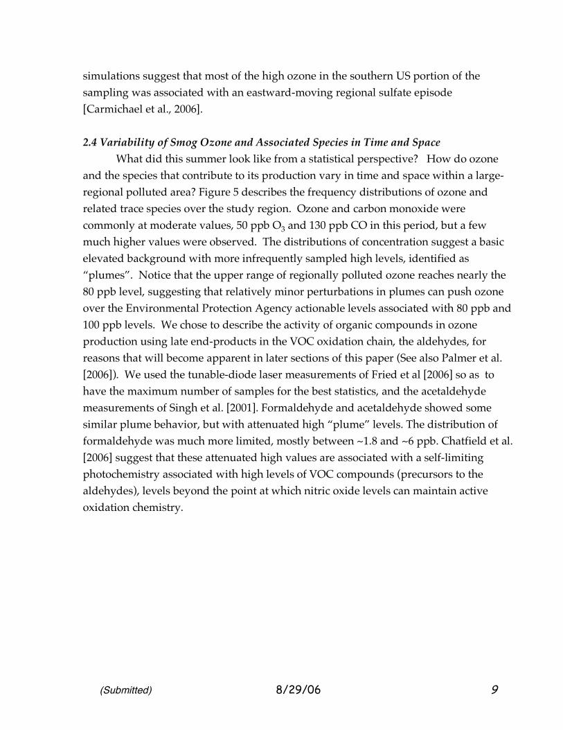
2.4 Variability of Smog Ozone and Associated Species in Time and Space What did this summer look like from a statistical perspective? How do ozone and the species that contribute to its production vary in time and space within a large-regional polluted area? Figure 5 describes the frequency distributions of ozone and related trace species over the study region. Ozone and carbon monoxide were commonly at moderate values, 50 ppb O3 and 130 ppb CO in this period, but a few much higher values were observed. The distributions of concentration suggest a basic elevated background with more infrequently sampled high levels, identified as “plumes”. Notice that the upper range of regionally polluted ozone reaches nearly the 80 ppb level, suggesting that relatively minor perturbations in plumes can push ozone over the Environmental Protection Agency actionable levels associated with 80 ppb and 100 ppb levels. We chose to describe the activity of organic compounds in ozone production using late end-products in the VOC oxidation chain, the aldehydes, for reasons that will become apparent in later sections of this paper (See also Palmer et al. [2006]). We used the tunable-diode laser measurements of Fried et al [2006] so as to have the maximum number of samples for the best statistics, and the acetaldehyde measurements of Singh et al. [2001]. Formaldehyde and acetaldehyde showed some similar plume behavior, but with attenuated high “plume” levels. The distribution of formaldehyde was much more limited, mostly between ~1.8 and ~6 ppb. Chatfield et al. [2006] suggest that these attenuated high values are associated with a self-limiting photochemistry associated with high levels of VOC compounds (precursors to the aldehydes), levels beyond the point at which nitric oxide levels can maintain active oxidation chemistry.


___________________________________________________________

Figure 5. Observed values of ozone and related species as sampled in the boundary layer over the Central United States in July-August, 2004. Statistics describe all air parcels sampled 0–1300 m ASL. “Violin plots” describe a smoothed estimate of probability distribution of the species. (a) Ozone and CO (ppb) display sharp “plume” high concentrations above a basic regional elevated level in these non-logarithmic plots. (These ozone measurements were sampled on board the DC-8.) Aldehyde concentrations (ppb) display somewhat attenuated plume peaks. (b) Log concentration plots of nitric oxide, the active nitrogen oxides NOx, HO2 and OH, in pptv. NO is a primary emission, and NO and NOx show extreme peaks. The central photochemical radicals, HO2 and OH, like formaldehyde, show attenuated “plume” or peak concentrations. NO concentrations become increasingly uncertain below 20 ppt. ___________________________________________________________ In contrast to the organics, the conjugate ozone precursor, nitric oxide ranged much more widely, requiring a logarithmic scale to describe their probability distribution. The associated “active nitrogen oxides” NOx = NO + NO2: many observations of NOx were near 50 ppt, and many near 4000–7000 ppt, and some going over 25000 ppt, i.e. 100 to 500 times as high in concentration. No self-limiting behavior is observed for these species: NO (see Ren et al. [2006]) is a direct emission and high concentrations result without photochemistry and NO2 is produced readily. (Nitric oxide measurements were regarded as increasingly unreliable below 20, even 50 ppt, but show a smooth distribution down to at least 5 ppt. Samples with low concentrations were kept in the analysis because measures such as ozone production were minimally affected by uncertainties in low concentrations, and removing the low-NO cases would create greater distortions.) (The distributions shown suggest that the


lowest ~5–10% of concentrations, associated with non-smoggy air, must be considered cautiously. In fact, we set an arbitrary minimum for NO concentrations of 10 ppt.) NO2 measurements were from the Berkeley group [Bertram et al., 2006]. Nevertheless, distributions measured on reported NO and NOx display anomalies at low concentrations; these are small effects describing sample of non-smog over Eastern North America or immediately downwind. Aside from these features, the symmetric distribution of the nitrogen species, approximating log-normal, invites further exploration. ___________________________________________________________

Figure 6. Widely differing smog-production conditions as sampled in the continental boundary layer ozone by the NASA DC-8 during INTEX-NA. Color scale refers to log10 of the “formaldehyde activity” divided by the NOx concentration, in ppt units. Formaldehyde activity is taken to be the formaldehyde concentration times its photolysis rate (s-1) to radicals and CO, and is described below to be one measure of VOC weighted by reactivity. Approximately 1800 samples over the populated regions of Central and Eastern North America were included, or samples potentially just downwind. Altitudes up to 1300 m ASL were included since the DIAL observations suggested that they were relatively similar in ozone and aerosol characteristics, e.g., influenced by cloud mixing. The significance of these quantities in describing ozone production will be described later in the paper and in Chatfield et al. [2006]. We conclude that a wide variety of NOx-limited and VOC- (radical-production-) limited areas were sampled. ___________________________________________________________


Figure 5 also describes the observed distribution of the central photochemical species OH and HO2. In log-normal terms, these also display attenuated high values or “plume” structures. Chatfield et al [2006] considers these self-limiting “high pollution” effects, which may be associated with either high VOC or high NOx. The nitrogen oxides and VOC compounds (and hence formaldehyde) often vary quite independently, as the map Figure B6 shows. But what causes ozone to rise to the levels observed in this moderate regional smog? There are two approaches to describing the production of ozone, each with its advantages; we present both. The level of smog ozone in a region is usefully described by a linearized equation that simplifies all the interacting cross-reactions of the smog process.

d [O3] / dt = P O3 – L O3

[O3] – D O3 + T O33

where P , D, and T describe the chemical production rate of ozone, the deposition to the surface and the complex term describing transport, sometimes positive, sometimes negative. These have units of molec.cm–3s–1 or ppb. L is a chemical loss rate of ozone and has the units of s–1, or more conveniently day–1 . These terms are distributed statistically in patterns that are characteristically different from the ozone concentration itself, which integrates effects over space and time. One good way to estimate these terms is through the use of a chemical model that includes much of the complex reaction chemistry. It is possible to provide a reasonable estimate based on the species measured by the DC-8. Important species are NOx = NO + NO2, O3 itself, volatile organic carbon species which can be measured, peroxy acetyl nitrate, water, photlysis rates, etc. We use results of a “point” chemical model using the smog-chemistry mechanism and the required simplifying “point”-model assumptions provided for the INTEX-NA period [Olson, et al, 2006]. Other reaction mechanisms are arguably more complete descriptions of the chemistry. However, we note that this model must make assumptions about reactive intermediates that are not measurable. Specifically, the model results assume a repeating set of initial-emission concentrations continuing unchanged in time, and chosen to be those measured aboard the aircraft. Where available, hydrogen peroxide, methyl peroxide, peroxy acetyl nitrate, nitric acid were used as constraints; in relatively few cases they were calculated. Measured volatile organic compounds, including hydrocarbons, methanol and acetone, were used when simultaneous measurements were available, otherwise they were interpolated. Observed photolysis rates were used [Shetter and Muller, 1999]. The results shown have UV radiation appropriate to the (daylight)


measurement aboard the DC-8, but the integration reflects an implicit 24-hour cycle. Ren et al. [2006] have more discussion of the point-model values and corresponding observations. Three-dimensional models can usefully add effects transport, particularly the effects of previous high values (chemical decay). However for chemical estimation like this, they also complicate chemical analyses with uncertainties of sources and transport simulation. The calculations are useful, and show behavior consistent generally with a more empirical “major terms” analysis described below. Comparisons of OH, HO2, and their ratio are made at the conclusion of the paper. Figure 7 shows the results of these calculations. We portray ozone chemical production, ozone loss LossO3 = L O3

[O3], net ozone chemical ozone production minus loss, and the timescale associated with ozone loss (L O3

–1 ). The ozone loss described by the point model includes most common free-tropospheric processes, but does not include, e.g., reaction with complex, very reactive terpenes, e.g., the pinenes. Surface reaction or “deposition” was not included either. These reactions probably occur very near the surface, away from the DC-8 sampling, and are better described by other techniques concentrating on surface sites [Davis, 1992, Tan et al., 2001, Kurpuis and Goldstein, 2005,]. Titration of ozone by fresh NO, e.g. from power plants, is also omitted. Temporary transfer of the oxidizing power from O3 to NO2 may be considered inappropriate to this scaling analysis; we admit that careful consideration of the fate of NO2 is appropriate for more quantitative budget analyses. This work concentrates on mid-boundary-layer terms that are otherwise difficult to sample. Figure 8 gives a different perspective on the distribution of pollutants. To answer the question: “the average pollution loading is due mostly to just which concentration ranges?” we need a plot different from ordinary probability or histogram plts. Figure 8 shows the probability weighted instances of various concentrations: i.e., the area of the figure represents the average concentration, and large areas within the distribution describe which concentration ranges account for most of the total pollutant loading observed during all the INTEX-NA flights. Notice the importance of ~50–60 ppb ozone regions to the total ozone loading over the Eastern/Central United States during this period. Notice also the significance of regions producing only 1.5–4 ppb/hour of ozone to ozone production in the sampled area. Analysis not displayed suggests that most ozone creation in our sample took place at 40–50 ppb levels of ozone. This appears consistent with the idea that strong plume production processes can produce locally very high ozone production rate and ozone values. However, most ozone is produced more regionally at a few ppb/hour, and we suggest that this raises the level of ozone so as eventually to the pass levels exceeding Federal standards.


___________________________________________________________

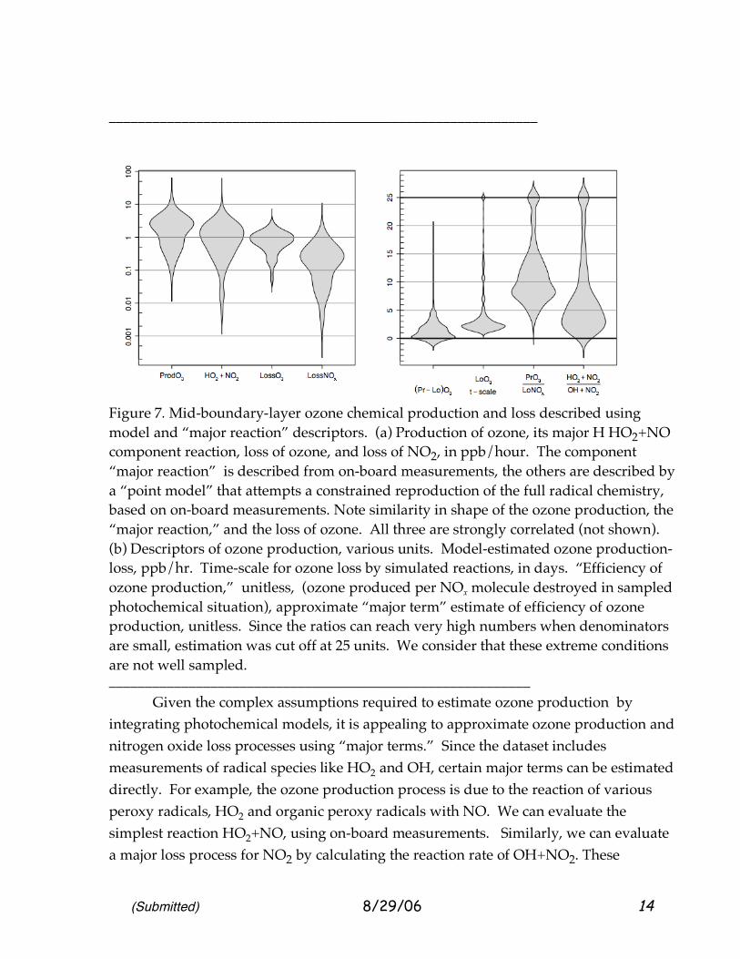
Figure 7. Mid-boundary-layer ozone chemical production and loss described using model and “major reaction” descriptors. (a) Production of ozone, its major H HO2+NO component reaction, loss of ozone, and loss of NO2, in ppb/hour. The component “major reaction” is described from on-board measurements, the others are described by a “point model” that attempts a constrained reproduction of the full radical chemistry, based on on-board measurements. Note similarity in shape of the ozone production, the “major reaction,” and the loss of ozone. All three are strongly correlated (not shown). (b) Descriptors of ozone production, various units. Model-estimated ozone production-loss, ppb/hr. Time-scale for ozone loss by simulated reactions, in days. “Efficiency of ozone production,” unitless, (ozone produced per NOx molecule destroyed in sampled photochemical situation), approximate “major term” estimate of efficiency of ozone production, unitless. Since the ratios can reach very high numbers when denominators are small, estimation was cut off at 25 units. We consider that these extreme conditions are not well sampled. __________________________________________________________ Given the complex assumptions required to estimate ozone production by integrating photochemical models, it is appealing to approximate ozone production and nitrogen oxide loss processes using “major terms.” Since the dataset includes measurements of radical species like HO2 and OH, certain major terms can be estimated directly. For example, the ozone production process is due to the reaction of various peroxy radicals, HO2 and organic peroxy radicals with NO. We can evaluate the simplest reaction HO2+NO, using on-board measurements. Similarly, we can evaluate a major loss process for NO2 by calculating the reaction rate of OH+NO2. These


processes often account for > 60% of ozone production and NOx loss, and so serve as excellent, more observation-based indicators of ozone production and NOx loss. We will refer to the HO2+NO rate as the “predominant ozone production rate.” Therefore Figure 7 also portrays observed distributions of these “major term” quantities. _________________________________________________________

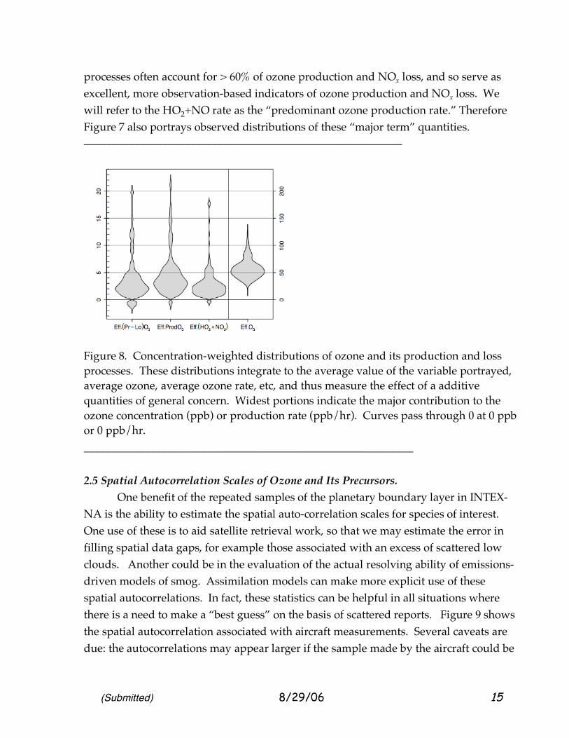
Figure 8. Concentration-weighted distributions of ozone and its production and loss processes. These distributions integrate to the average value of the variable portrayed, average ozone, average ozone rate, etc, and thus measure the effect of a additive quantities of general concern. Widest portions indicate the major contribution to the ozone concentration (ppb) or production rate (ppb/hr). Curves pass through 0 at 0 ppb or 0 ppb/hr. ___________________________________________________________ 2.5 Spatial Autocorrelation Scales of Ozone and Its Precursors. One benefit of the repeated samples of the planetary boundary layer in INTEX-NA is the ability to estimate the spatial auto-correlation scales for species of interest. One use of these is to aid satellite retrieval work, so that we may estimate the error in filling spatial data gaps, for example those associated with an excess of scattered low clouds. Another could be in the evaluation of the actual resolving ability of emissions-driven models of smog. Assimilation models can make more explicit use of these spatial autocorrelations. In fact, these statistics can be helpful in all situations where there is a need to make a “best guess” on the basis of scattered reports. Figure 9 shows the spatial autocorrelation associated with aircraft measurements. Several caveats are due: the autocorrelations may appear larger if the sample made by the aircraft could be


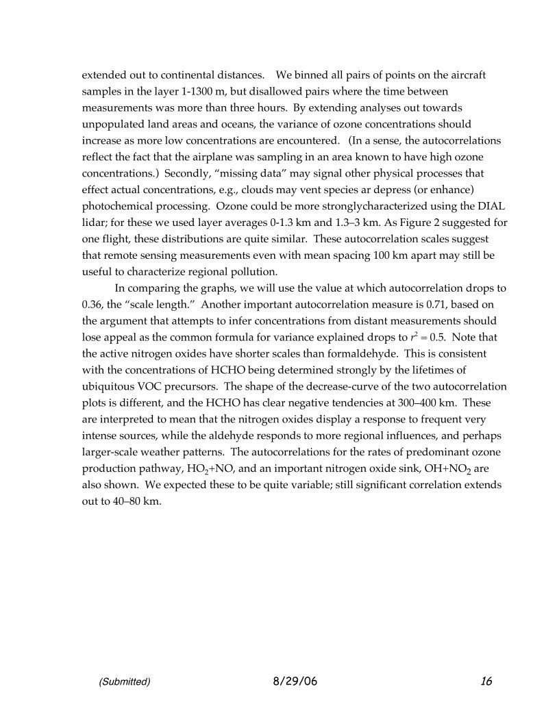
extended out to continental distances. We binned all pairs of points on the aircraft samples in the layer 1-1300 m, but disallowed pairs where the time between measurements was more than three hours. By extending analyses out towards unpopulated land areas and oceans, the variance of ozone concentrations should increase as more low concentrations are encountered. (In a sense, the autocorrelations reflect the fact that the airplane was sampling in an area known to have high ozone concentrations.) Secondly, “missing data” may signal other physical processes that effect actual concentrations, e.g., clouds may vent species ar depress (or enhance) photochemical processing. Ozone could be more stronglycharacterized using the DIAL lidar; for these we used layer averages 0-1.3 km and 1.3–3 km. As Figure 2 suggested for one flight, these distributions are quite similar. These autocorrelation scales suggest that remote sensing measurements even with mean spacing 100 km apart may still be useful to characterize regional pollution. In comparing the graphs, we will use the value at which autocorrelation drops to 0.36, the “scale length.” Another important autocorrelation measure is 0.71, based on the argument that attempts to infer concentrations from distant measurements should lose appeal as the common formula for variance explained drops to r2 = 0.5. Note that the active nitrogen oxides have shorter scales than formaldehyde. This is consistent with the concentrations of HCHO being determined strongly by the lifetimes of ubiquitous VOC precursors. The shape of the decrease-curve of the two autocorrelation plots is different, and the HCHO has clear negative tendencies at 300–400 km. These are interpreted to mean that the nitrogen oxides display a response to frequent very intense sources, while the aldehyde responds to more regional influences, and perhaps larger-scale weather patterns. The autocorrelations for the rates of predominant ozone production pathway, HO2+NO, and an important nitrogen oxide sink, OH+NO2 are also shown. We expected these to be quite variable; still significant correlation extends out to 40–80 km.


_________________________________________________________


Figure 9. Spatial autocorrelation of ozone and associated variables from the INTEX-NA flights. Ozone autocorrelations may be calculated for all pairs of DIAL points measured within three hours of each other. The first two diagrams describe ~3000 points per distance bin. Average ozone mixing ratios are calculated for layers 0 to 1.3 km and 1.3 km to 3 km, regions which may be resolvable by remotely sensed data. The related species are calculated from the any on-board measurements made between 0 and 1.3 km. Two trends are apparent. Ozone has much longer autocorrelation spatial scales than its precursor and source-associated variables, and the autocorrelation spatial scale increases slowly with altitude. Formaldehyde, the active nitrogen oxides, and rates related to ozone production and NOx loss have behavior consonant with the sources of ozone precursors, VOC and NO. __________________________________________________________ 2.6 An Index Variable Quantifying Local Ozone Production The relatively complete atmospheric sampling we report allows an exploration and validation of a minimal informative set of measurements that allow evaluation important environmental quantities like the local ozone production rate. By analogy with a common term in economic data analysis, we assert that there may be “index variable” that allows a very informative determination of the local ozone production rate. An index variable provides enough basic information to predict important quantities without the need for all information that might at first seem necessary. We use the term to imply a remarkable but not complete correlation with, e.g., the local ozone production rate. Photochemical smog is notoriously complex; consequently we expand somewhat and test estimators of the local ozone production rate elsewhere [Chatfield et al., 2006]. We advance our choice with a combination of physical and statistical arguments, recognizing the limits of each.


_________________________________________________________

a

b c

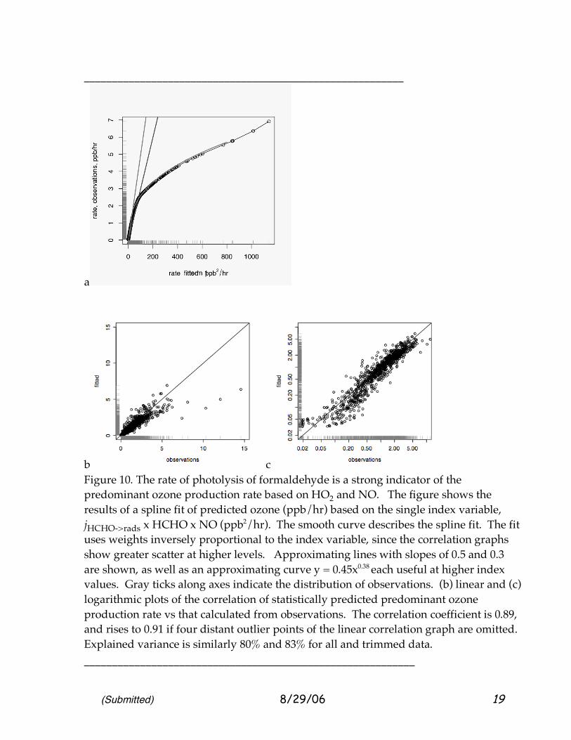
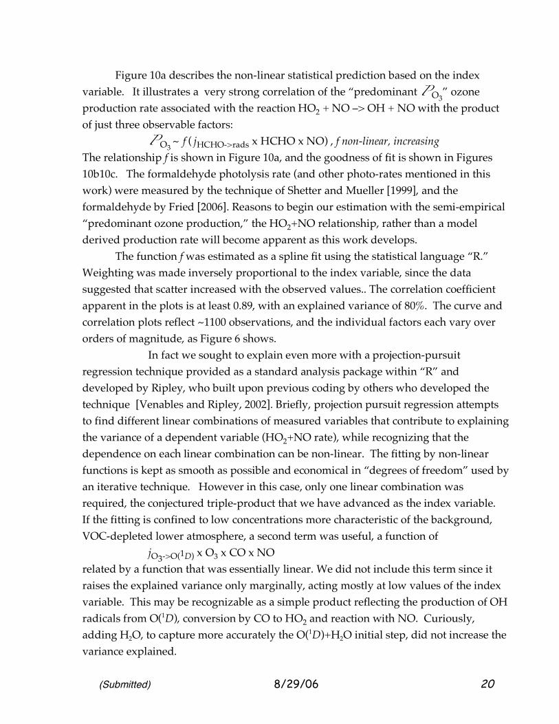
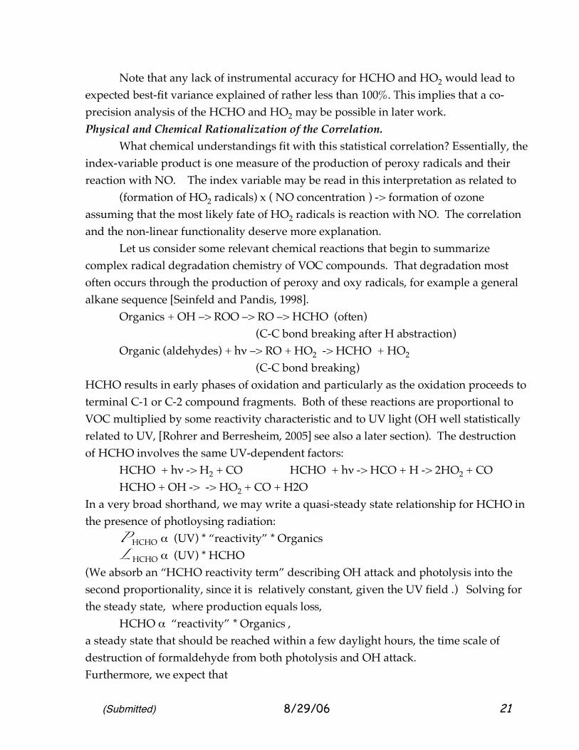
Figure 10. The rate of photolysis of formaldehyde is a strong indicator of the predominant ozone production rate based on HO2 and NO. The figure shows the results of a spline fit of predicted ozone (ppb/hr) based on the single index variable, jHCHO->rads x HCHO x NO (ppb2/hr). The smooth curve describes the spline fit. The fit uses weights inversely proportional to the index variable, since the correlation graphs show greater scatter at higher levels. Approximating lines with slopes of 0.5 and 0.3 are shown, as well as an approximating curve y = 0.45x0.38 each useful at higher index values. Gray ticks along axes indicate the distribution of observations. (b) linear and (c) logarithmic plots of the correlation of statistically predicted predominant ozone production rate vs that calculated from observations. The correlation coefficient is 0.89, and rises to 0.91 if four distant outlier points of the linear correlation graph are omitted. Explained variance is similarly 80% and 83% for all and trimmed data. ___________________________________________________________


Figure 10a describes the non-linear statistical prediction based on the index variable. It illustrates a very strong correlation of the “predominant P O3

” ozone production rate associated with the reaction HO2 + NO –> OH + NO with the product of just three observable factors: P O3

~ f (

jHCHO->rads x HCHO x NO) , f non-linear, increasing

The relationship f is shown in Figure 10a, and the goodness of fit is shown in Figures 10b10c. The formaldehyde photolysis rate (and other photo-rates mentioned in this work) were measured by the technique of Shetter and Mueller [1999], and the formaldehyde by Fried [2006]. Reasons to begin our estimation with the semi-empirical “predominant ozone production,” the HO2+NO relationship, rather than a model derived production rate will become apparent as this work develops. The function f was estimated as a spline fit using the statistical language “R.” Weighting was made inversely proportional to the index variable, since the data suggested that scatter increased with the observed values.. The correlation coefficient apparent in the plots is at least 0.89, with an explained variance of 80%. The curve and correlation plots reflect ~1100 observations, and the individual factors each vary over orders of magnitude, as Figure 6 shows. In fact we sought to explain even more with a projection-pursuit regression technique provided as a standard analysis package within “R” and developed by Ripley, who built upon previous coding by others who developed the technique [Venables and Ripley, 2002]. Briefly, projection pursuit regression attempts to find different linear combinations of measured variables that contribute to explaining the variance of a dependent variable (HO2+NO rate), while recognizing that the dependence on each linear combination can be non-linear. The fitting by non-linear functions is kept as smooth as possible and economical in “degrees of freedom” used by an iterative technique. However in this case, only one linear combination was required, the conjectured triple-product that we have advanced as the index variable. If the fitting is confined to low concentrations more characteristic of the background, VOC-depleted lower atmosphere, a second term was useful, a function of jO3->O(1D) x O3 x CO x NO related by a function that was essentially linear. We did not include this term since it raises the explained variance only marginally, acting mostly at low values of the index variable. This may be recognizable as a simple product reflecting the production of OH radicals from O(1D), conversion by CO to HO2 and reaction with NO. Curiously, adding H2O, to capture more accurately the O(1D)+H2O initial step, did not increase the variance explained.


Note that any lack of instrumental accuracy for HCHO and HO2 would lead to expected best-fit variance explained of rather less than 100%. This implies that a co-precision analysis of the HCHO and HO2 may be possible in later work. Physical and Chemical Rationalization of the Correlation. What chemical understandings fit with this statistical correlation? Essentially, the index-variable product is one measure of the production of peroxy radicals and their reaction with NO. The index variable may be read in this interpretation as related to (formation of HO2 radicals) x ( NO concentration ) -> formation of ozone assuming that the most likely fate of HO2 radicals is reaction with NO. The correlation and the non-linear functionality deserve more explanation. Let us consider some relevant chemical reactions that begin to summarize complex radical degradation chemistry of VOC compounds. That degradation most often occurs through the production of peroxy and oxy radicals, for example a general alkane sequence [Seinfeld and Pandis, 1998]. Organics + OH –> ROO –> RO –> HCHO (often) (C-C bond breaking after H abstraction) Organic (aldehydes) + hν –> RO + HO2 -> HCHO + HO2 (C-C bond breaking) HCHO results in early phases of oxidation and particularly as the oxidation proceeds to terminal C-1 or C-2 compound fragments. Both of these reactions are proportional to VOC multiplied by some reactivity characteristic and to UV light (OH well statistically related to UV, [Rohrer and Berresheim, 2005] see also a later section). The destruction of HCHO involves the same UV-dependent factors: HCHO + hν -> H2 + CO HCHO + hν -> HCO + H -> 2HO2 + CO HCHO + OH -> -> HO2 + CO + H2O In a very broad shorthand, we may write a quasi-steady state relationship for HCHO in the presence of photloysing radiation: P HCHO α (UV) * “reactivity” * Organics L HCHO α (UV) * HCHO (We absorb an “HCHO reactivity term” describing OH attack and photolysis into the second proportionality, since it is relatively constant, given the UV field .) Solving for the steady state, where production equals loss, HCHO α “reactivity” * Organics , a steady state that should be reached within a few daylight hours, the time scale of destruction of formaldehyde from both photolysis and OH attack. Furthermore, we expect that


P HO2 α (UV) * HCHO since all sources of HO2 (photolysis of aldehydes, alkoxy radical H-abstraction, etc) involve P HO2 α (UV) * “reactivity” * Organics L HO2 α g NO + h( HO2) + smaller terms, g linear, h increasing, non-linear (smaller terms describe reaction with O3, HO2; more discussion below). It is then reasonable that the principal production rate of ozone be approximated Principal Production = f( k (UV) * [HCHO] * “reactivity” * [Organics] * [NO] ) Furthermore, reactions producing alkyl peroxy and acyl peroxy radicals are highly correlated with these same factors, since these reactions occur within fractions of a second to hours before and after HO2 production involving aldehydes: Other Production = f’o( k (UV) * [HCHO] * “reactivity” * [Organics] * [NO] ) Summarizing to this point, jHCHO->rads x HCHO is an indicator of reaction chemistry producing radicals since all photolytic reactions (and OH radical concentrations) tend to be related, and HCHO is a reasonable indicator of VOC oxidation or processing. For this reason, we describe jHCHO->rads x HCHO as a “gauge” measuring the rate of much larger set of chemical processes as they produce ozone. The relationship f is not linear. Approximate loss terms for HO2 depending on NO and HO2 were mentioned above). More generally, note that as the production rate or radicals goes up, various kinds of termination reactions for HO2 and OH occur. For example, HO2 + HO2 -> H2O2-> deposition or -> OH + OH (peroxide photolysis) ROO + HO2 -> ROOH + O2 OH + NO2 -> HNO3 -> deposition or -> OH + HNO3 -> H2O + NO3 (The latter reaction becomes prominent as both radical production and NOx levels rise; the former are more important at moderate radical production rates and low NOx.) In the simplest analysis, the function f should rise linearly from zero as radicals begin to be formed, and then should flatten into an approximate square-root behavior. Figure 10a indicates straight lines passing through zero with slopes of 0.03 and 0.05, respectively. An approximate square-root dependence might be expected where the HO2 + HO2

provides the main sink for HO2, but that a small amount of HO2 instead reacts with NO to make ozone. The figure sketches in a similar dependence curve, with an estimated 0.38 power rather than a 0.5 power. Beyond this simple description, smog radical chemistry becomes extremely complex, and so we rely on statistical regression relationships to estimate the “fall-off” relationship involved with radical-radical self reactions and other limiting aspects of photochemical smog ozone production. This is


exactly the behavior of the statistical fit. We note that the fitted function makes changes of slope for the few highest cases with production above 5 ppb/hr, and that these are need much better empirical determination. At the very lowest levels, where all variables may have measurement difficulties, there appears to be one linear trend, above that the linear trend seems lower. Of more interest is the kink where the abscissa is ~15. Perhaps other, broadly sampled, data could suggest a smoother curve; little effect on the predictive capability would be expected. The economy of the curve fit for ~1100 samples is excellent. Whereas a curve like y = a xb involves 3–4 degrees of freedom and a piece-by-piece curve several more, the “equivalent degrees of freedom” providing the common description of the empirical spline fit gives an edf = 5.3 [Venables and Ripley, 2003]. (A parabolic fit (df = 3) with e very slight curve would have edf closer to 2 than 3.) Figure 10 should also be interpreted carefully for two reasons. First, the plot is clearly one of a[NO] vs b(an increasing function of [NO]), and so inherently tends to be correlated. Second, the expression kHO2NO[HO2][NO] represents only a major portion of ozone production, not all production of ozone, especially those involving organic peroxy radicals and peroxy acyl radicals. Let us consider each of these important caveats. Figure 10 certainly contains the common factor [NO] in abscissa and the ordinate. However, [NO] is required to obtain the desired quantity, ozone production, and hence yields an impression of the accuracy of our estimate. The very strong role of [NO] in determining ozone production has been evident for years [Crutzen, 1972, Chameides et al., 1992, Liu, et al., 1987] and the “common factor” emphasizes that one simply must include [NO] in the formula. This is not the only reason for the excellent relationship, however, A linear relationship of the HO2+NO rate with [NO] does hold, but the correlation plot is a broad, widening triangle, and the explained variance is only 40%; i.e., more precise information is available when we add the formaldehyde-related factors. Chatfield et al [2006] describe a two-parameter approach also; this raises the variance explained to perhaps 96%, with the same points being apparent outliers. The one-parameter and the two-parameter fits each have their value in describing ozone formation. 2.7 Predominant and Total Estimates of Ozone Formation. The second consideration, the “predominant ozone formation rate” and our best estimate of the true rate, requires us to move from direct indicators of ozone production to simulation: measurement of all peroxy radicals was not made on the DC-8; those


measurements would allow a very close estimate of total oxidant production. Use of a peroxy radical estimator like PERCA [Cantrell et al., 1996] might raise questions on how we relate the PERCA chamber measurement environment to the environments characterizing natural atmospheric parcels with a large variation of chemical conditions, but could be interesting future research. _________________________________________________________

Figure 11. (a) Relationship of several measures of ozone production. The principal rate is taken to be the rate of reactions of HO2 radicals with NO, in ppb/hour. The x axis shows that rate based on the Langley model, in which both NO and HO2 are simulated. The gray circles plot the observed value of the rate plotted for corresponding points. The light gray line indicates a simple linear fit. See a later section for further comparisons, especially of HO2. The black dots relate the principal ozone production term to the Langley model estimate of ozone production. Lines of slope 1, 2, and 3 are drawn, as well as the regression line. The regression line has slope ~ 1.57 and intercept .02, with a R2 of 0.91. (b) A q-q plot of modeled (abcissa) and observed (ordinate) quantiles of kHO2NO[HO2][NO] “principle production rate.” Compare this near straight-line to the behavior of OH and HO2 (Note: these axes are flipped from our standard practice.). __________________________________________________________ An optimistic view of the chemical inter-relationships described by the point-model fit is this. Each set, observed and model-derived, is self-consistent set of chemically reacting species (to the extent the model is capable of expressing current rate-coefficient knowledge), a parallel set of concentrations following, to the best of our knowledge, the same laws. Interpolation and difficulties associated with simultaneous measurement should leave the model reaction-species set nevertheless very close to the observed set, even if point comparisons vary. Figure 11 places the computed values of the predominant ozone production pathway on the abscissa (contrary to our usual


practice). The points in gray a comparison of the modeled to observed kHO2NO[HO2][NO]. The scatter is large, and might point to interpolation difficulties. For the current purposes, we note that a q-q plot of the quantiles of observed and simulated kHO2NO[HO2][NO] follow the 1:1 line fairly well, but most of the highest 2% of simulated rates do not reach quite high values as observed. The simple regression line might probably be close to 1:1 but for these influential high points. A later section will describe the evidence that there are greater difficulties with the HOx budget than this optimistic interpretation of the q-q plot suggests. For whatever reasons, the estimation of “predominant ozone production rate” remains less affected by uncertainties. The black dots and dark gray regression line suggest that the relationship of the “predominant ozone formation rate” and the total formation rate is indeed very close, for the model. A regression analysis a multiplier of approximately 1.6 can be used to estimate complete ozone production: Complete P(O3) = (1.57+0.2)• kHO2NO[HO2][NO] + (0.3+.03) The results are quite significant: R2 = 0.91, although we consider that there may be considerable uncertainty attached to the use of any chemical reaction mechanism. A statistical analysis seeking to fit ozone production to the index variable and also other factors suggest that variance explained R2 can be increased to > 98% by adding a measurement of acetaldehyde to the fitting procedure, but this improvement may be very dependent on the nature of the chemical reaction mechanism used. Chatfield et al [2006] describe considerations in more detail. We note that the simulation of acetaldehyde in the lower troposphere exhibits both under-estimation and over-estimation of the species, so that the statistical relationships found in the model must be carefully re-examined as our knowledge of organic oxidation improves. The technique used to establish this was once again projection pursuit regression, but in this case both the modeled HO2+NO rate and acetaldehyde concentrations were found necessary to raise the explained variance to a satisfactory level. This mix of chemical modeling and observational “predominant ozone production rate” analysis is complex. However, model estimation of the total-to-predominant (ROO+HO2 to HO2-only) ozone production process remains the estimation procedure that is currently practical, since estimation of total chemical ozone production uninfluenced by transport considerations is quite elusive. In summary, we have found from a largely empirical analysis that the predominant ozone production rate, HO2+NO, has a single, non-linear dependence on an index variable, jHCHO->rads x HCHO x NO, through a non-linear but increasing


function. The relationship holds for an extremely wide range of concentrations measured in the lowest 1.5 km during INTEX-NA. Since we have no simple measurement of total ozone production rate from all peroxy radicals, we have used a self-consistent photochemical model to estimate the relationship of the predominant and total rates. Since all rates involve peroxy radicals and NO, it appears safe to expect a relationship. Projection-pursuit statistical analysis using modeled concentrations suggests that adding just one measured indicator of organic peroxy production, acetaldehyde, allows a very close estimate of total ozone production. 2.8 Models and Observations of HOx Radicals in INTEX-NA The discussion so far has begged the question of the actual comparison of simulated and observed OH - HO2 radical chemistry for smog during the INTEX-NA period. The HO2+NO rate may be well enough represented by observations and simulations, but the individual radicals are not. This final section summarizes tentative observations about the observed and simulated radicals. Three comparisons are shown in Figure 12, for HO2, for OH, and for the ratio of the two radicals. The structure of these comparisons is complex. For each species and the ratio, we have plotted the experimental observations against the modeled values calculated at the equivalent time. (These values are constrained by observations of peroxide as well as VOC compounds and NOx, and use the instantaneous photolytic parameters measured at the same time.) Recognizing the difficulties of producing an exact match to air parcels whose measured properties change rapidly and each of which has a complex history influencing those properties, we also made a comparison of the probabability distribution of the observed and simulated populations with an empirical quantile-quantile (or q-q) plot, forming a sinuous dark line. To aid the comparison, we added the 1:1 line, a simple regression line, and an outlier-resistant line recommended by Ripley (Venables and Ripley,2002, Ripley, “MASS Package” documentation for the R computer routines), an lts or least-trimmed-squares line.


_________________________________________________________ HO2 OH HO2/OH

Figure 12. Comparison of point-model and observed radicals for continental air chemistry sampled below 1300 m during INTEX-NA. (a) Hydroperoxy radical, HO2 indicates a complex relationship but similar values. Observations are in light gray. Besides the 1:1 line, a simple regression line (dashed gray) and a “resistant” LQS line (solid gray) are plotted. An empirical quantile-quantile (q-q) plot (wandering line of points) indicates a very similar range of values for observations and modeled values. (b) OH comparisons may show two populations, one in which OH is simulated low compared to observations, and another, where simulations trend high, as emphasized by the q-q plot. Simple and “resistant” LTS lines are similar. (c) Plot of the ratio HO2/OH seems to corroborate the impression of two populations. Simple and “resistant” regression line fits emphasize different populations. (d) Plot of OH vs photolysis rate of ozone to excited atomic oxygen, O(1D), a relationship reported by Rohrer and Berresheim [2006] ___________________________________________________________ The comparisons of hydroperoxy radicals look best. The explained-variance R2 values are only 0.54, as the gray points suggest. Nevertheless, the two


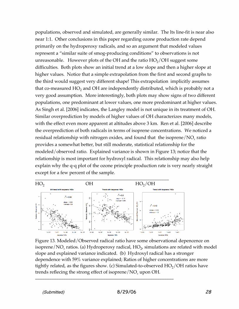
populations, observed and simulated, are generally similar. The lts line-fit is near also near 1:1. Other conclusions in this paper regarding ozone production rate depend primarily on the hydroperoxy radicals, and so an argument that modeled values represent a “similar suite of smog-producing conditions” to observations is not unreasonable. However plots of the OH and the ratio HO2/OH suggest some difficulties. Both plots show an initial trend at a low slope and then a higher slope at higher values. Notice that a simple extrapolation from the first and second graphs to the third would suggest very different shape! This extrapolation implicitly assumes that co-measured HO2 and OH are independently distributed, which is probably not a very good assumption. More interestingly, both plots may show signs of two different populations, one predominant at lower values, one more predominant at higher values. As Singh et al. [2006] indicates, the Langley model is not unique in its treatment of OH. Similar overprediction by models of higher values of OH characterizes many models, with the effect even more apparent at altitudes above 3 km. Ren et al. [2006] describe the overprediction of both radicals in terms of isoprene concentrations. We noticed a residual relationship with nitrogen oxides, and found that the isoprene/NOx ratio provides a somewhat better, but still moderate, statistical relationship for the modeled/observed ratio. Explained variance is shown in Figure 13; notice that the relationship is most important for hydroxyl radical. This relationship may also help explain why the q-q plot of the ozone principle production rate is very nearly straight except for a few percent of the sample. _________________________________________________________ HO2 OH HO2/OH

Figure 13. Modeled/Observed radical ratio have some observational depencence on isoprene/NOx ratios. (a) Hydroperoxy radical, HO2, simulations are related with model slope and explained variance indicated. (b) Hydroxyl radical has a stronger dependence with 59% variance explained; Ratios of higher concentrations are more tightly related, as the figures show. (c) Simulated-to-observed HO2/OH ratios have trends reflecing the strong effect of isoprene/NOx upon OH. ___________________________________________________________


Do other simple statistical relationships describe these radicals? Rohrer and Berresheim [2005] recently reported a sampling site at which OH was strongly related to just one variable important for its formation, the photolysis rate of ozone to O(1D), explaining ~90% of the variance of OH. In the airborne survey of many airmass situations over our continental region, we found only ~49% of the variance was explained. We have found that by considering the production and loss of peroxy radicals and the activity of CO in destroying OH as well, the statistical relationships explaining 72% or more of the variance can be estimated from easily made aircraft measurements [Chatfield et al., 2006]. Relations between simulated and observed radicals deserve more study, and these should be examined for implications regarding the predominant and total ozone production rates, despite the evidence of Figure B11 in the previous section. 3. Summary and Conclusions Ozone and contributors to its production over Central and Eastern North America were broadly sampled during July and August, 2004, a summer period of only moderate smog. The boundary layer and the region above it up to 3 km had relatively similar distributions of ozone concentration, and likely interacted over a few days time-scale. Ozone concentrations had a spatial autocorrelation structure reflecting interesting correlations at relatively local (100 km) and regional (800 km) scales. Extreme and rapidly variable variation of production of ozone characterized this region; common production rates were 1–3 ppb hr–1 and most ozone production during this period occurred at ozone levels of 40–50 ppb. Precursors like formaldehyde and NOx varied at shorter scales, dropping to 0.71 correlation at 25–30 km. Ozone formation rate processes were characterized by both a point model and by “principal terms.” The “principal production rate of ozone,” due to the reaction of HO2+NO, accounted for ~60% of total ozone production, according to the point model. The average spatial autocorrelation of principal production rate dropped to 0.71 autocorrelation at ~10 km or so, but there was autocorrelation out to the length-scale distance of ~60km. Temporal variability of ozone over one airport, Atlanta, was described by the MOZAIC aircraft sampling. Layers up to 2.5 km showed similar ozone concentrations and variability as ozone in the 0–1 km nominal boundary layer height. A strikingly simple but non-linear relationship was noted between a single “index variable,” jHCHO->rads x HCHO x NO, and the principal ozone production rate. A regression spline showed expected behavior, with ozone production rate increasing, but ever more slowly, as values of the index variable increased. This was attributed to


the non-linearity of ozone production and radical-radical reaction within the smog system. The fit described 89–91% of the variance of the principal ozone production term; this seems to indicate something of the inherent precision of the HO2, HCHO, and photolysis instruments. Point model simulations suggested that total ozone production was ~1.57 x the principal rate. Although there was considerable scatter in individual simulations, overall the model predicted similar ozone production rates. Still, the point model has several consistent deviations from the observations. Regression models confirmed that the model-to-observed ratios of OH and HO2 were consistently dependent on the isoprene-to-NOx ratio. For OH, about 60% of the variance of the modeled-to-simulated concentrations was explained by this ratio. Curiously, the probability distributions of simulated and observed rates of the significant reaction of HO2+NO are nearly 1:1. We are eager to test out these observations with even more widely varied conditions of lower tropospheric chemistry and hope that this first report can stimulate discussion and further testing. Acknowledgements: This work was supported by the NASA Tropospheric Chemistry Program. Considerable acknowledgement is given to the American Chemistry Council, who sponsored introductory research into the importance of aldehydes and nitrogen oxides downwind of North America, ATM-0008. Research into the spatial scales of ozone and precursors was inspired by NASA’s Aura Validation Program. Ronald Cohen, Timothy Bertram, and Anne Perring of U.C. Berkeley contributed nitrogen dioxide information. Thanks to Francis Binkowski of U. North Carolina for discussions.


Al-Saadi, J., R. B. Pierce, C. Kittaka, D. Fairlie, T. K. Schaack, D. R. Johnson,

T. H. Zapotocny, M. Avery, A. Thompson, R. Cohen, J. Dibb, J. Crawford, D. Rault, J. Szykman, R. Martin, Lagrangian Characterization of the Sources and Chemical Transformation of Air Influencing the Continental US During the 2004 ICARTT/INTEX-A Campaign

Bertram, T.H., A. Perring, P. Wooldridge, R. Cohen, J. Dibb, E. Scheuer, J. Crounse, P. Wennberg, S. Vay, S. Kim, G. Huey, J. Walega, A. Fried, M. Porter, H. Fuelberg, B. Heikes, G. Sachse, M. Avery and A. Clarke, Convection and the Age of Air in the Upper Troposphere, submitted to Science, 2006.

Blanchard, C. L., Lurman, F. W., Korc, M., and Roth, R. M.: The use of ambient data to corroborate analyses of ozone control strategies, Tech. Rep. STI-94030-1433-FR, Sonoma Technology Inc., 1994.

Browell, E. V., M. A. Fenn, J. W. Hair, C. F. Butler, A. Notari, S. A. Kooi, S. Ismail, M. A. Avery, R. B. Pierce, and H. E. Fuelberg, Large-scale Air Mass Characteristics Observed During the Summer Over North America and Western Atlantic Ocean, submitted to J. Geophys. Res., this issue, 2006.

Cantrell, C. A., R. E. Shetter, T. M. Gilpin, J. G. Calvert, F. L. Eisele and D. J. Tanner, J. Geophys. Res., 101, 14653, 1996.

Carmichael, G., Y. Tang, M. Mena + many, Regional-scale chemical transport modeling in support of the analysis of observations obtained during the ICARTT experiment, submitted to J. Geophys. Res., this issue, 2006.

Chameides, W. L., et al., Ozone precursor relationships in the ambient atmosphere, J. Geophys. Res., 97, 6037-6055, 1992.

Chatfield, R. B., et al., Evaluating the Empirical HCHO/NO Contour Plot Method for Smog Ozone and the POGO-FAN Technique, manuscript in preparation, 2006.

Davis, K.J., Surface fluxes of trace gases derived from convecitve layer profiles, Ph.D. dissertation, 281 pp., Univ. of Colo., Boulder, 1992 (Available as NCAR/CT-139 from NCAR, Boulder, Colo.)


Kleinman, L. I., Ozone procuess insights from field experiments – part II; observation-based analysis for ozone production. Atmos. Environ., 34, 2023-2034, 2000.

Lin, X., M. Trainer, and S. C. Liu, On the nonlinearity of tropospheric ozone production, J. Geophys. Res., 93, 15,879-15,888, 1988. Liu, S. C., M. Trainer, F. C. Fehsenfeld, D. D. Parrish, E. J. Williams, D. W. Fahey, G. Hubler, and P. C. Murphy, Ozone production in the rural troposphere and the implications for regional and global ozone distribution, J. Geophys. Res., 92, 4191-4207, 1987.

Lu, C-H. and J. S. Chang. On the indicator-based approach to assess ozone sensitivities and emissions features. J.Geophys. Res., 103, 3453-3462, 1998.

McKeen, S. A., E. -Y. Hsie, M. Trainer, R. Tallamraju, and S. C. Liu, A regional model study of the ozone budget in the eastern United States, J. Geophys. Res., 96, 10,809-10,845, 1991.

McKeen, S. A., G. Wotawa, D. D. Parrish, J. S. Holloway, M. P. Buhr, G. Hübler, F. C. Fehsenfeld, and J. F. Meagher Ozone production from Canadian wildfires during June and July of 1995, J. Geophys. Res., 107, doi: 10.1029/2001JD000697, 2002.

Milford, J.B., Gao, D., Sillman, S., Blossey, P. and Russell, A.G. (1994), "Total Reactive Nitrogen (NOy) as an Indicator of the Sensitivity of Ozone to Reductions in Hydrocarbon and NOx Emissions," J. Geophys. Res., 99: 3533-3542.

Rohrer, F., and H. Berresheim, Strong correlation between levels of tropospheric hydroxyl radicals and solar ultraviolet radiation Nature ,442, 184–187, 2006.

Shetter, R. E., and M. Muller (1999), Photolysis frequency measurements using actinic flux spectroradiometry during the PEM-Tropics mission: Instrumentation description and some results, J. Geophys. Res., 104, 5647–5661.

Fried, A., J. Walega, J. Olson, J. Crawford, G. Chen, B. Heikes, D. O' Sullivan, H. Shen, and many others where we use their data, The Role of Convection in Redistributing Formaldehyde to the Upper Troposphere over North America and the North Atlantic during the Summer 2004 INTEX Campaign.


Pfister, G. et al., Ozone Production from Boreal Forest Fire Emissions, 2006JD007695, this issue.

Ren, Xinrong, et al., HOx Observation and Model Comparison during INTEX-NA 2006JD007726, 2004.

Seinfeld, J.H, and Pandis, S.N., Atmospheric Chemistry and Physics from Air Pollution to Climate Change, John Wiley and Sons, 1998.

Sillman, S., The use of NOy, H2O2 and HNO3 as indicators for O3-NOx-VOC sensitivity in urban locations, J. Geophys. Res., 100, 14,175–14,188, 1995.

Sillman, S., and D. He, Some theoretical results concerning O3-NOx-VOC chemistry and NOx-VOC indicators, J. Geophys. Res., 107, 10.1029/2001JD001123, 2002.

Singh, H. B., W. Brune, J. Crawford, and D. Jacob, Overview of the Summer 2004 Intercontinental Chemical Transport Experiment-North America (INTEX-A).

Singh, H., Y. Chen, A. Staudt, D. Jacob, D. Blake, B. Heikes, and J. Snow, Evidence from the Pacific troposphere for large global abundances and sources of oxygenated organic compounds, Nature, 410, 1078-1081, 2001.

Trainer, M.,et al. . Correlation of ozone with NOy in photochemically aged air. J. Geophys. Res., 98, 2917-2926, 1993.

Thouret V., Cho J., Newell R., Marenco A. and Smit H., General characteristics of tropospheric trace constituent layers observed in the MOZAIC program, J. Geophys. Res., 105, 17,379-17,392, 2000.

Venables, W.N., and B.D. Ripley, Modern Applied Statistics with S. Fourth Edition, New York: Springer Verlag, 2002.

Documents

Smog Ozone Production over Eastern North America: HOx and