Smart Settlement

Mariana Khapko and Marius Zoican∗

May 1, 2018

Abstract

Recent regulatory and FinTech initiatives aim to streamline post-trade infrastructures.

Does faster settlement benefit markets? We build a model of intermediated trading with

flexible settlement and imperfectly competitive securities lending. Faster settlement

reduces counterparty risk, but increases borrowing needs. Rigid failure-to-deliver

penalties trigger a toxic rat race, as traders aim to lock in low borrowing costs. Excess

demand for fast settlement augments lenders’ rents. Optimal penalties resemble put

options on the security lending market: They protect traders against high settlement

costs, but do not eliminate failures-to-deliver. Flexible penalties discipline security

lender competition and facilitate faster trade settlement.

Keywords: Market design, trade settlement, security lending, counterparty risk

JEL Codes: D43, D47, G10, G20

∗Mariana Khapko is affiliated with University of Toronto and Rotman School of Management. Mar-ius Zoican is affiliated with Universite Paris-Dauphine. Mariana Khapko can be contacted at mari-ana.khapko@rotman.utoronto.ca. Marius Zoican can be contacted at marius-andrei.zoican@dauphine.fr.We have greatly benefited from discussion on this research with Matthieu Bouvard, Sabrina Buti, Jean-Edouard Colliard, Gilles Chemla, Olivier Dessaint, Bjorn Hagstromer, Carole Gresse, Sean Foley, ThierryFoucault, Florian Heider, Andrei Kirilenko, Charles-Albert Lehalle, Katya Malinova, Albert Menkveld, SophieMoinas, John Nash, Maureen O’Hara, James Thompson, Tomas Thornqvist, Emiliano Pagnotta, AndreasPark, Christine Parlour, Batchimeg Sambalaibat, Liyan Yang, Darya Yuferova, and Haoxiang Zhu. We aregrateful to conference participants at the 2017 NBER Meeting on Competition and the Industrial Organizationof Securities Markets, the 2017 SFS Cavalcade, 2017 EFA Meeting, the 13th Central Bank Conference on theMicrostructure of Financial Markets, the Swedish House of Finance FinTech Conference, 2017 NFA Meeting,2017 SFA Meeting, 2nd FIRN Market Microstructure Meeting, Eighth Erasmus Liquidity Conference, TwelfthEarly Career Women in Finance Conference, 10th Risk Management Forum in Paris, 2nd Financial MarketInfrastructure Conference, IRMC 2017, IFABS 2017, FEBS 2017, Toronto FinTech Conference 2017, as wellas to seminar participants at University of Toronto, HKUST, Toulouse School of Economics, HEC Paris, KULeuven, Norwegian School of Economics, Tilburg University, WHU Vallendar, SAFE Frankfurt, Authoritede Marches Financiers, Stockholm Business School, ESCP Europe, Luxembourg School of Finance, andUniversite Paris-Dauphine for insightful comments. Mariana Khapko gratefully acknowledges Universityof Toronto and the Connaught Fund for a research grant. Marius Zoican gratefully acknowledges InstituteEuroplace de Finance for a research grant.

Smart Settlement

Abstract

Recent regulatory and FinTech initiatives aim to streamline post-trade infrastructures.

Does faster settlement benefit markets? We build a model of intermediated trading with

flexible settlement and imperfectly competitive securities lending. Faster settlement

reduces counterparty risk, but increases borrowing needs. Rigid failure-to-deliver

penalties trigger a toxic rat race, as traders aim to lock in low borrowing costs. Excess

demand for fast settlement augments lenders’ rents. Optimal penalties resemble put

options on the security lending market: They protect traders against high settlement

costs, but do not eliminate failures-to-deliver. Flexible penalties discipline security

lender competition and facilitate faster trade settlement.

Keywords: Market design, trade settlement, security lending, counterparty risk

JEL Codes: D43, D47, G10, G20

1 Introduction

How fast should trades be settled? A number of recent reforms showcase markets’ appetite

for faster settlement: In September 2017, the U.S. and Canadian markets migrated from a

three-day (T+3) to a two-day (T+2) settlement cycle for equity transactions. Previously,

European equity markets had transitioned to T+2 in 2014; Singapore and Japan plan similar

reforms in 2018 and 2019, respectively.

Faster settlement reduces counterparty risk. A Boston Consulting Group study (BCG,

2012) commissioned by the Depository Trust & Clearing Corporation (DTCC) estimated a

38% (USD 1 bln) market-wide drop in counterparty risk exposure following U.S. markets’

transition from T+3 to T+2. Indeed, a significant number of trades, both exchange-based

and OTC, fail to settle on time every day. Reuters estimates that, on an average trading day

in 2011, failures-to-deliver on the U.S. equity market reached 4.3% of total traded volume. In

1995, under a five-day settlement cycle, the U.S. equity failure-to-deliver rate amounted to

8.43% (Levitt, 1996). The failure rate is even higher and more volatile for other asset classes:

In the week of March 9, 2016, trade failures in U.S. government bonds spiked at $456bn

compared to a weekly average of $94bn the year before.1

Faster settlement, however, is costly. First, the migration process itself requires a complete

overhaul of back-office processes. Second, and more importantly, faster settlement requires

broker-dealers to either borrow the securities they need to settle, or to pre-position their

trades, and therefore to carry inventory risk. Security lenders typically wield market power, as

demonstrated, for example, by recent U.S. lawsuits in 2017 filed by pension funds. Anecdotal

evidence suggests that these costs are important: In 2013, the Moscow Stock Exchange

transitioned from immediate settlement to T+2, citing security borrowing costs as a key

rationale.2

Our paper formalizes the trade-off between counterparty risk and security borrowing

costs. On the one hand, a long delay between trade and settlement increases exposure to

counterparty risk. On the other hand, a short settlement cycle augments expected security

borrowing costs. The paper’s contribution is (i) to study the impact of settlement cycle

length and flexibility on market quality, as well as (ii) to establish the optimal structure of

failure-to-deliver penalties.

1The sources for this paragraph are the Reuters’ 2012 article Persistent trade failure problem gets partialfix, and Financial Times’ 2016 article Trade failures of US bonds hit $456bn.

2See Reuters, U.S. pension funds sue Goldman, JPMorgan, others over stock lending market (2017); alsoBloomberg’s 2013 article Moscow Targets March Move to 2 Day Settlement.

1

Regulators have long envisioned the possibility of flexible trade settlement. In 1996,

following the U.S. markets’ migration from a five- to a three-day settlement cycle, the Securi-

ties and Exchange Commission (SEC) chairman Arthur Levitt emphasized the “staggering

interdependence” between financial infrastructures in trade settlement and called for a less

rigid system to accommodate the preferences of individual investors (Levitt, 1996). Currently,

each trade needs to be processed by a number of different institutions from execution on

the exchange until settlement, such as brokerage firms, custodian banks, clearing agencies,

and central securities depositories. In a landscape in which traders can update quotes with

nanosecond frequency, the state of post-trade financial infrastructure feels dated.

New technologies such as distributed ledgers (e.g., but not limited to, Blockchain) could

facilitate the implementation of flexible settlement chains. For instance, in April 2018,

the Australian Stock Exchange (ASX) revealed a detailed plan to implement distributed

ledger technology (DLT) for securities settlement before 2021. The new system would offer

traders the option to settle their trades earlier than T+2.3 Furthermore, failure-to-deliver

contingencies could be accounted for by the use of “smart contracts” (defined by Cong and

He, 2018 as self-enforcing digital contracts with automated execution). For example, ASX

plans to introduce mandatory automatic security borrowing to rule out failures-to-deliver.

We build a model of interconnected security trading and security lending (repo) markets,

with delivery-versus-payment settlement, in which we introduce three frictions.4 First,

buyers and sellers arrive asynchronously at the market (as in Grossman and Miller, 1988)

and therefore trading is intermediated. Second, intermediaries can exogenously default:

consequently, traders bear counterparty risk. Third, the lending supply is limited and the

security lending market is opaque. As in Duffie, Garleanu, and Pedersen (2002), security

lenders can earn rents and borrowing is costly for intermediaries. We distinguish between

default and failure-to-deliver: Trades which fail to deliver are eventually settled if the

intermediary does not default before locating the asset.

Our main result is that traders’ utility is maximized by a contract featuring immediate

settlement and a flexible failure-to-deliver penalty. The flexible penalty implements an

incentive compatible contract between buyers and intermediaries. That is, an intermediary

3See ASX, CHESS Replacement: New Scope and Implementation Plan, April 2018. Other exchangesexpress a similar interest in DLT and trade settlement flexibility: Fredrik Voss, VP of Blockchain Innovationat Nasdaq, acknowledges DLT would “allow participants to select the pace at which they want to settle, whichhas been challenging to do in the market today.” (https://goo.gl/mv68il).

4Tobias, Begalle, Copeland, and Martin (2013) point out that securities lending and repo agreements areeconomically similar, albeit used in the context of different asset classes. In this paper, we use the two termsinterchangeably.

2

only accesses the repo market when the cost of borrowing securities is lower than the marginal

counterparty risk it imposes on a buyer through a failure-to-deliver. The optimal penalty is

equivalent to a put option written on the repo market price, where the “strike price” increases

in counterparty risk and trading urgency. Importantly, the optimal contract does not rule

out failures-to-deliver in equilibrium.

An exogenous, large failure-to-deliver penalty ensures that all trades are settled on time,

as intermediaries always borrows securities if needed.5 In this case, immediate settlement is

not necessarily optimal. If borrowing costs are large, counterparty risk is low, or both, buyers

prefer delayed settlement instead. A longer time-to-settlement allows intermediaries more

time to wait for an opposite-side trade, which reduces the likelihood to borrow securities.

Intuitively, the optimal settlement time decreases in intermediaries’ default risk. If repo

markets are perfectly competitive, settlement flexibility allows traders with higher urgency to

reduce counterparty risk by settling before others, at a higher price.

If repo markets are not competitive, and if the regulator rules out failures-to-deliver by

imposing a large penalty, flexibility leads to a toxic settlement rat race. The intuition is that

a larger lending supply strengthens competition between security lenders, and lowers repo

borrowing costs for intermediaries. Trades which settle first consume part of the available

lending supply, consequently increasing borrowing costs for all future trades to be settled. It

follows that each buyer has an incentive to settle before everyone else. Two equilibria can

obtain, depending on model parameters: an immediate settlement equilibrium and a delayed

settlement equilibrium, where buyers randomize between a continuum of positive settlement

delays and, potentially, also immediate settlement. The settlement rat race is costly as it

leads to shorter-than-optimal settlement cycles, excessive security borrowing activity, and

economic rents for security lenders.

A flexible failure-to-deliver penalty eliminates the settlement rat race as it stimulates

competition between security lenders. In equilibrium, the penalty increases in counterparty

risk. For low counterparty risk, intermediaries are given weaker incentives to borrow. There-

fore, security lenders compete stronger on prices in order to attract intermediaries. For

high counterparty risk, security lenders’ rents are larger as they are better able to hold

up intermediaries who face higher failure penalties. In equilibrium, trades fail to deliver

if counterparty risk is low. Further, the failure-to-deliver rate increases in the security’s

specialness, that is the opportunity cost to supply an instrument on the security lending

5Currently, the Fixed Income Clearing Corporation (FICC) sets a failure-to-deliver penalty at 3% on thesettlement value of the trade (minus the Target Fed funds rate in effect the day before the settlement day).

3

market.

In sum, the paper’s message is that a flexible or a short settlement cycle (i.e, T+0),

coupled with an option-like penalty for failures-to-deliver, disciplines competition on securities

lending markets and therefore improves market quality. Our results support the ongoing

reforms around the globe to shorten settlement cycles, and offer insights on how to reduce

the costs associated with fast settlement.

2 Related Literature

Our paper contributes to an active discussion on the design of post-trade financial infrastruc-

tures. It relates to several branches of literature in the field of market microstructure and

financial innovation.

Literature on the securities lending market. D’Avolio (2002) provides a comprehensive

overview of the U.S. securities lending market. Large custodian banks are among the most

important lenders, acting on behalf of institutional traders such as pension or mutual funds,

and especially passive indexeres (i.e., ETFs). Security borrowers are either (i) specialists and

market-makers matching buy and sell orders, (ii) derivative traders hedging their positions,

or (iii) speculators taking outright short positions. IHS Markit (2016) estimates the global

supply of securities in lending programs at USD 15 trillion, generating USD 8.06 billion in

lending revenues for the year 2016.

Security lending markets typically exhibit imperfect competition. Chague, De-Losso,

Genaro, and Giovannetti (2017) study the Brazilian equity lending market and find that

borrowers with higher search costs face higher loan fees. In the same spirit, Huszar and

Simon (2018) document that German treasuries lenders behave as oligopolists. Perhaps the

most closely related paper to ours, Duffie, Garleanu, and Pedersen (2002) model the security

lending market as a sequential Nash bargaining game, where high search costs allow security

lenders to extract economic rents from borrowers. Trade prices are determined on a Walrasian

spot market. In contrast, buyers and sellers in our model arrive at the market asynchronously

(as in, e.g., Grossman and Miller, 1988), and trading is intermediated. Therefore, a longer

settlement delay improves the likelihood of a match on the spot market, and reduces expected

security borrowing costs. We solve for the optimal incentive compatible intermediation

contract and the corresponding failure-to-deliver penalty.

4

Beyond imperfect competition, lending fees also depend on the opportunity or transaction

costs to supply an instrument on the security lending market. Small-cap, non-index, or illiquid

stocks are more difficult to borrow, as are stocks with concentrated ownership (for example,

around initial public offerings, as in Geczy, Musto, and Reed, 2002). Duffie (1996) refers

to such lending constraints as part of a security’s specialness and argues that specialness

drives up prices. Indeed, Jordan and Jordan (1997) document a liquidity premium for repo

specialness for on-the-run U.S. Treasuries. Further, D’Avolio (2002) finds that lending fees

can reach “spectacular heights,” that is more than 55% in annualized terms.

Several empirical papers show that the supply of securities available for lending correlates

with liquidity and failures-to-deliver. Foley-Fisher, Gissler, and Verani (2017) find that the

collapse of AIG’s security lending programs in 2008 caused a substantial and long-lasting

reduction in market liquidity for corporate bonds. Corradin and Maddaloni (2017) document

that the 2011 outright purchase program of the Eurosystem for Italian sovereign bonds, which

reduced their supply, increased borrowing costs and led to more fail-to-deliver transactions.

Finally, Huszar and Simon (2018) find that the withdrawal of German banks from security

lending markets around year’s end, for financial reporting purposes, reduces the supply of

lendable securities and increases lending fees. In our model, failures-to-deliver occur with

positive probability even if the optimal contract is implemented, and are more likely if the

security is in limited supply.

Literature on counterparty risk. We also contribute to a strand of literature studying

counterparty risk. In the aftermath of the 2007-2009 financial crisis, several papers focus

the impact of a central clearing counterparty on market quality (Acharya and Bisin, 2014,

Acharya, 2009, Pirrong, 2009, Stephens and Thompson, 2017). Loon and Zhong (2014)

document that counterparty risk is priced by the market and that the introduction of a CCP

in 2009, following the Dodd-Frank Act, led to a decrease in counterparty risk in the CDS

market. Duffie and Zhu (2011) discuss economies of scope from having a single CCP across

all asset classes. To control systemic risk, Menkveld (2017) proposes a collateral system that

internalizes the global effects of highly correlated portfolios across traders, i.e., the “crowding

risk.” Failures-to-deliver may be caused by miscommunication and operational problems, a

failure to receive the assets from an unrelated trade, or short selling (Fleming and Garbade,

2005). Evans, Moussawi, Pagano, and Sedunov (2017) and Fotak, Raman, and Yadav (2014)

focus on failures-to-deliver driven by short-selling and find a negative correlation between

liquidity and settlement risk.

5

Central counterparties’ main benefit comes through netting existing positions, that is

reducing the size of risk exposure. Our paper complements the existing counterparty risk

literature by focusing on the length of risk exposure.

Literature on financial infrastructure technology. Finally, our paper contributes to

a small, yet rapidly growing literature on financial technology in securities markets. We argue

that flexible settlement and fail-to-deliver penalties, as implemented for example by smart

contracts on a distributed ledger, improve market quality. Malinova and Park (2017) refer to

distributed ledgers and smart contracts as “the technology that enables frictionless transfer

of value.” The regulatory consensus is that distributed ledger technology can eliminate the

need for multiple records of a single trade and consequently reduce the number of post-trade

intermediaries (ECB, 2016, ESMA, 2016, Brainard, 2016). Investments are already underway:

In January 2017, the Depository Trust and Clearing Corporation (DTCC), which processes

$1.5 quadrillion in trades a year, announced a plan to deploy DLT technology for post-trade

processing in early 2018.6

Benos, Garratt, and Gurrola-Perez (2017) argue that distributed ledgers have the potential

to improve efficiency and reduce costs in securities settlement. Koeppl and Chiu (2018) find

that large trading volume and strong preferences for fast settlement are necessary conditions

for the viability of a public, anonymous Blockchain trade settlement system.7 We argue

that immediate settlement can indeed be optimal, provided there is enough flexibility in

failure-to-deliver penalties.

3 Model

3.1 Model primitives

Asset. Consider a continuous-time economy. As in Kyle and Obizhaeva (2017), the game

ends at an arbitrarily large but finite T , at which time utilities are evaluated. A single asset

pays off a stochastic dividend v ∼ N (0, σ2) at T . The discount rate is normalized to zero.

6See Forbes report from January 9, 2017.7A number of papers are also studying the feasibility of trading on a public blockchain: Biais, Bisiere,

Bouvard, and Casamatta (2018), Aune, O’Hara, and Slama (2017), and Saleh (2017).

6

Agents. There are four types of agents in the economy: two identical buyers, two competitive

intermediaries, one large seller, and a large number of risk-averse security lenders.8 Security

lenders are typically institutional investors such as pension funds, who we think of as more

risk-averse than high-frequency traders or market-makers. Buyers, intermediaries, and sellers

are risk-neutral.

Buyers (B) can only trade at t = 0 and have no endowment of the risky asset. Buyers

trade to lock in a private value θ > 0 for the first unit of the risky asset.

Intermediaries (I), unlike buyers, are always present at the market. They have no

endowment of the risky asset and no private values. Further, intermediaries have access to a

risk-free productive technology yielding R > 1 at T for every unit invested at t = 0, standing

in for the intermediaries’ shadow cost of capital. They can partially liquidate the investment

at any point in time, but cannot reinvest. Intermediaries may exogenously default (e.g., due

to shocks in unrelated business activities). The default time is exponentially distributed with

rate parameter δ, that is, the probability of default before t is

P (Default < t) = 1− exp (−δt) . (1)

The large seller (S) has an endowment of at least two units of the risky asset. She arrives

at the market at a random time which follows an exponential distribution with rate parameter

λ. The large seller arrives at the market before t with probability

P (Seller < t) = 1− exp (−λt) . (2)

Security lenders (L) have mean-variance preferences. There are N lenders with risk-

aversion coefficient γ and a competitive fringe of lenders with risk-aversion Γ > γ.9 With

probability ϕ, each lender owns a unit of the risky asset as a perfect hedge for an endowment

of an asset that pays off −v. Ownership of the risky asset is private information for each

lender. A lower ϕ corresponds to higher specialness of the security.

Two assumptions about security lenders are particularly important. First, security lenders

have heterogenous costs of supplying the asset. Second, the lendable supply is limited in

the following sense: The competitive supply schedule is not perfectly elastic, and therefore

8The model could be extended to feature an arbitrary number of buyers and intermediaries withoutaltering the economic trade-offs. The present setup is chosen to ease exposition. In particular, the buyersneed not be matched with different intermediaries.

9Normalizing γ = 0, that is assuming some security lenders are risk-neutral, does not change the modelresults. A positive γ > 0 allows for an equilibrium contract in which the intermediary never borrows the asset.

7

intermediaries cannot borrow large quantities without moving the repo price. We choose to

model the lending cost heterogeneity through variation in risk aversion. Alternatively, one

can model such heterogeneity as variation in search costs. For example, not all prime brokers

have access to electronic security lending platforms such as EquiLend. Further, opacity is a

realistic feature of security lending markets. In the model, the opacity assumption allows us

to back out a non-trivial cross-sectional distribution of repo haircuts. However, the results

largely go through also if we assume a transparent repo market.

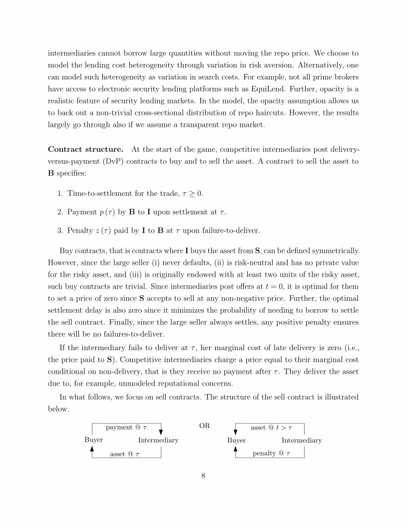
Contract structure. At the start of the game, competitive intermediaries post delivery-

versus-payment (DvP) contracts to buy and to sell the asset. A contract to sell the asset to

B specifies:

1. Time-to-settlement for the trade, τ ≥ 0.

2. Payment p (τ) by B to I upon settlement at τ .

3. Penalty z (τ) paid by I to B at τ upon failure-to-deliver.

Buy contracts, that is contracts where I buys the asset from S, can be defined symmetrically.

However, since the large seller (i) never defaults, (ii) is risk-neutral and has no private value

for the risky asset, and (iii) is originally endowed with at least two units of the risky asset,

such buy contracts are trivial. Since intermediaries post offers at t = 0, it is optimal for them

to set a price of zero since S accepts to sell at any non-negative price. Further, the optimal

settlement delay is also zero since it minimizes the probability of needing to borrow to settle

the sell contract. Finally, since the large seller always settles, any positive penalty ensures

there will be no failures-to-deliver.

If the intermediary fails to deliver at τ , her marginal cost of late delivery is zero (i.e.,

the price paid to S). Competitive intermediaries charge a price equal to their marginal cost

conditional on non-delivery, that is they receive no payment after τ . They deliver the asset

due to, for example, unmodeled reputational concerns.

In what follows, we focus on sell contracts. The structure of the sell contract is illustrated

below.

IntermediaryBuyer

payment @ τ

asset @ τ

IntermediaryBuyer

penalty @ τ

asset @ t > τOR

8

Timing. At t = 0, buyers arrive at the market and either choose one of the contracts posted

by the intermediaries, or do not trade. When the large seller arrives, she enters a contract

with one or more intermediaries: The large seller’s contracts settle immediately with a price

of zero.

I posts contracts

t = 0

B enters a trade

I receives the assetfrom S

I does not receivethe asset from S

I delivers the asset to B

t = τ

B pays p (τ) to I

I enters repo with LI delivers the asset to BB pays p (τ) to I

I fails to deliver to BI pays z (τ) to B

t > τ

I returns the asset to L

I delivers the asset to B

At τ , the intermediary needs to deliver the asset to the buyer. If she does not hold

the asset, the intermediary can enter a repurchasing contract with a security lender, to be

detailed below.10 Otherwise, the intermediary fails to settle: I pays z (τ) to the buyer at τ

and delivers the asset upon arrival of the seller at t > τ . At t = T , payoffs are realized.

Repurchase agreements. The intermediary can enter a repurchasing agreement (repo)

with a security lender at τ . In the start leg of the contract, the intermediary I pays ` to the

security lender L in exchange for the risky asset. To pay `, the intermediary liquidates part

of the risk-free investment, at cost R`. In the close leg of the contract, I delivers the risky

asset to L and L repays `′ to I. The repo contract is fully collateralized in the following sense:

The lender is perfectly hedged against the risk of the intermediary defaulting on the repo

contract (i.e., not returning the risky asset). Finally, the repo market is opaque: each lender

posts two prices ` and `′ and is unaware of other lenders’ offers.

Let b be the (potentially random) minimum borrowing cost for the intermediary across

all security lenders who own the asset, that is

b = mini∈L

R`i − `′i. (3)

10For tractability, we assume the intermediary borrows the security at the settlement time τ . Alternatively,the intermediary can be allowed to choose the optimal borrowing time before τ . Rational expectationscompetitive equilibria under the two specifications are isomorphic since buyers perfectly anticipate andincorporate the intermediaries’ strategies.

9

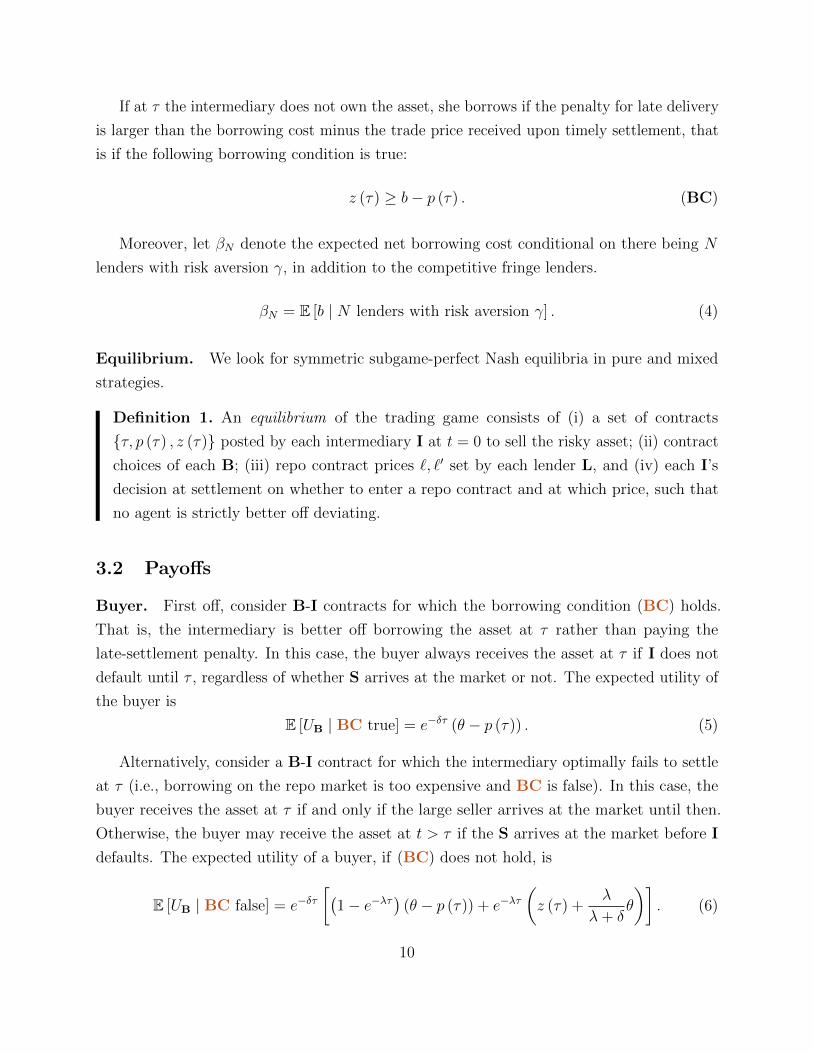
If at τ the intermediary does not own the asset, she borrows if the penalty for late delivery

is larger than the borrowing cost minus the trade price received upon timely settlement, that

is if the following borrowing condition is true:

z (τ) ≥ b− p (τ) . (BC)

Moreover, let βN denote the expected net borrowing cost conditional on there being N

lenders with risk aversion γ, in addition to the competitive fringe lenders.

βN = E [b | N lenders with risk aversion γ] . (4)

Equilibrium. We look for symmetric subgame-perfect Nash equilibria in pure and mixed

strategies.

Definition 1. An equilibrium of the trading game consists of (i) a set of contracts

τ, p (τ) , z (τ) posted by each intermediary I at t = 0 to sell the risky asset; (ii) contract

choices of each B; (iii) repo contract prices `, `′ set by each lender L, and (iv) each I’s

decision at settlement on whether to enter a repo contract and at which price, such that

no agent is strictly better off deviating.

3.2 Payoffs

Buyer. First off, consider B-I contracts for which the borrowing condition (BC) holds.

That is, the intermediary is better off borrowing the asset at τ rather than paying the

late-settlement penalty. In this case, the buyer always receives the asset at τ if I does not

default until τ , regardless of whether S arrives at the market or not. The expected utility of

the buyer is

E [UB | BC true] = e−δτ (θ − p (τ)) . (5)

Alternatively, consider a B-I contract for which the intermediary optimally fails to settle

at τ (i.e., borrowing on the repo market is too expensive and BC is false). In this case, the

buyer receives the asset at τ if and only if the large seller arrives at the market until then.

Otherwise, the buyer may receive the asset at t > τ if the S arrives at the market before I

defaults. The expected utility of a buyer, if (BC) does not hold, is

E [UB | BC false] = e−δτ[(

1− e−λτ)

(θ − p (τ)) + e−λτ(z (τ) +

λ

λ+ δθ

)]. (6)

10

With probability e−δτ(1− e−λτ

), S arrives at the market before τ and I does not default:

settlement occurs at τ , the buyer receives the asset and pays p (τ). With probability e−(δ+λ)τ ,

I pays penalty z (τ) to the buyer at τ . In this case, the probability of late settlement, for a

large T , can be approximated by

limT→∞

∫ T

τ

∫ x

τ

λδe−λy−δx dy dx+

∫ ∞

T

δe−δx dx = e−(λ+δ)τ λ

λ+ δ. (7)

Intermediary. The expected utility of the intermediary can be written as

EUI = e−δTE [UI | I survives] , (8)

where exp (−δT ) is the probability that I does not default until the end of the game. The

expected utility of the intermediary, conditional on survival until T , is:

E [UI | I survives] =(1− e−λτ

)p (τ) + e−λτE [max p (τ)− b,−z (τ)] . (9)

With probability 1− exp (−λτ), S arrives at the market until τ . The intermediary buys the

asset from the large seller at a price of zero, delivers it at τ to B and cashes in the price p (τ).

With the complementary probability, S does not arrive until τ . The intermediary chooses the

best of two options: either to pay the penalty z (τ), or to enter a repo agreement with L at

net cost b and deliver at τ against the payment p (τ).

Competitive intermediaries earn no excess profits in equilibrium. Since T is an arbitrarily

large number, exp (−δT ) is a very small, but positive probability. From equation (8), it

follows that the competitive condition is equivalent to setting the conditional expected utility

in equation (9) to zero.

Lender. The lender L receives the repo price ` if the intermediary enters a repurchase

agreement at τ . If the intermediary does not return the asset, the security lender is exposed

to his initial endowment of −v and has expected utility:

E [UL | I does not return the asset] = `− g

2σ2 ≥ 0⇒ ` ≥ g

2σ2, for g ∈ γ,Γ . (10)

If the intermediary returns the asset, the lender is perfectly hedged against his initial

11

endowment and has expected utility

E [UL | I returns the asset] = `− `′. (11)

We restrict our attention to repurchasing agreements that provide a perfect hedge for the

lender against the intermediary not returning the asset, it must be that11

E [UL | I does not return the asset] = E [UL | I returns the asset]⇒ `′ =g

2σ2. (12)

4 Benchmark equilibrium

In this section, we illustrate how the settlement delay τ drives the key trade-off between

counterparty risk and transaction costs. As a point of reference, we consider a variant of the

model under two simplifying assumptions.

First, we set N = 0 so that intermediaries may only borrow the risky asset from the

competitive fringe of security lenders. In Section 5 we allow for N > 0, and consequently

introduce imperfect competition between security lenders on an opaque repo market. Second,

we assume the failure-to-deliver penalty z is set exogenously (e.g., by a regulator) and is large

enough such that (BC) is always true. This assumption is consistent with, for example, the

exchange-mandated automatic borrowing feature proposed by the Australian Stock Exchange.

We further assume a large enough private value, such that the buyer has positive expected

utility from immediate settlement. This is the case if θ > β0, where β0 is defined in (4). In

Section 6, the buyer and intermediary can contract on the penalty in the contract, allowing

for endogenous failures-to-deliver when (BC) is false.

Security lenders in the competitive fringe obtain zero expected utility. Therefore, from

equation (10), each lender in the competitive fringe offers a repo price ` = Γ2σ2. Consequently,

the borrowing cost for the intermediary is β0, where from equation (4) it follows that

β0 = R`︸︷︷︸open leg

− `′︸︷︷︸close leg

=Γ

2σ2 (R− 1) . (13)

Intuitively, the borrowing cost increases in the lender’s risk-aversion, asset volatility, and the

opportunity cost of the intermediary (i.e., the safe investment return).

11A natural requirement for the repo contract is that the lender is never worse off if the intermediaryreturns the asset, that is `′ ≤ g

2σ2 for g ∈ γ,Γ.

12

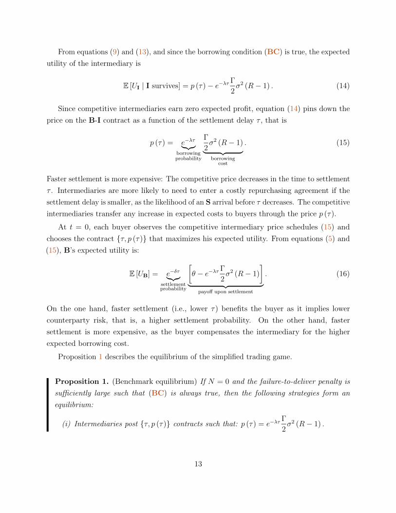
From equations (9) and (13), and since the borrowing condition (BC) is true, the expected

utility of the intermediary is

E [UI | I survives] = p (τ)− e−λτ Γ

2σ2 (R− 1) . (14)

Since competitive intermediaries earn zero expected profit, equation (14) pins down the

price on the B-I contract as a function of the settlement delay τ , that is

p (τ) = e−λτ︸︷︷︸borrowingprobability

Γ

2σ2 (R− 1)

︸ ︷︷ ︸borrowing

cost

. (15)

Faster settlement is more expensive: The competitive price decreases in the time to settlement

τ . Intermediaries are more likely to need to enter a costly repurchasing agreement if the

settlement delay is smaller, as the likelihood of an S arrival before τ decreases. The competitive

intermediaries transfer any increase in expected costs to buyers through the price p (τ).

At t = 0, each buyer observes the competitive intermediary price schedules (15) and

chooses the contract τ, p (τ) that maximizes his expected utility. From equations (5) and

(15), B’s expected utility is:

E [UB] = e−δτ︸︷︷︸settlementprobability

[θ − e−λτ Γ

2σ2 (R− 1)

]

︸ ︷︷ ︸payoff upon settlement

. (16)

On the one hand, faster settlement (i.e., lower τ) benefits the buyer as it implies lower

counterparty risk, that is, a higher settlement probability. On the other hand, faster

settlement is more expensive, as the buyer compensates the intermediary for the higher

expected borrowing cost.

Proposition 1 describes the equilibrium of the simplified trading game.

Proposition 1. (Benchmark equilibrium) If N = 0 and the failure-to-deliver penalty is

sufficiently large such that (BC) is always true, then the following strategies form an

equilibrium:

(i) Intermediaries post τ, p (τ) contracts such that: p (τ) = e−λτΓ

2σ2 (R− 1) .

13

(ii) Buyers choose the contract with time-to-settlement equal to τ ?, where

τ ? = max

0,

1

λlog

[(δ + λ)

θδ

Γ

2σ2 (R− 1)

]. (17)

(iii) Competitive fringe security lenders set repo purchasing price ` =Γ

2σ2.

(iv) Intermediaries borrow the asset at τ ? if the large seller did not arrive before τ ?.

From equation (17), immediate settlement is optimal for high enough default risk δ or for

low enough borrowing costs, that is if

δ

δ + λθ ≥ β0 =

Γ

2σ2 (R− 1) . (18)

Corollary 1 provides comparative statics results for the equilibrium time-to-settlement in

the simplified game.

Corollary 1. (Benchmark comparative statics) The optimal time-to-settlement τ ? weakly

(i) increases in the lender’s risk aversion (Γ), asset volatility (σ), and the intermediary’s

opportunity cost (R), and

(ii) decreases in counterparty risk (δ) and buyer private value (θ).

Finally, there exists a Λ0 > 0 such that τ ? increases in λ for λ ≤ Λ0 and τ ? decreases in λ

for λ > Λ0.

Buyers choose the time-to-settlement τ ? that optimally trades off counterparty risk against

the expected repo borrowing cost. A higher default rate for the intermediary leads to faster

settlement in equilibrium. Conversely, buyers choose a longer settlement delay if the borrowing

cost is larger (either due to asset volatility, L’s risk-aversion, or opportunity costs for the

intermediary). A longer settlement delay increases the large seller’s arrival probability and

lowers the likelihood of a costly repo agreement.

From Proposition 1, it immediately follows that the equilibrium price paid by buyers upon

settlement at τ ? is:

p (τ ?) = min

δ

δ + λθ,

Γ

2σ2 (R− 1)

. (19)

14

If immediate settlement is optimal, I always enters a repo agreement: Therefore, the price

is equal to the net borrowing cost. Otherwise, if delayed settlement is optimal, the price paid

by B at τ ? increases in I’s default rate and buyers’ private value as τ ? is lower and I is more

likely to borrow the risky asset. At the same time, the settlement price decreases in the large

seller’s arrival rate as borrowing is less likely for higher λ.

The large seller arrival rate λ has a non-linear impact on the equilibrium time-to-settlement.

In markets with plenty of potential sellers, that is for very high λ, buyers choose fast settlement

as it yields both low counterparty risk and a sufficiently low likelihood of I entering a repo

agreement (formally, limλ→∞ τ? = 0). On the other hand, in markets with very few potential

sellers, that is for low λ, there are no perfect options: The buyer can either choose immediate

settlement and agree to compensate the intermediary for the borrowing cost, or choose a long

settlement delay and accept the corresponding counterparty risk. If the borrowing cost is low,

the buyers’ private value is high, or both, then buyers choose fast settlement in both very

thick and very thin markets (high and low λ), and therefore the optimal time-to-settlement

first increases and then decreases in the seller’s arrival rate.

Figure 1 illustrates the optimal time-to-settlement and corresponding B-I settlement price

as functions of the intermediary’s default risk (δ) and the seller’s arrival rate (λ).

[ insert Figure 1 here ]

5 A settlement rat race

In this section, we allow for N ≥ 2 and therefore introduce imperfect competition between the

N security lenders with low risk-aversion γ < Γ. As in Section 3, we assume that (i) buyer’s

private value is large enough, that is θ > β0, and that (ii) (BC) is true and therefore the

intermediary always borrows at the settlement time if she does not have the asset. We show

that imperfect competition between security lenders, due to the opacity of the repo market,

generates a settlement rat race in which buyers choose sub-optimally short settlement delays.

5.1 Competition on the repo market

From equation (10), each of the N security lenders with risk-aversion γ requires a large

enough repo price, that is ` ≥ γ2σ2, in order to lend the asset to I. Since intermediaries

15

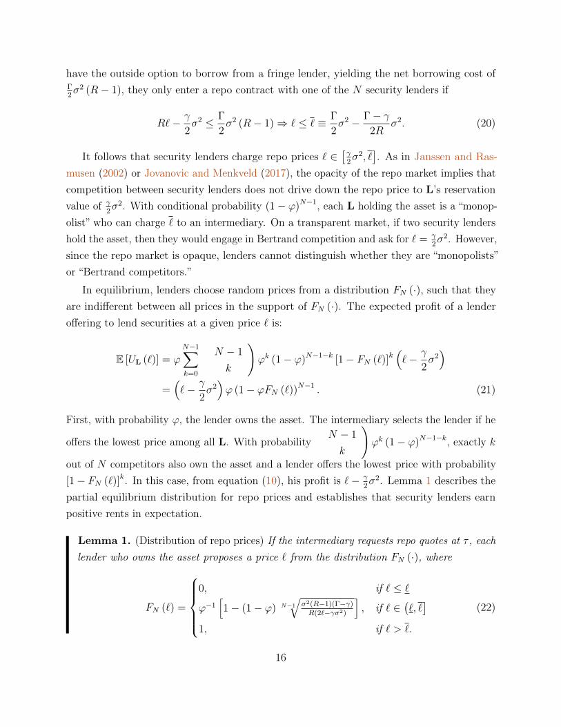
have the outside option to borrow from a fringe lender, yielding the net borrowing cost ofΓ2σ2 (R− 1), they only enter a repo contract with one of the N security lenders if

R`− γ

2σ2 ≤ Γ

2σ2 (R− 1)⇒ ` ≤ ` ≡ Γ

2σ2 − Γ− γ

2Rσ2. (20)

It follows that security lenders charge repo prices ` ∈[γ2σ2, `

]. As in Janssen and Ras-

musen (2002) or Jovanovic and Menkveld (2017), the opacity of the repo market implies that

competition between security lenders does not drive down the repo price to L’s reservation

value of γ2σ2. With conditional probability (1− ϕ)N−1, each L holding the asset is a “monop-

olist” who can charge ` to an intermediary. On a transparent market, if two security lenders

hold the asset, then they would engage in Bertrand competition and ask for ` = γ2σ2. However,

since the repo market is opaque, lenders cannot distinguish whether they are “monopolists”

or “Bertrand competitors.”

In equilibrium, lenders choose random prices from a distribution FN (·), such that they

are indifferent between all prices in the support of FN (·). The expected profit of a lender

offering to lend securities at a given price ` is:

E [UL (`)] = ϕN−1∑

k=0

(N − 1

k

)ϕk (1− ϕ)N−1−k [1− FN (`)]k

(`− γ

2σ2)

=(`− γ

2σ2)ϕ (1− ϕFN (`))N−1 . (21)

First, with probability ϕ, the lender owns the asset. The intermediary selects the lender if he

offers the lowest price among all L. With probability

(N − 1

k

)ϕk (1− ϕ)N−1−k, exactly k

out of N competitors also own the asset and a lender offers the lowest price with probability

[1− FN (`)]k. In this case, from equation (10), his profit is `− γ2σ2. Lemma 1 describes the

partial equilibrium distribution for repo prices and establishes that security lenders earn

positive rents in expectation.

Lemma 1. (Distribution of repo prices) If the intermediary requests repo quotes at τ , each

lender who owns the asset proposes a price ` from the distribution FN (·), where

FN (`) =

0, if ` ≤ `

ϕ−1[1− (1− ϕ) N−1

√σ2(R−1)(Γ−γ)R(2`−γσ2)

], if ` ∈

(`, `]

1, if ` > `.

(22)

16

and ` =σ2

2

[γ + (Γ− γ)

R− 1

R(1− ϕ)N−1

]. The upper bound of the price distribution, `,

is defined in equation (20). Further, each lender earns positive expected rents

E [UL] = ϕ (1− ϕ)N−1 σ2

2(Γ− γ)

R− 1

R> 0. (23)

Let ΩL denote the set of lenders who own the asset. The expected net borrowing cost for

an intermediary, βN , is:

βN =[1− (1− ϕ)N

] (E[mini`i | ΩL 6= ∅

]×R− γ

2σ2)

+ (1− ϕ)NΓ

2σ2 (R− 1) . (24)

With probability 1− (1− ϕ)N , at least one of the N security lenders owns the asset and the

intermediaries choose the lowest price offered. With probability (1− ϕ)N , no security lender

with risk-aversion γ owns the asset, and the intermediaries need to borrow from the fringe

lenders at net cost Γ2σ2 (R− 1).

Lemma 2. (Repo borrowing cost) The expected net borrowing cost βN is

βN =σ2

2(R− 1)

[γ + (Γ− γ)

[Nϕ (1− ϕ)N−1 + (1− ϕ)N

]], (25)

which decreases in the number of security lenders N and increases in the asset specialness,

that is, it decreases in ϕ.

From Lemma 2 it follows that if N ≥ 2 the expected borrowing cost for the intermediary

is lower than in the benchmark equilibrium, that is if I always borrows from the fringe lenders.

However, βN > γ2σ2 (R− 1) since the security lenders obtain positive rents in equilibrium.

We note that on a transparent repo market, both the expected lender’s rent and the repo

borrowing cost are the same as in equations (23) and (25). However, on a transparent market

security lenders quote either their own or the fringe lenders’ reservation price. An opaque

market is both more realistic and allows for richer predictions about the cross-sectional

distribution of repo prices.

Figure 2 illustrates the results in Lemmas 1 and 2, that is the repo price cumulative

distribution and expected repo borrowing cost as a function of N and ϕ.

[ insert Figure 2 here ]

17

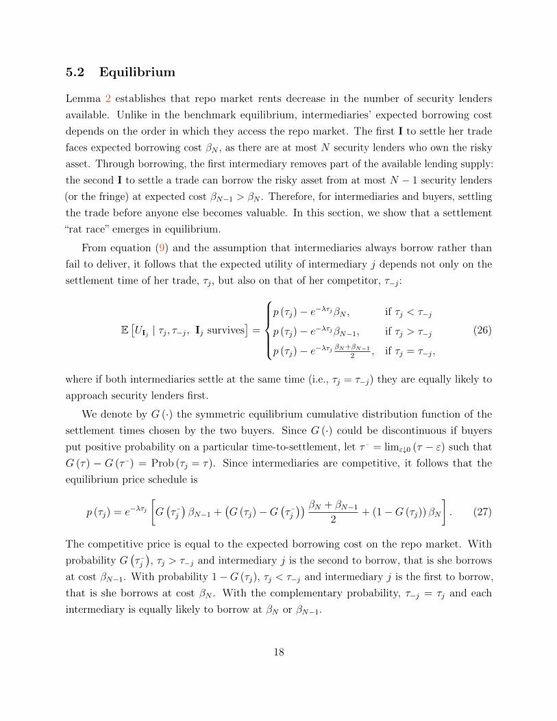
5.2 Equilibrium

Lemma 2 establishes that repo market rents decrease in the number of security lenders

available. Unlike in the benchmark equilibrium, intermediaries’ expected borrowing cost

depends on the order in which they access the repo market. The first I to settle her trade

faces expected borrowing cost βN , as there are at most N security lenders who own the risky

asset. Through borrowing, the first intermediary removes part of the available lending supply:

the second I to settle a trade can borrow the risky asset from at most N − 1 security lenders

(or the fringe) at expected cost βN−1 > βN . Therefore, for intermediaries and buyers, settling

the trade before anyone else becomes valuable. In this section, we show that a settlement

“rat race” emerges in equilibrium.

From equation (9) and the assumption that intermediaries always borrow rather than

fail to deliver, it follows that the expected utility of intermediary j depends not only on the

settlement time of her trade, τj, but also on that of her competitor, τ−j:

E[UIj | τj, τ−j, Ij survives

]=

p (τj)− e−λτjβN , if τj < τ−j

p (τj)− e−λτjβN−1, if τj > τ−j

p (τj)− e−λτj βN+βN−1

2, if τj = τ−j,

(26)

where if both intermediaries settle at the same time (i.e., τj = τ−j) they are equally likely to

approach security lenders first.

We denote by G (·) the symmetric equilibrium cumulative distribution function of the

settlement times chosen by the two buyers. Since G (·) could be discontinuous if buyers

put positive probability on a particular time-to-settlement, let τ− = limε↓0 (τ − ε) such that

G (τ) − G (τ−) = Prob (τj = τ). Since intermediaries are competitive, it follows that the

equilibrium price schedule is

p (τj) = e−λτj[G(τ−j)βN−1 +

(G (τj)−G

(τ−j)) βN + βN−1

2+ (1−G (τj)) βN

]. (27)

The competitive price is equal to the expected borrowing cost on the repo market. With

probability G(τ−j), τj > τ−j and intermediary j is the second to borrow, that is she borrows

at cost βN−1. With probability 1−G (τj), τj < τ−j and intermediary j is the first to borrow,

that is she borrows at cost βN . With the complementary probability, τ−j = τj and each

intermediary is equally likely to borrow at βN or βN−1.

18

Definition 2. (Benchmark utilities.) Let VN (τ) denote the expected utility of each buyer

if the repo borrowing cost for competitive intermediaries is fixed at βN , and let τN be the

optimal settlement time that maximizes VN (τ):

VN (τ) ≡ E [UB | borrowing cost is βN ] = e−δτ(θ − e−λτβN

)and

τN ≡ arg maxτ

VN (τ) = max

0,

1

λlog

[(δ + λ)

θδβN

]. (28)

The benchmark utilities and corresponding optimal settlement delays are equivalent to

those in Section 3 for N > 0. It immediately follows from Lemma 2 that VN (τ) > VN−1 (τ)

for all τ ≥ 0 and that τN ≤ τN−1, with equality only if τN = τN−1 = 0. The intuition is the

same as in the benchmark equilibrium: buyers are overall better off, and would optimally

settle faster, when borrowing costs for the intermediary are lower.

From equations (5), (27), and using Definition 2, we can write the expected buyer utility

as a linear combination of benchmark utilities, that is

E[UBj

]= G

(τ−j)VN−1 (τ)+

(G (τj)−G

(τ−j)) VN (τ) + VN−1 (τ)

2+(1−G (τj))VN (τ) . (29)

Lemma 3. (Buyers’ strategy) If VN−1 (0) + VN (0) ≥ 2VN−1 (τN−1), both buyers choose

immediate settlement with probability π = 1.

If VN−1 (0)+VN (0) < 2VN−1 (τN−1), buyers choose immediate settlement with probability

π < 1, where

π = max

0, 2

VN (0)− VN−1 (τN−1)

VN (0)− VN−1 (0)

. (30)

With probability 1 − π, each buyer chooses a random settlement time in [τ , τN−1] where

τ < τN is pinned down by:

VN−1 (τN−1) = (1− π)VN (τ) + πVN−1 (τ) , (31)

such that the buyer’s expected utility is VN−1 (τN−1).

From Lemma 3, two types of equilibria emerge depending on the model parameters: an

immediate-settlement equilibrium and a delayed-settlement equilibrium. In the immediate-

settlement equilibrium, buyers choose the pure strategy τ ? = 0 and intermediaries always

19

enter repo contracts with security lenders. From equation (27), the price p (0) reflects the

average cost of borrowing, that is,

p (0) =1

2(βN + βN−1) . (32)

In the delayed-settlement equilibrium, buyers randomize over possible times-to-settlement,

using the cumulative distribution function

G (τ) =

π, if τ ∈ [0, τ)

VN (τ)−VN−1(τN−1)

VN (τ)−VN−1(τ), if τ ∈ [τ , τN−1]

1, if τ > τN−1.

(33)

A settlement “rat race” emerges in which each buyer chooses a short settlement delay, so that

his trade is more likely to be settled first. Note that, from equation (28), a settlement delay

choice τ > τN−1 is always sub-optimal for buyers. Therefore, by choosing τN−1 a buyer is sure

to be the second to settle his trade. This pins down the equilibrium utility: In any mixed

strategy (i.e., delayed settlement) equilibrium, buyers earn VN−1 (τN−1).

Mixed strategies in the delayed-settlement equilibrium do not necessarily have a continuous

support. If VN (0) > VN−1 (τN−1), a buyer can improve his utility if he unilaterally deviates

and chooses immediate settlement. In this case, in equilibrium buyers put positive weight

π > 0 on τ ? = 0. With probability 1− π, buyers optimally mix over settlement delays in the

support [τ , τN−1], where τ > 0. Otherwise, if VN (0) ≤ VN−1 (τN−1), buyers use a continuous

mixed strategy such that no time-to-settlement τ is chosen with positive probability.

The expected utility for buyers, across both the immediate- and delayed-settlement

equilibria is therefore

E [UB] = maxVN−1 (τN−1)︸ ︷︷ ︸

delayed-settlementequilibrium

,1

2[VN (0) + VN−1 (0)]

︸ ︷︷ ︸immediate-settlement

equilibrium

. (34)

Figure 3 illustrates the buyers’ strategy G (τ) in the delayed-settlement equilibrium for

different levels of counterparty risk. Intuitively, higher counterparty risk and lower asset

specialness lead to shorter settlement delays in equilibrium.

[ insert Figure 3 here ]

20

Proposition 2 formally states the equilibrium of the trading game for N ≥ 2.

Proposition 2. (Equilibrium, exogenous penalties) If N ≥ 2 and the late-delivery penalty

z is sufficiently large such that (BC) is always true, then the following strategies form an

equilibrium:

(i) Intermediaries post τ, p (τ) contract schedules with τ ≥ 0 and p (τ) as defined in

equation (27), where the equilibrium G (τ) is given in equation (33).

(ii) If VN−1 (0) + VN (0) ≥ 2VN−1 (τN−1), buyers choose immediate settlement (τ ? = 0).

Otherwise, buyers choose a random time-to-settlement from the equilibrium cumulative

distribution G (τ) defined in equation (33).

(iii) Securities lenders mix over repo purchasing prices `. The first and second lender

to be approached by an intermediary draws from distribution FN (`) and FN−1 (`),

respectively, defined in Lemma 1.

(iv) Intermediaries always borrow the asset at settlement time if the large seller did not

arrive before settlement.

Figure 4 illustrates the equilibrium price-settlement delay schedules posted by intermedi-

aries. Everything else equal, a longer time-to-settlement corresponds to a lower probability of

costly borrowing, and therefore to a lower price. The price-settlement delay schedule shifts

up as specialness increases (i.e., for lower ϕ), since security lenders are able to extract higher

rents and increase the expected borrowing cost for intermediaries. Figure 4 also differentiates

between the τ, p (τ) pairs on and off the equilibrium path, that is, the settlement times

buyers choose in equilibrium from the competitive schedule.

[ insert Figure 4 here ]

Corollary 2 states that as the intermediary default rate δ increases, buyers are more

likely to choose immediate settlement. There is a smooth transition between delayed- and

immediate-settlement equilibria for a positive default rate threshold δ, such that buyers choose

immediate settlement with probability one if and only if the default rate of the intermediary

is higher than the threshold.

21

Corollary 2. (Immediate settlement probability) The immediate settlement probability π

weakly increases in the default rate δ. Moreover, there exists a unique default rate threshold

δ > 0 such that for δ < δ the delayed-settlement equilibrium obtains and for δ ≥ δ the

immediate-settlement equilibrium obtains.

We can measure the cost of the settlement rat race for buyers by comparing their

equilibrium expected utility in (34) with a benchmark utility. The rat race emerges either if

buyers trade simultaneously at t = 0, or they cannot observe each other’s choices, or both.

Therefore, a natural utility benchmark is to consider the optimal choices buyers would make

if they arrive sequentially rather than simultaneously, that is τN and τN−1. Let

C = VN (τN) + VN−1 (τN−1)︸ ︷︷ ︸benchmark utility

−max 2VN−1 (τN−1) , VN (0) + VN−1 (0)︸ ︷︷ ︸equilibrium buyers’ utility

(35)

be a measure of the settlement rat race cost for the buyers. Importantly, since borrowing has

a real economic cost (intermediary’s shadow cost of capital), the settlement rat race cost for

the buyers exceeds any additional rents for security lenders due to the higher likelihood of

borrowing.

Corollary 3. (Settlement rat race cost.) The settlement rat race cost C increases in

default risk (δ) and decreases in asset specialness (increases in ϕ) if the delayed-settlement

equilibrium obtains, and decreases in δ and increases in asset specialness (decreases in ϕ)

if the immediate-settlement equilibrium obtains.

A higher default risk has two effects on the settlement race cost. First, the benchmark

optimal settlement time in equation (28) decreases in the default rate δ. Second, from

Corollary 2, the settlement race is reinforced as buyers choose faster settlement. For low

default risk, the delayed-settlement equilibrium obtains and the second effect dominates, that

is, the rat race escalates faster than the corresponding drop in optimal settlement times.

Consequently, the cost of the race increases in counterparty risk. For high default risk, the

immediate settlement equilibrium obtains. In the immediate-settlement equilibrium, a higher

counterparty risk reduces the distance between the optimal time-to-settlement in equation

(28) and the equilibrium choice τ ? = 0. In this case, only the first channel is relevant as

buyers cannot settle trades any faster. Therefore, in the immediate-settlement equilibrium,

the cost of the rat race decreases in counterparty risk δ. A similar reasoning applies when we

consider asset specialness (and, implicitly, borrowing costs) rather than counterparty risk.

22

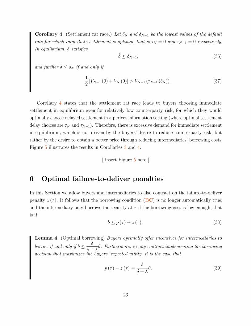
Corollary 4. (Settlement rat race.) Let δN and δN−1 be the lowest values of the default

rate for which immediate settlement is optimal, that is τN = 0 and τN−1 = 0 respectively.

In equilibrium, δ satisfies

δ ≤ δN−1, (36)

and further δ ≤ δN if and only if

1

2[VN−1 (0) + VN (0)] > VN−1 (τN−1 (δN)) . (37)

Corollary 4 states that the settlement rat race leads to buyers choosing immediate

settlement in equilibrium even for relatively low counterparty risk, for which they would

optimally choose delayed settlement in a perfect information setting (where optimal settlement

delay choices are τN and τN−1). Therefore, there is excessive demand for immediate settlement

in equilibrium, which is not driven by the buyers’ desire to reduce counterparty risk, but

rather by the desire to obtain a better price through reducing intermediaries’ borrowing costs.

Figure 5 illustrates the results in Corollaries 3 and 4.

[ insert Figure 5 here ]

6 Optimal failure-to-deliver penalties

In this Section we allow buyers and intermediaries to also contract on the failure-to-deliver

penalty z (τ). It follows that the borrowing condition (BC) is no longer automatically true,

and the intermediary only borrows the security at τ if the borrowing cost is low enough, that

is if

b ≤ p (τ) + z (τ) . (38)

Lemma 4. (Optimal borrowing) Buyers optimally offer incentives for intermediaries to

borrow if and only if b ≤ δ

δ + λθ. Furthermore, in any contract implementing the borrowing

decision that maximizes the buyers’ expected utility, it is the case that

p (τ) + z (τ) =δ

δ + λθ. (39)

23

The result is intuitive. Since intermediaries are competitive, it is the buyers who ultimately

bear the borrowing cost. If intermediaries do not borrow at τ , buyers bear additional

counterparty risk instead: with probability δδ+λ

, the intermediary defaults before the large

seller arrival. Proposition 3 states the equilibrium in the trading game with endogenous

failure-to-deliver penalties.

Proposition 3. (Equilibrium, endogenous penalty.) If buyers and intermediaries can

contract on failure-to-deliver penalties, then the following strategies form an equilibrium:

(i) Intermediaries offer payment and penalty schedules such that

p (τ) = e−λτE[min

b,

δ

δ + λθ

], (40)

z (τ) =δ

δ + λθ − e−λτE

[min

b,

δ

δ + λθ

], (41)

where the closed form expression for E[min

b, δ

δ+λθ]

is given in equation (B.54)

in the Appendix.

(ii) Buyers choose immediate settlement.

(iii) Securities lenders mix over repo purchasing prices `. The first and second lender

to be approached by an intermediary draws from a (generalized) distribution F genN (`)

and F genN−1 (`), defined in equation (B.52) in the Appendix. They charge at most

`gen

=1

R

(min

Γ

2σ2 (R− 1) ,

δ

δ + λθ

+γσ2

2

). (42)

(iv) Intermediaries only borrow the asset if b ≤ δ

δ + λθ.

First, equilibrium price and penalty schedules have an option-like structure. In particular,

the failure-to-delivery penalty resembles a put option on the repo market conditions, with a

strike price equal to the additional counterparty risk for the buyer if the intermediary does not

borrow, that is δδ+λ

θ. We can think of the optimal penalty as insurance against high borrowing

costs on the repo market. Figure 6 illustrates that the equilibrium penalty schedule z (τ)

increases in settlement time and decreases in asset specialness. Intermediaries are optimally

penalized more for a settlement failure if the settlement cycle is long. This is intuitive: since

24

the price p (τ) decreases with the settlement delay, the failure-to-deliver penalty needs to

increase to preserve incentives to borrow. Further, for special assets with high borrowing

costs, buyers optimally offer intermediaries lower incentives to borrow. Consequently, the

failure-to-deliver penalty is lower if the asset supply is more limited.

[ insert Figure 6 here ]

Second, we note that buyers always choose immediate settlement (i.e., τ ? = 0) if they can

contract on failure-to-deliver penalties. The price p (τ) in equation (40) is lower for any τ

than the additional counterparty risk the buyer bears if the intermediary does not borrow,δ

δ+λθ. Therefore, buyers have no incentive to delay settlement in order to avoid borrowing

costs.

To further analyze the equilibrium outcomes, we distinguish between three possible

scenarios. Depending on the relative magnitude of the borrowing costs and the counterparty

risk incurred after the contract settlement time, either (i) δδ+λ

θ ≤ γ2σ2 (R− 1) and borrowing

is never optimal, (ii) δδ+λ

θ > Γ2σ2 (R− 1) and borrowing is always optimal, or (iii) δ

δ+λθ ∈(

γ2σ2 (R− 1) , Γ

2σ2 (R− 1)

]and borrowing may be optimal or not.

Pass-through contracts. First, let δδ+λ

θ ≤ γ2σ2 (R− 1). If counterparty risk is low enough,

or costs of borrowing from perfectly competitive lenders are relatively high, it is optimal for

B that I never borrows. Buyers always choose immediate settlement and, consequently, all

trades (technically) fail to deliver. A pass-through contract emerges, in which no cash changes

hands on the equilibrium path: I simply delivers the asset to B immediately after buying it

from the large seller. From Proposition 3, the equilibrium penalty is zero, that is z (0) = 0:

the intermediary is not penalized for late delivery. While the payment p (τ) is greater than

zero, the intermediary is never able to deliver on time, so the payment is off the equilibrium

path.

Always-borrow contracts. Second, let δδ+λ

θ > Γ2σ2 (R− 1). If counterparty risk is

high enough, or borrowing costs from fringe traders are relatively low, it is optimal for B

that I always borrows. We recover the equilibrium in Section 5, for π = 1. In addition,

the equilibrium contract specifies a penalty schedule z (τ) as in (41). However, since the

intermediary always borrows, paying the late delivery penalty is not on the equilibrium path.

25

Random fails-to-deliver. If δδ+λ

θ ∈(γ2σ2 (R− 1) , Γ

2σ2 (R− 1)

], then the buyer would

like to offer incentives to the intermediary to borrow from the N security lenders, but not

from the fringe lenders. The N security lenders still earn rents, but lower – as the “reservation

cost” of the intermediary changes. A trade fails to settle with probability (1− ϕ)N , that is if

none of the N security lenders own the asset.

Figure 7 illustrates the failure-to-deliver probability as a function of asset specialness for

all three scenarios.

[ insert Figure 7 here ]

Unlike in Section 5, the repo prices depend on the counterparty risk level. Figure 8

illustrates rents for a security lender, conditional on owning the asset, as a function of

counterparty risk.

[ insert Figure 8 here ]

Repo prices increase in counterparty risk, since the upper bound on the intermediaries’

borrowing cost increases in δ. Therefore, for larger counterparty risk, lenders are better able

to hold up intermediaries and extract rents from them.

Discussion of zero-penalty contracts. Our analysis in Sections 4 through 6 focuses on

either “large enough” or flexible failure-to-deliver penalties. Another possible case would

be a zero or “low enough” penalty. From the discussion above, a zero penalty emerges in

equilibrium if δδ+λ

θ ≤ γ2σ2 (R− 1), that is for the pass-through contracts. Otherwise, a

zero-penalty contract leads to either rents for intermediaries, sub-optimal security borrowing

decisions, or both. If buyers can choose both a price upon successful delivery and a penalty

upon failure-to-deliver, they can simultaneously achieve two objectives, that is (i) implement

the incentive-compatible repo borrowing choice in Lemma 4 and also (ii) extract the full

trading surplus from the intermediary. A zero failure-to-deliver penalty implies buyers have a

single tool (i.e., price upon successful delivery) to implement both objectives. Therefore, since

buyers cannot penalize intermediaries ex-post, they must increase the price to offer higher

borrowing incentives, allowing intermediaries to extract rents. However, since buyers never

pay a price higher than the additional counterparty risk δδ+λ

θ, they will still optimally choose

immediate settlement even if penalties are zero. The rationale is the same as in Proposition 3.

26

7 Conclusions

This paper provides insights into the consequences of changing the rules for trade settlement

on financial markets. The current settlement process, involving several days of delay between

trade and settlement, feels at odds with the fast-paced markets of today. Both market

participants and financial regulators agree on this. Further, new technologies such as

distributed ledgers and smart contracts can offer traders the flexibility to fine-tune settlement

cycles on a trade-by-trade or asset-by-asset basis.

We emphasize three insights emerging from our results. First, flexible settlement cycles

allow traders to individually balance counterparty risk and borrowing costs on the securities

loan market.

Second, high failure-to-deliver penalties are not necessarily a panacea for market quality

as they lead to excessive security borrowing. Imperfect competition between security lenders

generates a strong incentive to settle trades before everyone else. In an attempt to reduce

borrowing costs, traders engage in a settlement rat race. In equilibrium, there is excess

demand for fast, or even immediate, settlement. Security lenders earn high rents at the

expense of traders, and welfare is reduced.

Finally, we find that the optimal trade contract combines flexible failure-to-deliver penalties

with immediate settlement. The equilibrium penalty resembles a put option on the repo

market, and it serves a double purpose: First, it provides insurance for traders against high

borrowing costs. Second, it improves welfare by fostering competition on the security lending

market.

27

References

Acharya, Viral, and Alberto Bisin, 2014, Counterparty risk externality: Centralized versus

over-the-counter markets, Journal of Economic Theory 149, 153–182.

Acharya, Viral V., 2009, Centralized clearing for credit derivatives, in Restoring Financial

Stability, pp. 251–268.

Aune, Rune, Maureen O’Hara, and Ouziel Slama, 2017, Footprints on the blockchain:

Information leakage in distributed ledgers, Working paper.

BCG, 2012, Shortening the Settlement Cycle, Discussion paper, Boston Consulting Group.

Benos, Evangelos, Rod Garratt, and Pedro Gurrola-Perez, 2017, The economics of Distributed

Ledger Technology for securities settlement, Bank of England Staff Working paper No. 670.

Biais, Bruno, Christophe Bisiere, Matthieu Bouvard, and Catherine Casamatta, 2018, The

blockchain folk theorem, Toulouse School of Economics Working paper No. 17–817.

Brainard, Lael, 2016, Distributed ledger technology: Implications for payments, clearing, and

settlement, Board of Governors of the Federal Reserve System Speech.

Chague, Fernando, Rodrigo De-Losso, Alan De Genaro, and Bruno Giovannetti, 2017, Well-

connected short-sellers pay lower loan fees: A market-wide analysis, Journal of Financial

Economics 123, 646 – 670.

Cong, Lin William, and Zhiguo He, 2018, Blockchain disruption and smart contracts, Working

paper.

Corradin, Stefano, and Angela Maddaloni, 2017, The importance of being special: Repo

markets during the crisis, ECB Working paper No. 2065.

D’Avolio, Gene, 2002, The market for borrowing stock, Journal of Financial Economics 66,

271 – 306.

Duffie, Darrell, 1996, Special repo rates, The Journal of Finance 51, 493–526.

, Nicolae Garleanu, and Lasse Heje Pedersen, 2002, Securities lending, shorting, and

pricing, Journal of Financial Economics 66, 307 – 339.

28

Duffie, Darrell, and Haoxiang Zhu, 2011, Does a central clearing counterparty reduce counter-

party risk?, Review of Asset Pricing Studies 1, 74–95.

ECB, 2016, Distributed ledger technology, Discussion paper, European Central Bank.

ESMA, 2016, The distributed ledger technology applied to securities markets, Discussion

paper, European Securities and Markets Authority.

Evans, Richard B., Rabih Moussawi, Michael S. Pagano, and John Sedunov, 2017, Etf

failures-to-deliver: Naked short-selling or operational shorting?, Working paper.

Fleming, Michael J., and Kenneth Garbade, 2005, Explaining settlement fails, Current Issues

in Economics and Finance 11.

Foley-Fisher, Nathan, Stefan Gissler, and Stephane Verani, 2017, Over-the-counter market

liquidity and securities lending, Working paper.

Fotak, Veljko, Vikas Raman, and Pradeep K. Yadav, 2014, Fails-to-deliver, short selling, and

market quality, Journal of Financial Economics 114, 493–516.

Geczy, Christopher C., David K. Musto, and Adam V. Reed, 2002, Stocks are special too: an

analysis of the equity lending market, Journal of Financial Economics 66, 241 – 269.

Grossman, Sanford J., and Merton H. Miller, 1988, Liquidity and market structure, The

Journal of Finance 43, 617–633.

Huszar, Zsuzsa R., and Zorka Simon, 2018, The pricing implications of oligopolistic securities

lending market: A beneficial owner perspective, Netspar Working paper DP 09/2017-032.

IHS Markit, 2016, Securities Lending: Year in Review, Discussion paper, IHS Markit.

Janssen, Maarten, and Eric Rasmusen, 2002, Bertrand competition under uncertainty, The

Journal of Industrial Economics 50, 11–21.

Jordan, Bradford D., and Susan D. Jordan, 1997, Special repo rates: An empirical analysis,

The Journal of Finance 52, 2051–2072.

Jovanovic, Boyan, and Albert J. Menkveld, 2017, Dispersion and skewness of bid prices,

Working paper.

29

Koeppl, Thorsten, and Jonathan Chiu, 2018, Blockchain-based settlement for asset trading,

Queen’s Economics Department Working paper No. 1397.

Kyle, Albert S., and Anna A. Obizhaeva, 2017, Market microstructure invariance: A dynamic

equilibrium model, Working paper.

Levitt, Arthur, 1996, Speeding up settlement: The next frontier, Symposium on Risk Reduction

in Payments, Clearance, and Settlement Systems.

Loon, Yee Cheng, and Zhaodong Ken Zhong, 2014, The impact of central clearing on

counterparty risk, liquidity, and trading: Evidence from the credit default swap market,

Journal of Financial Economics 112, 91–115.

Malinova, Katya, and Andreas Park, 2017, Market design for trading with blockchain

technology, Working paper.

Menkveld, Albert J, 2017, Crowded positions: An overlooked systemic risk for central clearing

parties, The Review of Asset Pricing Studies 7, 209–242.

Pirrong, Craig, 2009, The economics of clearing in derivatives markets: netting, asymmetric

information, and the sharing of default risks through a central counterparty, Working paper.

Saleh, Fahad, 2017, Blockchain without waste: Proof-of-stake, Working paper.

Stephens, Eric, and James R. Thompson, 2017, Information asymmetry and risk transfer

markets, Journal of Financial Intermediation 32, 88 – 99.

Tobias, Adrian, Brian Begalle, Adam Copeland, and Antoine Martin, 2013, Risk Topography:

Systemic Risk and Macro Modeling; chap. Repo and Securities Lending, pp. 131–148.

30

A Notation summary

Model parameters and their interpretation.

Parameter Definition

σ Asset volatility.δ Intermediary default rate.λ Large seller arrival rate.θ Buyer private value for the asset.γ,Γ Risk-aversion of security lenders, with γ < Γ.N Number of security lenders with risk aversion γ.ϕ Probability a security lender owns the asset.R Opportunity cost of collateral for intermediary.

B Proofs

Proposition 1

Proof. The proof follows immediately from the discussion in the main text. For (i), equation(15) pins down the competitive price for intermediaries.

The optimal settlement time in (ii) solves the first order condition

∂E [UB]

∂τ= 0, (B.1)

where E [UB] is given in equation (16). It follows that:

∂E [UB]

∂τ= e−τ(δ+λ)

[Γ

2(R− 1)σ2 (δ + λ)− δθeλτ

], (B.2)

and therefore τ ? = max

0, 1λ

log[

(δ+λ)θδ

Γ2σ2 (R− 1)

], that is the expression in equation (17).

The security lenders competitive prices in (iii), that is ` = Γ2σ2, follow from (10) holding

with equality. Finally, by assumption, the penalty is high enough such that the intermediaryalways borrows the asset at τ ? if she does not own it.

Corollary 1

Proof. Let’s introduce an auxiliary variable

τ =1

λlog

[(δ + λ)

θδ

Γ

2σ2 (R− 1)

](B.3)

31

so that τ ? = max 0, τ. We take the partial derivatives of τ with respect to all the parametersand sign them to establish monotonicity, that is

(∂τ

∂Γ,∂τ

∂σ,∂τ

∂R,∂τ

∂δ,∂τ

∂θ

)=( 1

Γλ︸︷︷︸>0

,2

σλ︸︷︷︸>0

,1

λ (R− 1)︸ ︷︷ ︸>0

,− 1

δ (δ + λ)︸ ︷︷ ︸<0

,− 1

θλ︸︷︷︸<0

). (B.4)

The partial derivative of τ with respect to the large seller’s arrival rate λ is

∂τ

∂λ=

1

λ2

[λ

δ + λ− log

(Γ(R− 1)σ2(δ + λ)

2δθ

)]. (B.5)

Define a function f as

f (λ, ·) =λ

δ + λ− log

(Γ(R− 1)σ2(δ + λ)

2δθ

). (B.6)

Since 1λ2 is positive, it follows that the sign of ∂τ

∂λis the same as the sign of f (λ, ·). First, we

note that f (λ, ·) decreases in λ since

∂f (λ, ·)∂λ

= − λ

(λ+ δ)2 < 0. (B.7)

Second, we compute the limits of f (λ, ·), that is:

limλ→0

f (λ, ·) = log(θ)− log

(Γ

2σ2(R− 1)

)and (B.8)

limλ→∞

f (λ, ·) = −∞. (B.9)

Since θ > Γ2σ2(R− 1), limλ→0 f (λ, ·) > 0. Then since f (λ, ·) is monotonous it follows that

there exists a unique Λ0 > 0 such that τ increases in λ for λ ≤ Λ0 and τ decreases in λ forλ > Λ0.

Lemma 1

Proof. First, there are no prices ` such that a lender offers a given ` with positive probability.From Janssen and Rasmusen (2002 pp. 12-13), either `+ ε or `− ε with ε sufficiently close tozero would represent a profitable deviation.

In a mixed strategy equilibrium, lenders are indifferent between all prices in the support,that is the following first-order condition is true:

∂E [UL (`)]

∂`= 0. (B.10)

32

From (B.10) and equation (21), the cumulative distribution function FN (·) solves thedifferential equation:

− 1

2ϕ [1− ϕFN(`)]N−2 [(N − 1)ϕF ′N(`)

(2`− γσ2

)+ 2ϕFN(`)− 2

]= 0, (B.11)

subject to the boundary condition FN(`)

= 1 where from (20), ` = Γ2σ2 − Γ−γ

2Rσ2.

The corresponding partial equilibrium mixed strategy is:

FN (`) =

0, if ` ≤ `

ϕ−1[1− (1− ϕ) N−1

√σ2(R−1)(Γ−γ)R(2`−γσ2)

], if ` ∈

(`, `]

1, if ` ≥ `.

(B.12)

and ` = σ2

2

[γ + (Γ− γ) R−1

R(1− ϕ)N−1

]such that FN (`) = 0.

The lender is indifferent between all prices in the support. If he asks for the maximumprice `, L only makes a profit if no other lender owns the asset. Consequently, the expectedutility for L is:

E [UL] = ϕ (1− ϕ)N−1(`− γ

2σ2)

= ϕ (1− ϕ)N−1 σ2

2(Γ− γ)

R− 1

R. (B.13)

Lemma 2

Proof. The cumulative distribution function of mini=1,...,k `i, if k lenders own the asset, is

1− (1− FN (`))k. Since k itself is random, we can write the expectation of mini `i − γ2σ2 if at

least one lender owns the asset (that is, if 1ΩL 6=∅ = 1) as:

E[mini

(`i −

γ

2σ2)1ΩL 6=∅

]

=

∫ `

`

N∑

k=1

(Nk

)ϕk (1− ϕ)N−k

(`− γ

2σ2)k (1− FN (`))k−1 dFN (`)

=

∫ `

`

Nϕ (1− ϕFN (`))N−1(`− γ

2σ2)

dFN (`)

= Nϕ (1− ϕ)N−1 σ2

2(Γ− γ)

R− 1

R, (B.14)

where the last line follows from the lender being indifferent between all prices in[`, `].

33

It further follows that

E[mini`i | ΩL 6= ∅

]=N σ2

2(Γ− γ) R−1

Rϕ (1− ϕ)N−1

1− (1− ϕ)N+γ

2σ2. (B.15)

Therefore, after replacing (B.15) in (24) it follows that

βN =σ2

2(R− 1)

[γ + (Γ− γ)

[Nϕ (1− ϕ)N−1 + (1− ϕ)N

]]. (B.16)

The partial derivative of βN with respect to N is

∂βN∂N

=σ2

2(R− 1) (Γ− γ) (1− ϕ)N−1

︸ ︷︷ ︸>0

[ϕ+ (1 + ϕ (N − 1)) log (1− ϕ)] . (B.17)

We study the sign of g (N) ≡ ϕ+ (1 + ϕ (N − 1)) log (1− ϕ). First, note that

∂g (N)

∂N= ϕ log (1− ϕ) ≤ 0, (B.18)

since ϕ ∈ [0, 1]. Therefore g (N) weakly decreases in N . Further, g (1) = ϕ+ log (1− ϕ) ≤ 0

for any ϕ ∈ [0, 1] since ∂(ϕ+log(1−ϕ))∂ϕ

= ϕϕ−1

< 0 and ϕ+ log (1− ϕ) = 0 for ϕ = 0. It follows

that g (N) < 0 for any N ≥ 1. Consequently, ∂βN∂N

< 0 and the expected borrowing cost βNdecreases in N for ϕ ∈ (0, 1].

The partial derivative of βN with respect to ϕ is

∂βN∂ϕ

= − σ2

2(R− 1) (Γ− γ) (1− ϕ)N−2 ϕN (N − 1)

︸ ︷︷ ︸>0

< 0, (B.19)

and therefore the expected borrowing cost βN decreases in ϕ.

Lemma 3

Proof.

Sublemma B.1. Buyers never choose τ > τN−1.

Proof. Since τN−1 > τN , VN (τN−1) > VN (τ) for all τ > τN−1. Therefore, from the definitionof τN−1, for any α ∈ [0, 1],

αVN (τN−1) + (1− α)VN−1 (τN−1) > αVN (τ) + (1− α)VN−1 (τ) ,∀τ > τN−1. (B.20)

It follows that deviations from τ > τN−1 to τN−1 are profitable for any probability of beingthe first to settle the trade.

34

Sublemma B.2. If 12

[VN (0) + VN−1 (0)] ≥ VN−1 (τN−1), then(τ ?j , τ

?−j)

= (0, 0) is a purestrategy equilibrium.

Proof. If both buyers choose immediate settlement, they are equally likely to settle first orsecond, and have expected utility 1

2(VN (0) + VN−1 (0)). If any buyer unilaterally deviates

to τ > 0, then he is sure to settle after his competitor and can earn at most VN−1 (τN−1).Therefore, no deviation from τ = 0 is profitable.

Sublemma B.3. Buyers never choose a specific τ > 0 with positive probability.

Proof. Assume buyers choose τ ′ > 0 with positive probability η. With probability η2, bothbuyers select τ ′ and earn η2

2(VN (τ ′) + VN−1 (τ ′)). A buyer can increase his expected profit

by putting zero weight on τ ′ and choosing instead τ ′ − ε ≥ 0 with positive probability, for asufficiently small ε. Such deviation increases the expected profit to η2VN (τ ′ − ε).Sublemma B.4. The upper bound of the support for any equilibrium mixed strategy of B, ifsuch a strategy exists, is τN−1.

Proof. Assume there exists an equilibrium mixed strategy with cumulative distributionfunction G (τ). Further, assume τ 6= τN−1 is the smallest time-to-settlement such thatG (τ) = 1, that is the upper bound of the mixed strategy support. From Sublemma B.1 itmust be that τ < τN−1. If a buyer chooses τ , he is sure to be the second to settle and obtainVN−1 (τ). If the buyer instead deviates to τN−1, since G (τN−1) = 1, he also is the second tosettle but obtains the higher utility level VN−1 (τN−1) > VN−1 (τ) (by the definition of τN−1).Therefore, it must be that τ = τN−1.

Corollary B.1. If there exists an equilibrium mixed strategy for B, it yields expected utilityVN−1 (τN−1).

Proof. From Sublemma B.4, if an equilibrium mixed strategy exists, then τN−1 is in themixing support and further G (τN−1) = 1. Therefore, by choosing τN−1 a buyer is guaranteedto be second to settle his trade and earns expected utility VN−1 (τN−1), which is necessarilythe expected utility of any other time-to-settlement in the mixed strategy support.

Sublemma B.5. If 12

[VN−1 (0) + VN (0)] ≥ VN−1 (τN−1), then(τ ?j , τ

?−j)

= (0, 0) is the uniqueequilibrium.

Proof. From Sublemma B.2,(τ ?j , τ

?−j)

= (0, 0) is a pure strategy equilibrium yielding expected

utility 12

[VN−1 (0) + VN (0)]. Sublemma B.3 further establishes that(τ ?j , τ

?−j)

= (0, 0) is theunique pure strategy equilibrium. It remains to be shown there are no mixed strategyequilibria. If there is one, from Corollary B.1 it yields utility VN−1 (τN−1), which is weaklylower than the utility of the pure strategy equilibrium, that is 1

2[VN−1 (0) + VN (0)]. Therefore,

there can be no mixed strategy equilibrium.

Sublemma B.5 completes the proof for the first part of Lemma 3. In what follows, wediscuss the buyers’ equilibrium strategies if VN−1 (τN−1) > 1

2[VN−1 (0) + VN (0)].

35

Sublemma B.6. If VN−1 (τN−1) > VN (0), then the unique equilibrium is in mixed strategies:buyers randomize between τ and τN−1, where τ solves

VN (τ) = VN−1 (τN−1) . (B.21)

Proof. First off, if VN−1 (τN−1) > VN (0) then since (i) VN (τN) > VN−1 (τN−1), and (ii)VN (τ) increases on [0, τN ], it follows that there exists a strictly positive τ < τN such thatVN (τ) = VN−1 (τN−1).

Second, τ must be the lower bound of any equilibrium mixed strategy support. Assumeinstead τ− < τ is the lower bound. If the buyer chooses τ−, then he is the first to settle andobtains VN (τ−). Since τ < τN , it follows that VN (τ−) < VN(τ) = VN−1 (τN−1), which is theexpected utility of a mixed strategy equilibrium, from Corollary B.1. Assume now τ+ > τ isthe lower bound. A buyer can profitably deviate by choosing τ + ε < τ+, then he is the firstto settle and obtains VN (τ + ε) > VN(τ) = VN−1 (τN−1).

Third, no buyer can profitably deviate to immediate settlement. Choosing τ = 0 ensuresthat a buyer is first to settle and gain VN(0) < VN−1 (τN−1).

If 12

[VN−1 (0) + VN (0)] < VN−1 (τN−1) ≤ VN (0) then:

1. Buyers are better off by playing a mixed strategy yielding expected utility VN−1 (τN−1)than by choosing immediate settlement in pure strategies.

2. However, if the competitor plays such a mixed strategy and chooses a random time tosettlement between τ > 0 and τN−1, then immediate settlement is a profitable deviationas it guarantees being first to settle the trade and yields expected utility VN (0).

It follows that buyers choose immediate settlement with some positive probability π < 1.The expected utility of Bj from choosing τ = 0 is:

E[UBj (τ = 0)

]=π

2[VN−1 (0) + VN (0)]

︸ ︷︷ ︸B−j chooses τ=0

+ (1− π)VN (0)︸ ︷︷ ︸B−j chooses τ>0

. (B.22)

The expected utility from choosing immediate settlement needs to be equal, in equilibrium,with the expected utility of any other settlement time choice in the mixed distribution support.Therefore, π is pinned down by

π

2[VN−1 (0) + VN (0)] + (1− π)VN (0) = VN−1 (τN−1) , (B.23)

and therefore

π = 2VN (0)− VN−1 (τN−1)

VN (0)− VN−1 (0). (B.24)

If a buyer chooses the lower bound of the mixed strategy distribution, τ , then he settles firstwith probability 1− π. Therefore, since all points in the mixed strategy support yield the

36

same expected utility, τ solves

(1− π)VN (τ) + πVN−1 (τ) = VN−1 (τN−1) . (B.25)

Note that the two mixed strategy cases, that is 12

[VN−1 (0) + VN (0)] < VN−1 (τN−1) ≤ VN (0)and VN−1 (τN−1) > VN (0), can be put together if redefine π as

π = max

0, 2

VN (0)− VN−1 (τN−1)

VN (0)− VN−1 (0)

. (B.26)

Proposition 2

Proof. First, equation (27), evaluated at the equilibrium buyer’s strategy G (τ) given in(33), implies that the intermediaries earn zero expected profit if they rationally anticipatethe buyers’ and security lenders’ equilibrium behaviour. Second, Lemma 3 solves for theequilibrium buyers’ strategy given competitive intermediaries and the equilibrium lenders’behaviour. Third, Lemma 1 describes the equilibrium behaviour of security lenders. Finally,we assume intermediaries always borrow the asset at settlement if the large seller did notarrive.

Corollary 2

Proof. From the envelope theorem and τN ≥ 0, VN (τN) decreases in δ since

∂VN (τN)

∂δ= −τNVN (τN) ≤ 0,∀N ≥ 1. (B.27)

From Lemma 3, the immediate settlement probability π weakly decreases in VN−1 (τN−1).Since the immediate settlement value functions VN (0) and VN−1 (0) do not depend on δ, itfollows that the immediate settlement probability π weakly increases in δ.

From Lemma 3, for δ ↓ 0, buyers choose an arbitrarily large time-to-settlement and neverchoose immediate settlement: consequently, π = 0. For δ →∞, both buyers always chooseimmediate settlement, that is π = 1. It follows that there exists a δ such that π = 1 for δ > δ.

Corollary 3

Proof. From Lemma 3, buyers choose immediate settlement with probability one if and onlyif VN−1 (0) + VN (0) ≥ VN−1 (τN−1), which therefore corresponds to the case δ > δ. Thesettlement rat race cost for the buyers is:

C = VN (τN) + VN−1 (τN−1)− (VN (0) + VN−1 (0)) , (B.28)

37

which decreases in δ and since both VN (τN) and VN−1 (τN−1) decrease in δ, while VN (0) andVN (0) do not depend on δ.

Since Lemma 2 establishes βN decreases in ϕ, to show that the cost C in (B.28) decreasesin ϕ it is enough to show that

∂ (VN (τN)− VN (0))

∂βN> 0, (B.29)

for all N and τN > 0. We compute the partial derivative and obtain

∂ (VN (τN)− VN (0))

∂βN= 1−

[βN (δ + λ)

δθ

]− δ+λλ

. (B.30)

Since τN > 0, from Definition 2 it follows that βN (δ+λ)δθ

> 1. Consequently, since δ > 0 and

λ > 0,[βN (δ+λ)

δθ

]− δ+λλ< 1 which implies the partial derivative in (B.29) is positive.

Conversely, if δ < δ, VN−1 (0) + VN (0) < VN−1 (τN−1) and buyers choose immediatesettlement with probability π < 1. The rat race cost is in this case is:

C = VN (τN)− VN−1 (τN−1) . (B.31)

To show the cost increases in δ, it is enough to show that ∂2VN (τN )∂N∂δ

> 0 or, since βN decreases

in N , that ∂2VN (τN )∂βN∂δ

< 0. The latter expression can be written as

∂2VN (τN)

∂βN∂δ=

1

δλ

(βN (δ + λ)

δθ

)− δ+λλ(δ log

[βN (δ + λ)

δθ

]− λ). (B.32)

It remains to be shown that δ log[βN (δ+λ)

δθ

]< λ. Since θ > β0 > βN , it follows that:

log

[βN (δ + λ)

δθ

]< log

(1 +

λ

δ

)<λ

δ, (B.33)

and therefore it follows that ∂2VN (τN )∂βN∂δ

< 0.

To show that the settlement rat race cost increases in ϕ, it is enough to show that∂2VN (τN )∂N∂ϕ

> 0 or, alternatively, that ∂2VN (τN )

∂β2N

> 0 since from Lemma 2 βN decreases in both N

and ϕ. Indeed,

∂2VN (τN)

∂β2N

=δθ

β2Nλ

(βN (δ + λ)

δθ

)− δλ

> 0, (B.34)

which concludes the proof.

38

Corollary 4

Proof. We solve the equations τN = 0 and τN−1 = 0 and obtain

δN ≡λβNθ − βN

≤ λβN−1

θ − βN−1

≡ δN−1, (B.35)

since βN ≤ βN−1 and θ > β0 ≥ βN for any positive N . Clearly, δ < δN−1. Otherwise, forsome δN−1 + ε < δ (with arbitrarily small ε), we have that τN (δN−1 + ε) = τN−1 (δN−1 + ε)=0and consequently:

π = 2VN (0)− VN−1 (0)

VN (0)− VN−1 (0)= 2 > 1, (B.36)

which is a contradiction since π ≤ 1.

For δ < δN , the following condition needs to hold

1

2[VN−1 (0) + VN (0)] > VN−1 (τN−1 (δN)) , (B.37)

since if VN−1 (τN−1 (δN)) ≥ 12

[VN−1 (0) + VN (0)] then from Lemma 3 buyers choose immediate

settlement (π = 1) for δN and therefore δN ≥ δ.

Lemma 4

Proof. Let Ggen (·) denote the generalized equilibrium time-to-settlement mixing distributionif the penalty z (τ) is endogenous. Using the same logic as in equations (26) and (27), andacknowledging the intermediary fails to deliver if the penalty is small enough, the expectedintermediary utility is:

E [UI | I survives] =(1− e−λτ

)p (τ) (B.38)

+ e−λτ (1−Ggen (τ))EN [max p (τ)− b,−z (τ)]+ e−λτGgen (τ−)EN−1 [max p (τ)− b,−z (τ)]

+ e−λτ (Ggen (τ)−Ggen (τ−))1

2

(EN [max p (τ)− b,−z (τ)]

+ EN−1 [max p (τ)− b,−z (τ)]),

where EN [·] denotes expectation conditional on at most N security lenders with risk-aversionγ being available.

We note that the intermediary’s borrowing decision depends on the sum between the priceand the penalty, and we define x (τ) = p (τ) + z (τ). Let αN (τ) = PN (b ≤ x (τ)), that is theprobability that (BC) holds conditional on a given N . It follows that the expected utility of

39

the buyer is

E [UB] = e−δτ(1− e−λτ

)(θ − p (τ)) (B.39)

+ e−(δ+λ)τGgen (τ−)

[αN−1 (τ) (θ − p (τ)) + (1− αN−1 (τ))

(z (τ) +

λ

λ+ δθ

)]

+ (1−Ggen (τ))

[αN (τ) (θ − p (τ)) + (1− αN (τ))

(z (τ) +

λ

λ+ δθ

)]

+1

2(Ggen (τ)−Ggen (τ−))

[αN (τ) (θ − p (τ)) + (1− αN (τ))

(z (τ) +

λ

λ+ δθ

)]

+

[αN−1 (τ) (θ − p (τ)) + (1− αN−1 (τ))

(z (τ) +

λ

λ+ δθ

)].

Combining equations (B.38) and (B.39), we obtain an expression for the buyers’ expectedutility which is qualitatively similar to equation (29), that is

E [UB] =Ggen (τ−)V genN−1 (τ) + (Ggen (τj)−Ggen (τ−))

V genN (τ) + V gen

N−1 (τ)

2+ (1−Ggen (τ))V gen

N (τ) , (B.40)

where V genN (·) is a generalization of VN (·) in (28) as follows:

V genN (τ) = e−δτ

[(1− e−λτ

)θ + e−λτ

(λ

λ+ δθ + αN (τ)

(δ

λ+ δθ − EN [b | b ≤ x (τ)]

))],

(B.41)for x (τ) = p (τ) + z (τ) and for any N ≥ 1.

Next, we show that V genN (τ) reaches its maximum if x (τ) = δ

λ+δθ, for any N , which is

enough to prove the Lemma. Dropping the argument τ for exposition purposes, we want tomaximize:

x? = arg maxx

PN (b ≤ x)

δ

λ+ δθ − E [b | b ≤ x]

. (B.42)

Denote the cumulative distribution of b, conditional on N as HN (·) :[bN , bN

]7→ [0, 1] and

let hN (·) be the density function. We can therefore rewrite (B.42) as

x? = arg maxx

δ

λ+ δθHN (x)−

∫ x

bN

y dHN (y) . (B.43)

From the first order condition, it follows that x? solves

(δ

λ+ δθ − x?

)hN (x?) = 0, (B.44)

and x? = δλ+δ

θ since hN (x) > 0 on the support. Consequently, p (τ) + z (τ) = δλ+δ

θ.

40

Proposition 3

Proof. From equation (9) and Lemma 4 we can rewrite the intermediaries’ expected utilityas:

E [UI | I survives] = p (τ)− e−λτE[min

b,

δ

δ + λθ

]. (B.45)

Since intermediaries are competitive, they earn zero expected utility. Consequently, thecompetitive price and penalty schedules become:

p (τ) = e−λτE[min

b,

δ

δ + λθ

]and (B.46)

z (τ) =δ

δ + λθ − e−λτE

[min

b,

δ

δ + λθ

]. (B.47)

Further, from (B.46) and (B.47), if the optimal penalty schedule is implemented, thebuyers’ expected utility in (5) and (6) is the same irrespective of whether the intermediaryborrows at settlement or not, that is:

E [UB] = e−δτ (θ − p (τ)) . (B.48)

From equations (B.46) and (B.48), the optimal settlement time τ ? is

τ ? = max

0,

1

λlog

((δ + λ)

θδE[min

b,

δ

δ + λθ

]). (B.49)

Since E[min

b, δ

δ+λθ]≤ δ

δ+λθ, it follows that τ ? = 0 and buyers choose immediate settlement

in equilibrium.

Securities lenders charge prices ` such that an intermediary is not better off by (i) borrowingfrom a fringe lender, or (ii) failing to settle and paying the penalty. That is, the upper boundon ` is pinned down by

R`− γ

2σ2 ≤ min

Γ

2σ2 (R− 1) ,

δ

δ + λθ

. (B.50)

The maximum ` security lenders ask for is

`gen

=min

Γ2σ2 (R− 1) , δ

δ+λθ

+ γσ2/2

R. (B.51)

As in Section 5.1, security lenders randomize over repo prices. Following the same stepsas in the proof of Lemma 1, we can solve for the (generalized) equilibrium distribution of

41

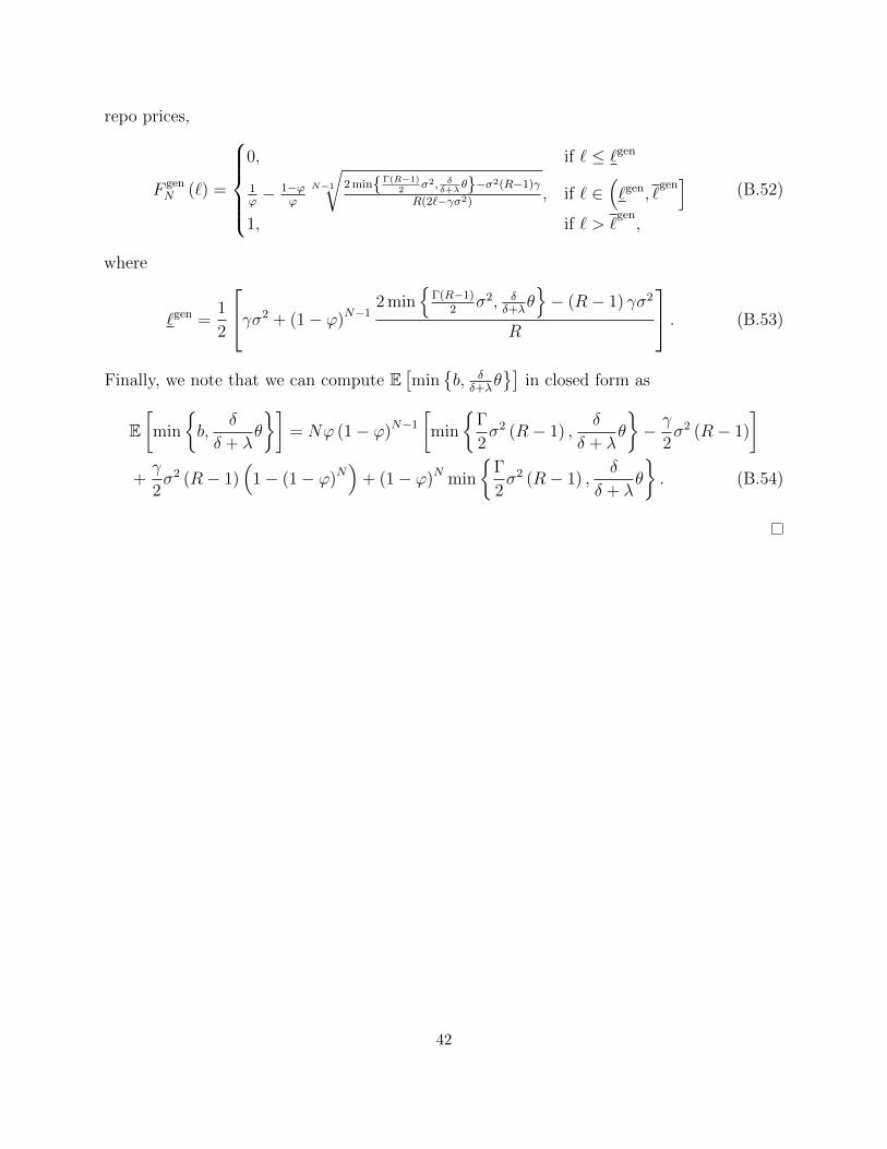
repo prices,

F genN (`) =

0, if ` ≤ `gen

1ϕ− 1−ϕ

ϕ

N−1

√2 minΓ(R−1)

2σ2, δ

δ+λθ−σ2(R−1)γ

R(2`−γσ2), if ` ∈

(`gen, `

gen]

1, if ` > `gen,

(B.52)

where

`gen =1

2

γσ2 + (1− ϕ)N−1

2 min

Γ(R−1)2

σ2, δδ+λ

θ− (R− 1) γσ2

R

. (B.53)

Finally, we note that we can compute E[min

b, δ

δ+λθ]

in closed form as

E[min

b,

δ

δ + λθ

]= Nϕ (1− ϕ)N−1

[min

Γ

2σ2 (R− 1) ,

δ

δ + λθ

− γ

2σ2 (R− 1)

]

+γ

2σ2 (R− 1)

(1− (1− ϕ)N

)+ (1− ϕ)N min

Γ

2σ2 (R− 1) ,

δ

δ + λθ

. (B.54)

42

Figure 1: Benchmark equilibrium time-to-settlement and the corresponding priceThis figure illustrates the equilibrium time-to-settlement and the corresponding trade price asa function of the default rate δ (top panel) and the large seller’s arrival rate λ (bottom panel).Parameter values: σ = 1, θ = 2, Γ = 2, R = 2, λ = 0.5 (top panel), and δ = 0.2 (bottom panel).

0.0 0.2 0.4 0.6 0.8 1.0Intermediary default rate, δ

0

2

4

6

8

10

Tim

e-to

-set

tlem

ent

Immediate settlement (τ ? = 0)

δ = λ(θβ−1

0 − 1)−1

0.0

0.2

0.4

0.6

0.8

1.0

Pric

e

Equilibrium time-to-settlement (τ ?)B-I trade price p(τ ?)

(a) Time-to-settlement, trade price, and counterparty risk.

0.0 0.5 1.0 1.5 2.0 2.5 3.0Large seller arrival rate, λ

0.0

0.2

0.4

0.6

0.8

1.0

1.2

Tim

e-to

-set

tlem

ent

λ = δ(θβ−1

0 − 1)

0.2

0.4

0.6

0.8

1.0

Pric

e

Equilibrium time-to-settlement (τ ?)B-I trade price p(τ ?)

(b) Time-to-settlement, trade price, and seller arrival rate.

43

Figure 2: Competition and borrowing costs on the repo marketPanel (a) illustrates the comparative statics of the distribution of repo prices, FN (`), with respectto the number of lenders, N , and the probability that each lender owns the security, ϕ, which werefer to as asset specialness. A lower ϕ corresponds to a higher specialness. Panel (b) illustratesthe expected borrowing cost for the intermediary, βN , as a function of N and ϕ. Parameter values:σ = 1, Γ = 2, γ = 1, R = 2, N = 3, and ϕ = 0.5.

0.50 0.55 0.60 0.65 0.70 0.75Price on repurchasing agreement, `

0.0

0.2

0.4

0.6

0.8

1.0

Cum

ulat

ive

dist

ribut

ion

func

tion,

FN

( `)

N=2

N=3

N=4

N=5

0.55 0.60 0.65 0.70 0.75Price on repurchasing agreement, `

0.0

0.2

0.4

0.6

0.8

1.0

Cum

ulat

ive

dist

ribut

ion

func

tion,

FN

( `)

ϕ=0

.2

ϕ=0

.3

ϕ=0

.4

ϕ=0

.5(a) Cumulative distribution function of repo prices, FN (`).

2 3 4 5 6 7 8 9 10Number of security lenders, N

0.50

0.55

0.60

0.65

0.70

0.75

0.80

0.85

Exp

ecte

dne

tbor

row

ing

cost

,βN

1.0 0.8 0.6 0.4 0.2 0.0Asset specialness, ϕ

0.5

0.6

0.7

0.8

0.9

1.0

Exp

ecte

dne

tbor

row

ing

cost

,βN

(b) Expected borrowing cost for the intermediary, βN .

44

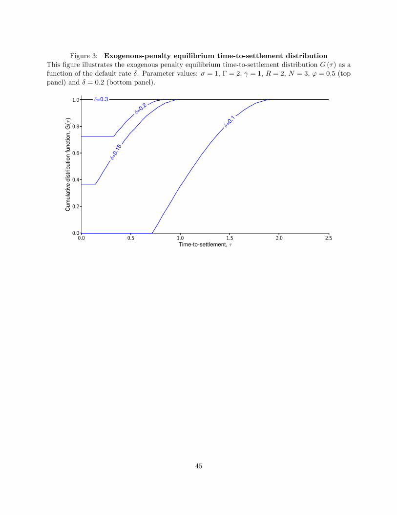
Figure 3: Exogenous-penalty equilibrium time-to-settlement distributionThis figure illustrates the exogenous penalty equilibrium time-to-settlement distribution G (τ) as afunction of the default rate δ. Parameter values: σ = 1, Γ = 2, γ = 1, R = 2, N = 3, ϕ = 0.5 (toppanel) and δ = 0.2 (bottom panel).

0.0 0.5 1.0 1.5 2.0 2.5Time-to-settlement, τ

0.0

0.2

0.4

0.6

0.8

1.0

Cum

ulat

ive

dist

ribut

ion

func

tion,

G( τ

)

δ=0.1

δ=0.

18δ=

0.2δ=0.3

45

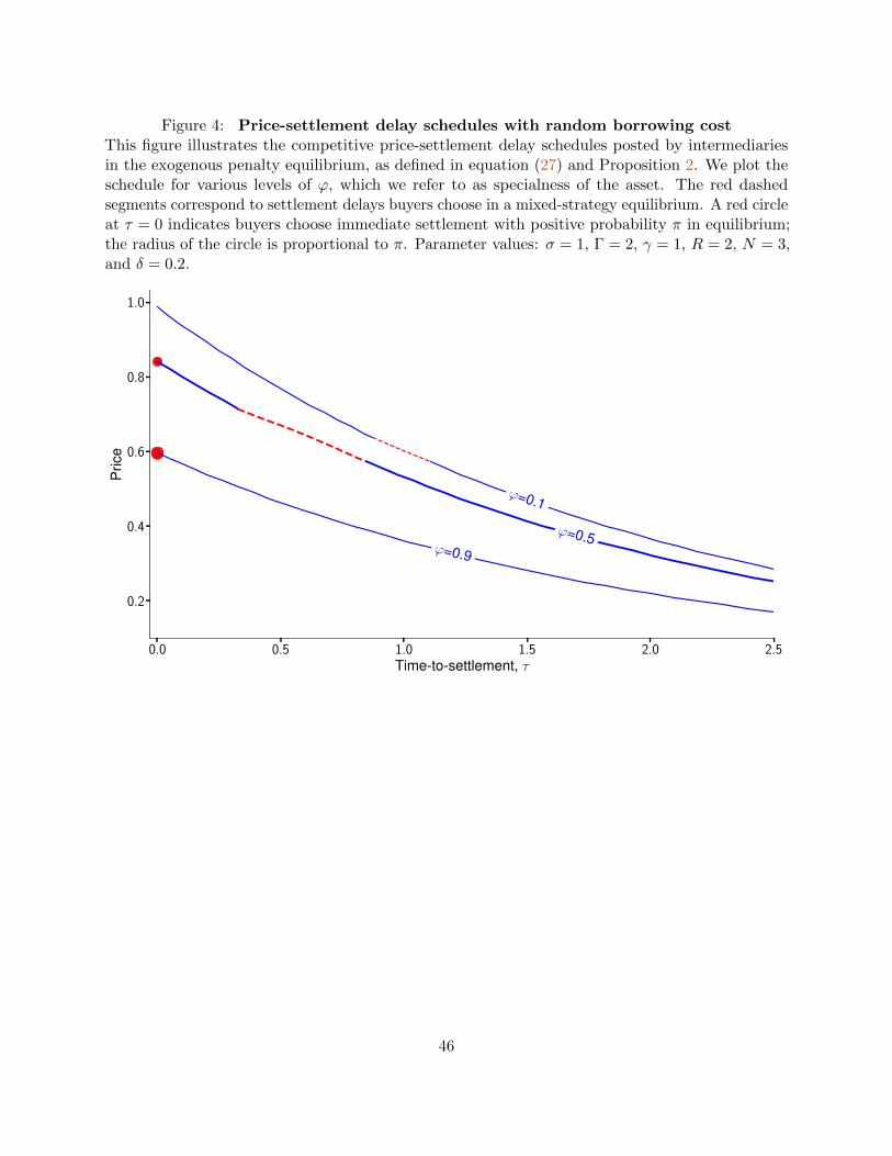
Figure 4: Price-settlement delay schedules with random borrowing costThis figure illustrates the competitive price-settlement delay schedules posted by intermediariesin the exogenous penalty equilibrium, as defined in equation (27) and Proposition 2. We plot theschedule for various levels of ϕ, which we refer to as specialness of the asset. The red dashedsegments correspond to settlement delays buyers choose in a mixed-strategy equilibrium. A red circleat τ = 0 indicates buyers choose immediate settlement with positive probability π in equilibrium;the radius of the circle is proportional to π. Parameter values: σ = 1, Γ = 2, γ = 1, R = 2, N = 3,and δ = 0.2.

0.0 0.5 1.0 1.5 2.0 2.5Time-to-settlement, τ

0.2

0.4

0.6

0.8

1.0

Pric

e

ϕ=0.1

ϕ=0.5ϕ=0.9

46

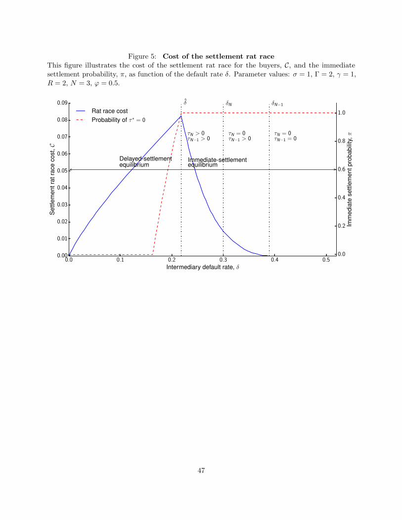
Figure 5: Cost of the settlement rat raceThis figure illustrates the cost of the settlement rat race for the buyers, C, and the immediatesettlement probability, π, as function of the default rate δ. Parameter values: σ = 1, Γ = 2, γ = 1,R = 2, N = 3, ϕ = 0.5.

0.0 0.1 0.2 0.3 0.4 0.5Intermediary default rate, δ

0.00

0.01

0.02

0.03

0.04

0.05

0.06

0.07

0.08

0.09

Set

tlem

entr

atra

ceco

st,C

0.0

0.2

0.4

0.6

0.8

1.0

Imm

edia

tese

ttlem

entp

roba

bilit

y,π

Immediate-settlementequilibrium

Delayed-settlementequilibrium

δN δN−1δ

τN > 0τN−1 > 0

τN = 0τN−1 > 0

τN = 0τN−1 = 0

Rat race costProbability of τ ? = 0

47

Figure 6: Failure-to-deliver penalty schedules if intermediary always borrowsThis figure illustrates the equilibrium failure-to-deliver penalty schedules posted by intermediaries,defined in equation (27) and Proposition 3. We plot the schedule for various levels of ϕ, which werefer to as specialness of the asset. Parameter values: θ = 2, σ = 1, Γ = 2, γ = 1, R = 2, N = 3,and δ = 0.2.

0.0 0.5 1.0 1.5 2.0 2.5Time-to-settlement, τ

0.0

0.1

0.2

0.3

0.4

Failu

re-to

-del

iver

pena

lty

ϕ=0.1

ϕ=0.5

ϕ=0.9

48

Figure 7: Failure-to-deliver probabilityThis figure illustrates the equilibrium failure-to-deliver probability for a B-I trade, as a functionof the asset specialness ϕ. We plot the schedule for various levels of intermediary default rates δ.Parameter values: θ = 2, σ = 1, Γ = 2, γ = 1, R = 2, N = 3, and δ = 0.2.

1.0 0.8 0.6 0.4 0.2 0.0Asset specialness (ϕ)

0.0

0.2

0.4

0.6

0.8

1.0

Failu

reto

deliv

erpr

obab

ility

δ=0.1

δ=0.5

δ=0.7

49

Figure 8: Expected rents of security lendersThis figure illustrates the expected utility of a security lender, conditional on owning the asset, as afunction of the intermediary default rate δ. We plot the schedule for various levels of ϕ, which werefer to as specialness of the asset. Parameter values: θ = 2, σ = 1, Γ = 2, γ = 1, R = 2, N = 3,and δ = 0.2.

0.0 0.1 0.2 0.3 0.4 0.5 0.6 0.7 0.8Intermediary default rate (δ)

0.00

0.02

0.04

0.06

0.08

0.10

0.12

0.14

Exc

ess

utili

tyfo

rase

curit

yle

nder

ϕ=0.3

ϕ=0.5

ϕ=0.7

δδ+λθ >

Γ2σ

2 (R − 1)δδ+λθ ≤

γ2σ

2 (R − 1)

50