Embed Size (px)
Citation preview
Smart Emission DocumentationRelease 1.0.0
Thijs Brentjens, Just van den Broecke, Michel Grothe
13 February 2019 at 03:09:05

Contents
1 Intro 3
2 Architecture 7
3 Components 17
4 Data Management 21
5 Calibration 43
6 Web Services 53
7 Dataflow and APIs 57
8 API and Code 61
9 Installation 63
10 Kubernetes 85
11 Sensors 93
12 Administration 97
13 Dissemination 109
14 Cookbook 115
15 Evolution 127
16 Contact 135
17 Links 137
18 Notes 139
19 Indices and tables 143
i

ii
Smart Emission Documentation, Release 1.0.0
Contents:
Contents 1
Smart Emission Documentation, Release 1.0.0
2 Contents

CHAPTER 1
Intro
This is the main (technical) documentation for the Smart Emission Data Platform. It can always be found at smart-platform.readthedocs.org. A somewhat lighter introduction can be found in this series of blogs.
The home page for the Smart Emission project and data platform is http://data.smartemission.nl
The home page for the Smart Emission Nijmegen project is http://smartemission.ruhosting.nl
The project GitHub repository is at https://github.com/smartemission/smartemission.
This is document version 1.0.0 generated on 12 February 2019 at 12:41:32.
1.1 History
The Smart Emission Platform was initiated and largely developed within the Smart Emission Nijmegen project (2015-2017, see also below).
The Geonovum/RIVM SOSPilot Project (2014-2015) , where RIVM LML (Dutch national Air Quality Data) datawas harvested and serviced via the OGC Sensor Observation Service (SOS), was a precursor for the architecture andapproach to ETL with sensor data.
In and after 2017 several other projects, web-clients and sensor-types started utilizing the platform hosted atdata.smartemission.nl. These include:
• the Smart City Living Lab: around 7 major cities within NL deployed Intemo sensor stations
• AirSensEUR - a EU JRC initiative for an Open Sensor HW/SW platform
This put more strain on the platform and required a more structural development and maintenance approach (thanproject-based funding).
In 2018, the SE Platform was migrated to the Dutch National GDI infrastructure PDOK maintained by the DutchKadaster. This gives a tremendous opportunity for long-term evolution and stability of the platform beyond the initialand project-based fundings. This migration targeted hosting within a Docker Kubernetes environment. All code wasmigrated to a dedicated Smart Emission GitHub Organization and hosting of all Docker Images on an SE DockerHubOrganization.
3

Smart Emission Documentation, Release 1.0.0
1.2 Smart Emission Nijmegen
The Smart Emission Platform was largely developed during the Smart Emission Nijmegen project started in 2015 andstill continuing.
Read all about the Smart Emission Nijmegen project via: smartemission.ruhosting.nl/.
An introductory presentation: http://www.ru.nl/publish/pages/774337/smartemission_ru_24juni_lc_v5_smallsize.pdf
In the paper Filling the feedback gap of place-related externalities in smart cities the project is described extensively.
“. . . we present the set-up of the pilot experiment in project “Smart Emission”, constructing an experimental citizen-sensor-network in the city of Nijmegen. This project, as part of research program ‘Maps 4 Society,’ is one of thecurrently running Smart City projects in the Netherlands. A number of social, technical and governmental innovationsare put together in this project: (1) innovative sensing method: new, low-cost sensors are being designed and builtin the project and tested in practice, using small sensing-modules that measure air quality indicators, amongst othersNO2, CO2, ozone, temperature and noise load. (2) big data: the measured data forms a refined data-flow from sensingpoints at places where people live and work: thus forming a ‘big picture’ to build a real-time, in-depth understandingof the local distribution of urban air quality (3) empowering citizens by making visible the ‘externality’ of urban airquality and feeding this into a bottom-up planning process: the community in the target area get the co-decision-making control over where the sensors are placed, co-interpret the mapped feedback data, discuss and collectivelyexplore possible options for improvement (supported by a Maptable instrument) to get a fair and ‘better’ distributionof air pollution in the city, balanced against other spatial qualities. . . . .”
The data from the Smart Emission sensors is converted and published as standard web services: OGC WMS(-Time),WFS, SOS and SensorThings APIs. Some web clients (SmartApp, Heron) are developed to visualize the data. All thisis part of the Smart Emission Data Platform whose technicalities are the subject of this document.
1.2.1 SE Nijmegen Project Partners
More on: http://smartemission.ruhosting.nl/over-ons/
1.3 Documentation Technology
Writing technical documentation using standalone documents like Word can be tedious especially for joint authoring,publication on the web and integration with code.
Luckily there are various open (web) technologies available for both document (joint) authoring and publication.
We use a combination of three technologies to automate documentation production, hence to produce this document:
1. Restructured Text (RST) as the document format
2. GitHub to allow joint authoring, versioning and safe storage of the raw (RST) document
3. ReadTheDocs.org (RTD) for document generation (on GH commits) and hosting on the web
This triple makes maintaining actualized documentation comfortable.
This document is written in Restructured Text (rst) generated by Sphinx and hosted by ReadTheDocs.org (RTD).
The sources of this document are (.rst) text files maintained in the Project’s GitHub: https://github.com/smartemission/smartemission/docs/platform
You can also download a PDF version of this document and even an Ebook version.
This document is automatically generated whenever a commit is performed on the above GitHub repository (via a“Post-Commit-Hook”)
4 Chapter 1. Intro

Smart Emission Documentation, Release 1.0.0
Fig. 1: Smart Emission Nijmegen Project Partners
1.3. Documentation Technology 5
Smart Emission Documentation, Release 1.0.0
Using Sphinx with RTD one effectively has a living document like a Wiki but with the structure and versioningcharacteristics of a real document or book.
Basically we let “The Cloud” (GitHub and RTD) work for us!
6 Chapter 1. Intro

CHAPTER 2
Architecture
This chapter describes the (software) architecture of the Smart Emission Data (Distribution) Platform. A recent pre-sentation (PDF) and this paper also may give more insight.
2.1 Global Architecture
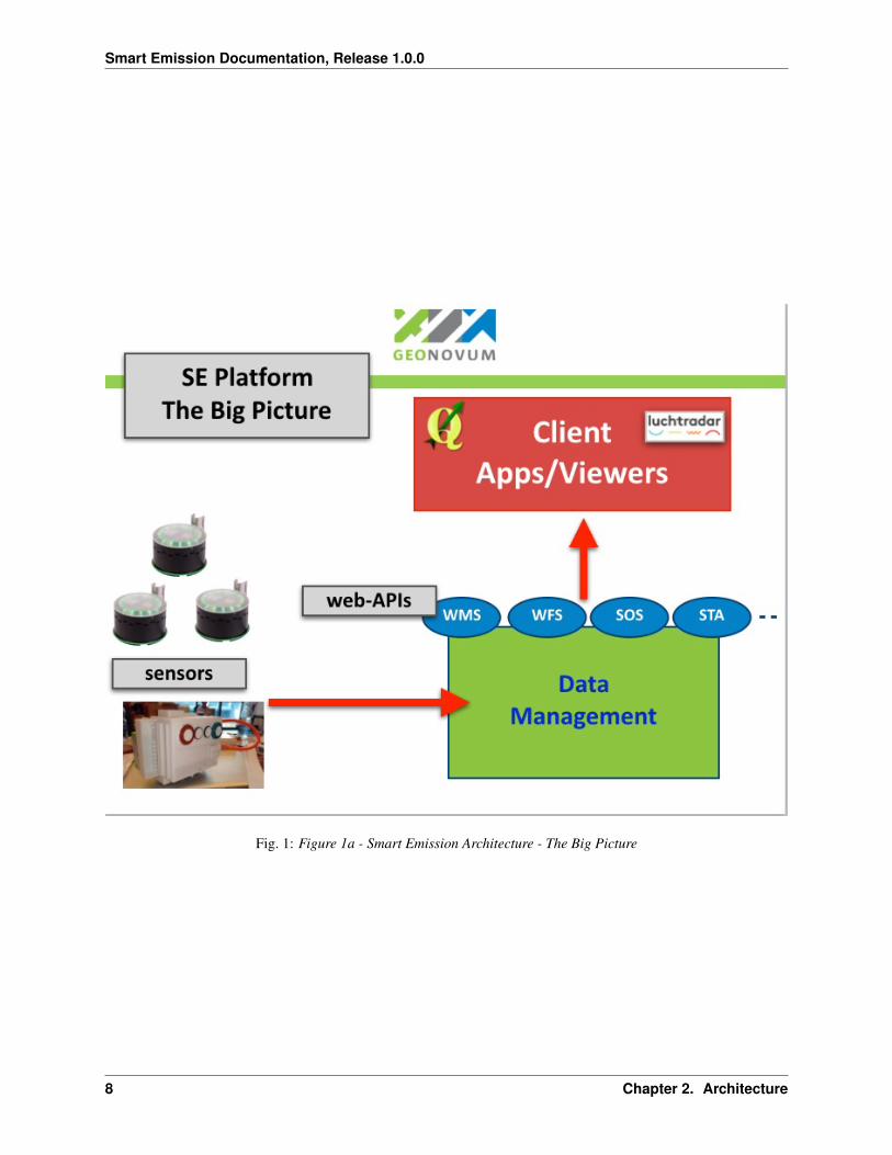
This section sketches “the big picture”: how the Smart Emission Data Platform fits into an overall/global architecturefrom sensor to citizen as depicted in Figure 1a and 1b below.
Figure 1a shows the main flow of data (red arrows) from sensors to viewers, in the following steps:
• Data is collected by sensors and sent to Data Management
• Data Management (ETL) is responsible for refining raw sensor data
• This refined (validated, calibrated, aggregated) sensor data is made available via Web Services
• Web Services include standardized OCG Web APIs like WMS (Time), WFS, SOS and the SensorThings API(STA)
• Viewers like the SmartApp and Heron and other clients use these Web APIs to fetch sensor (meta)data
Figure 1b expands on this architecture showing additional components and dataflows:
In Figure 1b the following is shown:
• Sensor stations (sensors) send (push) their raw data to Data Collectors
• A Data Collector functions as a buffer, keeping all data history using efficient bulk storage (InfluxDB, Mon-goDB, SOS)
• A Data Collector can be extern (blue) or internal (green) to the SE Data Platform
• A Data Collector provides an Web API through which its data (history) can be Harvested (pulled)
• The SE Data Platform continuously harvests all sensor data from Data Collectors (push/pull decoupling)
7
Smart Emission Documentation, Release 1.0.0
Fig. 1: Figure 1a - Smart Emission Architecture - The Big Picture
8 Chapter 2. Architecture

Smart Emission Documentation, Release 1.0.0
Fig. 2: Figure 1b - Smart Emission Architecture - Expanded with Dataflows
2.1. Global Architecture 9

Smart Emission Documentation, Release 1.0.0
• A set of ETL (Extract, Transform, Load) components refines/aggregates the raw sensor data, making it availablevia web service APIs
• SOS LML harvesting is used for acquiring reference data for Calibration only
Some details for the Intemo Josene: The sensor installation is connected to a power supply and to the Internet. Internetconnection is made by WIFI or telecommunication network (using a GSM chip). The data streams are sent encryptedto a Data Collector (see above). The encrypted data is decrypted by a dedicated “Jose Input Service” that also insertsthe data streams into a MongoDB or InfluxDB database using JSON. This database is the source production databasewhere all raw sensor data streams of the Jose Sensor installation are stored. A dedicated REST API – the Raw SensorAPI nicknamed the Whale API - is developed by CityGIS and Geonovum for further distribution of the SE data toother platforms.
In order to store the relevant SE data in the distribution database harvesting and pre-processing of the raw sensordata (from the CityGIS and Intemo Data Collectors) is performed. First, every N minutes a harvesting mechanismcollects sensor-data from the Data Collectors using the Raw Sensor API. The data encoded in JSON is then processedby a multi-step ETL-based pre-processing mechanism. In several steps the data streams are transformed to the Post-gres/PostGIS database. For instance, pre-processing is done specifically for the raw data from the air quality sensors.Based on a calibration activity in de SE project, the raw data from the air quality sensors is transformed to ‘betterinterpretable’ values. Post-processing is the activity to transform the pre-processed values into new types of data usingstatistics (aggregations), spatial interpolations, etc..
The design of the Smart Emission Data Platform, mainly the ETL design, is further expanded below.
2.2 Data Platform Architecture
Figure 2 below sketches the overall architecture with an emphasis on the flow of data (arrows). Circles depict harvest-ing/ETL processes. Server-instances are in rectangles. Datastores the “DB”-cons.
Fig. 3: Figure 2 - Smart Emission Data Platform ETL Context
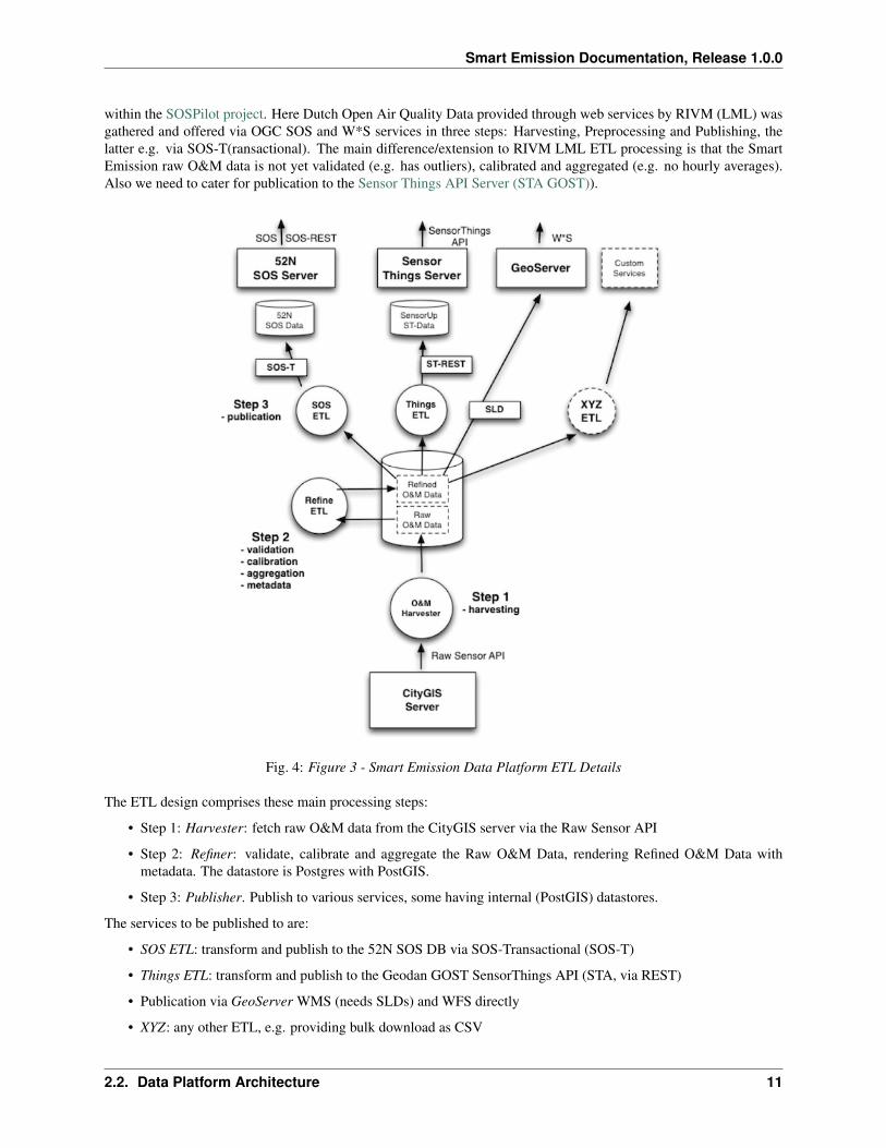
This global architecture is elaborated in more detail below. Figure 3 sketches a multistep-ETL approach as used
10 Chapter 2. Architecture
Smart Emission Documentation, Release 1.0.0
within the SOSPilot project. Here Dutch Open Air Quality Data provided through web services by RIVM (LML) wasgathered and offered via OGC SOS and W*S services in three steps: Harvesting, Preprocessing and Publishing, thelatter e.g. via SOS-T(ransactional). The main difference/extension to RIVM LML ETL processing is that the SmartEmission raw O&M data is not yet validated (e.g. has outliers), calibrated and aggregated (e.g. no hourly averages).Also we need to cater for publication to the Sensor Things API Server (STA GOST)).
Fig. 4: Figure 3 - Smart Emission Data Platform ETL Details
The ETL design comprises these main processing steps:
• Step 1: Harvester: fetch raw O&M data from the CityGIS server via the Raw Sensor API
• Step 2: Refiner: validate, calibrate and aggregate the Raw O&M Data, rendering Refined O&M Data withmetadata. The datastore is Postgres with PostGIS.
• Step 3: Publisher. Publish to various services, some having internal (PostGIS) datastores.
The services to be published to are:
• SOS ETL: transform and publish to the 52N SOS DB via SOS-Transactional (SOS-T)
• Things ETL: transform and publish to the Geodan GOST SensorThings API (STA, via REST)
• Publication via GeoServer WMS (needs SLDs) and WFS directly
• XYZ: any other ETL, e.g. providing bulk download as CSV
2.2. Data Platform Architecture 11
Smart Emission Documentation, Release 1.0.0
Some more notes for the above dataflows:
• The central DB will be Postgres with PostGIS enabled
• Refined O&M data can be directly used for OWS (WMS/WFS) services via GeoServer (using SLDs and aPostGIS datastore with selection VIEWs, e.g. last values of component X)
• The SOS ETL process transforms refined O&M data to SOS Observations and publishes these via the SOS-TInsertObservation service. Stations are published once via the InsertSensor service.
• Publication to the GOST SensorThings Server goes via the STA REST service
• These three ETL steps run continuously (via Linux cronjobs)
• Each ETL-process applies “progress-tracking” by maintaining persistent checkpoint data. Consequently a pro-cess always knows where to resume, even after its (cron)job has been stopped or canceled. All processes caneven be replayed from time zero.
2.3 Deployment
Docker is the main building block for the SE Data Platform deployment architecture.
Docker . . . allows you to package an application with all of its dependencies into a standardized unit for softwaredevelopment.. Read more on https://docs.docker.com.
The details of Docker are not discussed here, there are ample sources on the web. One of the best, if not the best,introductory books on Docker is The Docker Book.
The SE Platform can be completely deployed using either Docker Compose or using Docker Kubernetes (K8s, abbre-viated). The platform hosted via PDOK is using K8s.
2.3.1 Docker Strategy
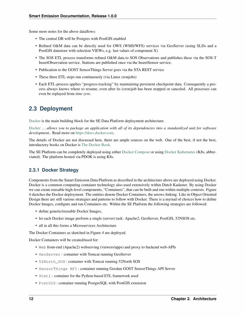
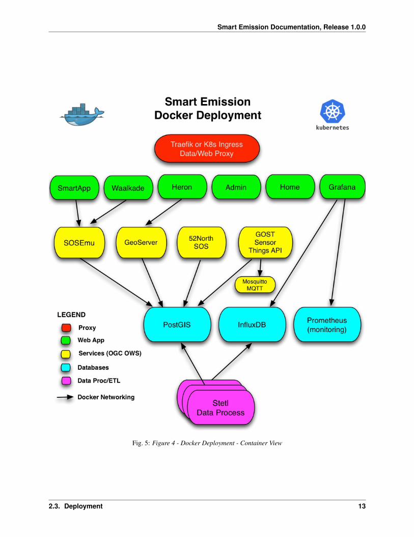
Components from the Smart Emission Data Platform as described in the architecture above are deployed using Docker.Docker is a common computing container technology also used extensively within Dutch Kadaster. By using Dockerwe can create reusable high-level components, “Containers”, that can be built and run within multiple contexts. Figure4 sketches the Docker deployment. The entities denote Docker Containers, the arrows linking. Like in Object OrientedDesign there are still various strategies and patterns to follow with Docker. There is a myriad of choices how to defineDocker Images, configure and run Containers etc. Within the SE Platform the following strategies are followed:
• define generic/reusable Docker Images,
• let each Docker image perform a single (server) task: Apache2, GeoServer, PostGIS, 52NSOS etc.
• all in all this forms a Microservices Architecture
The Docker Containers as sketched in Figure 4 are deployed.
Docker Containers will be created/used for:
• Web front-end (Apache2) webserving (viewers/apps) and proxy to backend web-APIs
• GeoServer : container with Tomcat running GeoServer
• 52North_SOS : container with Tomcat running 52North SOS
• SensorThings API : container running Geodan GOST SensorThings API Server
• Stetl : container for the Python-based ETL framework used
• PostGIS : container running PostgreSQL with PostGIS extension
12 Chapter 2. Architecture
Smart Emission Documentation, Release 1.0.0
Fig. 5: Figure 4 - Docker Deployment - Container View
2.3. Deployment 13

Smart Emission Documentation, Release 1.0.0
• InfluxDB: container running InfluxDB server from InfluxData
• Chronograf: container running Chronograf (InfluxDB Admin) from InfluxData
• Grafana: container running Grafana Dashboard
• MQTT: container running Mosquitto MQTT
The Docker Networking capabilities of Docker will be applied to link Docker Containers, for example to linkGeoServer and the other application servers to PostGIS. Docker Networking may be even applied (VM-) locationindependent, thus when required Containers may be distributed over VM-instances. Initially all data, logging, con-figuration and custom code/(web)content was maintained Local, i.e. on the host, outside Docker Containers/images.This will made the Docker Containers less reusable. Later, during PDOK migration, most Docker Images were madeself-contained as much as possible.
An Administrative Docker Component is also present. Code, content and configuration is maintained/synced in/withGitHub (see below). Docker Images are available publicly via Docker Hub.
The list of Docker-based components is available in the Components chapter.
See https://github.com/smartemission for the generic Docker images.
2.3.2 Test and Production
In order to provide a continuous/uninterrupted service both a Test and Production deployment has been setup. Forlocal development on PC/Mac/Linux a Vagrant environment with Docker can be setup.
The Test and Production environments have separate IP-adresses and domains: test.smartemission.nl anddata.smartemission.nl respectively.
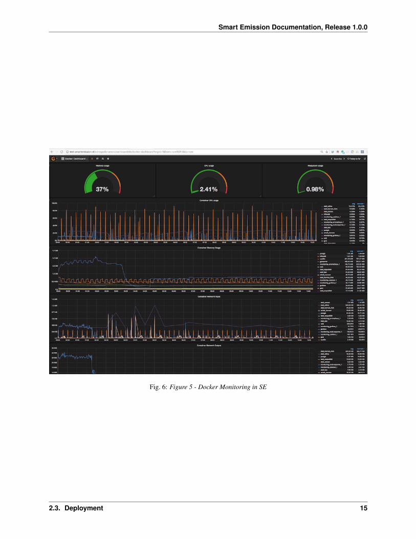
2.3.3 Monitoring
The challenge is to monitor services contained in Docker.
Monitoring is based around Prometheus and a dedicated (for monitoring) Grafana instance. A complete monitoringstack is deployed via docker-compose based on the Docker Monitoring Project. In the future this approach by StefanProdan is worthwhile.
14 Chapter 2. Architecture
Smart Emission Documentation, Release 1.0.0
Fig. 6: Figure 5 - Docker Monitoring in SE
2.3. Deployment 15

Smart Emission Documentation, Release 1.0.0
16 Chapter 2. Architecture

CHAPTER 3
Components
This chapter gives an overview of all components within the SE Platform and how they are organized into a(Docker/Kubernetes) microservices architecture.
A Component in this architecture is typically realized by a Docker Container as a configured instance of its DockerImage. A Component typically provides a (micro)Service and uses/depends on the services of other Components. Adeployed Component is as much self-contained as possible, for example a Component has no host-specific dependen-cies like Volume mappings etc.
Docker Images for SE Components are maintained in the SE GitHub Organization and made available via the SEDocker Hub
Components are also divided into (functional) categories, being:
• Apps - user-visible web applications
• Services - API services providing spatiotemporal data (WMS, WFS, STA etc)
• ETL - data handling, conversions and transformations, ETL=Extract Transform Load
• Datastore - databases
• Mon - monitoring and healthchecking of the SE Platform
• Admin - administrative tools, access resticted to admin users
Some Components may fit in multiple categories. For example a Grafana App to visualize monitoring data will be anApp and Monitoring category.
These components are deployed within Kubernetes (2018, Kadaster PDOK migration).
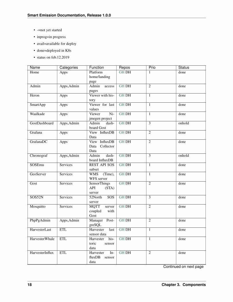
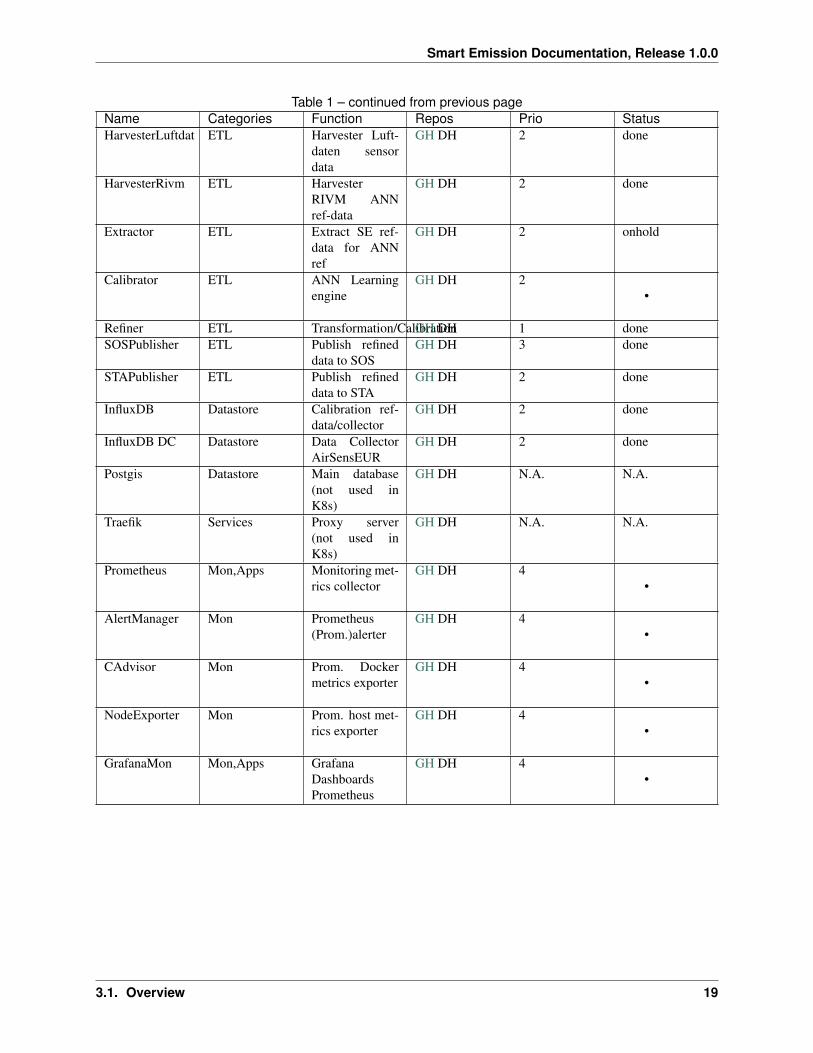
3.1 Overview
In the table below all Components are listed, their function, source (GitHub, GH) and Docker (Hub, DH) repositories,Categories, and for development strategy, their priority for the 2018 SE migration to Kubernetes (K8s). The “Status”column denotes the availability of the Docker Image for K8s deployment:
17
Smart Emission Documentation, Release 1.0.0
• -=not yet started
• inprog=in progress
• avail=available for deploy
• done=deployed in K8s
• status on feb.12.2019
Name Categories Function Repos Prio StatusHome Apps Platform
home/landingpage
GH DH 1 done
Admin Apps,Admin Admin accesspages
GH DH 2 done
Heron Apps Viewer with his-tory
GH DH 1 done
SmartApp Apps Viewer for lastvalues
GH DH 1 done
Waalkade Apps Viewer Ni-jmegen project
GH DH 1 done
GostDashboard Apps,Admin Admin dash-board Gost
GH DH 3 onhold
Grafana Apps View InfluxDBData
GH DH 2 done
GrafanaDC Apps View InfluxDBData CollectorData
GH DH 2 done
Chronograf Apps,Admin Admin dash-board InfluxDB
GH DH 3 onhold
SOSEmu Services REST API SOSsubset
GH DH 1 done
GeoServer Services WMS (Time),WFS server
GH DH 1 done
Gost Services SensorThingsAPI (STA)server
GH DH 2 done
SOS52N Services 52North SOSserver
GH DH 3 done
Mosquitto Services MQTT servercoupled withGost
GH DH 2 done
PhpPgAdmin Apps,Admin Manager Post-greSQL
GH DH 2 done
HarvesterLast ETL Harvester lastsensor data
GH DH 1 done
HarvesterWhale ETL Harvester his-toric sensordata
GH DH 1 done
HarvesterInflux ETL Harvester In-fluxDB sensordata
GH DH 2 done
Continued on next page
18 Chapter 3. Components
Smart Emission Documentation, Release 1.0.0
Table 1 – continued from previous pageName Categories Function Repos Prio StatusHarvesterLuftdat ETL Harvester Luft-
daten sensordata
GH DH 2 done
HarvesterRivm ETL HarvesterRIVM ANNref-data
GH DH 2 done
Extractor ETL Extract SE ref-data for ANNref
GH DH 2 onhold
Calibrator ETL ANN Learningengine
GH DH 2•
Refiner ETL Transformation/CalibrationGH DH 1 doneSOSPublisher ETL Publish refined
data to SOSGH DH 3 done
STAPublisher ETL Publish refineddata to STA
GH DH 2 done
InfluxDB Datastore Calibration ref-data/collector
GH DH 2 done
InfluxDB DC Datastore Data CollectorAirSensEUR
GH DH 2 done
Postgis Datastore Main database(not used inK8s)
GH DH N.A. N.A.
Traefik Services Proxy server(not used inK8s)
GH DH N.A. N.A.
Prometheus Mon,Apps Monitoring met-rics collector
GH DH 4•
AlertManager Mon Prometheus(Prom.)alerter
GH DH 4•
CAdvisor Mon Prom. Dockermetrics exporter
GH DH 4•
NodeExporter Mon Prom. host met-rics exporter
GH DH 4•
GrafanaMon Mon,Apps GrafanaDashboardsPrometheus
GH DH 4•
3.1. Overview 19
Smart Emission Documentation, Release 1.0.0
20 Chapter 3. Components
CHAPTER 4
Data Management
This chapter describes technical aspects of the data management, the ETL, of the Smart Emission (SE) Data Platform,expanding from the ETL-design in the Architecture chapter.
As sensor data is continuously generated, also ETL processing is a continuous multistep-sequence.
There are three main sequential ETL-steps:
• Harvesters - fetch raw sensor values from sensor data collectors like the “Whale server”
• Refiners - validate, convert, calibrate and aggregate raw sensor values
• Publishers - publish refined values to various (OGC) services
The Extractor is used for Calibration: it fetches reference and raw sensor data into an InfluxDB time-series DBas input for the Artificial Neural Network (ANN) learning process, called the Calibrator.
Implementation for all ETL can be found here: https://github.com/smartemission/docker-se-stetl.
4.1 General
This section describes general aspects applicable to all SE ETL processing.
4.1.1 Stetl Framework
The ETL-framework Stetl is used for all ETL-steps. The Stetl framework is an Open Source, general-purpose, ETLframework and programming model written in Python.
Each ETL-process is constructed by a Stetl config file. This config file specifies the Inputs, Filters and Outputs andparameters for that ETL-process. Stetl provides a multitude of reusable Inputs, Filters and Outputs. For example ready-to-use Outputs for Postgres and HTTP. For specific processing specific Inputs, Filters and Outputs can be developedby deriving from Stetl-base classes. This applies also to the SE-project.
For each ETL-step a specific Stetl config file is developed with some SE-specific Components.
SE Stetl processes are deployed and run using an SE Stetl Docker Image derived from the core Stetl Docker image.
21
Smart Emission Documentation, Release 1.0.0
4.1.2 ETL Scheduling
ETL processes run using the Unix cron scheduler or via K8s Job scheduler. See the SE Platform cronfile for theschedules.
4.1.3 Sync-tracking
Any continuous ETL, in particular in combination with data from remote systems, is liable to a multitude of failures:a remote server may be down, systems may be upgraded or restarted, the ETL software itself may be upgraded.Somehow an ETL-component needs to “keep track” of its last successful data processing: specifically for whichdevice, which sensor and which timestamp.
As programmatic tracking may suffer those same vulnerabilities, it was chosen to use the PostgreSQL (PG) databasefor tracking. Each of the three main ETL-steps will track its progress within PG-tables. In the cases of the Harvesterand the Refiner this synchronization is even strongly coupled to a PG TRIGGER: i.e. only if data has been successfullywritten/committed to the DB will the sync-state be updated. An ETL-process will always resume at the point of thelast saved sync-state.
4.1.4 Why Multistep?
Although all ETL could be performed within a single, continuous process, there are several reasons why a multistep,scheduled ETL processing from all Harvested data has been applied. “Multistep”, started by Harvesting (pull vs push)in combination with “sync-tracking” provides the following benefits:
• clear separation of concerns: Harvesting, Refining, Publishing
• all or individual ETL-steps can be “replayed” whenever some bug/enhancement appeared during development
• being more lean towards server downtime and network failures
• testing: each step can be thoroughly tested (using input data for that step)
• Harvesting (thus pull vs push) shields the SE Platform from “push overload”.
Each of the three ETL-steps are expanded below.
4.2 Harvesters
Harvesters fetch raw sensor data from remote raw sensor sources like data-collectors, services (e.g. SOS) ordatabases (e.g. InfluxDB). Currently there are Harvesters for CityGIS and Intemo data collectors for Josene devicesand InfluxDB databases for others like AirSensEUR devices. Harvesters are scheduled via cron. As a result a Harvesterwill store its raw data in the smartem_raw.timeseries database table (see below).
Harvesters, like all other ETL are developed using the Stetl ETL framework. As Stetl already supplies a Post-gres/PostGIS output, specific readers like the the Raw Sensor API needed to be developed: the RawSensorTime-seriesInput.
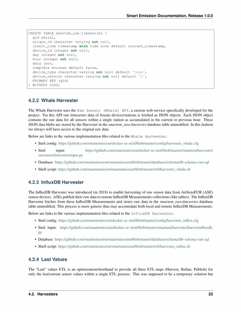
4.2.1 Database
The main table where Harvesters store data. Note the use of the data field as a json column. The device_id isthe unique station id.
22 Chapter 4. Data Management
Smart Emission Documentation, Release 1.0.0
CREATE TABLE smartem_raw.timeseries (gid serial,unique_id character varying not null,insert_time timestamp with time zone default current_timestamp,device_id integer not null,day integer not null,hour integer not null,data json,complete boolean default false,device_type character varying not null default 'jose',device_version character varying not null default '1',PRIMARY KEY (gid)
) WITHOUT OIDS;
4.2.2 Whale Harvester
The Whale Harvester uses the Raw Sensor (Whale) API, a custom web-service specifically developed for theproject. Via this API raw timeseries data of Josene devices/stations is fetched as JSON objects. Each JSON objectcontains the raw data for all sensors within a single station as accumulated in the current or previous hour. TheseJSON data blobs are stored by the Harvester in the smartem_raw.timeseries database table unmodified. In this fashionwe always will have access to the original raw data.
Below are links to the various implementation files related to the Whale Harvester.
• Stetl config: https://github.com/smartemission/docker-se-stetl/blob/master/config/harvester_whale.cfg
• Stetl input: https://github.com/smartemission/docker-se-stetl/blob/master/smartem/harvester/rawsensortimeseriesinput.py
• Database: https://github.com/smartemission/smartemission/blob/master/database/schema/db-schema-raw.sql
• Shell script: https://github.com/smartemission/smartemission/blob/master/etl/harvester_whale.sh
4.2.3 InfluxDB Harvester
The InfluxDB Harvester was introduced (in 2018) to enable harvesting of raw sensor data from AirSensEUR (ASE)sensor devices. ASEs publish their raw data to remote InfluxDB Measurements collections (like tables). The InfluxDBHarvester fetches from these InfluxDB Measurements and stores raw data in the smartem_raw.timeseries databasetable unmodified. This process is more generic thus may accomodate both local and remote InfluxDB Measurements.
Below are links to the various implementation files related to the InfluxDB Harvester.
• Stetl config: https://github.com/smartemission/docker-se-stetl/blob/master/config/harvester_influx.cfg
• Stetl input: https://github.com/smartemission/docker-se-stetl/blob/master/smartem/harvester/harvestinfluxdb.py
• Database: https://github.com/smartemission/smartemission/blob/master/database/schema/db-schema-raw.sql
• Shell script: https://github.com/smartemission/smartemission/blob/master/etl/harvester_influx.sh
4.2.4 Last Values
The “Last” values ETL is an optimization/shorthand to provide all three ETL-steps (Harvest, Refine, Publish) foronly the last/current sensor values within a single ETL process. This was supposed to be a temporary solution but
4.2. Harvesters 23
Smart Emission Documentation, Release 1.0.0
has survived and foun useful up to this day as the main drawback from the Harvester approach is the lack of real-time/pushed data.
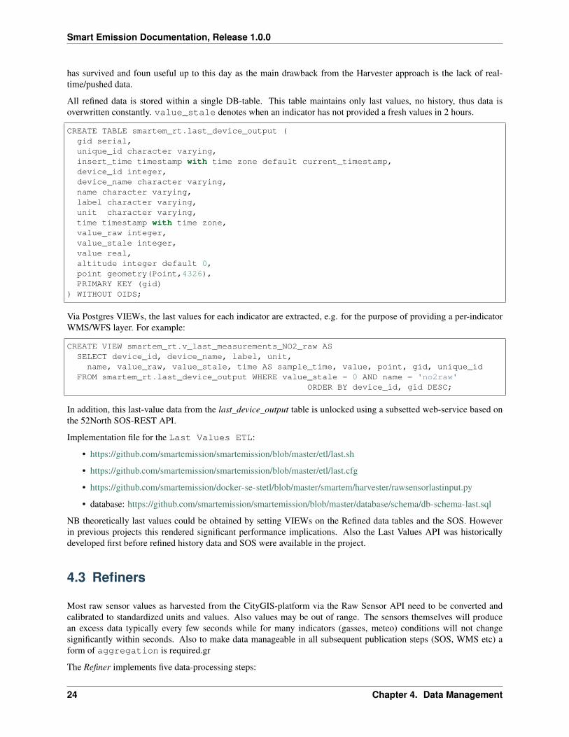
All refined data is stored within a single DB-table. This table maintains only last values, no history, thus data isoverwritten constantly. value_stale denotes when an indicator has not provided a fresh values in 2 hours.
CREATE TABLE smartem_rt.last_device_output (gid serial,unique_id character varying,insert_time timestamp with time zone default current_timestamp,device_id integer,device_name character varying,name character varying,label character varying,unit character varying,time timestamp with time zone,value_raw integer,value_stale integer,value real,altitude integer default 0,point geometry(Point,4326),PRIMARY KEY (gid)
) WITHOUT OIDS;
Via Postgres VIEWs, the last values for each indicator are extracted, e.g. for the purpose of providing a per-indicatorWMS/WFS layer. For example:
CREATE VIEW smartem_rt.v_last_measurements_NO2_raw ASSELECT device_id, device_name, label, unit,name, value_raw, value_stale, time AS sample_time, value, point, gid, unique_id
FROM smartem_rt.last_device_output WHERE value_stale = 0 AND name = 'no2raw'ORDER BY device_id, gid DESC;
In addition, this last-value data from the last_device_output table is unlocked using a subsetted web-service based onthe 52North SOS-REST API.
Implementation file for the Last Values ETL:
• https://github.com/smartemission/smartemission/blob/master/etl/last.sh
• https://github.com/smartemission/smartemission/blob/master/etl/last.cfg
• https://github.com/smartemission/docker-se-stetl/blob/master/smartem/harvester/rawsensorlastinput.py
• database: https://github.com/smartemission/smartemission/blob/master/database/schema/db-schema-last.sql
NB theoretically last values could be obtained by setting VIEWs on the Refined data tables and the SOS. Howeverin previous projects this rendered significant performance implications. Also the Last Values API was historicallydeveloped first before refined history data and SOS were available in the project.
4.3 Refiners
Most raw sensor values as harvested from the CityGIS-platform via the Raw Sensor API need to be converted andcalibrated to standardized units and values. Also values may be out of range. The sensors themselves will producean excess data typically every few seconds while for many indicators (gasses, meteo) conditions will not changesignificantly within seconds. Also to make data manageable in all subsequent publication steps (SOS, WMS etc) aform of aggregation is required.gr
The Refiner implements five data-processing steps:
24 Chapter 4. Data Management
Smart Emission Documentation, Release 1.0.0
• Validation (pre)
• Calibration
• Conversion
• Aggregation
• Validation (post)
The implementation of these steps is in most cases specific per sensor-type. This has been abstracted via the Pythonbase class Device with specific implementations per sensor station: Josene, AirSensEUR etc.
Validation deals with removing outliers, values outside specific intervals. Calibration and Conversion go hand-in-hand: in many cases, like Temperature, the sensor-values are already calibrated but provided in another unit likemilliKelvin. Here a straightforward conversion applies. In particularly raw gas-values may come as resistance (kOhm)or voltage values. In most cases there is no linear relationship between these raw values and standard gas concentrationunits like mg/m3 or ppm. In those cases Calibration needs to be applied. This has been elaborated first for Josenesensors.
4.3.1 Calibration (Josene Sensors)
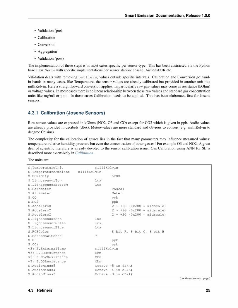
Raw sensor-values are expressed in kOhms (NO2, O3 and CO) except for CO2 which is given in ppb. Audio-valuesare already provided in decibels (dbA). Meteo-values are more standard and obvious to convert (e.g. milliKelvin todeegree Celsius).
The complexity for the calibration of gasses lies in the fact that many parameters may influence measured values:temperature, relative humidity, pressure but even the concentration of other gasses! For example O3 and NO2. A greatdeal of scientific literature is already devoted to the sensor calibration issue. Gas Calibration using ANN for SE isdescribed more extensively in Calibration.
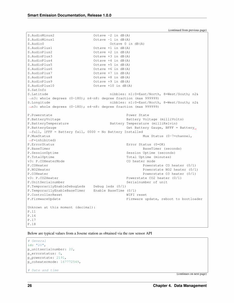
The units are:
S.TemperatureUnit milliKelvinS.TemperatureAmbient milliKelvinS.Humidity %mRHS.LightsensorTop LuxS.LightsensorBottom LuxS.Barometer PascalS.Altimeter MeterS.CO ppbS.NO2 ppbS.AcceleroX 2 ~ +2G (0x200 = midscale)S.AcceleroY 2 ~ +2G (0x200 = midscale)S.AcceleroZ 2 ~ +2G (0x200 = midscale)S.LightsensorRed LuxS.LightsensorGreen LuxS.LightsensorBlue LuxS.RGBColor 8 bit R, 8 bit G, 8 bit BS.BottomSwitches ?S.O3 ppbS.CO2 ppbv3: S.ExternalTemp milliKelvinv3: S.COResistance Ohmv3: S.No2Resistance Ohmv3: S.O3Resistance OhmS.AudioMinus5 Octave -5 in dB(A)S.AudioMinus4 Octave -4 in dB(A)S.AudioMinus3 Octave -3 in dB(A)
(continues on next page)
4.3. Refiners 25
Smart Emission Documentation, Release 1.0.0
(continued from previous page)
S.AudioMinus2 Octave -2 in dB(A)S.AudioMinus1 Octave -1 in dB(A)S.Audio0 Octave 0 in dB(A)S.AudioPlus1 Octave +1 in dB(A)S.AudioPlus2 Octave +2 in dB(A)S.AudioPlus3 Octave +3 in dB(A)S.AudioPlus4 Octave +4 in dB(A)S.AudioPlus5 Octave +5 in dB(A)S.AudioPlus6 Octave +6 in dB(A)S.AudioPlus7 Octave +7 in dB(A)S.AudioPlus8 Octave +8 in dB(A)S.AudioPlus9 Octave +9 in dB(A)S.AudioPlus10 Octave +10 in dB(A)S.SatInfoS.Latitude nibbles: n1:0=East/North, 8=West/South; n2&→˓n3: whole degrees (0-180); n4-n8: degree fraction (max 999999)S.Longitude nibbles: n1:0=East/North, 8=West/South; n2&→˓n3: whole degrees (0-180); n4-n8: degree fraction (max 999999)
P.Powerstate Power StateP.BatteryVoltage Battery Voltage (milliVolts)P.BatteryTemperature Battery Temperature (milliKelvin)P.BatteryGauge Get Battery Gauge, BFFF = Battery→˓full, 1FFF = Battery fail, 0000 = No Battery InstalledP.MuxStatus Mux Status (0-7=channel,→˓F=inhibited)P.ErrorStatus Error Status (0=OK)P.BaseTimer BaseTimer (seconds)P.SessionUptime Session Uptime (seconds)P.TotalUptime Total Uptime (minutes)v3: P.COHeaterMode CO heater modeP.COHeater Powerstate CO heater (0/1)P.NO2Heater Powerstate NO2 heater (0/1)P.O3Heater Powerstate O3 heater (0/1)v3: P.CO2Heater Powerstate CO2 heater (0/1)P.UnitSerialnumber Serialnumber of unitP.TemporarilyEnableDebugLeds Debug leds (0/1)P.TemporarilyEnableBaseTimer Enable BaseTime (0/1)P.ControllerReset WIFI resetP.FirmwareUpdate Firmware update, reboot to bootloader
Unknown at this moment (decimal):P.11P.16P.17P.18
Below are typical values from a Josene station as obtained via the raw sensor API
# Generalid: "20",p_unitserialnumber: 20,p_errorstatus: 0,p_powerstate: 2191,p_coheatermode: 167772549,
# Date and time(continues on next page)
26 Chapter 4. Data Management

Smart Emission Documentation, Release 1.0.0
(continued from previous page)
time: "2016-05-30T10:09:41.6655164Z",s_secondofday: 40245,s_rtcdate: 1069537,s_rtctime: 723501,p_totaluptime: 4409314,p_sessionuptime: 2914,p_basetimer: 6,
# GPSs_longitude: 6071111,s_latitude: 54307269,s_satinfo: 86795,
# Gas componementss_o3resistance: 30630,s_no2resistance: 160300,s_coresistance: 269275,
# Meteos_rain: 14,s_barometer: 100126,s_humidity: 75002,s_temperatureambient: 288837,s_temperatureunit: 297900,
# Audios_audioplus5: 1842974,v_audioplus4: 1578516,u_audioplus4: 1381393,t_audioplus4: 1907483,s_audioplus4: 1841174,v_audioplus3: 1710360,u_audioplus3: 1250066,t_audioplus3: 1842202,s_audioplus3: 1841946,v_audioplus2: 1381141,u_audioplus2: 1118225,t_audioplus2: 1645849,s_audioplus2: 1446679,v_audioplus1: 1381137,u_audioplus1: 1119505,t_audioplus1: 1776919,s_audioplus1: 1775382,v_audioplus9: 1710617,u_audioplus9: 1710617,t_audioplus9: 1841946,s_audioplus9: 1776409,v_audioplus8: 1512983,u_audioplus8: 1512982,t_audioplus8: 1578777,s_audioplus8: 1578776,v_audioplus7: 1381396,u_audioplus7: 1381396,t_audioplus7: 1512981,s_audioplus7: 1446932,v_audioplus6: 1249812,u_audioplus6: 1249555,
(continues on next page)
4.3. Refiners 27

Smart Emission Documentation, Release 1.0.0
(continued from previous page)
t_audioplus6: 2036501,s_audioplus6: 1315604,v_audioplus5: 1776923,u_audioplus5: 1710360,t_audioplus5: 2171681,v_audio0: 1184000,u_audio0: 986112,t_audio0: 1513984,s_audio0: 1249536,
# Lights_rgbcolor: 14546943,s_lightsensorblue: 13779,s_lightsensorgreen: 13352,s_lightsensorred: 11977,s_lightsensorbottom: 80,s_lightsensortop: 15981,
# Accelerometers_acceleroz: 783,s_acceleroy: 520,s_accelerox: 512,
# Unknownp_6: 1382167p_11: 40286,p_18: 167772549,p_17: 167772549,
Below each of these sensor values are elaborated. All conversions are implemented in using these Python scripts,called within the Stetl Refiner ETL process:
• josenedevice.py Device implementation
• josenedefs.py definitions of sensors
• josenefuncs.py mostly converter routines
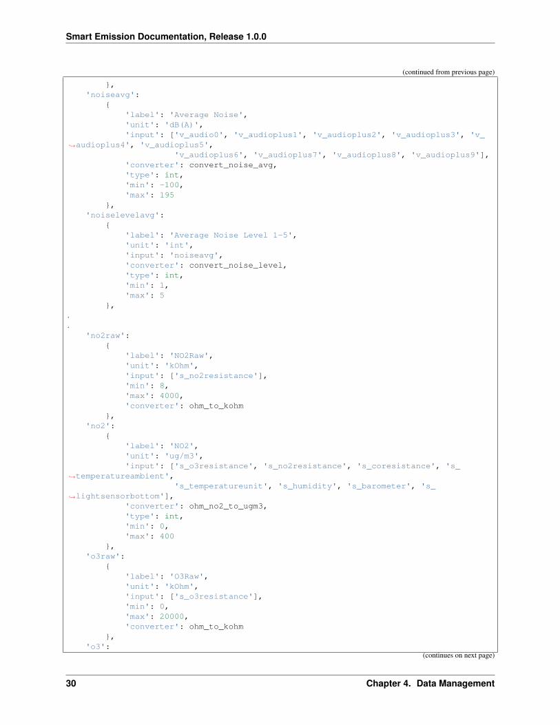
By using a generic config file josenedefs.py all validation and calibration is specified generically. Below some sampleentries.
SENSOR_DEFS = {..
# START Gasses Jose's_o3resistance':
{'label': 'O3Raw','unit': 'Ohm','min': 3000,'max': 6000000
},'s_no2resistance':
{'label': 'NO2RawOhm','unit': 'Ohm','min': 800,'max': 20000000
(continues on next page)
28 Chapter 4. Data Management

Smart Emission Documentation, Release 1.0.0
(continued from previous page)
},..
# START Meteo Jose's_temperatureambient':
{'label': 'Temperatuur','unit': 'milliKelvin','min': 233150,'max': 398150
},'s_barometer':
{'label': 'Luchtdruk','unit': 'HectoPascal','min': 20000,'max': 110000
},'s_humidity':
{'label': 'Relative Humidity','unit': 'm%RH','min': 20000,'max': 100000
},..
'temperature':{
'label': 'Temperatuur','unit': 'Celsius','input': 's_temperatureambient','converter': convert_temperature,'type': int,'min': -25,'max': 60
},'pressure':
{'label': 'Luchtdruk','unit': 'HectoPascal','input': 's_barometer','converter': convert_barometer,'type': int,'min': 200,'max': 1100
},'humidity':
{'label': 'Luchtvochtigheid','unit': 'Procent','input': 's_humidity','converter': convert_humidity,'type': int,'min': 20,'max': 100
(continues on next page)
4.3. Refiners 29
Smart Emission Documentation, Release 1.0.0
(continued from previous page)
},'noiseavg':
{'label': 'Average Noise','unit': 'dB(A)','input': ['v_audio0', 'v_audioplus1', 'v_audioplus2', 'v_audioplus3', 'v_
→˓audioplus4', 'v_audioplus5','v_audioplus6', 'v_audioplus7', 'v_audioplus8', 'v_audioplus9'],
'converter': convert_noise_avg,'type': int,'min': -100,'max': 195
},'noiselevelavg':
{'label': 'Average Noise Level 1-5','unit': 'int','input': 'noiseavg','converter': convert_noise_level,'type': int,'min': 1,'max': 5
},..
'no2raw':{
'label': 'NO2Raw','unit': 'kOhm','input': ['s_no2resistance'],'min': 8,'max': 4000,'converter': ohm_to_kohm
},'no2':
{'label': 'NO2','unit': 'ug/m3','input': ['s_o3resistance', 's_no2resistance', 's_coresistance', 's_
→˓temperatureambient','s_temperatureunit', 's_humidity', 's_barometer', 's_
→˓lightsensorbottom'],'converter': ohm_no2_to_ugm3,'type': int,'min': 0,'max': 400
},'o3raw':
{'label': 'O3Raw','unit': 'kOhm','input': ['s_o3resistance'],'min': 0,'max': 20000,'converter': ohm_to_kohm
},'o3':
(continues on next page)
30 Chapter 4. Data Management

Smart Emission Documentation, Release 1.0.0
(continued from previous page)
{'label': 'O3','unit': 'ug/m3','input': ['s_o3resistance', 's_no2resistance', 's_coresistance', 's_
→˓temperatureambient','s_temperatureunit', 's_humidity', 's_barometer', 's_
→˓lightsensorbottom'],'converter': ohm_o3_to_ugm3,'type': int,'min': 0,'max': 400
},..}
Each entry has:
• label: name for display
• unit: the unit of measurement (uom)
• input: optionally one or more input Entries required for conversion (josenefuncs.py). May cascade.
• converter: pointer to Python conversion function
• type: value type
• min/max: valid range (for validation)
Entries starting with s_ denote Jose raw sensor indicators. Others like no2 are “virtual” (SE) indicators, i.e. derivedeventually from s_ indicators.
In the Refiner ETL-config the desired indicators are specified, for example: temperature,humidity,pressure,noiseavg,noiselevelavg,co2,o3,co,no2,o3raw,coraw,no2raw. In this fashion theRefiner remains generic: driven by required indicators and their Entries.
4.3.2 Gas Calibration with ANN (Josene)
Within the SE project a separate activity is performed for gas-calibration based on Big Data Analysis statistical meth-ods. Values coming from SE sensors were compared to actual RIVM reference values. By matching predicted valueswith RIVM-values, a formula for each gas-component is established and refined. The initial approach was to use linearanalysis methods. However, further along in the project the use of Artificial Neural Networks (ANN) appeared to bethe most promising.
Gas Calibration using ANN for SE is described more extensively in Calibration.
Source code for ANN Gas Calibration learning process: https://github.com/smartemission/docker-se-stetl/tree/master/smartem/calibrator .
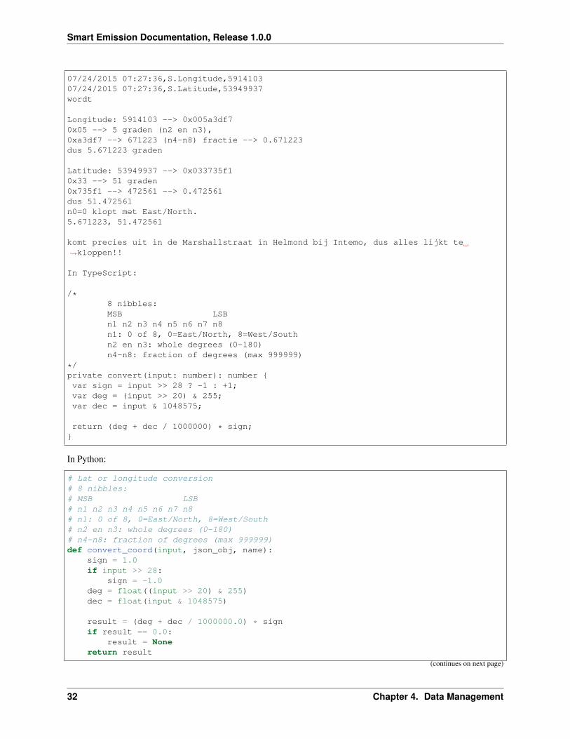
4.3.3 GPS Data (Josene)
GPS data from a Josene sensor is encoded in two integers: s_latitude and s_longitude. Below is the conversionalgoritm.
See https://github.com/Geonovum/sospilot/issues/22
Example:
4.3. Refiners 31
Smart Emission Documentation, Release 1.0.0
07/24/2015 07:27:36,S.Longitude,591410307/24/2015 07:27:36,S.Latitude,53949937wordt
Longitude: 5914103 --> 0x005a3df70x05 --> 5 graden (n2 en n3),0xa3df7 --> 671223 (n4-n8) fractie --> 0.671223dus 5.671223 graden
Latitude: 53949937 --> 0x033735f10x33 --> 51 graden0x735f1 --> 472561 --> 0.472561dus 51.472561n0=0 klopt met East/North.5.671223, 51.472561
komt precies uit in de Marshallstraat in Helmond bij Intemo, dus alles lijkt te→˓kloppen!!
In TypeScript:
/*8 nibbles:MSB LSBn1 n2 n3 n4 n5 n6 n7 n8n1: 0 of 8, 0=East/North, 8=West/Southn2 en n3: whole degrees (0-180)n4-n8: fraction of degrees (max 999999)
*/private convert(input: number): number {var sign = input >> 28 ? -1 : +1;var deg = (input >> 20) & 255;var dec = input & 1048575;
return (deg + dec / 1000000) * sign;}
In Python:
# Lat or longitude conversion# 8 nibbles:# MSB LSB# n1 n2 n3 n4 n5 n6 n7 n8# n1: 0 of 8, 0=East/North, 8=West/South# n2 en n3: whole degrees (0-180)# n4-n8: fraction of degrees (max 999999)def convert_coord(input, json_obj, name):
sign = 1.0if input >> 28:
sign = -1.0deg = float((input >> 20) & 255)dec = float(input & 1048575)
result = (deg + dec / 1000000.0) * signif result == 0.0:
result = Nonereturn result
(continues on next page)
32 Chapter 4. Data Management
Smart Emission Documentation, Release 1.0.0
(continued from previous page)
def convert_latitude(input, json_obj, name):res = convert_coord(input, json_obj, name)if res is not None and (res < -90.0 or res > 90.0):
log.error('Invalid latitude %d' % res)return None
return res
def convert_longitude(input, json_obj, name):res = convert_coord(input, json_obj, name)if res is not None and (res < -180.0 or res > 180.0):
log.error('Invalid longitude %d' % res)return None
return res
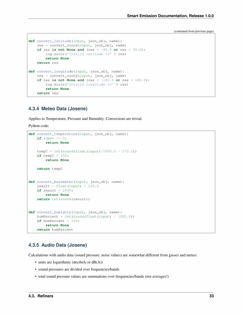
4.3.4 Meteo Data (Josene)
Applies to Temperature, Pressure and Humidity. Conversions are trivial.
Python code:
def convert_temperature(input, json_obj, name):if input == 0:
return None
tempC = int(round(float(input)/1000.0 - 273.1))if tempC > 100:
return None
return tempC
def convert_barometer(input, json_obj, name):result = float(input) / 100.0if result > 2000:
return Nonereturn int(round(result))
def convert_humidity(input, json_obj, name):humPercent = int(round(float(input) / 1000.0))if humPercent > 100:
return Nonereturn humPercent
4.3.5 Audio Data (Josene)
Calculations with audio data (sound pressure, noise values) are somewhat different from gasses and meteo:
• units are logarithmic (decibels or dB(A))
• sound pressures are divided over frequencies/bands
• total sound pressure values are summations over frequencies/bands (not averages!)
4.3. Refiners 33
Smart Emission Documentation, Release 1.0.0
These principles were not immediately understood and evolved during developement. See also some discussion aroundthis issue.
The links helped in understanding and check calculations via an online sound calculator:
• http://www.sengpielaudio.com/calculator-spl.htm
• http://www.sengpielaudio.com/calculator-octave.htm
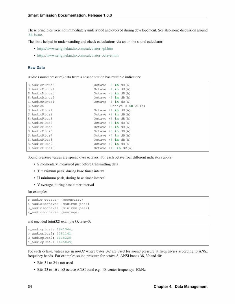
Raw Data
Audio (sound pressure) data from a Josene station has multiple indicators:
S.AudioMinus5 Octave -5 in dB(A)S.AudioMinus4 Octave -4 in dB(A)S.AudioMinus3 Octave -3 in dB(A)S.AudioMinus2 Octave -2 in dB(A)S.AudioMinus1 Octave -1 in dB(A)S.Audio0 Octave 0 in dB(A)S.AudioPlus1 Octave +1 in dB(A)S.AudioPlus2 Octave +2 in dB(A)S.AudioPlus3 Octave +3 in dB(A)S.AudioPlus4 Octave +4 in dB(A)S.AudioPlus5 Octave +5 in dB(A)S.AudioPlus6 Octave +6 in dB(A)S.AudioPlus7 Octave +7 in dB(A)S.AudioPlus8 Octave +8 in dB(A)S.AudioPlus9 Octave +9 in dB(A)S.AudioPlus10 Octave +10 in dB(A)
Sound pressure values are spread over octaves. For each octave four different indicators apply:
• S momentary, measured just before transmitting data
• T maximum peak, during base timer interval
• U minimum peak, during base timer interval
• V average, during base timer interval
for example:
s_audio<octave> (momentary)t_audio<octave> (maximum peak)u_audio<octave> (minimum peak)v_audio<octave> (average)
and encoded (uint32) example Octave+3:
s_audioplus3: 1841946,v_audioplus2: 1381141,u_audioplus2: 1118225,t_audioplus2: 1645849,
For each octave, values are in uint32 where bytes 0-2 are used for sound pressure at frequencies according to ANSIfrequency bands. For example: sound pressure for octave 8, ANSI bands 38, 39 and 40:
• Bits 31 to 24 : not used
• Bits 23 to 16 : 1/3 octave ANSI band e.g. 40, center frequency: 10kHz
34 Chapter 4. Data Management

Smart Emission Documentation, Release 1.0.0
• Bits 15 to 8 : 1/3 octave ANSI band e.g. 39, center frequency: 8kHz
• Bits 7 to 0 : 1/3 octave ANSI band e.g. 38, center frequency: 6.3kHz
This requires decoding bytes 0,1,2 from each uint32 value, in Python:
bands = [float(input_value & 255), float((input_value >> 8) & 255), float((input_→˓value >> 16) & 255)]
Via a bit shift and bitmask (2pow8-1 or 255), an array of 3 band-values (bytes 0-2) for each frequency is decoded.
Calculating Noise Indicators
In the first approach only the average (V) indicators are taken and converted/aggregated into hourly values throughthe Refiner. There are requirements to produce more indicators like 5 minute aggregations and peak indicators. Twoindicators are produced:
• noiseavg average hourly noise in dB(A)
• noiselevelavg average hourly noise level (value 1-5)
Conversions are implemented as follows. First the definition from josenedefs.py:
'noiseavg':{
'label': 'Average Noise','unit': 'dB(A)','input': ['v_audio0', 'v_audioplus1', 'v_audioplus2', 'v_audioplus3', 'v_
→˓audioplus4', 'v_audioplus5','v_audioplus6', 'v_audioplus7', 'v_audioplus8'],
'meta_id': 'au-V30_V3F','converter': convert_noise_avg,'type': int,'min': 0,'max': 195
},'noiselevelavg':
{'label': 'Average Noise Level 1-5','unit': 'int','input': 'noiseavg','meta_id': 'au-V30_V3F','converter': convert_noise_level,'type': int,'min': 1,'max': 5
},
The convert_noise_avg() function takes all a selection (31,5Hz to 8kHz) of v_audio* audio values (sum per octave)and calculates the sum over all octaves, from josenefuncs.py. Note that subbands 0 (40 Hz) of v_audio0 and subband2 (10KHz) of v_audioplus8 are removed.
# Converts audio var and populates sum NB all in dB(A) !# Logaritmisch optellen van de waarden per frequentieband voor het verkrijgen van de→˓totaalwaarde:## 10^(waarde/10)# En dat voor de waarden van alle frequenties en bij elkaar tellen.
(continues on next page)
4.3. Refiners 35

Smart Emission Documentation, Release 1.0.0
(continued from previous page)
# Daar de log van en x10## Normaal tellen wij op van 31,5 Hz tot 8 kHz. In totaal 9 oktaafanden.# 31,5 63 125 250 500 1000 2000 4000 en 8000 Hz## Of 27 1/3 oktaafbanden: 25, 31.5, 40, 50, 63, 80, enzdef convert_noise_avg(value, json_obj, sensor_def, device=None):
# For each audio observation:# decode into 3 bands (0,1,2)# determine sum of these bands (sound for octave)# determine overall sum of all octave bands
# Extract values for bands 0-2input_names = sensor_def['input']dbMin = sensor_def['min']dbMax = sensor_def['max']
# octave_values = []for input_name in input_names:
input_value = json_obj[input_name]
# decode dB(A) values into 3 bands (0,1,2) for this octavebands = [float(input_value & 255), float((input_value >> 8) & 255),
→˓float((input_value >> 16) & 255)]
if input_name is 'v_audio0':# Remove 40Hz subbanddel bands[0]
elif input_name is 'v_audioplus8':# Remove 10KHz subbanddel bands[2]
# determine sum of these 3 bandsband_sum = 0band_cnt = 0for i in range(0, len(bands)):
band_val = bands[i]
# skip outliersif band_val < dbMin or band_val > dbMax:
continue
band_cnt += 1
# convert band value Decibel(A) to Bel and then get "real" value (power→˓10)
band_sum += math.pow(10, band_val / 10)# print '%s : band[%d]=%f band_sum=%f' %(name, i, bands[i], band_sum)
if band_cnt == 0:return None
# Take sum of "real" values and convert back to Bel via log10 and Decibel via→˓*10
# band_sum = math.log10(band_sum / float(band_cnt)) * 10.0band_sum = math.log10(band_sum) * 10.0
(continues on next page)
36 Chapter 4. Data Management

Smart Emission Documentation, Release 1.0.0
(continued from previous page)
# print '%s : avg=%d' %(name, band_sum)
if band_sum < dbMin or band_sum > dbMax:return None
# octave_values.append(round(band_sum))
# Gather valuesif 'noiseavg' not in json_obj:
# Initialize sum value to first 1/3 octave band valuejson_obj['noiseavg'] = band_sumjson_obj['noiseavg_total'] = math.pow(10, band_sum / 10)json_obj['noiseavg_cnt'] = 1
else:# Add 1/3 octave band value to total and derive dB(A) valuejson_obj['noiseavg_cnt'] += 1json_obj['noiseavg_total'] += math.pow(10, band_sum / 10)#json_obj['noiseavg'] = int(# round(math.log10(json_obj['noiseavg_total'] / json_obj['noiseavg_cnt
→˓']) * 10.0))json_obj['noiseavg'] = int(
round(math.log10(json_obj['noiseavg_total']) * 10.0))
if json_obj['noiseavg'] < dbMin or json_obj['noiseavg'] > dbMax:return None
# Determine octave nr from var name# json_obj['v_audiolevel'] = calc_audio_level(json_obj['v_audioavg'])# print 'Unit %s - %s band_db=%f avg_db=%d level=%d' % (json_obj['p_
→˓unitserialnumber'], sensor_def, band_sum, json_obj['v_audioavg'], json_obj['v_→˓audiolevel'] )
return json_obj['noiseavg']
From this value the noiselevelavg indicator is calculated:
# From https://www.teachengineering.org/view_activity.php?url=collection/nyu_/→˓activities/nyu_noise/nyu_noise_activity1.xml# level dB(A)# 1 0-20 zero to quiet room# 2 20-40 up to average residence# 3 40-80 up to noisy class, alarm clock, police whistle# 4 80-90 truck with muffler# 5 90-up severe: pneumatic drill, artillery,## Peter vd Voorn:# Voor het categoriseren van de meetwaarden kunnen we het beste beginnen bij de 20→˓dB(A).# De hoogte waarde zal 95 dB(A) zijn. Bijvoorbeeld een vogel van heel dichtbij.# Je kunt dit nu gewoon lineair verdelen in 5 categorieen. Ieder 15 dB. Het betreft→˓buiten meetwaarden.# 20 fluister stil# 35 rustige woonwijk in een stad# 50 drukke woonwijk in een stad# 65 wonen op korte afstand van het spoor# 80 live optreden van een band aan het einde van het publieksdeel. Praten is→˓mogelijk.# 95 live optreden van een band midden op een plein. Praten is onmogelijk.
(continues on next page)
4.3. Refiners 37

Smart Emission Documentation, Release 1.0.0
(continued from previous page)
def calc_audio_level(db):levels = [20, 35, 50, 65, 80, 95]level_num = 1for i in range(0, len(levels)):
if db > levels[i]:level_num = i + 1
return level_num
The hourly average is calculated by averaging all values within the Refiner:
# M = M + (x-M)/n# Here M is the (cumulative moving) average, x is the new value in the# sequence, n is the count of values. Using floats as not to loose precision.def moving_average(self, moving_avg, x, n, unit):
if 'dB' in unit:# convert Decibel to Bel and then get "real" value (power 10)# print moving_avg, x, nx = math.pow(10, x / 10)moving_avg = math.pow(10, moving_avg / 10)moving_avg = self.moving_average(moving_avg, x, n, 'int')# Take average of "real" values and convert back to Bel via log10 and Decibel
→˓via *10return math.log10(moving_avg) * 10.0
# Standard moving avg.return float(moving_avg) + (float(x) - float(moving_avg)) / float(n)
So summarizing Sound Pressure hourly values are calculated in three steps:
• sum sound pressure dB(A) per octave by summing its 1/3 octave subbands
• sum sound pressure dB(A) for all octaves
• calculate hourly average from these last sums
4.4 Publishers
A Publisher ETL process reads “Refined” indicator data and publishes these to various web-services. Most specif-ically this entails publication to:
• OGC Sensor Observation Service (SOS)
• OGC Sensor Things API (STA)
For both SOS and STA the transactional/REST web-services are used.
Publishing to OGC WMS and WFS is not explicitly required: these services can directly use the PostGIS databasetables and VIEWs produced by the Refiner. For WMS, GeoServer WMS Dimension for the “time” column isused together with SLDs that show values, in order to provide historical data via WMS. WFS can be used for bulkdownload.
4.4.1 General
The ETL chain is setup using the smartemdb.RefinedDbInput class directly coupled to a Stetl Output class, specific forthe web-service published to.
38 Chapter 4. Data Management
Smart Emission Documentation, Release 1.0.0
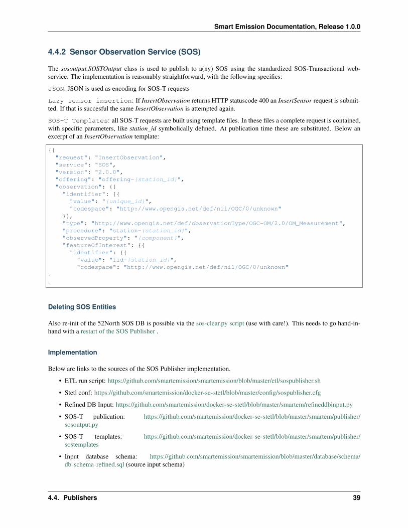
4.4.2 Sensor Observation Service (SOS)
The sosoutput.SOSTOutput class is used to publish to a(ny) SOS using the standardized SOS-Transactional web-service. The implementation is reasonably straightforward, with the following specifics:
JSON: JSON is used as encoding for SOS-T requests
Lazy sensor insertion: If InsertObservation returns HTTP statuscode 400 an InsertSensor request is submit-ted. If that is succesful the same InsertObservation is attempted again.
SOS-T Templates: all SOS-T requests are built using template files. In these files a complete request is contained,with specific parameters, like station_id symbolically defined. At publication time these are substituted. Below anexcerpt of an InsertObservation template:
{{"request": "InsertObservation","service": "SOS","version": "2.0.0","offering": "offering-{station_id}","observation": {{"identifier": {{
"value": "{unique_id}","codespace": "http://www.opengis.net/def/nil/OGC/0/unknown"
}},"type": "http://www.opengis.net/def/observationType/OGC-OM/2.0/OM_Measurement","procedure": "station-{station_id}","observedProperty": "{component}","featureOfInterest": {{
"identifier": {{"value": "fid-{station_id}","codespace": "http://www.opengis.net/def/nil/OGC/0/unknown"
.
.
Deleting SOS Entities
Also re-init of the 52North SOS DB is possible via the sos-clear.py script (use with care!). This needs to go hand-in-hand with a restart of the SOS Publisher .
Implementation
Below are links to the sources of the SOS Publisher implementation.
• ETL run script: https://github.com/smartemission/smartemission/blob/master/etl/sospublisher.sh
• Stetl conf: https://github.com/smartemission/docker-se-stetl/blob/master/config/sospublisher.cfg
• Refined DB Input: https://github.com/smartemission/docker-se-stetl/blob/master/smartem/refineddbinput.py
• SOS-T publication: https://github.com/smartemission/docker-se-stetl/blob/master/smartem/publisher/sosoutput.py
• SOS-T templates: https://github.com/smartemission/docker-se-stetl/blob/master/smartem/publisher/sostemplates
• Input database schema: https://github.com/smartemission/smartemission/blob/master/database/schema/db-schema-refined.sql (source input schema)
4.4. Publishers 39
Smart Emission Documentation, Release 1.0.0
• Re-init SOS DB schema (.sh): https://github.com/smartemission/smartemission/blob/master/services/sos52n/config/sos-clear.py
• Restart SOS Publisher (.sh): https://github.com/smartemission/smartemission/blob/master/database/util/sos-publisher-init.sh (inits last gis published to -1)
4.4.3 Sensor Things API (STA)
The STAOutput class is used to publish to any SensorThings API server using the standardized OGC SensorThingsREST API. The implementation is reasonably straightforward, with the following specifics:
JSON: JSON is used as encoding for STA requests.
Lazy Entity Insertion: At POST Observation it is determined via a REST GET requests if the cor-responding STA Entities, Thing, Location, DataStream etc are present. If not these are inserted via POSTrequests to the STA REST API and cached locally in the ETL process for the duration of the ETL Run.
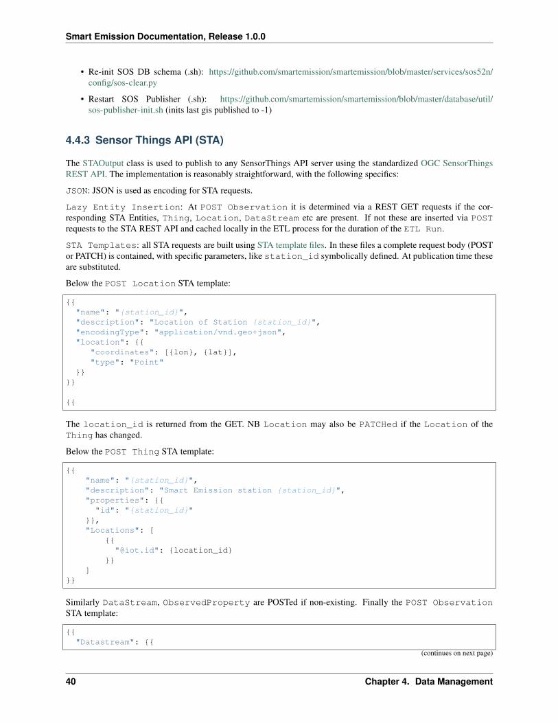
STA Templates: all STA requests are built using STA template files. In these files a complete request body (POSTor PATCH) is contained, with specific parameters, like station_id symbolically defined. At publication time theseare substituted.
Below the POST Location STA template:
{{"name": "{station_id}","description": "Location of Station {station_id}","encodingType": "application/vnd.geo+json","location": {{
"coordinates": [{lon}, {lat}],"type": "Point"
}}}}
{{
The location_id is returned from the GET. NB Location may also be PATCHed if the Location of theThing has changed.
Below the POST Thing STA template:
{{"name": "{station_id}","description": "Smart Emission station {station_id}","properties": {{
"id": "{station_id}"}},"Locations": [
{{"@iot.id": {location_id}
}}]
}}
Similarly DataStream, ObservedProperty are POSTed if non-existing. Finally the POST ObservationSTA template:
{{"Datastream": {{
(continues on next page)
40 Chapter 4. Data Management
Smart Emission Documentation, Release 1.0.0
(continued from previous page)
"@iot.id": {datastream_id}}},"phenomenonTime": "{sample_time}","result": {sample_value},"resultTime": "{sample_time}","parameters": {{
{parameters}}}
}}
4.4.4 Entity Mapping
Data records produced by the Refiner are mapped to STA Entities by the STA Publisher.
SE Artefact STA Entity ExampleStation Thing Intemo station AirSensEUR BoxStation point location Location AirSensEUR Box location at 4.982, 52.358 lon/latSensor Type/Metadata Sensor AlphaSense NO2B43FType and unit (uom) ObservedProperty NO2 in ug/m3Value and time Observation 42 ug/m3 on 1 aug 2018 13:42:45Combination of above Datastream Combines T, S, OP and OStation time+location HistoricalLocation AirSensEUR Box at lat/lon 52.35,4.92 on on 1 aug 2018 13:42:45Station Area FeatureOfInterest Location of Station 11820004
Deleting STA Entities
Also deletion of all Entities is possible via the staclear.py script (use with care!). This needs to go hand-in-hand witha restart of the STA Publisher .
Implementation
Below are links to the sources of the STA Publisher implementation.
• ETL run script: https://github.com/smartemission/smartemission/blob/master/etl/stapublisher.sh
• Stetl conf: https://github.com/smartemission/docker-se-stetl/blob/master/config/stapublisher.cfg
• Refined DB Input: https://github.com/smartemission/docker-se-stetl/blob/master/smartem/refineddbinput.py
• STA publication: https://github.com/smartemission/docker-se-stetl/blob/master/smartem/publisher/staoutput.py
• STA templates: https://github.com/smartemission/docker-se-stetl/blob/master/smartem/publisher/statemplates
• Input database schema: https://github.com/smartemission/smartemission/blob/master/database/schema/db-schema-refined.sql (source schema)
• Restart STA publisher (.sh): https://github.com/smartemission/smartemission/blob/master/database/util/sta-publisher-init.sh (inits last gis published to -1)
• Clear/init STA server (.sh): https://github.com/smartemission/smartemission/blob/master/database/util/staclear.sh (deletes all Entities!)
• Clear/init STA server (.py): https://github.com/smartemission/smartemission/blob/master/database/util/staclear.py (deletes all Entities!)
4.4. Publishers 41

Smart Emission Documentation, Release 1.0.0
42 Chapter 4. Data Management
CHAPTER 5
Calibration
This chapter describes how gas measurements in kOhm and ppb are translated to the standardized and ‘better inter-pretable’ units of ug/m3 (microgram per cubic meter).
The challenge is that Jose sensors produce noisy and biased measurements of gas components on a wrong scale. Thedata is noisy because two consecutive measurements of the same gas component can vary a lot. The measurementsare biased because the gas sensors are cross sensitive for (at least) temperature and other gas components. The mea-surements are on the wrong scale because the results in kOhm instead of the more interpretable ug/m3 or ppm. Theseissues are fixed by calibrating the Jose sensors to reliable RIVM measurements.
Data from Jose and RIVM is pre-processed before using it to train an Artificial Neural Network (ANN). The perfor-mance is optimized and the best model is chosen for online predictions.
These processes were initially executed manually. At a later stage, and thus currently, the entire ANN Calibrationprocess is automated.
The idea to use ANN emerged when initial calibration using Linear Regresssion-based methods did not render satis-factory results. From studying existing research like
• “Field calibration of a cluster of low-cost available sensors for air quality monitoring” by Spinelle, Gerboles etal
• “Air Temperature Estimation by Using Artificial Neural Network Models in the Greater Athens Area, Greece”by A. P. Kamoutsis et al.
ANN appeared a good candidate. Though complex when manually performed, we also aimed to overcome this byautomating both the learning and calibration process within the already existing SE ETL process pipelines.
5.1 Data
Data used for calibration (training the ANN) originates from Jose (raw data) and RIVM (reference data) stations thatare located pairwise in close proximity. They are located at the Graafseweg and Ruyterstraat in Nijmegen.
Data was gathered for a period of february 2016 to now.
Data was initially manually delivered:
43

Smart Emission Documentation, Release 1.0.0
• RIVM reference data by Jan Vonk (RIVM).
• Raw data from the Jose sensors by Robert Kieboom (CityGIS).
At a later stage, and thus currently, this data delivery is automated and continuous:
• RIVM data is harvested from the public RIVM LML SOS via the ETL Harvester_rivm
• Jose data is harvested from the Whale Server(s) via the ETL Harvester and then further extracted via the ETLExtractor
The overal datastream is depicted in Figure 1 below.
Fig. 1: Figure 1 - Overall setup ANN calibration
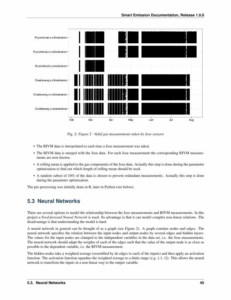
The harvested RIVM SOS data provides aggregated hour-records. Data from the Jose sensors have irregularities dueto lost wifi connection or power issues. Figure 2 below shows the periods of valid gas measurements taken by Josesensors.
5.2 Pre-processing
Before using the data form Jose and RIVM it needs to be pre-processed:
• Erroneous measurements are removed based on the error logs from RIVM and Jose.
• Extremely unlikely measurements are removed (e.g. gas concentrations below 0)
44 Chapter 5. Calibration
Smart Emission Documentation, Release 1.0.0
Fig. 2: Figure 2 - Valid gas measurements taken by Jose sensors
• The RIVM data is interpolated to each time a Jose measurement was taken.
• The RIVM data is merged with the Jose data. For each Jose measurement the corresponding RIVM measure-ments are now known.
• A rolling mean is applied to the gas components of the Jose data. Actually this step is done during the parameteroptimization to find out which length of rolling mean should be used.
• A random subset of 10% of the data is chosen to prevent redundant measurements. Actually this step is doneduring the parameter optimization.
The pre-processing was initially done in R, later in Python (see below).
5.3 Neural Networks
There are several options to model the relationship between the Jose measurements and RIVM measurements. In thisproject a Feed-forward Neural Network is used. Its advantage is that it can model complex non-linear relations. Thedisadvantage is that understanding the model is hard.
A neural network in general can be thought of as a graph (see Figure 2). A graph contains nodes and edges. Theneural network specifies the relation between the input nodes and output nodes by several edges and hidden layers.The values for the input nodes are clamped to the independent variables in the data set, i.e. the Jose measurements.The neural network should adapt the weights of each of the edges such that the value of the output node is as close aspossible to the dependent variable, i.e. the RIVM measurement.
The hidden nodes take a weighted average (resembled by de edges to each of the inputs) and then apply an activationfunction. The activation function squashes the weighted average to a finite range (e.g. [-1, 1]). This allows the neuralnetwork to transform the inputs in a non-linear way to the output variable.
5.3. Neural Networks 45

Smart Emission Documentation, Release 1.0.0
Fig. 3: Figure 3 - The structure of a Feed-forward Neural Network can be visualized as a graph
46 Chapter 5. Calibration
Smart Emission Documentation, Release 1.0.0
5.4 Training a Neural Network
A neural network is completely specified by the the weights between the nodes and the activation function of thenodes. The latter is specified on beforehand and thus only the weights should be learned during the training phase.
There is no way to find the optimal weights in an efficient way for an arbitrary neural network. Therefore, a lot ofmethods are proposed to iteratively approach the global optimum.
Most of them are based on the idea of back-propagation. With back-propagation the error for each of the records inthe data is used to change the weights slightly. The change in weights makes the error for that specific record lower.However, it might increase the error on other records. Therefore, only a tiny alteration is made for each error in eachrecord.
As an addition the used L-BFGS method also uses the first and second derivatives of the error function to convergefaster to a solution.
5.5 Performance evaluation
To evaluate the performance of the model the Root Mean Squared Error (RMSE) is used. The RMSE is the averageerror (prediction - actual value) of the model. Lower RMSE values are better.
Testing the model on the same data as it is trained on could lead to over-fitting. This means that the model learnrelations that are not there in practice. For this reason the performance evaluation needs to be done on different datathen the learning of the model. For example, 90% of the data is used to train the model and 10% is used to test themodel. This process can be repeated when using a different 10% to test the data. With the 90%-10% ratio this processcan be repeated 10 times. This is called cross validation. In practice, cross validation with 5 different splits of the datais used.
5.6 Parameter optimization
Training a neural network optimizes the weights between the nodes. However, the training process is also susceptibleto parameters. For example, the number of hidden nodes, the activation function of the hidden nodes, the learning rate,etc. can be set. For a complete list of all the parameters see the documentation of MLPRegressor.
Choosing different parameters for the neural network learning influences the performance and complexity of themodel. For example, using to few hidden nodes results in a model that cannot fit the pattern in the data. On the otherhand, using to many hidden nodes may model relationships that are to complex and do not generalize to unseen data.
Parameter optimization is the process of evaluating different parameters. RandomizedSearchCV from sklearn is usedto try different parameters and evaluate them using cross-validation. This method trains and evaluates a neural networkn_iter times. The actual code looks like this:
gs = RandomizedSearchCV(gs_pipe, grid, n_iter, measure_rmse, n_jobs=n_jobs,cv=cv_k, verbose=verbose, error_score=np.NaN)
gs.fit(x, y)
The first argument gs_pipe is the pipeline that filters the data and applies a neural network, grid is a collection withdistributions of possible parameters, n_iter is the number of parameters to try, measure_rmse is a function that com-putes the RMSE performance and cv_k specifies the number of cross-validations to run for each parameter setting.The other parameters control the process.
5.4. Training a Neural Network 47
Smart Emission Documentation, Release 1.0.0
5.7 Choosing the best model
A good model has a good performance but is also as simple as possible. Simpler models are less likely to over-fit, i.esimple models are less likely to fit relations that do not generalize to new data. For this reason, the simplest model thatperforms about as well (e.g. 1 standard deviation) as the best model is selected.
For each gas component this results in models with different learning parameters. Differences are in the size ofthe hidden layers, the learning rate, the regularization parameter, the momentum and the activation function . Formore information about these parameters check the documentation of MLPRegressor. The parameters for each gascomponent are listed below:
CO_final = {'mlp__hidden_layer_sizes': [56],'mlp__learning_rate_init': [0.000052997],'mlp__alpha': [0.0132466772],'mlp__momentum': [0.3377605568],'mlp__activation': ['relu'],'mlp__algorithm': ['l-bfgs'],'filter__alpha': [0.005]}
O3_final = {'mlp__hidden_layer_sizes': [42],'mlp__learning_rate_init': [0.220055322],'mlp__alpha': [0.2645091504],'mlp__momentum': [0.7904790613],'mlp__activation': ['logistic'],'mlp__algorithm': ['l-bfgs'],'filter__alpha': [0.005]}
NO2_final = {'mlp__hidden_layer_sizes': [79],'mlp__learning_rate_init': [0.0045013008],'mlp__alpha': [0.1382210543],'mlp__momentum': [0.473310471],'mlp__activation': ['tanh'],'mlp__algorithm': ['l-bfgs'],'filter__alpha': [0.005]}
5.8 Online predictions
The sensorconverters.py converter has routines to refine the Jose data. Here the raw Jose measurements for meteo andgas components are used to predict the hypothetical RIVM measurements of the gas components.
Three steps are taken to convert the raw Jose measurement to hypothetical RIVM measurements.
• The measurements are converted to the units with which the model is learned. For gas components this is kOhm,for temperature this is Celsius, humidity is in percent and pressure in hPa.
• A rolling mean removes extreme measurements. Currently the previous rolling mean has a weight of 0.995 andthe new value a weight of 0.005. Thus alpha is 0.005 in the following code:
def running_mean(previous_val, new_val, alpha):if new_val is None:
return previous_val
if previous_val is None:previous_val = new_val
val = new_val * alpha + previous_val * (1.0 - alpha)return val
48 Chapter 5. Calibration
Smart Emission Documentation, Release 1.0.0
• For each gas component a neural network model is used to predict the hypothetical RIVM measurements.Prediction are only made when all gas components are available. The actual prediction is made with this code:
# Predict RIVM value if all values are availableif None not in [o3, no2, co2, temp_amb, temp_unit, humidity, baro]:
value_array = np.array([baro, humidity, temp_amb, temp_unit, gasses['co2'],→˓gasses['no2'], gasses['o3']])
val = pipeline_objects[gas].predict(value_array.reshape(1, -1))[0]
return val
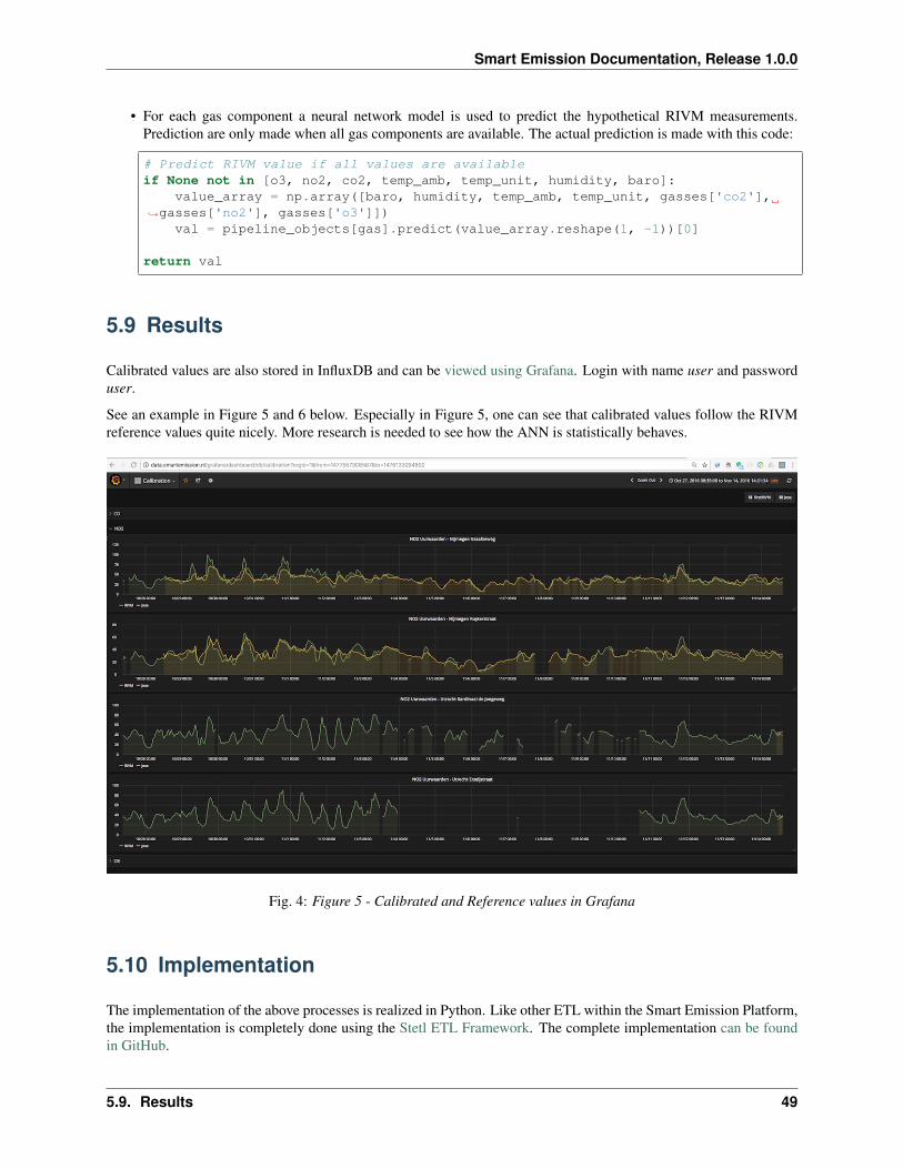
5.9 Results
Calibrated values are also stored in InfluxDB and can be viewed using Grafana. Login with name user and passworduser.
See an example in Figure 5 and 6 below. Especially in Figure 5, one can see that calibrated values follow the RIVMreference values quite nicely. More research is needed to see how the ANN is statistically behaves.
Fig. 4: Figure 5 - Calibrated and Reference values in Grafana
5.10 Implementation
The implementation of the above processes is realized in Python. Like other ETL within the Smart Emission Platform,the implementation is completely done using the Stetl ETL Framework. The complete implementation can be foundin GitHub.
5.9. Results 49
Smart Emission Documentation, Release 1.0.0
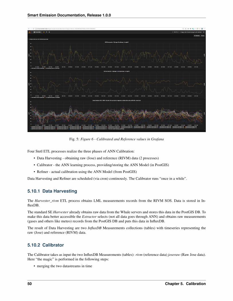
Fig. 5: Figure 6 - Calibrated and Reference values in Grafana
Four Stetl ETL processes realize the three phases of ANN Calibration:
• Data Harvesting - obtaining raw (Jose) and reference (RIVM) data (2 processes)
• Calibrator - the ANN learning process, providing/storing the ANN Model (in PostGIS)
• Refiner - actual calibration using the ANN Model (from PostGIS)
Data Harvesting and Refiner are scheduled (via cron) continously. The Calibrator runs “once in a while”.
5.10.1 Data Harvesting
The Harvester_rivm ETL process obtains LML measurements records from the RIVM SOS. Data is stored in In-fluxDB.
The standard SE Harvester already obtains raw data from the Whale servers and stores this data in the PostGIS DB. Tomake this data better accessible the Extractor selects (not all data goes through ANN) and obtains raw measurements(gases and others like meteo) records from the PostGIS DB and puts this data in InfluxDB.
The result of Data Harvesting are two InfluxDB Measurements collections (tables) with timeseries representing theraw (Jose) and reference (RIVM) data.
5.10.2 Calibrator
The Calibrator takes as input the two InfluxDB Measurements (tables): rivm (reference data) joseraw (Raw Jose data).Here “the magic” is performed in the following steps:
• merging the two datastreams in time
50 Chapter 5. Calibration
Smart Emission Documentation, Release 1.0.0
• performing the learning process
• storing the result ANN model in PostGIS
5.10.3 Refiner
This process takes raw data from the harvested timeseries data. By updating the sensordefs object with references tothe ANN model the raw data is calibrated via the sensorconverters and stored in PostGIS.
5.10. Implementation 51

Smart Emission Documentation, Release 1.0.0
52 Chapter 5. Calibration
CHAPTER 6
Web Services
This chapter describes how various mostly OGC OWS web services are realized on top of the converted/transformeddata as described in the data chapter. In particular:
• WFS and WMS-Time services
• OWS SOS (plus REST) service
• Smart Emission SOS Emulator service for Last Values
• SensorThings API
• InfluxDB + Chronograf
• Grafana
• Monitoring: Prometheus + Grafana
All services are defined under https://github.com/smartemission/smartemission/tree/master/services.
6.1 Web Frontend
All webservices, APIs and the website http://data.smartemission.nl are provided via an Apache2 HTTP server. Thisserver is the main outside entry to the platform and run via Docker.
Website and Viewers are run as a standard HTML website. The various API/OGC web-services are forwarded viaproxies to the backed-servers. For example GeoServer and the 52North SOS are connected via mod-proxy-ajp.
The SOS Emulator for Last Values is hosted as a Python Flask app.
6.1.1 Implementation
• Docker image: https://github.com/smartemission/smartemission/tree/master/docker/apache2
• Main dir: https://github.com/smartemission/smartemission/tree/master/services/web
• Running: https://github.com/smartemission/smartemission/tree/master/services/web/run.sh
53

Smart Emission Documentation, Release 1.0.0
• SOS Emulator: https://github.com/smartemission/smartemission/tree/master/services/api/sosrest
• Website and Viewers: https://github.com/smartemission/smartemission/tree/master/services/web/site
• Apache2 config: https://github.com/smartemission/smartemission/tree/master/services/web/config/sites-enabled
NB in 2018 this will be replaced by a setup using Traefik.
6.1.2 Links Traefik
• https://traefik.io/
• http://niels.nu/blog/2017/continuous-blog-delivery-p1.html
• https://www.digitalocean.com/community/tutorials/how-to-use-traefik-as-a-reverse-proxy-for-docker-containers-on-ubuntu-16-04
6.2 WFS and WMS Services
WMS and WFS are provided by GeoServer. These services are realized on top of the PostGIS tables/VIEWs resultingfrom the Refiner ETL process for timeseries (history) based layers and the “Last” table/VIEWs for Layers showingcurrent values.
The OGC standard WMS-Dimension facility is used to provide WMS layers for timeseries (history).
6.3 SOS Services
“The OGC Sensor Observation Service aggregates readings from live, in-situ and remote sensors. The service providesan interface to make sensors and sensor data archives accessible via an interoperable web based interface.”
The chapter on server administration describes how the SOS is deployed. This is called here the ‘SOS Server’.
The SOS server is provided using the 52North SOS web application (v4.3.7).
6.3.1 Docker for 52North SOS
Deployment of this SOS via Docker required some specific Docker features in order to deal with the 52North SOSconfiguration files.
During Docker build some specific configuration files are copied permanently into the Docker image as it is notpossible to map these via symlinks from host. These files are maintained in GitHub https://github.com/smartemission/smartemission/tree/master/docker/sos52n/resources/config:
• datasource.properties
• logback.xml
• timeseries-api_v1_beans.xml (just for Service Identification)
The third config file that the SOS needs is WEB-INF/configuration.db. In the Docker image this file is a symlink of/opt/sosconfig/configuration.db. A default version is provided. However, to be able to maintain this file over reruns ofthe Docker image a Docker volume mount should be done within the service invokation. This is done lazily within theDocker run file for the 52North SOS: https://github.com/smartemission/smartemission/blob/master/services/sos52n/run.sh On the first run the /opt/sosconfig is mapped locally (plus the SOS log dir). From then on configuration.db ismaintained on the host.
54 Chapter 6. Web Services
Smart Emission Documentation, Release 1.0.0
At runtime the sos52n Docker instance is linked to the postgis Docker instance.
6.3.2 Implementation
• Docker image: https://github.com/smartemission/smartemission/tree/master/docker/sos52n
• Running: https://github.com/smartemission/smartemission/tree/master/services/sos52n
6.4 SensorThings API
From https://wiki.tum.de/display/sddi/SensorThings+API :
“The OGC SensorThings API provides an open, geospatial-enabled and unified way to interconnect theInternet of Things (IoT) devices, data, and applications over the Web. The OGC SensorThings APIis an open standard, and that means it is non-proprietary, platform-independent, and perpetual royalty-free. Although it is a new standard, it builds on a rich set of proven-working and widely-adopted openstandards, such as the Web protocols and the OGC Sensor Web Enablement (SWE) standards, includingthe ISO/OGC Observation and Measurement (O&M) data model.
The main difference between the SensorThings API and the OGC Sensor Observation Service (SOS) isthat the SensorThings API is designed specifically for the resource-constrained IoT devices and the Webdeveloper community. As a result, the SensorThings API is lightweight and follows the REST principles,the use of an efficient JSON encoding, the use of MQTT protocol, the use of the flexible OASIS ODataprotocol and URL conventions.”
For the SensorThings API the Geodan GOST STA implementation is used.
The GOST server is available at http://data.smartemission.nl/gost/v1.0. The GOST Dashboard is available at http://data.smartemission.nl/adm/gostdashboard/ (admin access only).
NB all modifying HTTP methods (POST, PUT, DELETE, PATCH) and the GOST Dashboard are password-protected.
6.4.1 Implementation
Using two Docker Images: one for the GOST Server and one for the GOST Dashboard. The database is served fromthe SE PostGIS Docker Container.
• Docker image GOST Server: https://hub.docker.com/r/geodan/gost/
• Docker image GOST Dashboard v2: https://hub.docker.com/r/geodan/gost-dashboard-v2/
• Running: https://github.com/smartemission/smartemission/tree/master/services/gost
• Running: https://github.com/smartemission/smartemission/tree/master/services/gostdashboard
NB The Dashboard is not yet fully running via the SE web proxy pending this issue.
6.5 MQTT - Mosquitto
For the SensorThings API (GOST) MQTT is used. MQTT is a generic IoT protocol that can be used in other contextsbesides STA. NB MQTT is not currently in use within SE.
The MQTT server is available at http://data.smartemission.nl:1883 and http://data.smartemission.nl:9001
See also the GOST Dashboard at http://data.smartemission.nl/adm/gostdashboard/ (admin only).
6.4. SensorThings API 55

Smart Emission Documentation, Release 1.0.0
6.5.1 Implementation
• Docker image: https://hub.docker.com/r/toke/mosquitto/
• Running: https://github.com/smartemission/smartemission/tree/master/services/mosquitto
6.6 InfluxDB
InfluxDB has been added later in the project to support the Calibration process. For now this service is used internallyto collect both raw Sensor data and calibrated RIVM data.
At a later stage InfluxDB may get a more central role in the platform.
6.6.1 Implementation
• Docker image: https://hub.docker.com/_/influxdb/
• Running: https://github.com/smartemission/smartemission/tree/master/services/influxdb
6.7 Grafana
Grafana has been added later in the project to support InfluxDB visualization.
At a later stage Grafana may get a more central role in the platform.
6.7.1 Implementation
• Docker image: https://github.com/grafana/grafana-docker
• Running: https://github.com/smartemission/smartemission/tree/master/services/grafana
56 Chapter 6. Web Services
CHAPTER 7
Dataflow and APIs
This chapter focuses on dataflow and (external) protocol access to the SE Platform via so called Application Program-ming Interfaces (APIs).
See the Architecture and Data Management chapters for the overall design and data processing of the SE Platform.
7.1 Overview
This section sketches the global dataflow and introduces the main APIs.
Figure 1 above emphasizes the datastreams (red arrows) through the SE platform.
Data eventually always originates from sensors, mostly within stations like Intemo Josene or EU JRC AirSensEUR.Sensors are shown at the bottom of figure 1. One of the first observations is that sensors do not send their data directlyto the SE Platform, but push measurements to so called Data Collectors (drawn as squares). The SE Platform followsa pull model: data is continuously fetched from Data Collectors using Harvesters.
Further following the flow of data, the ETL processes (as described in Data Management) will eventually push therefined (validated, optionally aggregated, converted and/or calibrated) data to various API services that provide (mostlystandard OGC) Web APIs from which clients (e.g. Web Viewer Apps), even in theory another SE Harvester, canconsume the data.
There are two groups of APIs: Inbound (producer) APIs (in orange) and Outbound (consumer) APIs (in blue). In somecases the reason for an API-existence is historic: in the initial phase of the project, experience needed to be gainedwith multiple APIs. A short overview follows.
7.1.1 Inbound APIs
These are the APIs through which Harvesters pull (mainly raw) data into the platform.
57
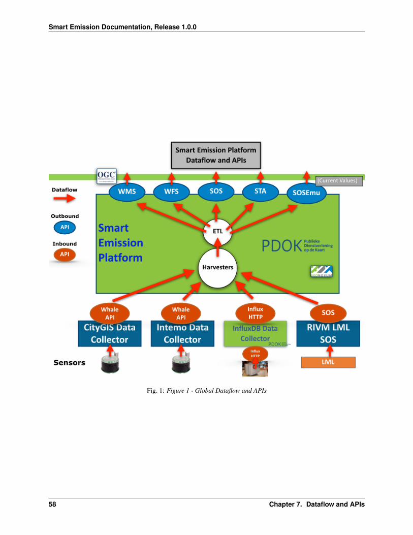
Smart Emission Documentation, Release 1.0.0
Fig. 1: Figure 1 - Global Dataflow and APIs
58 Chapter 7. Dataflow and APIs
Smart Emission Documentation, Release 1.0.0
Whale API a.k.a. Raw Sensor API
Via this API the SE Harvesters pull in data from Data Collectors. This custom Web API was developed (by RobertKieboom and Just van den Broecke) specifically for the project. As CityGIS already had developed a data collectionserver, but without data refinement and OGC services, a way was needed to transfer data to the SE Platform. APull/Harvesting model and API was chosen as it had advantages over a push-model:
• the SE Platform can pull-in data at its own pace
• resilient from restarts
• easier to deploy in an OTAP environment: e.g. both Test and Production servers can use the same Data Collectors
The specification and examples can be found in GitHub: https://github.com/smartemission/smartemission/tree/master/docs/specs/rawsensor-api.
The Whale API has two main services:
• fetch timeseries (history) data
• fetch latest data of any device
Devices in this case are Josene Sensors that contain multiple sensors, which together provide over 40 indicators. Themain classes are: gasses (for AQ), meteo (temperature etc), sound pressure (noise), GPS and misc data like lightintensity.
InfluxDB
Mainly used for AirSensEUR (ASE). Each ASE (mostly hourly) pushes its data to a remote InfluxDB. Per ASE stationa single InfluxDB Measurement (equivalent of a regular DB Table) is used.
Just like the Whale API, InfluxDB also provides an HTTP API to query Measurements and thus pull (harvest) time-series data.
An InfluxDB instance can be remote or within the same server as the rest of the SE Platform. This also provides ameans to couple a push-based model to a pull-based model.
Sensor Observation Service (SOS)
Data can be pulled from a remote SOS. For the SE platform this is used to pull in reference data from RIVM for theANN Calibration learning process. See also the Calibration chapter.
7.1.2 Outbound APIs
These are the APIs from which clients pull (mainly refined/aggregated) data from the platform.
Web Map Service (WMS)
A WMS with plain image and time-dimension support is provided. This allows clients to fetch images through history(e.g. with a timeslider in a web-viewer). The WMS OGC Standard provide Dimension-support, in this case time asdimension.
Endpoint: http://data.smartemission.nl/geoserver/wms?service=WMS&request=GetCapabilities
7.1. Overview 59
Smart Emission Documentation, Release 1.0.0
Web Feature Service (WFS)
This allows downloading of timeseries data with geospatial filter-support.
Endpoint: http://data.smartemission.nl/geoserver/wfs?service=WFS&request=GetCapabilities
Sensor Observation Service (SOS)
This provides a standard OGC SOS service: both the standard OGC versions 1 and 2, but also the 52North-specificSOS REST service.
Endpoint: http://data.smartemission.nl/sos52n/service?service=SOS&request=GetCapabilities
SensorThings API (STA)
This provides the SensorThings API, with requirements as SOS, but implemented much more lightweight. In a nut-shell: within STA an E/R-ike model of Entities (Things, Sensors, Datastreams, Observations etc) are managed viaHTTP verbs (like GET, PUT, PATCH etc).
NB the OGC STA standard also uses and integrates the IoT protocol MQTT. MQTT may be used in future SE Platformversions.
Endpoint: http://data.smartemission.nl/gost/v1.0
SOSEmu API
SOSEmu (SOS Emulator) has been developed early in the SE project, when SOS was not yet available, and a way wasneeded to quickly gain access to (Josene) sensor data. This API provides quick access to the latest (refined) data (nohistory support of Josene devices and has no support for other sensor device types) of sensors.
The main/only user is the SmartApp. SOSEmu is intended to be phased out.
Endpoint: http://data.smartemission.nl/sosemu
60 Chapter 7. Dataflow and APIs
CHAPTER 8
API and Code
Below is the API documention for the SE Platform Python code.
8.1 ETL Processes
Python classes involved in ETL. Code and config for all ETL can be found in the SE GitHub. All Python ETL code isunder the SE smartem Python Package.
61

Smart Emission Documentation, Release 1.0.0
62 Chapter 8. API and Code
CHAPTER 9
Installation
This chapter describes the installation steps for the Smart Emission Data Platform in a regular Docker environment.Note that installation and maintenance on Kubernetes is described in the :ref:‘kubernetes‘_ (K8s) chapter.
Currently http://test.smartemission.nl runs in this regular Docker environment, while the SE production http://data.smartemission.nl runs on K8s.
9.1 Principles
These are requirements and principles to understand and install an instance of the SE platform. It is required to havean understanding of Docker, as that is the main environment in which the SE Platform is run.
• Required OS: Ubuntu Linux 14.04 or later (tested on 14.04 and 16.04)
• all components are Docker Images run as Docker Containers (with exception cAdvisor on Ubuntu 14.04)
• all required code comes from GitHub: https://github.com/smartemission/smartemission
• all dynamic data: settings, databases, logfiles, website, ETL scripts is maintained on the host system (via Dockercontainer Volume-mapping)
• Docker images are connected and networked via Docker Link (--link) mapping
• all access to application services containers (GeoServer, SOS, Grafana etc) is proxied via the Apache2 webDocker container
• settings per-system, like passwords and other settings, are kept in per-host etl/options/<yourhostname>.args (see below)
• dynamic data (databases, logs, backups) is maintained under /var/smartem.
• a single bootstrap.sh script will install Docker plus other required packages (optional, see below)
• all ETL/calibration processes run as scheduled cron jobs
• all ETL Processes use a single Docker Image that embeds the Stetl ETL Tool
• maintain ETL functionality in GitHub and just refresh/pull GitHub dir on server (no need for rebuilding Docker)
63
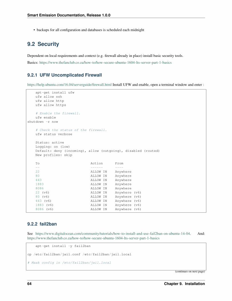
Smart Emission Documentation, Release 1.0.0
• backups for all configuration and databases is scheduled each midnight
9.2 Security
Dependent on local requirements and context (e.g. firewall already in place) install basic security tools.
Basics: https://www.thefanclub.co.za/how-to/how-secure-ubuntu-1604-lts-server-part-1-basics
9.2.1 UFW Uncomplicated Firewall
https://help.ubuntu.com/16.04/serverguide/firewall.html Install UFW and enable, open a terminal window and enter :
apt-get install ufwufw allow sshufw allow httpufw allow https
# Enable the firewall.ufw enable
shutdown -r now
# Check the status of the firewall.ufw status verbose
Status: activeLogging: on (low)Default: deny (incoming), allow (outgoing), disabled (routed)New profiles: skip
To Action From-- ------ ----22 ALLOW IN Anywhere80 ALLOW IN Anywhere443 ALLOW IN Anywhere1883 ALLOW IN Anywhere8086 ALLOW IN Anywhere22 (v6) ALLOW IN Anywhere (v6)80 (v6) ALLOW IN Anywhere (v6)443 (v6) ALLOW IN Anywhere (v6)1883 (v6) ALLOW IN Anywhere (v6)8086 (v6) ALLOW IN Anywhere (v6)
9.2.2 fail2ban
See https://www.digitalocean.com/community/tutorials/how-to-install-and-use-fail2ban-on-ubuntu-14-04. And:https://www.thefanclub.co.za/how-to/how-secure-ubuntu-1604-lts-server-part-1-basics
apt-get install -y fail2ban
cp /etc/fail2ban/jail.conf /etc/fail2ban/jail.local
# Maak config in /etc/fail2ban/jail.local
(continues on next page)
64 Chapter 9. Installation
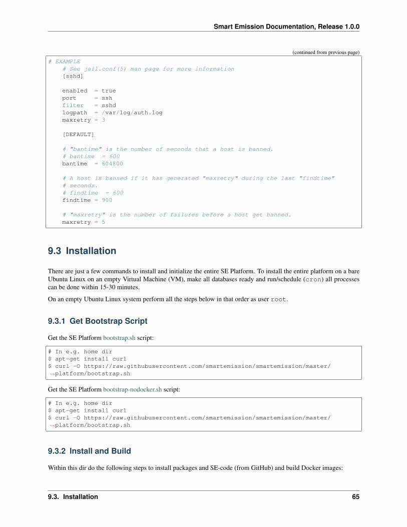
Smart Emission Documentation, Release 1.0.0
(continued from previous page)
# EXAMPLE# See jail.conf(5) man page for more information[sshd]
enabled = trueport = sshfilter = sshdlogpath = /var/log/auth.logmaxretry = 3
[DEFAULT]
# "bantime" is the number of seconds that a host is banned.# bantime = 600bantime = 604800
# A host is banned if it has generated "maxretry" during the last "findtime"# seconds.# findtime = 600findtime = 900
# "maxretry" is the number of failures before a host get banned.maxretry = 5
9.3 Installation
There are just a few commands to install and initialize the entire SE Platform. To install the entire platform on a bareUbuntu Linux on an empty Virtual Machine (VM), make all databases ready and run/schedule (cron) all processescan be done within 15-30 minutes.
On an empty Ubuntu Linux system perform all the steps below in that order as user root.
9.3.1 Get Bootstrap Script
Get the SE Platform bootstrap.sh script:
# In e.g. home dir$ apt-get install curl$ curl -O https://raw.githubusercontent.com/smartemission/smartemission/master/→˓platform/bootstrap.sh
Get the SE Platform bootstrap-nodocker.sh script:
# In e.g. home dir$ apt-get install curl$ curl -O https://raw.githubusercontent.com/smartemission/smartemission/master/→˓platform/bootstrap.sh
9.3.2 Install and Build
Within this dir do the following steps to install packages and SE-code (from GitHub) and build Docker images:
9.3. Installation 65
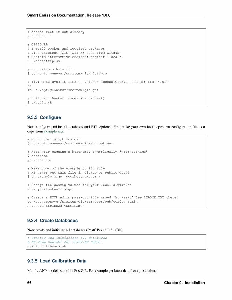
Smart Emission Documentation, Release 1.0.0
# become root if not already$ sudo su -
# OPTIONAL# Install Docker and required packages# plus checkout (Git) all SE code from GitHub# Confirm interactive choices: postfix "Local".$ ./bootstrap.sh
# go platform home dir:$ cd /opt/geonovum/smartem/git/platform
# Tip: make dynamic link to quickly access GitHub code dir from ~/gitcdln -s /opt/geonovum/smartem/git git
# build all Docker images (be patient)$ ./build.sh
9.3.3 Configure
Next configure and install databases and ETL-options. First make your own host-dependent configuration file as acopy from example.args:
# Go to config options dir$ cd /opt/geonovum/smartem/git/etl/options
# Note your machine's hostname, symbolically "yourhostname"$ hostnameyourhostname
# Make copy of the example config file# NB never put this file in GitHub or public dir!!$ cp example.args yourhostname.args
# Change the config values for your local situation$ vi yourhostname.args
# Create a HTTP admin password file named 'htpasswd' See README.TXT there.cd /opt/geonovum/smartem/git/services/web/config/adminhtpasswd htpasswd <username>
9.3.4 Create Databases
Now create and initialize all databases (PostGIS and InfluxDb):
# Creates and initializes all databases# NB WILL DESTROY ANY EXISTING DATA!!./init-databases.sh
9.3.5 Load Calibration Data
Mainly ANN models stored in PostGIS. For example get latest data from production:
66 Chapter 9. Installation
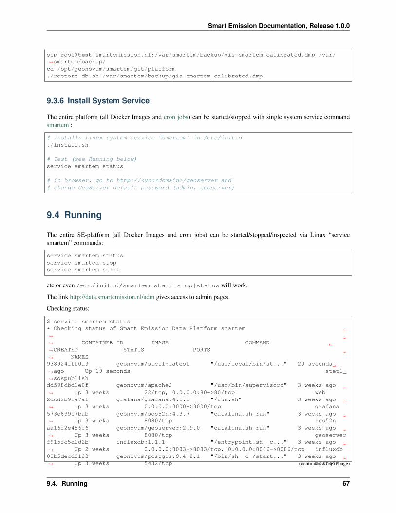
Smart Emission Documentation, Release 1.0.0
scp [email protected]:/var/smartem/backup/gis-smartem_calibrated.dmp /var/→˓smartem/backup/cd /opt/geonovum/smartem/git/platform./restore-db.sh /var/smartem/backup/gis-smartem_calibrated.dmp
9.3.6 Install System Service
The entire platform (all Docker Images and cron jobs) can be started/stopped with single system service commandsmartem :
# Installs Linux system service "smartem" in /etc/init.d./install.sh
# Test (see Running below)service smartem status
# in browser: go to http://<yourdomain>/geoserver and# change GeoServer default password (admin, geoserver)
9.4 Running
The entire SE-platform (all Docker Images and cron jobs) can be started/stopped/inspected via Linux “servicesmartem” commands:
service smartem statusservice smarted stopservice smartem start
etc or even /etc/init.d/smartem start|stop|status will work.
The link http://data.smartemission.nl/adm gives access to admin pages.
Checking status:
$ service smartem status
* Checking status of Smart Emission Data Platform smartem→˓
→˓ CONTAINER ID IMAGE COMMAND→˓CREATED STATUS PORTS→˓ NAMES938924fff0a3 geonovum/stetl:latest "/usr/local/bin/st..." 20 seconds→˓ago Up 19 seconds stetl_→˓sospublishdd598dbd1e0f geonovum/apache2 "/usr/bin/supervisord" 3 weeks ago→˓ Up 3 weeks 22/tcp, 0.0.0.0:80->80/tcp web2dcd2b91a7a1 grafana/grafana:4.1.1 "/run.sh" 3 weeks ago→˓ Up 3 weeks 0.0.0.0:3000->3000/tcp grafana573c839c7bab geonovum/sos52n:4.3.7 "catalina.sh run" 3 weeks ago→˓ Up 3 weeks 8080/tcp sos52naa16f2e456f6 geonovum/geoserver:2.9.0 "catalina.sh run" 3 weeks ago→˓ Up 3 weeks 8080/tcp geoserverf915fc5d1d2b influxdb:1.1.1 "/entrypoint.sh -c..." 3 weeks ago→˓ Up 2 weeks 0.0.0.0:8083->8083/tcp, 0.0.0.0:8086->8086/tcp influxdb08b5decd0123 geonovum/postgis:9.4-2.1 "/bin/sh -c /start..." 3 weeks ago→˓ Up 3 weeks 5432/tcp postgis(continues on next page)
9.4. Running 67

Smart Emission Documentation, Release 1.0.0
(continued from previous page)
# List cronjobs$ crontab -l
9.4.1 Handy Commands
Some handy Docker commands:
# cleanup non-running images$ sudo docker rm -v $(sudo docker ps -a -q -f status=exited)$ sudo docker rmi $(sudo docker images -f "dangling=true" -q)
# go into docker image named apache2 to bash promptsudo docker exec -it apache2 bash
# Find local Docker Bridge address of running containerdocker inspect --format '{{ .NetworkSettings.Networks.se_back.IPAddress }}' postgis# Example: psql to local postgis containerpsql -h `docker inspect --format '{{ .NetworkSettings.Networks.se_back.IPAddress }}'→˓postgis` -U docker -W gis
9.5 Docker Containers
Below the Docker Containers: how their generic Docker Images are built/acquired and how they are run using localmappings, data and configs.
Each Docker image build is found under /docker in GitHub. Docker Containers are run via subdirs underservices.
9.5.1 postgis - PostGIS Database
Uses PostGIS Docker image from Kartoza (Tim Sutton, QGIS lead), see https://hub.docker.com/r/kartoza/postgis/ andhttps://github.com/kartoza/docker-postgis .
This shorthand script run.sh will (re)run the postgis container.
#!/bin/bash## Run the Postgresql server with PostGIS and default database "gis".#
# Stop and remove possibly old containersdocker-compose stopdocker-compose rm -f
# Finally rundocker-compose up -d
# TIP to connect from host to postgis container# psql -h `sudo docker inspect --format '{{ .NetworkSettings.Networks.se_back.→˓IPAddress }}' postgis` -U docker -W gis
68 Chapter 9. Installation
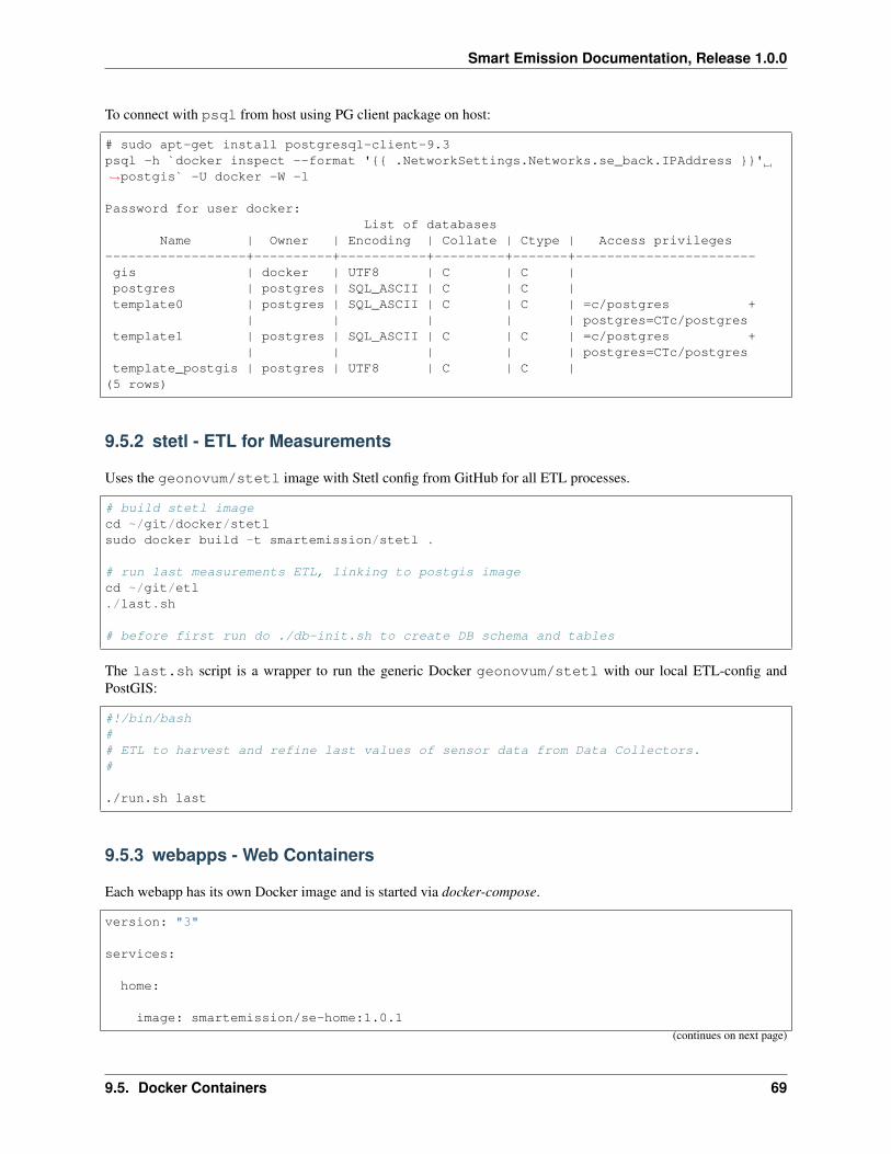
Smart Emission Documentation, Release 1.0.0
To connect with psql from host using PG client package on host:
# sudo apt-get install postgresql-client-9.3psql -h `docker inspect --format '{{ .NetworkSettings.Networks.se_back.IPAddress }}'→˓postgis` -U docker -W -l
Password for user docker:List of databases
Name | Owner | Encoding | Collate | Ctype | Access privileges------------------+----------+-----------+---------+-------+-----------------------gis | docker | UTF8 | C | C |postgres | postgres | SQL_ASCII | C | C |template0 | postgres | SQL_ASCII | C | C | =c/postgres +
| | | | | postgres=CTc/postgrestemplate1 | postgres | SQL_ASCII | C | C | =c/postgres +
| | | | | postgres=CTc/postgrestemplate_postgis | postgres | UTF8 | C | C |
(5 rows)
9.5.2 stetl - ETL for Measurements
Uses the geonovum/stetl image with Stetl config from GitHub for all ETL processes.
# build stetl imagecd ~/git/docker/stetlsudo docker build -t smartemission/stetl .
# run last measurements ETL, linking to postgis imagecd ~/git/etl./last.sh
# before first run do ./db-init.sh to create DB schema and tables
The last.sh script is a wrapper to run the generic Docker geonovum/stetl with our local ETL-config andPostGIS:
#!/bin/bash## ETL to harvest and refine last values of sensor data from Data Collectors.#
./run.sh last
9.5.3 webapps - Web Containers
Each webapp has its own Docker image and is started via docker-compose.
version: "3"
services:
home:
image: smartemission/se-home:1.0.1
(continues on next page)
9.5. Docker Containers 69
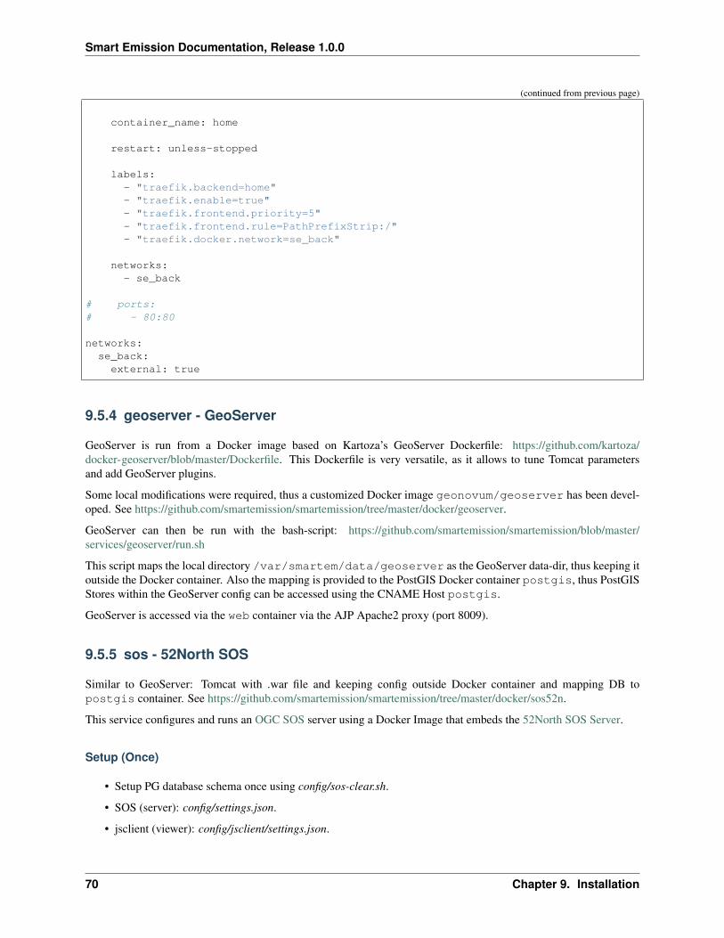
Smart Emission Documentation, Release 1.0.0
(continued from previous page)
container_name: home
restart: unless-stopped
labels:- "traefik.backend=home"- "traefik.enable=true"- "traefik.frontend.priority=5"- "traefik.frontend.rule=PathPrefixStrip:/"- "traefik.docker.network=se_back"
networks:- se_back
# ports:# - 80:80
networks:se_back:external: true
9.5.4 geoserver - GeoServer
GeoServer is run from a Docker image based on Kartoza’s GeoServer Dockerfile: https://github.com/kartoza/docker-geoserver/blob/master/Dockerfile. This Dockerfile is very versatile, as it allows to tune Tomcat parametersand add GeoServer plugins.
Some local modifications were required, thus a customized Docker image geonovum/geoserver has been devel-oped. See https://github.com/smartemission/smartemission/tree/master/docker/geoserver.
GeoServer can then be run with the bash-script: https://github.com/smartemission/smartemission/blob/master/services/geoserver/run.sh
This script maps the local directory /var/smartem/data/geoserver as the GeoServer data-dir, thus keeping itoutside the Docker container. Also the mapping is provided to the PostGIS Docker container postgis, thus PostGISStores within the GeoServer config can be accessed using the CNAME Host postgis.
GeoServer is accessed via the web container via the AJP Apache2 proxy (port 8009).
9.5.5 sos - 52North SOS
Similar to GeoServer: Tomcat with .war file and keeping config outside Docker container and mapping DB topostgis container. See https://github.com/smartemission/smartemission/tree/master/docker/sos52n.
This service configures and runs an OGC SOS server using a Docker Image that embeds the 52North SOS Server.
Setup (Once)
• Setup PG database schema once using config/sos-clear.sh.
• SOS (server): config/settings.json.
• jsclient (viewer): config/jsclient/settings.json.
70 Chapter 9. Installation
Smart Emission Documentation, Release 1.0.0
A sqlite DB contains all settings that can be managed via the GUI and is best copied from a previous configuredSOS instance in /var/smartem/data/sos52n/configuration.db. On the first start this dir will be created and linked usingDocker volume mapping.
9.5.6 gost - Geodan STA
This runs the Geodan GOST SensorThings API server. See the README there. Be sure to first create the PostGISDB schema for GOST.
See the bash-script how to run (no Docker-compose used!): https://github.com/smartemission/smartemission/blob/master/services/gost/run.sh .
9.5.7 influxdb - InfluxDB
This runs the InfluxDB service as a Docker container. See https://www.influxdata.com:
InfluxDB is an open source database written in Go specifically to handle time series data with high avail-ability and high performance requirements. InfluxDB installs in minutes without external dependencies,yet is flexible and scalable enough for complex deployments.
The Docker image comes from https://hub.docker.com/_/influxdb/
See https://github.com/smartemission/smartemission/tree/master/services/influxdb.
To be supplied further.
9.5.8 chronograf - Chronograf
This runs the Chronograf service as a Docker container. Chronograf is a visual admin tool for a.o. InfluxDB. Seehttps://www.influxdata.com:
Chronograf is a visualization tool for time series data in InfluxDB.
The Docker image comes from https://hub.docker.com/_/chronograf/
See https://github.com/smartemission/smartemission/tree/master/services/chronograf.
Only accessible via SE Admin web UI. To be supplied further.
9.5.9 grafana - Grafana
From http://grafana.org
“Grafana is an open source metric analytics and visualization suite. It is most commonly used for vi-sualizing time series data for infrastructure and application analytics but many use it in other domainsincluding industrial sensors, home automation, weather, and process control.”
Watch the demo and be amazed: http://play.grafana.org Documentation: http://docs.grafana.org
See https://github.com/smartemission/smartemission/tree/master/services/grafana.
To be supplied further.
9.5. Docker Containers 71

Smart Emission Documentation, Release 1.0.0
9.5.10 monitoring - Monitoring
Monitoring is based around Prometheus and a dedicated (for monitoring) Grafana instance. A complete monitoringstack is deployed via docker-compose based on the Docker Monitoring Project.
“Prometheus is an open-source systems monitoring and alerting toolkit originally built at SoundCloud.Since its inception in 2012, many companies and organizations have adopted Prometheus, and the projecthas a very active developer and user community. It is now a standalone open source project and maintainedindependently of any company. To emphasize this, and to clarify the project’s governance structure,Prometheus joined the Cloud Native Computing Foundation in 2016 as the second hosted project, afterKubernetes.”
Documentation: https://prometheus.io/docs/ . Howto: https://medium.com/@soumyadipde/monitoring-in-docker-stacks-its-that-easy-with-prometheus-5d71c1042443
See https://github.com/smartemission/smartemission/tree/master/services/monitoring.
The compose file is as follows:
# Adapted from Brian Christner's: https://github.com/vegasbrianc/prometheus# and later: https://github.com/vegasbrianc/docker-pulls/blob/master/docker-compose.→˓yml# All credits there!# Taken version-2 branch on dec 18, 2017.## Changes by Just van den Broecke:# - removed Docker Swarm stuff (why needed?)# - removed port mappings (prevent outside access)# - run on local bridge network (network_mode: bridge, as to be proxied from Apache→˓web container)
version: '3.1'
volumes:prometheus_data: {}grafana_data: {}
services:
node-exporter:# See https://github.com/vegasbrianc/docker-pulls/blob/master/docker-compose.ymlimage: prom/node-exportercontainer_name: node-exportervolumes:
- /proc:/host/proc:ro- /sys:/host/sys:ro- /:/rootfs:ro
command:- '--path.procfs=/host/proc'- '--path.sysfs=/host/sys'- --collector.filesystem.ignored-mount-points- "^/(sys|proc|dev|host|etc|rootfs/var/lib/docker/containers|rootfs/var/lib/
→˓docker/overlay2|rootfs/run/docker/netns|rootfs/var/lib/docker/aufs)($$|/)"# - '--collector.textfile.directory /etc/node-exporter/'# ports:# - 9100:9100
networks:- se_back
restart: unless-stopped(continues on next page)
72 Chapter 9. Installation
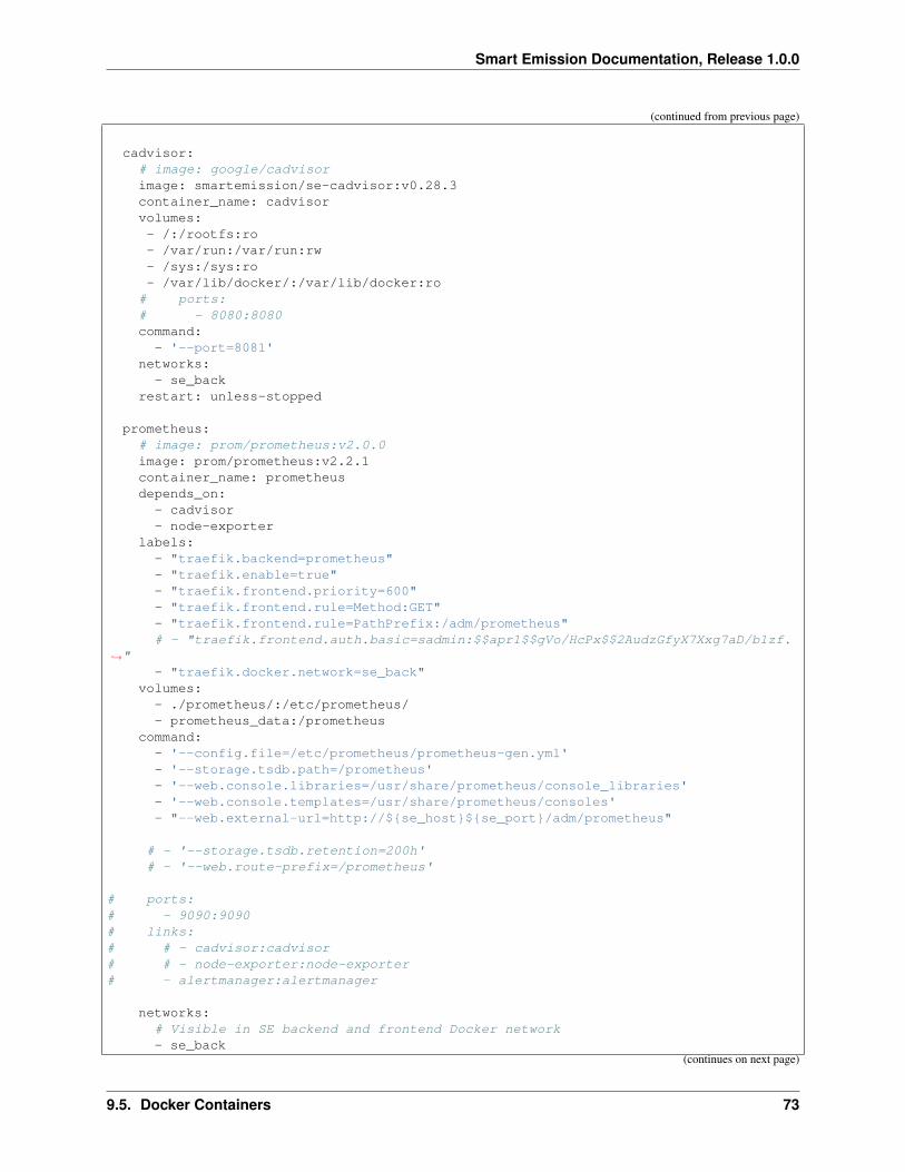
Smart Emission Documentation, Release 1.0.0
(continued from previous page)
cadvisor:# image: google/cadvisorimage: smartemission/se-cadvisor:v0.28.3container_name: cadvisorvolumes:- /:/rootfs:ro- /var/run:/var/run:rw- /sys:/sys:ro- /var/lib/docker/:/var/lib/docker:ro
# ports:# - 8080:8080command:
- '--port=8081'networks:
- se_backrestart: unless-stopped
prometheus:# image: prom/prometheus:v2.0.0image: prom/prometheus:v2.2.1container_name: prometheusdepends_on:
- cadvisor- node-exporter
labels:- "traefik.backend=prometheus"- "traefik.enable=true"- "traefik.frontend.priority=600"- "traefik.frontend.rule=Method:GET"- "traefik.frontend.rule=PathPrefix:/adm/prometheus"# - "traefik.frontend.auth.basic=sadmin:$$apr1$$gVo/HcPx$$2AudzGfyX7Xxg7aD/b1zf.
→˓"- "traefik.docker.network=se_back"
volumes:- ./prometheus/:/etc/prometheus/- prometheus_data:/prometheus
command:- '--config.file=/etc/prometheus/prometheus-gen.yml'- '--storage.tsdb.path=/prometheus'- '--web.console.libraries=/usr/share/prometheus/console_libraries'- '--web.console.templates=/usr/share/prometheus/consoles'- "--web.external-url=http://${se_host}${se_port}/adm/prometheus"
# - '--storage.tsdb.retention=200h'# - '--web.route-prefix=/prometheus'
# ports:# - 9090:9090# links:# # - cadvisor:cadvisor# # - node-exporter:node-exporter# - alertmanager:alertmanager
networks:# Visible in SE backend and frontend Docker network- se_back
(continues on next page)
9.5. Docker Containers 73
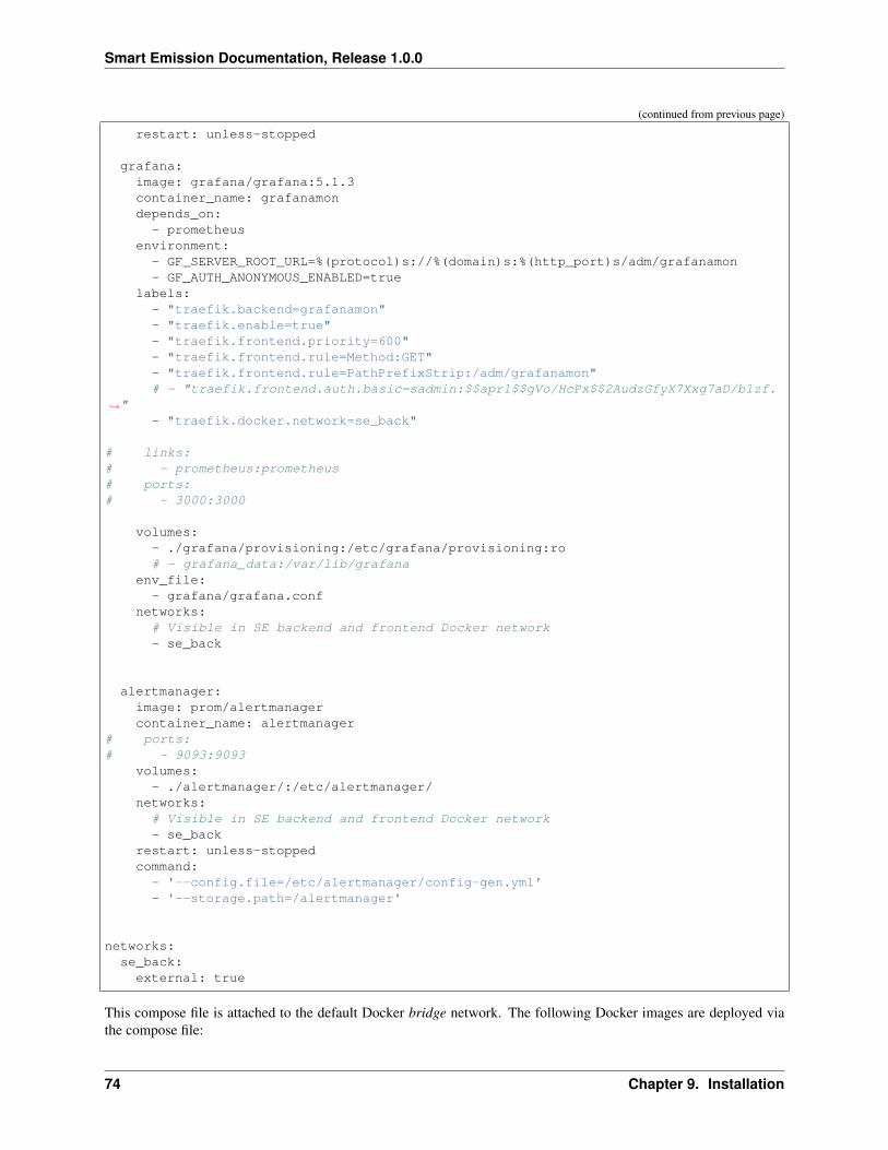
Smart Emission Documentation, Release 1.0.0
(continued from previous page)
restart: unless-stopped
grafana:image: grafana/grafana:5.1.3container_name: grafanamondepends_on:
- prometheusenvironment:
- GF_SERVER_ROOT_URL=%(protocol)s://%(domain)s:%(http_port)s/adm/grafanamon- GF_AUTH_ANONYMOUS_ENABLED=true
labels:- "traefik.backend=grafanamon"- "traefik.enable=true"- "traefik.frontend.priority=600"- "traefik.frontend.rule=Method:GET"- "traefik.frontend.rule=PathPrefixStrip:/adm/grafanamon"# - "traefik.frontend.auth.basic=sadmin:$$apr1$$gVo/HcPx$$2AudzGfyX7Xxg7aD/b1zf.
→˓"- "traefik.docker.network=se_back"
# links:# - prometheus:prometheus# ports:# - 3000:3000
volumes:- ./grafana/provisioning:/etc/grafana/provisioning:ro# - grafana_data:/var/lib/grafana
env_file:- grafana/grafana.conf
networks:# Visible in SE backend and frontend Docker network- se_back
alertmanager:image: prom/alertmanagercontainer_name: alertmanager
# ports:# - 9093:9093
volumes:- ./alertmanager/:/etc/alertmanager/
networks:# Visible in SE backend and frontend Docker network- se_back
restart: unless-stoppedcommand:
- '--config.file=/etc/alertmanager/config-gen.yml'- '--storage.path=/alertmanager'
networks:se_back:external: true
This compose file is attached to the default Docker bridge network. The following Docker images are deployed viathe compose file:
74 Chapter 9. Installation

Smart Emission Documentation, Release 1.0.0
Prometheus
Using Prometheus 2.0+. Configuration in prometheus.yml :
# my global configglobal:
scrape_interval: 15s # By default, scrape targets every 15 seconds.evaluation_interval: 15s # By default, scrape targets every 15 seconds.# scrape_timeout is set to the global default (10s).
# Attach these labels to any time series or alerts when communicating with# external systems (federation, remote storage, Alertmanager).external_labels:
monitor: 'smart-emission'
# Load and evaluate rules in this file every 'evaluation_interval' seconds.rule_files:
- 'alert.rules'# - "first.rules"# - "second.rules"
# alertalerting:
alertmanagers:- scheme: httpstatic_configs:- targets:
- "alertmanager:9093"
# A scrape configuration containing exactly one endpoint to scrape:# Here it's Prometheus itself.scrape_configs:
# The job name is added as a label `job=<job_name>` to any timeseries scraped from→˓this config.- job_name: 'prometheus'scrape_interval: 5shonor_labels: truemetrics_path: '/adm/prometheus/metrics'static_configs:
- targets: ['localhost:9090']
- job_name: 'node'
# Override the global default and scrape targets from this job every 5 seconds.scrape_interval: 5s
# metrics_path defaults to '/metrics'# scheme defaults to 'http'.
static_configs:- targets: ['$CADVISOR_HOST:8081','$NODE_EXPORTER_HOST:9100']
Secure and pass via Apache proxy:
<Location /adm/prometheus>ProxyPreserveHost OnProxyPass http://monitoring_prometheus_1:9090/adm/prometheusProxyPassReverse http://monitoring_prometheus_1:9090/adm/prometheus
(continues on next page)
9.5. Docker Containers 75

Smart Emission Documentation, Release 1.0.0
(continued from previous page)
RequestHeader unset Authorization</Location>
Grafana
Installed via docker-compose.
Secure and pass via Apache proxy:
<Location /adm/grafanamon>ProxyPreserveHost OnProxyPass http://monitoring_grafana_1:3000ProxyPassReverse http://monitoring_grafana_1:3000RequestHeader unset Authorization
</Location>
Add Prometheus with url http://prometheus:9090/adm/prometheus as DataSource with access proxy.
Import Dashboard 1860: https://grafana.com/dashboards/1860 to view Node Exporter stats. and 179: https://grafana.com/dashboards/179 to view Docker stats. Locally adapted versions of these are available under the /dashboards dir.Use the <name>-SE.json versions.
Alternative: https://github.com/stefanprodan/dockprom
cAdvisor
Used for getting metrics in Prometheus from Docker components. See https://github.com/google/cadvisor :
“cAdvisor (Container Advisor) provides container users an understanding of the resource usage and per-formance characteristics of their running containers. It is a running daemon that collects, aggregates,processes, and exports information about running containers. Specifically, for each container it keepsresource isolation parameters, historical resource usage, histograms of complete historical resource usageand network statistics. This data is exported by container and machine-wide.”
NB for now cAdvisor needs to be built because of this bug. Once that is resolved we can use official Docker Image.
NB cAdvisor via Docker on Ubuntu 14.04 has a serious issue (like Node_exporter) and this issue, so needs to beinstalled on host.
On Ubuntu 16.04 we can use cAdvisor in Docker again. Steps:
# Step 1: Install latest go-lang (go-lang package version on 14.04 too old!)# See https://github.com/golang/go/wiki/Ubuntu$ add-apt-repository ppa:gophers/archive$ apt update$ apt-get install golang-1.9-go$ ls /usr/lib/go-1.9/bin$ go gofmt$ export GOROOT=/usr/lib/go-1.9$ export PATH=$GOROOT/bin:$PATH
# Step 2 cAdvisor build# See https://github.com/google/cadvisor/blob/master/docs/development/build.md$ mkdir /opt/cadvisor$ cd /opt/cadvisor$ export GOPATH=/opt/cadvisor
(continues on next page)
76 Chapter 9. Installation

Smart Emission Documentation, Release 1.0.0
(continued from previous page)
$ go get -d github.com/google/cadvisor$ cd /opt/cadvisor/src/github.com/google/cadvisor$ make build$ make test (fails somehow)$ ./cadvisor -version
cAdvisor version v0.28.3.2+9ffa37396f19cb (9ffa373)$ ./cadvisor# surf to host:8080
# Step 3: install supervisord$ apt-get install supervisor$ service supervisor status
is running
# Step 4: cAdvisor as supervisrod process (conf)# See https://github.com/google/cadvisor/issues/771#issuecomment-322725681
# Put in /etc/supervisor/conf.d/cadvisor.conf[program:cadvisor]directory=/opt/geonovum/smartem/git/services/monitoring/cadvisorcommand=/opt/geonovum/smartem/git/services/monitoring/cadvisor/run.shautostart=trueautorestart=unexpectedredirect_stderr=true
# with /opt/geonovum/smartem/git/services/monitoring/cadvisor/run.sh# NB ENV setting via supervisord did not work on this version, need supervisor 3.2#!/bin/bash#export PARENT_HOST=`ip route show | grep docker0 | awk '{print \$9}'`export GOROOT="/usr/lib/go-1.9"export GOPATH="/opt/cadvisor/src/github.com/google/cadvisor"export PATH="${GOPATH}:${GOROOT}/bin:${PATH}"
cd ${GOPATH}./cadvisor -listen_ip ${PARENT_HOST} -port 8080
# run$ service supervisor stop$ service supervisor start# Check via host port 8080 and:$ ps -elf | grep cadvisor
4 S.... 00:00:01 /opt/cadvisor/src/github.com/google/cadvisor/cadvisor -port 8080
Node Exporter
In Grafana import Dashboard 1860: https://grafana.com/dashboards/1860 to view Node Exporter stats.
Node Exporter can be installed on the host to gather Linux/Ubuntu metrics.
Steps to install in /usr/bin/node_exporter:
mkdir -p /var/smartem/prometheus/archivecd /var/smartem/prometheus/archivewget https://github.com/prometheus/node_exporter/releases/download/v0.15.2/node_→˓exporter-0.15.2.linux-amd64.tar.gz
(continues on next page)
9.5. Docker Containers 77
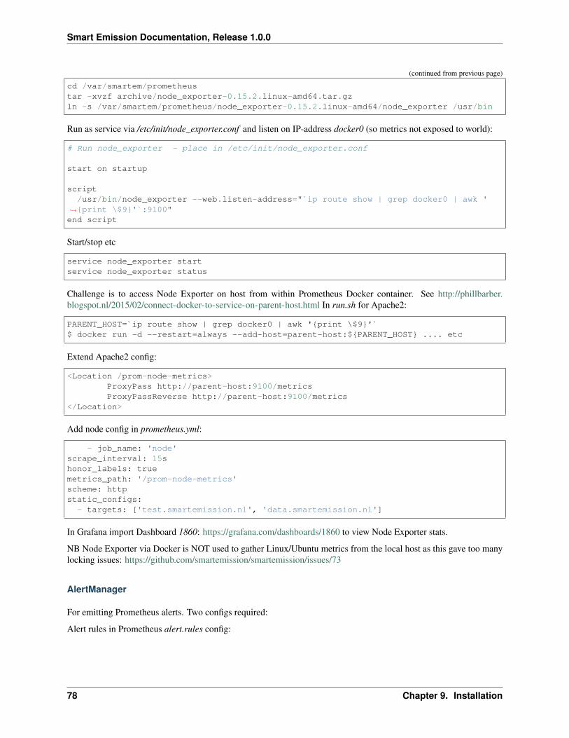
Smart Emission Documentation, Release 1.0.0
(continued from previous page)
cd /var/smartem/prometheustar -xvzf archive/node_exporter-0.15.2.linux-amd64.tar.gzln -s /var/smartem/prometheus/node_exporter-0.15.2.linux-amd64/node_exporter /usr/bin
Run as service via /etc/init/node_exporter.conf and listen on IP-address docker0 (so metrics not exposed to world):
# Run node_exporter - place in /etc/init/node_exporter.conf
start on startup
script/usr/bin/node_exporter --web.listen-address="`ip route show | grep docker0 | awk '
→˓{print \$9}'`:9100"end script
Start/stop etc
service node_exporter startservice node_exporter status
Challenge is to access Node Exporter on host from within Prometheus Docker container. See http://phillbarber.blogspot.nl/2015/02/connect-docker-to-service-on-parent-host.html In run.sh for Apache2:
PARENT_HOST=`ip route show | grep docker0 | awk '{print \$9}'`$ docker run -d --restart=always --add-host=parent-host:${PARENT_HOST} .... etc
Extend Apache2 config:
<Location /prom-node-metrics>ProxyPass http://parent-host:9100/metricsProxyPassReverse http://parent-host:9100/metrics
</Location>
Add node config in prometheus.yml:
- job_name: 'node'scrape_interval: 15shonor_labels: truemetrics_path: '/prom-node-metrics'scheme: httpstatic_configs:
- targets: ['test.smartemission.nl', 'data.smartemission.nl']
In Grafana import Dashboard 1860: https://grafana.com/dashboards/1860 to view Node Exporter stats.
NB Node Exporter via Docker is NOT used to gather Linux/Ubuntu metrics from the local host as this gave too manylocking issues: https://github.com/smartemission/smartemission/issues/73
AlertManager
For emitting Prometheus alerts. Two configs required:
Alert rules in Prometheus alert.rules config:
78 Chapter 9. Installation
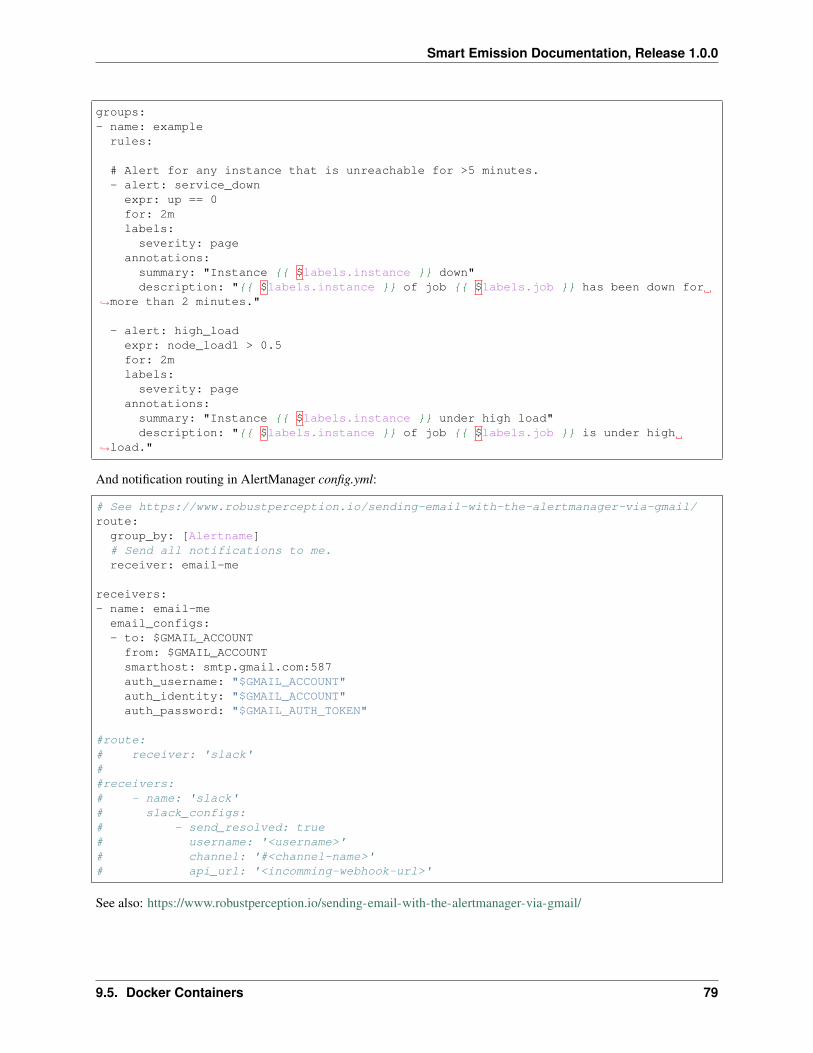
Smart Emission Documentation, Release 1.0.0
groups:- name: example
rules:
# Alert for any instance that is unreachable for >5 minutes.- alert: service_downexpr: up == 0for: 2mlabels:
severity: pageannotations:
summary: "Instance {{ $labels.instance }} down"description: "{{ $labels.instance }} of job {{ $labels.job }} has been down for
→˓more than 2 minutes."
- alert: high_loadexpr: node_load1 > 0.5for: 2mlabels:
severity: pageannotations:
summary: "Instance {{ $labels.instance }} under high load"description: "{{ $labels.instance }} of job {{ $labels.job }} is under high
→˓load."
And notification routing in AlertManager config.yml:
# See https://www.robustperception.io/sending-email-with-the-alertmanager-via-gmail/route:
group_by: [Alertname]# Send all notifications to me.receiver: email-me
receivers:- name: email-me
email_configs:- to: $GMAIL_ACCOUNTfrom: $GMAIL_ACCOUNTsmarthost: smtp.gmail.com:587auth_username: "$GMAIL_ACCOUNT"auth_identity: "$GMAIL_ACCOUNT"auth_password: "$GMAIL_AUTH_TOKEN"
#route:# receiver: 'slack'##receivers:# - name: 'slack'# slack_configs:# - send_resolved: true# username: '<username>'# channel: '#<channel-name>'# api_url: '<incomming-webhook-url>'
See also: https://www.robustperception.io/sending-email-with-the-alertmanager-via-gmail/
9.5. Docker Containers 79
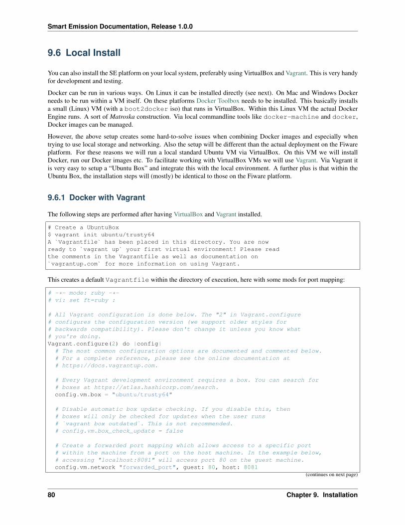
Smart Emission Documentation, Release 1.0.0
9.6 Local Install
You can also install the SE platform on your local system, preferably using VirtualBox and Vagrant. This is very handyfor development and testing.
Docker can be run in various ways. On Linux it can be installed directly (see next). On Mac and Windows Dockerneeds to be run within a VM itself. On these platforms Docker Toolbox needs to be installed. This basically installsa small (Linux) VM (with a boot2docker iso) that runs in VirtualBox. Within this Linux VM the actual DockerEngine runs. A sort of Matroska construction. Via local commandline tools like docker-machine and docker,Docker images can be managed.
However, the above setup creates some hard-to-solve issues when combining Docker images and especially whentrying to use local storage and networking. Also the setup will be different than the actual deployment on the Fiwareplatform. For these reasons we will run a local standard Ubuntu VM via VirtualBox. On this VM we will installDocker, run our Docker images etc. To facilitate working with VirtualBox VMs we will use Vagrant. Via Vagrant itis very easy to setup a “Ubuntu Box” and integrate this with the local environment. A further plus is that within theUbuntu Box, the installation steps will (mostly) be identical to those on the Fiware platform.
9.6.1 Docker with Vagrant
The following steps are performed after having VirtualBox and Vagrant installed.
# Create a UbuntuBox$ vagrant init ubuntu/trusty64A `Vagrantfile` has been placed in this directory. You are nowready to `vagrant up` your first virtual environment! Please readthe comments in the Vagrantfile as well as documentation on`vagrantup.com` for more information on using Vagrant.
This creates a default Vagrantfile within the directory of execution, here with some mods for port mapping:
# -*- mode: ruby -*-# vi: set ft=ruby :
# All Vagrant configuration is done below. The "2" in Vagrant.configure# configures the configuration version (we support older styles for# backwards compatibility). Please don't change it unless you know what# you're doing.Vagrant.configure(2) do |config|
# The most common configuration options are documented and commented below.# For a complete reference, please see the online documentation at# https://docs.vagrantup.com.
# Every Vagrant development environment requires a box. You can search for# boxes at https://atlas.hashicorp.com/search.config.vm.box = "ubuntu/trusty64"
# Disable automatic box update checking. If you disable this, then# boxes will only be checked for updates when the user runs# `vagrant box outdated`. This is not recommended.# config.vm.box_check_update = false
# Create a forwarded port mapping which allows access to a specific port# within the machine from a port on the host machine. In the example below,# accessing "localhost:8081" will access port 80 on the guest machine.config.vm.network "forwarded_port", guest: 80, host: 8081
(continues on next page)
80 Chapter 9. Installation
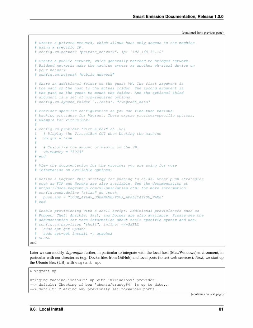
Smart Emission Documentation, Release 1.0.0
(continued from previous page)
# Create a private network, which allows host-only access to the machine# using a specific IP.# config.vm.network "private_network", ip: "192.168.33.10"
# Create a public network, which generally matched to bridged network.# Bridged networks make the machine appear as another physical device on# your network.# config.vm.network "public_network"
# Share an additional folder to the guest VM. The first argument is# the path on the host to the actual folder. The second argument is# the path on the guest to mount the folder. And the optional third# argument is a set of non-required options.# config.vm.synced_folder "../data", "/vagrant_data"
# Provider-specific configuration so you can fine-tune various# backing providers for Vagrant. These expose provider-specific options.# Example for VirtualBox:## config.vm.provider "virtualbox" do |vb|# # Display the VirtualBox GUI when booting the machine# vb.gui = true## # Customize the amount of memory on the VM:# vb.memory = "1024"# end## View the documentation for the provider you are using for more# information on available options.
# Define a Vagrant Push strategy for pushing to Atlas. Other push strategies# such as FTP and Heroku are also available. See the documentation at# https://docs.vagrantup.com/v2/push/atlas.html for more information.# config.push.define "atlas" do |push|# push.app = "YOUR_ATLAS_USERNAME/YOUR_APPLICATION_NAME"# end
# Enable provisioning with a shell script. Additional provisioners such as# Puppet, Chef, Ansible, Salt, and Docker are also available. Please see the# documentation for more information about their specific syntax and use.# config.vm.provision "shell", inline: <<-SHELL# sudo apt-get update# sudo apt-get install -y apache2# SHELL
end
Later we can modify Vagrantfile further, in particular to integrate with the local host (Mac/Windows) environment, inparticular with our directories (e.g. Dockerfiles from GitHub) and local ports (to test web services). Next, we start upthe Ubuntu Box (UB) with vagrant up:
$ vagrant up
Bringing machine 'default' up with 'virtualbox' provider...==> default: Checking if box 'ubuntu/trusty64' is up to date...==> default: Clearing any previously set forwarded ports...
(continues on next page)
9.6. Local Install 81

Smart Emission Documentation, Release 1.0.0
(continued from previous page)
==> default: Clearing any previously set network interfaces...==> default: Preparing network interfaces based on configuration...
default: Adapter 1: nat==> default: Forwarding ports...
default: 22 (guest) => 2222 (host) (adapter 1)==> default: Booting VM...==> default: Waiting for machine to boot. This may take a few minutes...
default: SSH address: 127.0.0.1:2222default: SSH username: vagrantdefault: SSH auth method: private keydefault: Warning: Remote connection disconnect. Retrying...default: Warning: Remote connection disconnect. Retrying...
==> default: Machine booted and ready!
We see that SSH port 22 is mapped to localhost:2222. Login to the box:
ssh -p 2222 vagrant@localhost # password vagrant
# but easier is to use vagrantvagrant ssh
Our local directory is also automatically mounted in the UB so we can have access to our development files (inGitHub):
vagrant@vagrant-ubuntu-trusty-64:~$ ls /vagrant/contrib data doc git Vagrantfile
# and our Dockerfiles within GitHubvagrant@vagrant-ubuntu-trusty-64:~$ ls /vagrant/git/dockerapache2 boot2docker-fw.sh postgis stetl
Within the UB we are on a standard Ubuntu commandline, running a general Ubuntu upgrade first:
$ sudo apt-get update$ sudo apt-get -y upgrade
The next steps are standard Docker install (see next section below). After the setup is tested by building and runningone of our Docker files. Getting access to our Dockerfiles is easy, for example:
sudo ln -s /vagrant/git ~/gitcd ~/git/docker/apache2sudo docker build -t geonovum/apache2 .
Run and test:
sudo docker run -p 2222:22 -p 80:80 -t -i geonovum/apache2
Then access Apache from local system via localhost:8081.
Same for Stetl, build and test:
$ cd ~/git/docker/stetl$ sudo docker build -t smartemission/stetl .$ cd test/1_copystd$ sudo docker run -v `pwd`:`pwd` -w `pwd` -t -i geonovum/stetl -c etl.cfg
(continues on next page)
82 Chapter 9. Installation

Smart Emission Documentation, Release 1.0.0
Fig. 1: Access Apache running with Docker externally
9.6. Local Install 83
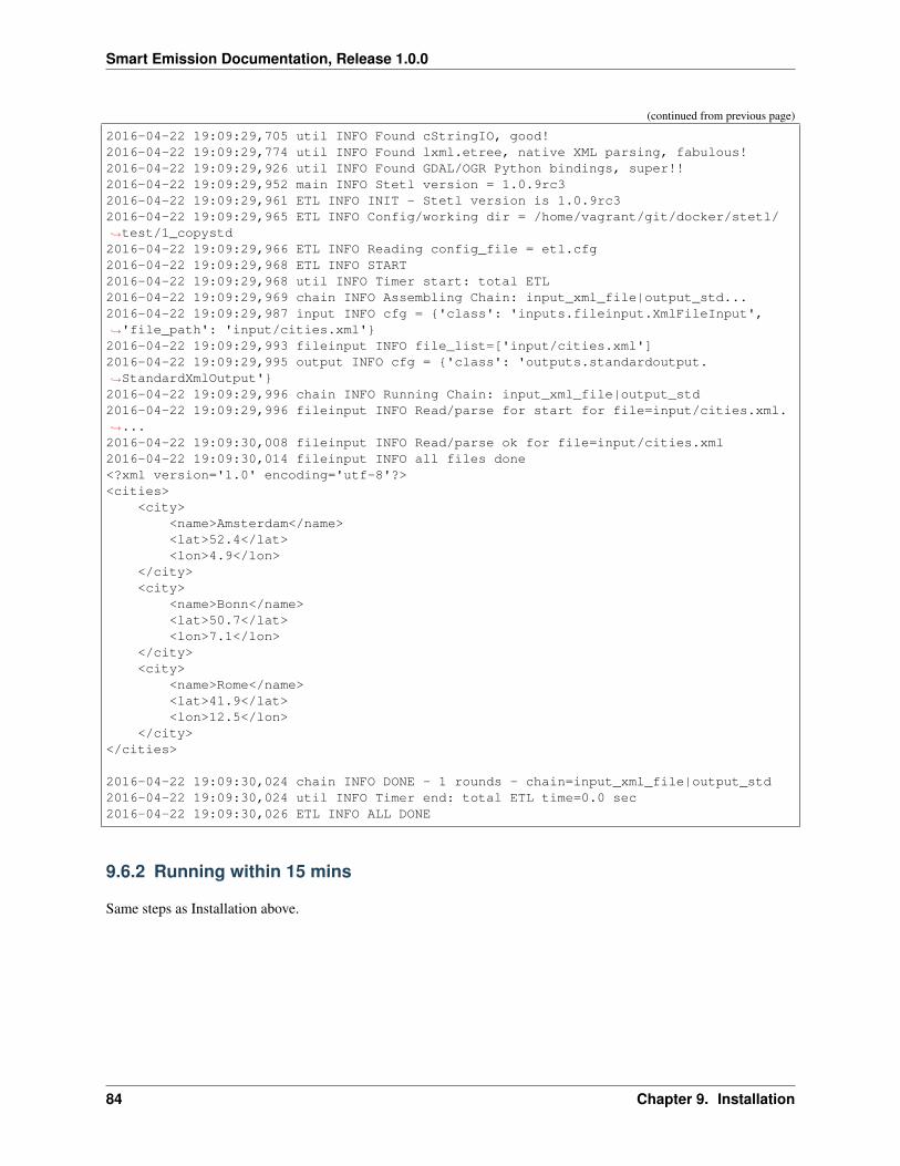
Smart Emission Documentation, Release 1.0.0
(continued from previous page)
2016-04-22 19:09:29,705 util INFO Found cStringIO, good!2016-04-22 19:09:29,774 util INFO Found lxml.etree, native XML parsing, fabulous!2016-04-22 19:09:29,926 util INFO Found GDAL/OGR Python bindings, super!!2016-04-22 19:09:29,952 main INFO Stetl version = 1.0.9rc32016-04-22 19:09:29,961 ETL INFO INIT - Stetl version is 1.0.9rc32016-04-22 19:09:29,965 ETL INFO Config/working dir = /home/vagrant/git/docker/stetl/→˓test/1_copystd2016-04-22 19:09:29,966 ETL INFO Reading config_file = etl.cfg2016-04-22 19:09:29,968 ETL INFO START2016-04-22 19:09:29,968 util INFO Timer start: total ETL2016-04-22 19:09:29,969 chain INFO Assembling Chain: input_xml_file|output_std...2016-04-22 19:09:29,987 input INFO cfg = {'class': 'inputs.fileinput.XmlFileInput',→˓'file_path': 'input/cities.xml'}2016-04-22 19:09:29,993 fileinput INFO file_list=['input/cities.xml']2016-04-22 19:09:29,995 output INFO cfg = {'class': 'outputs.standardoutput.→˓StandardXmlOutput'}2016-04-22 19:09:29,996 chain INFO Running Chain: input_xml_file|output_std2016-04-22 19:09:29,996 fileinput INFO Read/parse for start for file=input/cities.xml.→˓...2016-04-22 19:09:30,008 fileinput INFO Read/parse ok for file=input/cities.xml2016-04-22 19:09:30,014 fileinput INFO all files done<?xml version='1.0' encoding='utf-8'?><cities>
<city><name>Amsterdam</name><lat>52.4</lat><lon>4.9</lon>
</city><city>
<name>Bonn</name><lat>50.7</lat><lon>7.1</lon>
</city><city>
<name>Rome</name><lat>41.9</lat><lon>12.5</lon>
</city></cities>
2016-04-22 19:09:30,024 chain INFO DONE - 1 rounds - chain=input_xml_file|output_std2016-04-22 19:09:30,024 util INFO Timer end: total ETL time=0.0 sec2016-04-22 19:09:30,026 ETL INFO ALL DONE
9.6.2 Running within 15 mins
Same steps as Installation above.
84 Chapter 9. Installation
CHAPTER 10
Kubernetes
This chapter describes the installation and maintenance for the Smart Emission Data Platform in a Kubernetes (K8s)environment. Note that installation and maintenance in a Docker environment is described in the Installation chapter.SE was initially (2016-2018) deployed as Containers on a single “bare Docker” machine. Later with the use of docker-compose and Docker Hub but still “bare Docker”. In spring 2018 migration within Kadaster-PDOK to K8s started,deploying in the K8s environment on Azure.
10.1 Principles
These are requirements and principles to understand and install an instance of the SE platform. It is required to havean understanding of Docker a nd Kubernetes (K8s) as that is the main environment in which the SE Platform is run.
Most Smart Emission services are deployed as follows in K8s:
• deployment.yml - specifies (Pods for) a K8s Deployment
• service.yml - describes a K8s Service (internal network proxy access) for the Pods in the Deployment
• ingress.yml - rules how to route outside requests to Service (only if the Service requires outside access)
Only for InfluxDB instances, as it requires local storage a StatefulSet is deployed i.s.o. a regular Deployment.
Postgres/PostGIS is not deployed within K8s but accessed as an external Azure Database for PostgreSQL serverservice from MS Azure.
10.2 Install
Install clients.
10.2.1 Ubuntu
As follows:
85
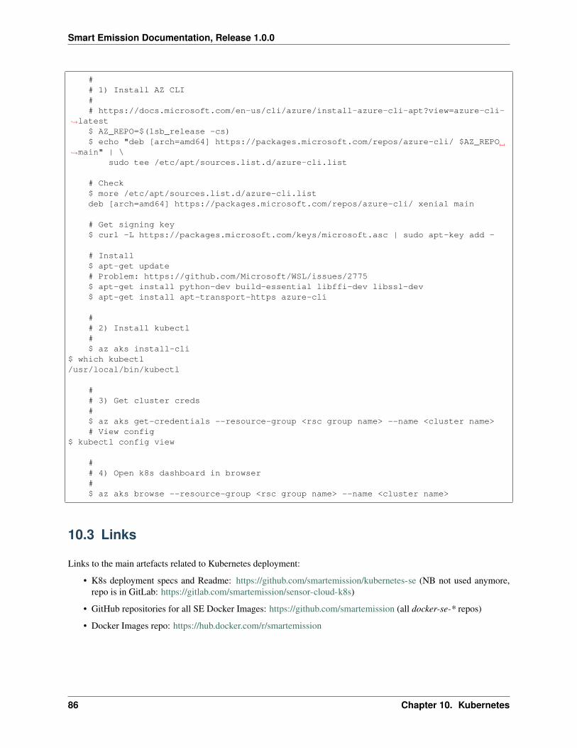
Smart Emission Documentation, Release 1.0.0
## 1) Install AZ CLI## https://docs.microsoft.com/en-us/cli/azure/install-azure-cli-apt?view=azure-cli-
→˓latest$ AZ_REPO=$(lsb_release -cs)$ echo "deb [arch=amd64] https://packages.microsoft.com/repos/azure-cli/ $AZ_REPO
→˓main" | \sudo tee /etc/apt/sources.list.d/azure-cli.list
# Check$ more /etc/apt/sources.list.d/azure-cli.listdeb [arch=amd64] https://packages.microsoft.com/repos/azure-cli/ xenial main
# Get signing key$ curl -L https://packages.microsoft.com/keys/microsoft.asc | sudo apt-key add -
# Install$ apt-get update# Problem: https://github.com/Microsoft/WSL/issues/2775$ apt-get install python-dev build-essential libffi-dev libssl-dev$ apt-get install apt-transport-https azure-cli
## 2) Install kubectl#$ az aks install-cli
$ which kubectl/usr/local/bin/kubectl
## 3) Get cluster creds#$ az aks get-credentials --resource-group <rsc group name> --name <cluster name># View config
$ kubectl config view
## 4) Open k8s dashboard in browser#$ az aks browse --resource-group <rsc group name> --name <cluster name>
10.3 Links
Links to the main artefacts related to Kubernetes deployment:
• K8s deployment specs and Readme: https://github.com/smartemission/kubernetes-se (NB not used anymore,repo is in GitLab: https://gitlab.com/smartemission/sensor-cloud-k8s)
• GitHub repositories for all SE Docker Images: https://github.com/smartemission (all docker-se-* repos)
• Docker Images repo: https://hub.docker.com/r/smartemission
86 Chapter 10. Kubernetes
Smart Emission Documentation, Release 1.0.0
10.4 Setup
Setting up local environment to interact with K8s cluster on Azure.
10.4.1 Mac OSX
Using Homebrew. Need to install kubernetes-cli and az-cli:
$ brew install azure-cli
$ brew install kubernetes-cli
10.5 Updating
For Deployments, CronJobs, StatefulSets, the current sequence of actions to roll out new updates for code or configchanges in Docker Images, is as follows (pre-CI/CD):
• make code changes in related GH repo, e.g docker-se-stetl for ETL changes
• increase the GH tag number: git tag to list current tags, then: git tag <new version nr> and git push –tags
• add a new build with the tag just added for this component in SmartEmission Organisation in DockerHub, e.g.smartemission/se-stetl
• trigger the build there in DockerHub, wait until build finished and succesful
• increase version number in the Deployment YAML, e.g. the GeoServer deployment.yml
• upgrade current Deployment (or Cronjob StatefulSet) to the Cluster kubectl -n smartemission replace -f deploy-ment.yml
• follow in K8s Dashboard or with kubectl for any errors
(TODO: automate this via Jenkins or some CI/CD tooling).
10.6 Namespaces
The main two operational K8s Namespaces are:
• smartemission - the main SE service stack and ETL
• collectors - Data Collector services and Dashboards (see global Architecture Chapter)
Additional, supporting, Namespaces are:
• monitoring - Monitoring related
• cert-manager - (Let’s Encrypt) SSL certificate management
• ingress-nginx - Ingress services based on nginx-proxying (external/public access)
• kube-system - mainly K8s Dashboard related
10.4. Setup 87
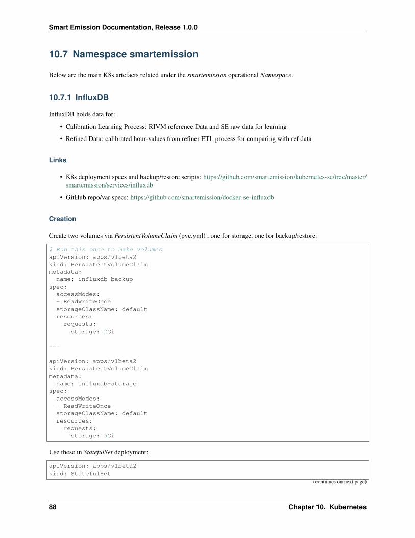
Smart Emission Documentation, Release 1.0.0
10.7 Namespace smartemission
Below are the main K8s artefacts related under the smartemission operational Namespace.
10.7.1 InfluxDB
InfluxDB holds data for:
• Calibration Learning Process: RIVM reference Data and SE raw data for learning
• Refined Data: calibrated hour-values from refiner ETL process for comparing with ref data
Links
• K8s deployment specs and backup/restore scripts: https://github.com/smartemission/kubernetes-se/tree/master/smartemission/services/influxdb
• GitHub repo/var specs: https://github.com/smartemission/docker-se-influxdb
Creation
Create two volumes via PersistentVolumeClaim (pvc.yml) , one for storage, one for backup/restore:
# Run this once to make volumesapiVersion: apps/v1beta2kind: PersistentVolumeClaimmetadata:
name: influxdb-backupspec:
accessModes:- ReadWriteOncestorageClassName: defaultresources:requests:
storage: 2Gi
---
apiVersion: apps/v1beta2kind: PersistentVolumeClaimmetadata:
name: influxdb-storagespec:
accessModes:- ReadWriteOncestorageClassName: defaultresources:requests:
storage: 5Gi
Use these in StatefulSet deployment:
apiVersion: apps/v1beta2kind: StatefulSet
(continues on next page)
88 Chapter 10. Kubernetes
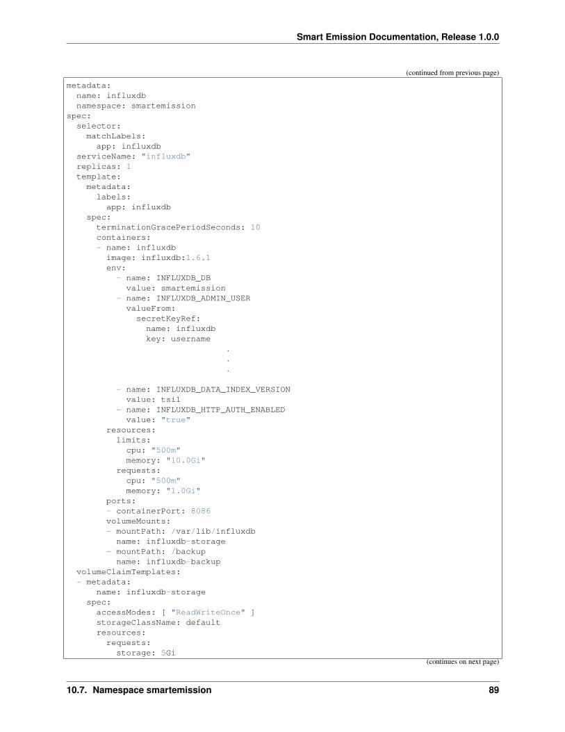
Smart Emission Documentation, Release 1.0.0
(continued from previous page)
metadata:name: influxdbnamespace: smartemission
spec:selector:matchLabels:
app: influxdbserviceName: "influxdb"replicas: 1template:metadata:
labels:app: influxdb
spec:terminationGracePeriodSeconds: 10containers:- name: influxdb
image: influxdb:1.6.1env:- name: INFLUXDB_DBvalue: smartemission
- name: INFLUXDB_ADMIN_USERvalueFrom:secretKeyRef:name: influxdbkey: username
.
.
.
- name: INFLUXDB_DATA_INDEX_VERSIONvalue: tsi1
- name: INFLUXDB_HTTP_AUTH_ENABLEDvalue: "true"
resources:limits:cpu: "500m"memory: "10.0Gi"
requests:cpu: "500m"memory: "1.0Gi"
ports:- containerPort: 8086volumeMounts:- mountPath: /var/lib/influxdbname: influxdb-storage
- mountPath: /backupname: influxdb-backup
volumeClaimTemplates:- metadata:
name: influxdb-storagespec:
accessModes: [ "ReadWriteOnce" ]storageClassName: defaultresources:
requests:storage: 5Gi
(continues on next page)
10.7. Namespace smartemission 89
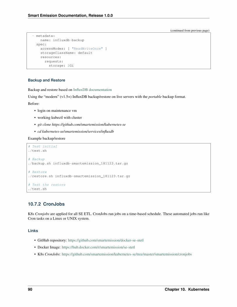
Smart Emission Documentation, Release 1.0.0
(continued from previous page)
- metadata:name: influxdb-backup
spec:accessModes: [ "ReadWriteOnce" ]storageClassName: defaultresources:
requests:storage: 2Gi
Backup and Restore
Backup and restore based on InfluxDB documentation
Using the “modern” (v1.5+) InfluxDB backup/restore on live servers with the portable backup format.
Before:
• login on maintenance vm
• working kubectl with cluster
• git clone https://github.com/smartemission/kubernetes-se
• cd kubernetes-se/smartemission/services/influxdb
Example backup/restore
# Test initial./test.sh
# Backup./backup.sh influxdb-smartemission_181123.tar.gz
# Restore./restore.sh influxdb-smartemission_181123.tar.gz
# Test the restore./test.sh
10.7.2 CronJobs
K8s Cronjobs are applied for all SE ETL. CronJobs run jobs on a time-based schedule. These automated jobs run likeCron tasks on a Linux or UNIX system.
Links
• GitHub repository: https://github.com/smartemission/docker-se-stetl
• Docker Image: https://hub.docker.com/r/smartemission/se-stetl
• K8s CronJobs: https://github.com/smartemission/kubernetes-se/tree/master/smartemission/cronjobs
90 Chapter 10. Kubernetes
Smart Emission Documentation, Release 1.0.0
Implementation
All ETL is based on the Stetl ETL framework. A single Docker Image based on the official Stetl Docker Imagecontains all ETL processes. A start-up parameter determines the specific ETL process to run. Design of the ETL isdescribed in the Data Management chapter.
10.7. Namespace smartemission 91

Smart Emission Documentation, Release 1.0.0
92 Chapter 10. Kubernetes
CHAPTER 11
Sensors
Originally the SE Platform was developed for a single sensor device (station), the Intemo Jose(ne). As time moved onadditional sensor devices from various sensor projects were integrated, or are in progress. To allow for multiple sensorstations/devices, each with multiple internal sensors from multiple projects, internals for mainly the ETL processes(cron jobs) were generalized while still keeping the core principles of the overall architecture and multi-step ETLprocessing: raw data harvesting (pull), refinement (validation, calibration), service-publication.
Based on device/sensor-types different ETL algorithms need to be applied. For example, some devices already emitcalibrated sensor-values (Luftdaten, Osiris), others require ANN calibration (Jose), others even per-sensor linear orpolynominal equations, sometimes per-sensor (AirSensEUR AlphaSense).
The advantage of the current approach is that once measurements are ‘in’, they become automatically available throughall external APIs without any additional action. Only on the ‘input’ (harvesting)-side and refinement ETL are specificformatting steps required.
11.1 Principles
To integrate a new sensor station type, two main items need to be resolved:
• APIs from which sensor-data can be harvested (‘getting the raw or sometimes calibrated data in’)
• amount/complexity of calibration and validation needed
In addition, a sensor station type is usually related to a Project. In an early stage every device was given a uniqueid, where the first 4 digits is the project id, followed by additional digits, denoting the station id within that project.Sometimes a mapping is required. The original station id is always kept in metadata columns.
11.1.1 APIs
Data from sensors is never sent directly to the SE platform. It is sent to what are called Data Collectors. These areusually not maintained by SE but by the specific projects like Smart City Living Lab, Luftdaten and/or companies likeIntemo etc. The only requirement is that these Data Collectors provide APIs for pulling data into (Harvesting) the SEPlatform.
93
Smart Emission Documentation, Release 1.0.0
Currently, harvesting from three Data Collector APIs has been realized:
1. Raw Sensor (a.k.a. Whale) API from now mainly Intemo (Jose stations) servers
2. InfluxDB Data Collector API, now mainly for AirSensEUR stations
3. Luftdaten API, for Luftdaten.info kits
Ad 2) this InfluxDB API is maintained by the SE Project itself and may be used in later projects to publish (push) datafrom additional sensors.
11.1.2 Calibration
Currently, the following calibration algorithms are implemented:
1. Jose stations: ANN Calibration
2. AirSensEUR per-sensor linear or polynominal equations
3. Luftdaten.info : no calibration required
These algorithms are reusable, mainly the parameters for each need to be set.
So how is this realized internally? Basic principles:
• while harvesting as much metadata as possible is extracted or configured
• the programming concept of an abstract Device and Device registry
Each station-type (Jose, ASE, Luftdaten) is mapped to a Device Type. From there, specific processing, configurationand algorithms are invoked. A special Device Type is the Vanilla Device. The Vanilla Device Type can be used whenno specific calibration is required. This is the easiest way to attach stations and was introduced when attaching kitsfrom the Luftdaten Project .
Each Device has one to three additional items/files:
• Device Definitions (“device devs”), these map component indicators like no2, temperature etc to their raw inputsand provides pointers to the functions that perform converting (e.g. via calibration) the raw inputs, plus min/maxvalues for validation
• Device Functions: functions that provide all conversions/calibrations
• Device Params (AirSensEUR-AlphaSense sensors only): per-device calibration params
The Refiner mainly invokes these as abstract items without specific knowledge of the Device or sensor type.
Examples:
1. Jose Stations:
• Device
• Device Definitions
• Device Functions (invoke ANN)
2. AirSensEUR Stations:
• Device
• Device Definitions
• Device Functions
• Per-sensor params (provided by M. Gerboles, EU JRC)
3. Luftdaten Kits (using Vanilla Device):
94 Chapter 11. Sensors
Smart Emission Documentation, Release 1.0.0
• Vanilla Device
• Vanilla Device Definitions generic defs, no specific implementation required
11.2 Additional Info
Some specifics per station type and projects.
11.2.1 Luftdaten Kits
With the introduction of the Vanilla Device only specific Harvesting classes needed to be developed:
• Last Values harvesting - using the “last 5 minute values” API
• General harvesting - using the “last hour average values” API
As to not strain the Luftdaten server intrastructure and to start lightly, only data in specified Bounding Boxes withinthe ETL Stetl config, is harvested. In first instance the area of Nijmegen, [51.7,5.6,51.9,6.0], but this can be extendedlater.
Only three classes are required integrating Luftdaten measurements, the first is a common base-class for all:
• LuftdatenInput - a generic Stetl HttpInput-derived class
• HarvesterLastLuftdatenInput - Harvester for last values (near real-time values)
• HarvesterLuftdatenInput - Harvester for last-hour average values (history timeseries)
These classes mainly process incoming JSON-data to required database record formats for generic Stetl PostgresInsertoutput classes.
The Stetl configurations as run in the ETL cronjobs are:
• Last Values Stetl Config - Common Harvester for all last values (near real-time values)
• Harvester Stetl Config - Harvester for last-hour average values (history timeseries)
Device id’s consist of a fixed project id, 4931 (German and Dutch country codes) followed by 4-5 digits LuftdatenLocation id. Although each LTD sensor has its own unique id, the Location Id (and related lat/lon) binds multiplesensors together and can be considered as a “kit” or “station”.
No specific code is required for any of the other SE ETL processes, like Refiner and SOS and STA Publishers. Forexample all Luftdaten STA Things can be queried by the project id 4931: https://data.smartemission.nl/gost/v1.0/Things?\protect\T1\textdollarfilter=properties/project_id%20eq%20%274931%27
11.2.2 AirSensEUR
To Be Supplied.
Project id is 1182.
Via STA: https://data.smartemission.nl/gost/v1.0/Things?\protect\T1\textdollarfilter=properties/project_id%20eq%20%271182%27
11.2. Additional Info 95
Smart Emission Documentation, Release 1.0.0
11.2.3 Josene
To Be Supplied.
Several projects including Smart City Living Lab, Waalkade. The original Nijmegen SE project has project id ‘0000’,others usually start with ‘2’.
96 Chapter 11. Sensors
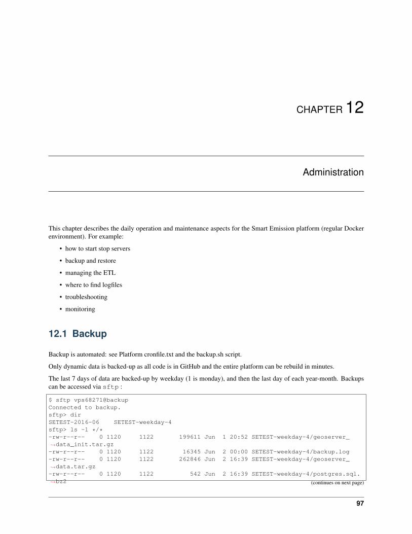
CHAPTER 12
Administration
This chapter describes the daily operation and maintenance aspects for the Smart Emission platform (regular Dockerenvironment). For example:
• how to start stop servers
• backup and restore
• managing the ETL
• where to find logfiles
• troubleshooting
• monitoring
12.1 Backup
Backup is automated: see Platform cronfile.txt and the backup.sh script.
Only dynamic data is backed-up as all code is in GitHub and the entire platform can be rebuild in minutes.
The last 7 days of data are backed-up by weekday (1 is monday), and then the last day of each year-month. Backupscan be accessed via sftp :
$ sftp vps68271@backupConnected to backup.sftp> dirSETEST-2016-06 SETEST-weekday-4sftp> ls -l */*-rw-r--r-- 0 1120 1122 199611 Jun 1 20:52 SETEST-weekday-4/geoserver_→˓data_init.tar.gz-rw-r--r-- 0 1120 1122 16345 Jun 2 00:00 SETEST-weekday-4/backup.log-rw-r--r-- 0 1120 1122 262846 Jun 2 16:39 SETEST-weekday-4/geoserver_→˓data.tar.gz-rw-r--r-- 0 1120 1122 542 Jun 2 16:39 SETEST-weekday-4/postgres.sql.→˓bz2 (continues on next page)
97
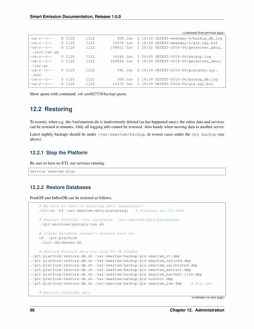
Smart Emission Documentation, Release 1.0.0
(continued from previous page)
-rw-r--r-- 0 1120 1122 308 Jun 2 16:39 SETEST-weekday-4/backup_db.log-rw-r--r-- 0 1120 1122 13570 Jun 2 16:39 SETEST-weekday-4/gis.sql.bz2-rw-r--r-- 0 1120 1122 199611 Jun 1 20:52 SETEST-2016-06/geoserver_data_→˓init.tar.gz-rw-r--r-- 0 1120 1122 16345 Jun 2 00:00 SETEST-2016-06/backup.log-rw-r--r-- 0 1120 1122 262846 Jun 2 16:39 SETEST-2016-06/geoserver_data.→˓tar.gz-rw-r--r-- 0 1120 1122 542 Jun 2 16:39 SETEST-2016-06/postgres.sql.→˓bz2-rw-r--r-- 0 1120 1122 308 Jun 2 16:39 SETEST-2016-06/backup_db.log-rw-r--r-- 0 1120 1122 13570 Jun 2 16:39 SETEST-2016-06/gis.sql.bz2
Show quota with command: ssh vps68271@backup quota.
12.2 Restoring
To restore, when e.g. the /var/smartem dir is inadvertently deleted (as has happened once), the entire data and servicescan be restored in minutes. Only all logging info cannot be restored. Also handy when moving data to another server.
Latest nightly backups should be under /var/smartem/backup, in worser cases under the vps backup (seeabove).
12.2.1 Stop the Platform
Be sure to have no ETL nor services running.
service smartem stop
12.2.2 Restore Databases
PostGIS and InfluxDB can be restored as follows.
# Be sure to have no dangling data (dangerous!)/bin/rm -rf /var/smartem/data/postgresql # contains all PG data
# Restart PostGIS: this recreates /var/smartem/data/postgresql~/git/services/postgis/run.sh
# creeer database schema's globale vars etccd ~/git/platform./init-databases.sh
# Restore PostGIS data for each PG DB schema~/git/platform/restore-db.sh /var/smartem/backup/gis-smartem_rt.dmp~/git/platform/restore-db.sh /var/smartem/backup/gis-smartem_refined.dmp~/git/platform/restore-db.sh /var/smartem/backup/gis-smartem_calibrated.dmp~/git/platform/restore-db.sh /var/smartem/backup/gis-smartem_extract.dmp~/git/platform/restore-db.sh /var/smartem/backup/gis-smartem_harvest-rivm.dmp~/git/platform/restore-db.sh /var/smartem/backup/gis-sos52n1.dmp~/git/platform/restore-db.sh /var/smartem/backup/gis-smartem_raw.dmp # big one
# Restore InfluxDB data(continues on next page)
98 Chapter 12. Administration
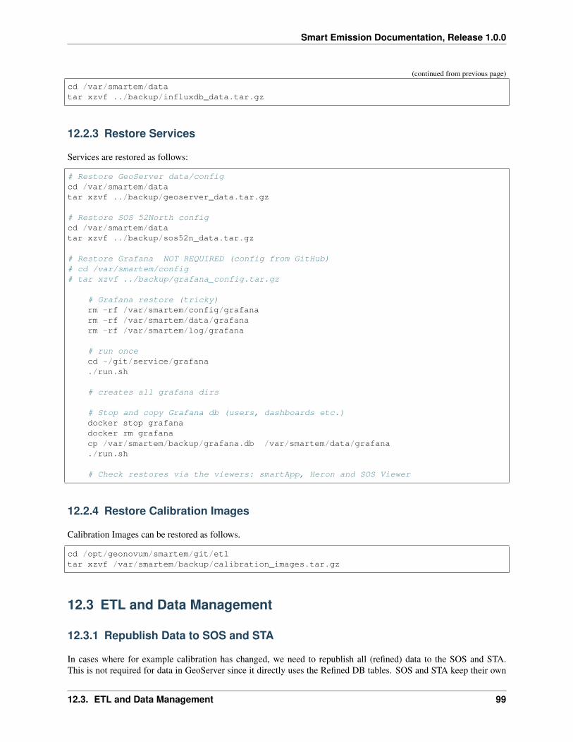
Smart Emission Documentation, Release 1.0.0
(continued from previous page)
cd /var/smartem/datatar xzvf ../backup/influxdb_data.tar.gz
12.2.3 Restore Services
Services are restored as follows:
# Restore GeoServer data/configcd /var/smartem/datatar xzvf ../backup/geoserver_data.tar.gz
# Restore SOS 52North configcd /var/smartem/datatar xzvf ../backup/sos52n_data.tar.gz
# Restore Grafana NOT REQUIRED (config from GitHub)# cd /var/smartem/config# tar xzvf ../backup/grafana_config.tar.gz
# Grafana restore (tricky)rm -rf /var/smartem/config/grafanarm -rf /var/smartem/data/grafanarm -rf /var/smartem/log/grafana
# run oncecd ~/git/service/grafana./run.sh
# creates all grafana dirs
# Stop and copy Grafana db (users, dashboards etc.)docker stop grafanadocker rm grafanacp /var/smartem/backup/grafana.db /var/smartem/data/grafana./run.sh
# Check restores via the viewers: smartApp, Heron and SOS Viewer
12.2.4 Restore Calibration Images
Calibration Images can be restored as follows.
cd /opt/geonovum/smartem/git/etltar xzvf /var/smartem/backup/calibration_images.tar.gz
12.3 ETL and Data Management
12.3.1 Republish Data to SOS and STA
In cases where for example calibration has changed, we need to republish all (refined) data to the SOS and STA.This is not required for data in GeoServer since it directly uses the Refined DB tables. SOS and STA keep their own
12.3. ETL and Data Management 99
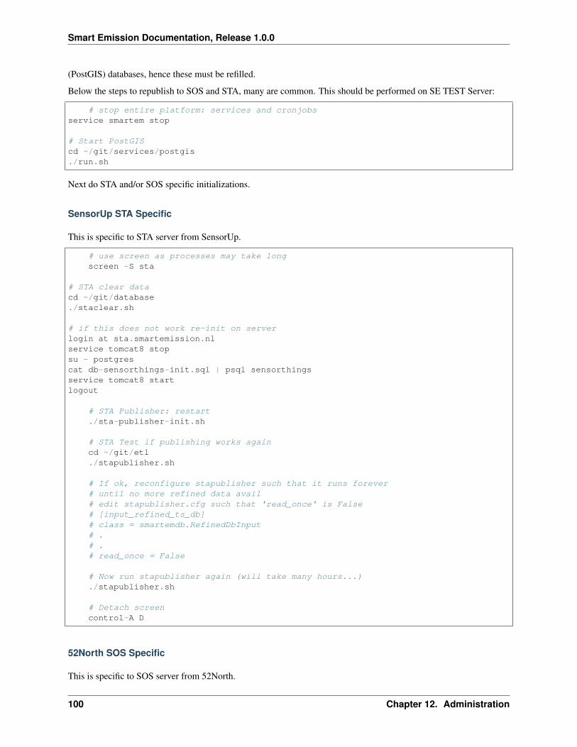
Smart Emission Documentation, Release 1.0.0
(PostGIS) databases, hence these must be refilled.
Below the steps to republish to SOS and STA, many are common. This should be performed on SE TEST Server:
# stop entire platform: services and cronjobsservice smartem stop
# Start PostGIScd ~/git/services/postgis./run.sh
Next do STA and/or SOS specific initializations.
SensorUp STA Specific
This is specific to STA server from SensorUp.
# use screen as processes may take longscreen -S sta
# STA clear datacd ~/git/database./staclear.sh
# if this does not work re-init on serverlogin at sta.smartemission.nlservice tomcat8 stopsu - postgrescat db-sensorthings-init.sql | psql sensorthingsservice tomcat8 startlogout
# STA Publisher: restart./sta-publisher-init.sh
# STA Test if publishing works againcd ~/git/etl./stapublisher.sh
# If ok, reconfigure stapublisher such that it runs forever# until no more refined data avail# edit stapublisher.cfg such that 'read_once' is False# [input_refined_ts_db]# class = smartemdb.RefinedDbInput# .# .# read_once = False
# Now run stapublisher again (will take many hours...)./stapublisher.sh
# Detach screencontrol-A D
52North SOS Specific
This is specific to SOS server from 52North.
100 Chapter 12. Administration

Smart Emission Documentation, Release 1.0.0
# Start SOScd ~/git/services/sos52n./run.sh
# SOS clear DB and other datacd ~/git/services/sos52n/config./sos-clear.sh
# SOS Publisher: restartcd ~/git/database/util
./sos-publisher-init.sh
# SOS Test if publishing works againcd ~/git/etl./sospublisher.sh
# If ok, reconfigure sospublisher such that it runs forever# until no more refined data avail# edit sospublisher.cfg such that 'read_once' is False# [input_refined_ts_db]# class = smartemdb.RefinedDbInput# .# .# read_once = False
# use screen as processes may take longscreen -S sos
# Now run sospublisher again (will take many hours...)./sospublisher.sh
# Detach screencontrol-A D
All dynamic data can be found under /var/smartem/data.
12.3.2 Calibration Model
This needs to be intalled from time to time on the production server. Two parts are incolved: database schema (themodel) and images (the results/stats).
All can be restored as follows, assuming we have the data in some backup.
~/git/platform/restore-db.sh gis-smartem_calibrated.dmpcd /opt/geonovum/smartem/git/etltar xzvf calibration_images.tar.gz
12.4 Admin UI
There is a simple password-protected admin UI for several tasks and inpections. The Admin URL can be found viathe “Links” entry SE Platform website (<data|test>.smartemission.nl).
Via a main screen admin tasks and inpections are selected.
12.4. Admin UI 101
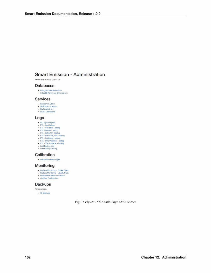
Smart Emission Documentation, Release 1.0.0
Fig. 1: Figure - SE Admin Page Main Screen
102 Chapter 12. Administration

Smart Emission Documentation, Release 1.0.0
12.4.1 Database Management
Management of Postgres/PostGIS DB data is provided via phppgadmin.
Fig. 2: Figure - Postgres DB Management via phppgadmin
Management of InfluxDB data is provided via Chronograf.
Also possibility to develop dashboards.
12.4.2 Services Management
Most of the application servers provide their own management web UI. These can be invoked from the admin page aswell, for example:
• GeoServer Admin
• SOS 52North Admin
• Grafana Admin
• SensorThings API (via GOST) Dashboard
12.4.3 Log Inspection
All log files for the ETL and for the application services can be accessed via the admin screen.
12.4. Admin UI 103
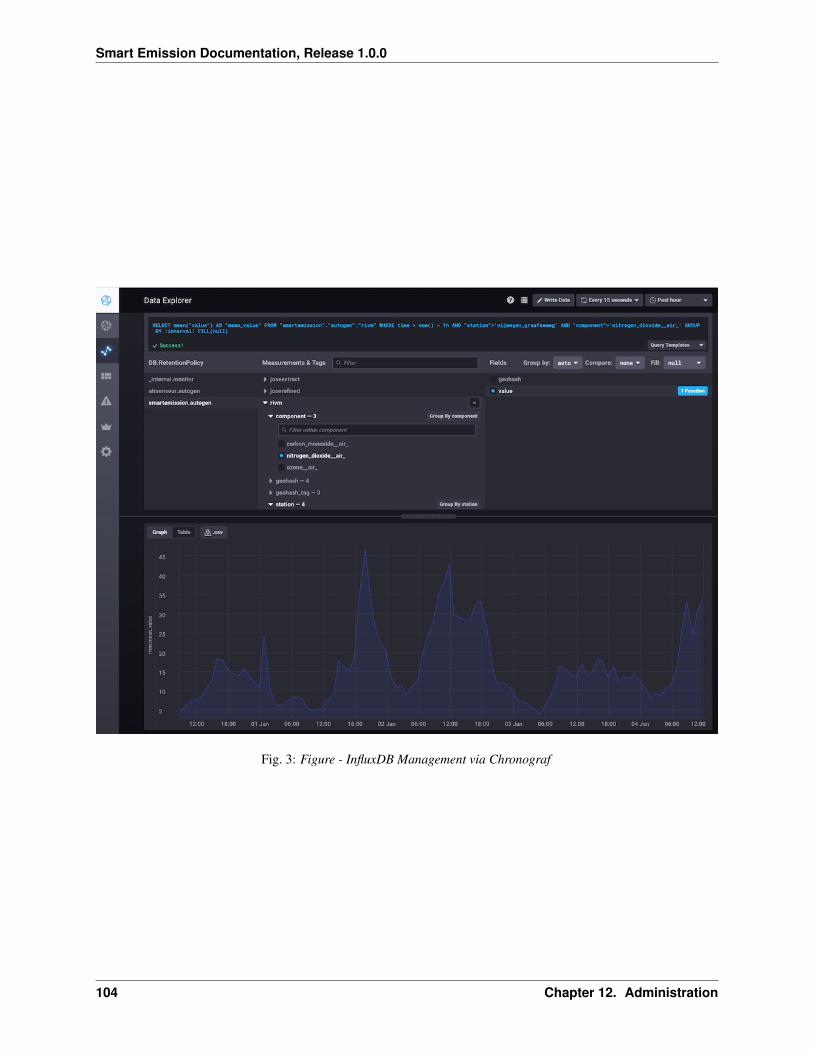
Smart Emission Documentation, Release 1.0.0
Fig. 3: Figure - InfluxDB Management via Chronograf
104 Chapter 12. Administration
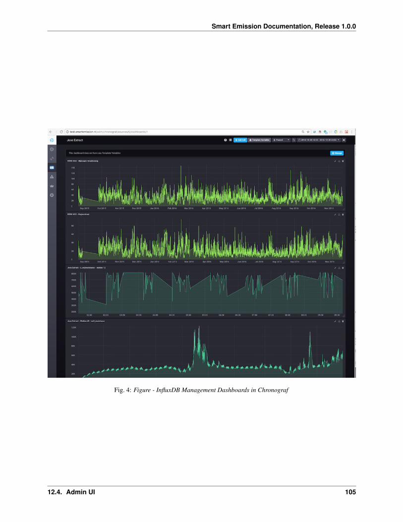
Smart Emission Documentation, Release 1.0.0
Fig. 4: Figure - InfluxDB Management Dashboards in Chronograf
12.4. Admin UI 105
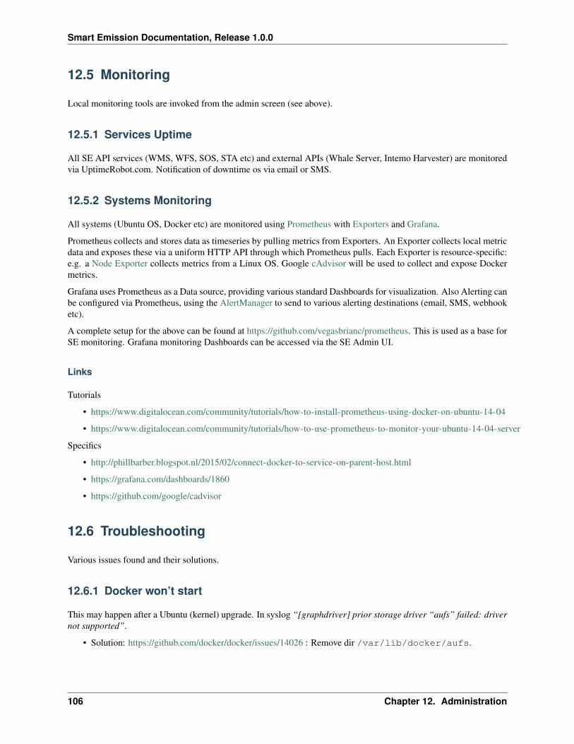
Smart Emission Documentation, Release 1.0.0
12.5 Monitoring
Local monitoring tools are invoked from the admin screen (see above).
12.5.1 Services Uptime
All SE API services (WMS, WFS, SOS, STA etc) and external APIs (Whale Server, Intemo Harvester) are monitoredvia UptimeRobot.com. Notification of downtime os via email or SMS.
12.5.2 Systems Monitoring
All systems (Ubuntu OS, Docker etc) are monitored using Prometheus with Exporters and Grafana.
Prometheus collects and stores data as timeseries by pulling metrics from Exporters. An Exporter collects local metricdata and exposes these via a uniform HTTP API through which Prometheus pulls. Each Exporter is resource-specific:e.g. a Node Exporter collects metrics from a Linux OS. Google cAdvisor will be used to collect and expose Dockermetrics.
Grafana uses Prometheus as a Data source, providing various standard Dashboards for visualization. Also Alerting canbe configured via Prometheus, using the AlertManager to send to various alerting destinations (email, SMS, webhooketc).
A complete setup for the above can be found at https://github.com/vegasbrianc/prometheus. This is used as a base forSE monitoring. Grafana monitoring Dashboards can be accessed via the SE Admin UI.
Links
Tutorials
• https://www.digitalocean.com/community/tutorials/how-to-install-prometheus-using-docker-on-ubuntu-14-04
• https://www.digitalocean.com/community/tutorials/how-to-use-prometheus-to-monitor-your-ubuntu-14-04-server
Specifics
• http://phillbarber.blogspot.nl/2015/02/connect-docker-to-service-on-parent-host.html
• https://grafana.com/dashboards/1860
• https://github.com/google/cadvisor
12.6 Troubleshooting
Various issues found and their solutions.
12.6.1 Docker won’t start
This may happen after a Ubuntu (kernel) upgrade. In syslog “[graphdriver] prior storage driver “aufs” failed: drivernot supported”.
• Solution: https://github.com/docker/docker/issues/14026 : Remove dir /var/lib/docker/aufs.
106 Chapter 12. Administration
Smart Emission Documentation, Release 1.0.0
Fig. 5: Figure - Docker Monitoring in SE
12.6. Troubleshooting 107

Smart Emission Documentation, Release 1.0.0
108 Chapter 12. Administration
CHAPTER 13
Dissemination
This chapter collects various presentations and documents related to dissemination events like workshops and pre-sentations. All “raw” documents can be found in the project GitHub repository at https://github.com/smartemission/smartemission/tree/master/docs/platform/_static/dissemination.
13.1 Workshop 17 dec 2015
In the context of the Smart Emission project a workshop was held at Geonovum on Dec 17, 2015. The main subjectswere:
• presenting OGC standards in general (WMS, WFS, CSW) and in particular Sensor-related (SWE, SOS)
• hands-on demo’s for several clients and visualisations (QGIS, ArcGIS and Heron)
13.1.1 Slides
The agenda and presentation slides, all in PDF, can be found here:
• Workshop Agenda
• OGC Standards+INSPIRE - Thijs Brentjens
• OGC SWE/SOS - Just van den Broecke
• Visualisation in ArcGIS of LML data - Graduation Presentation - Freek Thuis
• QGIS - Matthijs Kastelijns
• Heron Viewer - Just van den Broecke
13.1.2 Links
More detailed tutorials on OGC standards at the OGC School in particular the entire PDF document (18MB!).
109

Smart Emission Documentation, Release 1.0.0
Some interactive visualisation examples “via Google” were also shown like made with D3JS:
• Visualization of Beijing Air Pollution: http://vis.pku.edu.cn/course/Visualization_2012F/assignment2/Chengye
• More can be found here http://vis.pku.edu.cn/wiki/public_course/visclass_f12/assignment/a02/websites/start(click “Alive Version” for each)
13.2 Citizen Meetup 26 may 2016
Meeting held in Nijmegen, on May 26 2016.
13.2.1 Slides
The agenda and presentation slides, all in PDF, can be found here:
• Agenda
• Data, Viewers, Standards - 10 min talk
13.3 Project Meeting 12 july 2016
Meeting held in Nijmegen, on July 12 2016.
• Gas Calibration - Pieter Marsman
13.4 Geospatial World Forum 24 may 2016
Smart Emission was presented at the Geospatial World Forum (GWF) in Rotterdam on may 24, 2016. The presentationfrom Smart Emission is here:
• Smart Emission
13.5 Sensor Webs Conference 30 aug 2016
Smart Emission was presented at the Geospatial Sensor Webs conference organized by 52°North in Münster Germany.
“Under the motto “Geospatial Sensor Webs”, the 52°North Open Innovation Network aims to provide a forum inwhich sensor web researchers and practitioners can present and discuss their ideas, use cases and solutions. . . .The 2016 Workshop and Conference continues the series of 52°North workshops on Sensor Web technologies, whichstarted in 2013.”
13.5.1 Slides
All presentations can be found online at http://52north.org/about/other-activities/geospatial-sensor-webs-conference/program/tuesday
The presentation from Smart Emission is here:
• Smart Emission, building a spatial data infrastructure for an environmental citizen sensor network
110 Chapter 13. Dissemination
Smart Emission Documentation, Release 1.0.0
13.5.2 Papers
For this conference the SE project submitted a paper for the proceedings. The proceedings named “Proceedings ofthe Geospatial Sensor Webs Conference 2016”, Münster, Germany, August 29 - 31, 2016 by Simon Jirka, ChristophStasch, Ann Hitchcock (Eds) can be found online at http://ceur-ws.org/Vol-1762/
The SE-paper “Smart Emission - Building a Spatial Data Infrastructure for an Environmental Citizen Sensor Network”by Michel Grothe et al is here as PDF:
• Smart Emission - Building a Spatial Data Infrastructure for an Environmental Citizen Sensor Network
13.5.3 Links
• Conference web site
13.6 Evaluation Meeting 21 sep 2016
An internal and external evalution meeting was held on sept 21, 2016 in “Wijkcentrum De Biezantijn”, Nijmegen.
13.6.1 Slides
The presentation from Smart Emission is here:
• Status update Data Platform (Just van den Broecke)
• SE Data Platform Overview (Just van den Broecke)
13.7 Presentation 28 nov 2016
An internal presentation on Smart Emission, AirSensEUR and SensorThings API was held on nov 28, 2016 at the“Springplank” lunch meetup at Geonovum.
13.7.1 Slides
The presentation slides are here:
• Smart Emission and more (Just van den Broecke)
13.8 Symposium RIVM “Samen meten aan Luchtkwaliteit”
Op 7 december 2016 organiseerde het RIVM centrum Milieukwaliteit het symposium “Samen meten aan luchtk-waliteit: innovatie, sensoren en citizen science”. Tijdens het symposium kwamen partijen bijeen die de lokale lucht-metingen naar een hoger plan tillen.
SE held a workshop on “Data”. Links below:
• Agenda Symposium
• Aankondiging
13.6. Evaluation Meeting 21 sep 2016 111
Smart Emission Documentation, Release 1.0.0
13.8.1 Slides
The presentation slides (PDF and PPT) from the Smart Emission Data workshop (Verdonk, Nouwens, van denBroecke, Geurts) are here:
• Smart Emission Workshop on Data (PDF)
• Smart Emission Workshop on Data (Powerpoint)
13.9 Presentatie bij RIVM - 17 jan 2017
Presentatie door Just van den Broecke in kader mogelijke overdracht/samenwerking met RIVM voor het SE Platform.
13.9.1 Slides
The presentation slides (PDF) are here:
• Smart Emission Platform (PDF)
13.10 Emit Blog Posts - 2018+
Emit #1+ – series of blog posts on SE Platform by Just van den Broecke on justobjects.nl
13.11 INSPIRE Conference 2018 - Antwerp
Presented by Linda Carton at INSPIRE Conference in Antwerp on sept 20, 2018:
• Title: Development of a national Spatial Data Infrastructure for Open Sensor Data based on citizen scienceinitiatives
• Authors: Linda Carton, Paul Geurts, Just van den Broecke, Janus Hoeks, Michel Grothe, Robert Kieboom,Hester Volten, Jene van der Heide, Marga Jacobs and Piet Biemans
• Abstract
• Presentation Slides (PDF)
13.12 Geo Gebruikersfestival 2018 - Amersfoort
Presented by Just van den Broecke at Geo Gebruikersfestival/SDI.Next 2018 in Amersfoort on okt 31, 2018.
Abstract:
"Eind september heeft PDOK het beheer van het SmartEmissions Platform op zich genomen. Daarmee is deSensordata Stack op PDOK live gegaan. Het PDOK ITteamheeft veel kennis kunnen opdoen over sensordatastromen,onder andere door de inzet van de OGCSensorThingsAPI. Just van den Broecke was zowel bij deopzet van het Smart Emissions Platform zelf betrokken
(continues on next page)
112 Chapter 13. Dissemination
Smart Emission Documentation, Release 1.0.0
(continued from previous page)
als bij de landing hiervan in PDOK. Hij vertelt over degekozen architectuur en standaarden en werpt alvasteen blik in de toekomst."
• Title: SensorSDI op PDOK met het Smart Emission Data Platform
• Author: Just van den Broecke
• Presentation Slides (PDF)
13.12. Geo Gebruikersfestival 2018 - Amersfoort 113
Smart Emission Documentation, Release 1.0.0
114 Chapter 13. Dissemination
CHAPTER 14
Cookbook
This chapter contains sections to aid developers to interact with the SE platform. This is split into the following areas:
• developing (web) clients that use the OGC web services (WFS, WMS, SOS, STA)
• developing new sensor types
• deploying subsets of the SE platform
14.1 Developing Web Clients
The SE platform supports various standard OGC web APIs:
• WMS with Time Dimensions
• WFS
• Sensor Observation Service (SOS)
• SensorThings API (STA)
The use of STA is favoured over SOS.
14.2 SensorThings API
The easiest way to get data out of the SE Platform is via the SensorThings API. As this API is REST-based one canalready navigate through its entities via a web browser. For example the URL http://data.smartemission.nl/gost/v1.0will show all Entities. Each can be clicked to navigate through the model.
14.2.1 Resources
Some STA documentation, inparticular API usage.
115
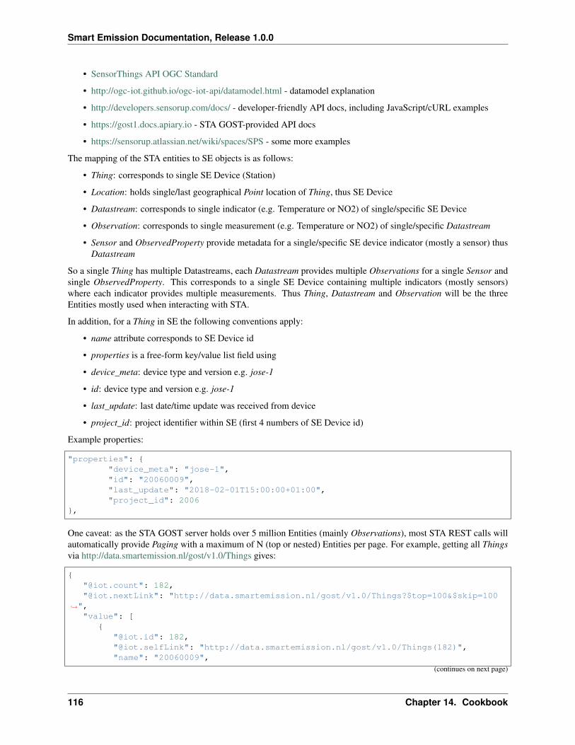
Smart Emission Documentation, Release 1.0.0
• SensorThings API OGC Standard
• http://ogc-iot.github.io/ogc-iot-api/datamodel.html - datamodel explanation
• http://developers.sensorup.com/docs/ - developer-friendly API docs, including JavaScript/cURL examples
• https://gost1.docs.apiary.io - STA GOST-provided API docs
• https://sensorup.atlassian.net/wiki/spaces/SPS - some more examples
The mapping of the STA entities to SE objects is as follows:
• Thing: corresponds to single SE Device (Station)
• Location: holds single/last geographical Point location of Thing, thus SE Device
• Datastream: corresponds to single indicator (e.g. Temperature or NO2) of single/specific SE Device
• Observation: corresponds to single measurement (e.g. Temperature or NO2) of single/specific Datastream
• Sensor and ObservedProperty provide metadata for a single/specific SE device indicator (mostly a sensor) thusDatastream
So a single Thing has multiple Datastreams, each Datastream provides multiple Observations for a single Sensor andsingle ObservedProperty. This corresponds to a single SE Device containing multiple indicators (mostly sensors)where each indicator provides multiple measurements. Thus Thing, Datastream and Observation will be the threeEntities mostly used when interacting with STA.
In addition, for a Thing in SE the following conventions apply:
• name attribute corresponds to SE Device id
• properties is a free-form key/value list field using
• device_meta: device type and version e.g. jose-1
• id: device type and version e.g. jose-1
• last_update: last date/time update was received from device
• project_id: project identifier within SE (first 4 numbers of SE Device id)
Example properties:
"properties": {"device_meta": "jose-1","id": "20060009","last_update": "2018-02-01T15:00:00+01:00","project_id": 2006
},
One caveat: as the STA GOST server holds over 5 million Entities (mainly Observations), most STA REST calls willautomatically provide Paging with a maximum of N (top or nested) Entities per page. For example, getting all Thingsvia http://data.smartemission.nl/gost/v1.0/Things gives:
{"@iot.count": 182,"@iot.nextLink": "http://data.smartemission.nl/gost/v1.0/Things?$top=100&$skip=100
→˓","value": [
{"@iot.id": 182,"@iot.selfLink": "http://data.smartemission.nl/gost/v1.0/Things(182)","name": "20060009",
(continues on next page)
116 Chapter 14. Cookbook
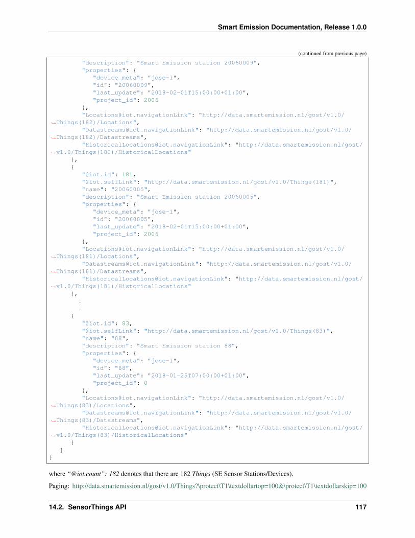
Smart Emission Documentation, Release 1.0.0
(continued from previous page)
"description": "Smart Emission station 20060009","properties": {
"device_meta": "jose-1","id": "20060009","last_update": "2018-02-01T15:00:00+01:00","project_id": 2006
},"[email protected]": "http://data.smartemission.nl/gost/v1.0/
→˓Things(182)/Locations","[email protected]": "http://data.smartemission.nl/gost/v1.0/
→˓Things(182)/Datastreams","[email protected]": "http://data.smartemission.nl/gost/
→˓v1.0/Things(182)/HistoricalLocations"},{
"@iot.id": 181,"@iot.selfLink": "http://data.smartemission.nl/gost/v1.0/Things(181)","name": "20060005","description": "Smart Emission station 20060005","properties": {
"device_meta": "jose-1","id": "20060005","last_update": "2018-02-01T15:00:00+01:00","project_id": 2006
},"[email protected]": "http://data.smartemission.nl/gost/v1.0/
→˓Things(181)/Locations","[email protected]": "http://data.smartemission.nl/gost/v1.0/
→˓Things(181)/Datastreams","[email protected]": "http://data.smartemission.nl/gost/
→˓v1.0/Things(181)/HistoricalLocations"},
.
.{
"@iot.id": 83,"@iot.selfLink": "http://data.smartemission.nl/gost/v1.0/Things(83)","name": "88","description": "Smart Emission station 88","properties": {
"device_meta": "jose-1","id": "88","last_update": "2018-01-25T07:00:00+01:00","project_id": 0
},"[email protected]": "http://data.smartemission.nl/gost/v1.0/
→˓Things(83)/Locations","[email protected]": "http://data.smartemission.nl/gost/v1.0/
→˓Things(83)/Datastreams","[email protected]": "http://data.smartemission.nl/gost/
→˓v1.0/Things(83)/HistoricalLocations"}
]}
where “@iot.count”: 182 denotes that there are 182 Things (SE Sensor Stations/Devices).
Paging: http://data.smartemission.nl/gost/v1.0/Things?\protect\T1\textdollartop=100&\protect\T1\textdollarskip=100
14.2. SensorThings API 117
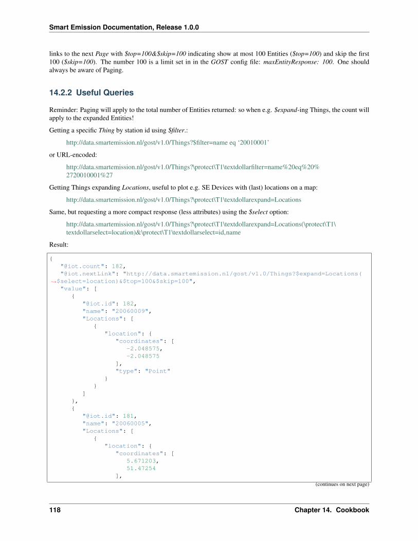
Smart Emission Documentation, Release 1.0.0
links to the next Page with $top=100&$skip=100 indicating show at most 100 Entities ($top=100) and skip the first100 ($skip=100). The number 100 is a limit set in in the GOST config file: maxEntityResponse: 100. One shouldalways be aware of Paging.
14.2.2 Useful Queries
Reminder: Paging will apply to the total number of Entities returned: so when e.g. $expand-ing Things, the count willapply to the expanded Entities!
Getting a specific Thing by station id using $filter.:
http://data.smartemission.nl/gost/v1.0/Things?$filter=name eq ‘20010001’
or URL-encoded:
http://data.smartemission.nl/gost/v1.0/Things?\protect\T1\textdollarfilter=name%20eq%20%2720010001%27
Getting Things expanding Locations, useful to plot e.g. SE Devices with (last) locations on a map:
http://data.smartemission.nl/gost/v1.0/Things?\protect\T1\textdollarexpand=Locations
Same, but requesting a more compact response (less attributes) using the $select option:
http://data.smartemission.nl/gost/v1.0/Things?\protect\T1\textdollarexpand=Locations(\protect\T1\textdollarselect=location)&\protect\T1\textdollarselect=id,name
Result:
{"@iot.count": 182,"@iot.nextLink": "http://data.smartemission.nl/gost/v1.0/Things?$expand=Locations(
→˓$select=location)&$top=100&$skip=100","value": [
{"@iot.id": 182,"name": "20060009","Locations": [
{"location": {
"coordinates": [-2.048575,-2.048575
],"type": "Point"
}}
]},{
"@iot.id": 181,"name": "20060005","Locations": [
{"location": {
"coordinates": [5.671203,51.47254
],
(continues on next page)
118 Chapter 14. Cookbook
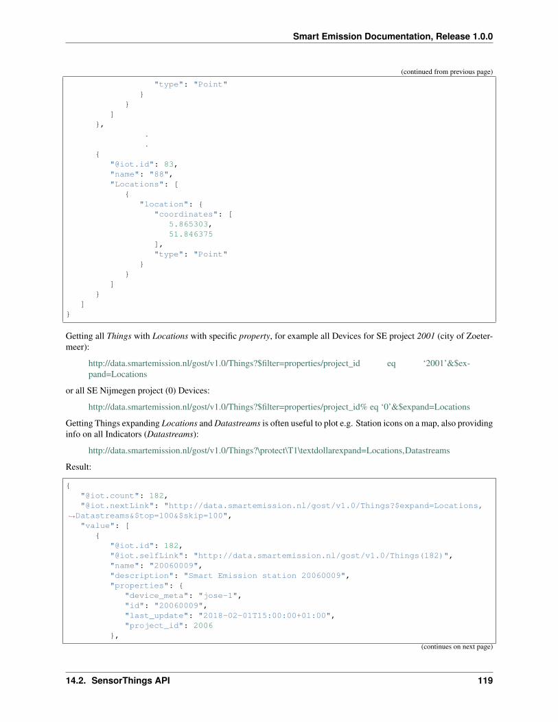
Smart Emission Documentation, Release 1.0.0
(continued from previous page)
"type": "Point"}
}]
},..
{"@iot.id": 83,"name": "88","Locations": [
{"location": {
"coordinates": [5.865303,51.846375
],"type": "Point"
}}
]}
]}
Getting all Things with Locations with specific property, for example all Devices for SE project 2001 (city of Zoeter-meer):
http://data.smartemission.nl/gost/v1.0/Things?$filter=properties/project_id eq ‘2001’&$ex-pand=Locations
or all SE Nijmegen project (0) Devices:
http://data.smartemission.nl/gost/v1.0/Things?$filter=properties/project_id% eq ‘0’&$expand=Locations
Getting Things expanding Locations and Datastreams is often useful to plot e.g. Station icons on a map, also providinginfo on all Indicators (Datastreams):
http://data.smartemission.nl/gost/v1.0/Things?\protect\T1\textdollarexpand=Locations,Datastreams
Result:
{"@iot.count": 182,"@iot.nextLink": "http://data.smartemission.nl/gost/v1.0/Things?$expand=Locations,
→˓Datastreams&$top=100&$skip=100","value": [
{"@iot.id": 182,"@iot.selfLink": "http://data.smartemission.nl/gost/v1.0/Things(182)","name": "20060009","description": "Smart Emission station 20060009","properties": {
"device_meta": "jose-1","id": "20060009","last_update": "2018-02-01T15:00:00+01:00","project_id": 2006
},
(continues on next page)
14.2. SensorThings API 119

Smart Emission Documentation, Release 1.0.0
(continued from previous page)
"[email protected]": "http://data.smartemission.nl/gost/→˓v1.0/Things(182)/HistoricalLocations",
"Locations": [{
"@iot.id": 182,"@iot.selfLink": "http://data.smartemission.nl/gost/v1.0/Locations(182)
→˓","name": "20060009","description": "Location of Station 20060009","encodingType": "application/vnd.geo+json","location": {
"coordinates": [-2.048575,-2.048575
],"type": "Point"
},"[email protected]": "http://data.smartemission.nl/gost/v1.0/
→˓Locations(182)/Things","[email protected]": "http://data.smartemission.
→˓nl/gost/v1.0/Locations(182)/HistoricalLocations"}
],"Datastreams": [
{"@iot.id": 1690,"@iot.selfLink": "http://data.smartemission.nl/gost/v1.0/
→˓Datastreams(1690)","name": "pm2_5","description": "PM 2.5 for Station 20060009","unitOfMeasurement": {
"definition": "http://unitsofmeasure.org/ucum.html#para-30","name": "PM 2.5","symbol": "ug/m3"
},"observationType": "http://www.opengis.net/def/observationType/OGC-OM/
→˓2.0/OM_Measurement","[email protected]": "http://data.smartemission.nl/gost/v1.0/
→˓Datastreams(1690)/Thing","[email protected]": "http://data.smartemission.nl/gost/v1.0/
→˓Datastreams(1690)/Sensor","[email protected]": "http://data.smartemission.nl/gost/
→˓v1.0/Datastreams(1690)/Observations","[email protected]": "http://data.smartemission.nl/
→˓gost/v1.0/Datastreams(1690)/ObservedProperty"},{
"@iot.id": 1689,"@iot.selfLink": "http://data.smartemission.nl/gost/v1.0/
→˓Datastreams(1689)","name": "pm10","description": "PM 10 for Station 20060009","unitOfMeasurement": {
"definition": "http://unitsofmeasure.org/ucum.html#para-30","name": "PM 10","symbol": "ug/m3"
},(continues on next page)
120 Chapter 14. Cookbook

Smart Emission Documentation, Release 1.0.0
(continued from previous page)
"observationType": "http://www.opengis.net/def/observationType/OGC-OM/→˓2.0/OM_Measurement",
"[email protected]": "http://data.smartemission.nl/gost/v1.0/→˓Datastreams(1689)/Thing",
"[email protected]": "http://data.smartemission.nl/gost/v1.0/→˓Datastreams(1689)/Sensor",
"[email protected]": "http://data.smartemission.nl/gost/→˓v1.0/Datastreams(1689)/Observations",
"[email protected]": "http://data.smartemission.nl/→˓gost/v1.0/Datastreams(1689)/ObservedProperty"
},
Getting specific Datastreams for single Indicator, for example getting all NO2 Datastreams.
http://data.smartemission.nl/gost/v1.0/Datastreams?$filter=name eq ‘no2’
Getting Observations
Getting last Observations since date/time:
http://data.smartemission.nl/gost/v1.0/Observations?$filter=phenomenonTime gt ‘2018-02-06T08:00:00.000Z’
Result:
{"@iot.count": 921,"@iot.nextLink": "http://data.smartemission.nl/gost/v1.0/Observations?
→˓$filter=phenomenonTime gt '2018-02-06T08:00:00.000Z'&$top=100&$skip=100","value": [
{"@iot.id": 5131983,"@iot.selfLink": "http://data.smartemission.nl/gost/v1.0/
→˓Observations(5131983)","phenomenonTime": "2018-02-06T10:00:00.000Z","result": 1,"parameters": {
"device_meta": "jose-1","gid": 5132008,"name": "noiselevelavg","raw_gid": 492353,"sensor_meta": "au-V30_V3F","station": 20000001
},"[email protected]": "http://data.smartemission.nl/gost/v1.0/
→˓Observations(5131983)/Datastream","[email protected]": "http://data.smartemission.nl/gost/
→˓v1.0/Observations(5131983)/FeatureOfInterest","resultTime": "2018-02-06T11:00:00+01:00"
},{
"@iot.id": 5131982,"@iot.selfLink": "http://data.smartemission.nl/gost/v1.0/
→˓Observations(5131982)","phenomenonTime": "2018-02-06T10:00:00.000Z","result": 1017,"parameters": {
"device_meta": "jose-1",
(continues on next page)
14.2. SensorThings API 121
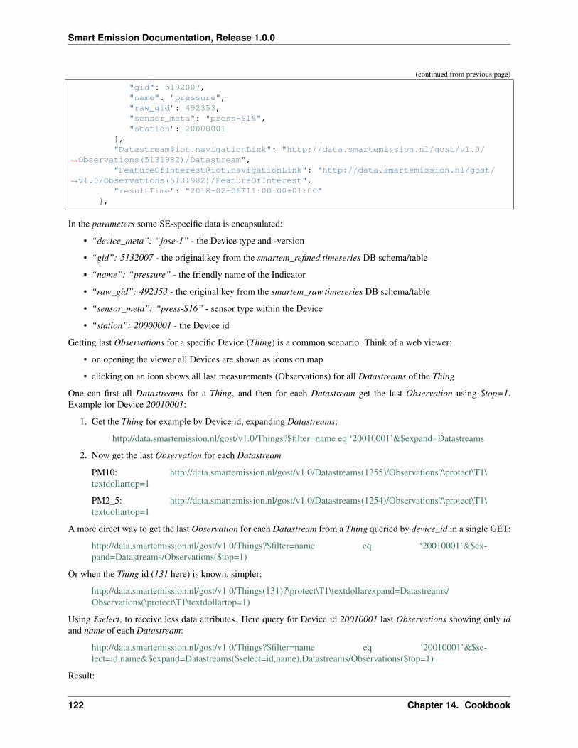
Smart Emission Documentation, Release 1.0.0
(continued from previous page)
"gid": 5132007,"name": "pressure","raw_gid": 492353,"sensor_meta": "press-S16","station": 20000001
},"[email protected]": "http://data.smartemission.nl/gost/v1.0/
→˓Observations(5131982)/Datastream","[email protected]": "http://data.smartemission.nl/gost/
→˓v1.0/Observations(5131982)/FeatureOfInterest","resultTime": "2018-02-06T11:00:00+01:00"
},
In the parameters some SE-specific data is encapsulated:
• “device_meta”: “jose-1” - the Device type and -version
• “gid”: 5132007 - the original key from the smartem_refined.timeseries DB schema/table
• “name”: “pressure” - the friendly name of the Indicator
• “raw_gid”: 492353 - the original key from the smartem_raw.timeseries DB schema/table
• “sensor_meta”: “press-S16” - sensor type within the Device
• “station”: 20000001 - the Device id
Getting last Observations for a specific Device (Thing) is a common scenario. Think of a web viewer:
• on opening the viewer all Devices are shown as icons on map
• clicking on an icon shows all last measurements (Observations) for all Datastreams of the Thing
One can first all Datastreams for a Thing, and then for each Datastream get the last Observation using $top=1.Example for Device 20010001:
1. Get the Thing for example by Device id, expanding Datastreams:
http://data.smartemission.nl/gost/v1.0/Things?$filter=name eq ‘20010001’&$expand=Datastreams
2. Now get the last Observation for each Datastream
PM10: http://data.smartemission.nl/gost/v1.0/Datastreams(1255)/Observations?\protect\T1\textdollartop=1
PM2_5: http://data.smartemission.nl/gost/v1.0/Datastreams(1254)/Observations?\protect\T1\textdollartop=1
A more direct way to get the last Observation for each Datastream from a Thing queried by device_id in a single GET:
http://data.smartemission.nl/gost/v1.0/Things?$filter=name eq ‘20010001’&$ex-pand=Datastreams/Observations($top=1)
Or when the Thing id (131 here) is known, simpler:
http://data.smartemission.nl/gost/v1.0/Things(131)?\protect\T1\textdollarexpand=Datastreams/Observations(\protect\T1\textdollartop=1)
Using $select, to receive less data attributes. Here query for Device id 20010001 last Observations showing only idand name of each Datastream:
http://data.smartemission.nl/gost/v1.0/Things?$filter=name eq ‘20010001’&$se-lect=id,name&$expand=Datastreams($select=id,name),Datastreams/Observations($top=1)
Result:
122 Chapter 14. Cookbook
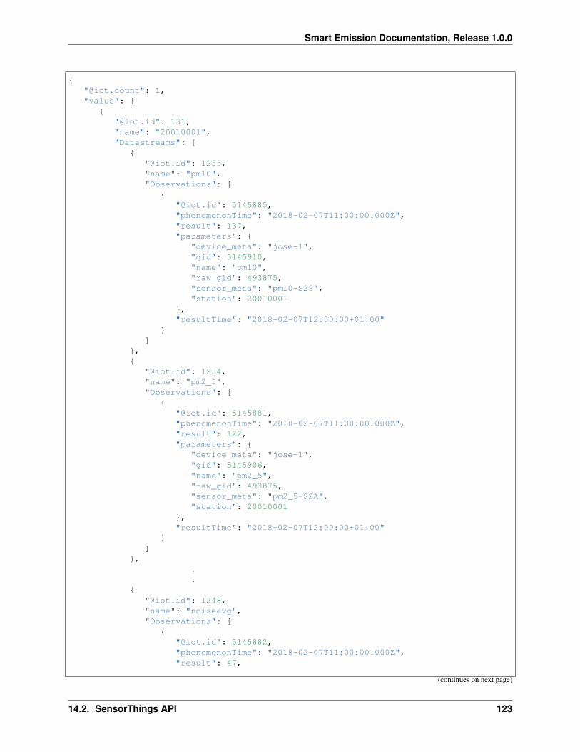
Smart Emission Documentation, Release 1.0.0
{"@iot.count": 1,"value": [
{"@iot.id": 131,"name": "20010001","Datastreams": [
{"@iot.id": 1255,"name": "pm10","Observations": [
{"@iot.id": 5145885,"phenomenonTime": "2018-02-07T11:00:00.000Z","result": 137,"parameters": {
"device_meta": "jose-1","gid": 5145910,"name": "pm10","raw_gid": 493875,"sensor_meta": "pm10-S29","station": 20010001
},"resultTime": "2018-02-07T12:00:00+01:00"
}]
},{
"@iot.id": 1254,"name": "pm2_5","Observations": [
{"@iot.id": 5145881,"phenomenonTime": "2018-02-07T11:00:00.000Z","result": 122,"parameters": {
"device_meta": "jose-1","gid": 5145906,"name": "pm2_5","raw_gid": 493875,"sensor_meta": "pm2_5-S2A","station": 20010001
},"resultTime": "2018-02-07T12:00:00+01:00"
}]
},..
{"@iot.id": 1248,"name": "noiseavg","Observations": [
{"@iot.id": 5145882,"phenomenonTime": "2018-02-07T11:00:00.000Z","result": 47,
(continues on next page)
14.2. SensorThings API 123

Smart Emission Documentation, Release 1.0.0
(continued from previous page)
"parameters": {"device_meta": "jose-1","gid": 5145907,"name": "noiseavg","raw_gid": 493875,"sensor_meta": "au-V30_V3F","station": 20010001
},"resultTime": "2018-02-07T12:00:00+01:00"
}]
}]
}]
}
Last 100 Observations from any Indicators from any Devices:
http://data.smartemission.nl/gost/v1.0/Observations?\protect\T1\textdollartop=100
Result:
{"@iot.count": 5131983,"@iot.nextLink": "http://data.smartemission.nl/gost/v1.0/Observations?$top=100&
→˓$skip=100","value": [
{"@iot.id": 5131983,"@iot.selfLink": "http://data.smartemission.nl/gost/v1.0/
→˓Observations(5131983)","phenomenonTime": "2018-02-06T10:00:00.000Z","result": 1,"parameters": {
"device_meta": "jose-1","gid": 5132008,"name": "noiselevelavg","raw_gid": 492353,"sensor_meta": "au-V30_V3F","station": 20000001
},"[email protected]": "http://data.smartemission.nl/gost/v1.0/
→˓Observations(5131983)/Datastream","[email protected]": "http://data.smartemission.nl/gost/
→˓v1.0/Observations(5131983)/FeatureOfInterest","resultTime": "2018-02-06T11:00:00+01:00"
},{
"@iot.id": 5131982,"@iot.selfLink": "http://data.smartemission.nl/gost/v1.0/
→˓Observations(5131982)","phenomenonTime": "2018-02-06T10:00:00.000Z","result": 1017,"parameters": {
"device_meta": "jose-1","gid": 5132007,
(continues on next page)
124 Chapter 14. Cookbook
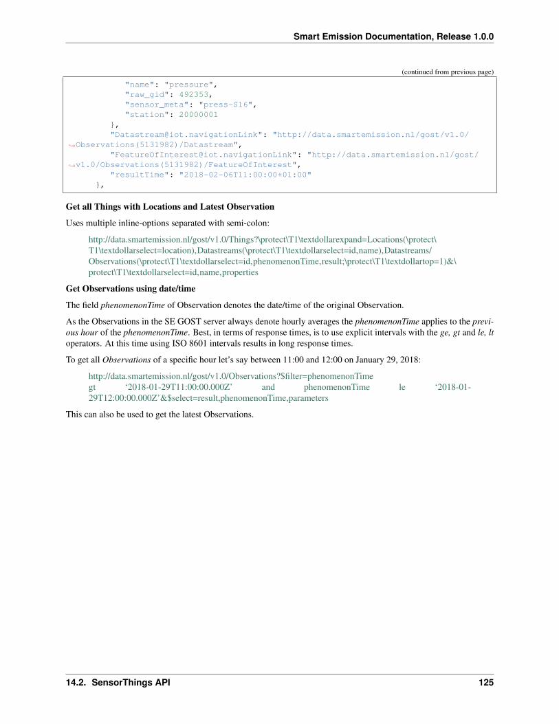
Smart Emission Documentation, Release 1.0.0
(continued from previous page)
"name": "pressure","raw_gid": 492353,"sensor_meta": "press-S16","station": 20000001
},"[email protected]": "http://data.smartemission.nl/gost/v1.0/
→˓Observations(5131982)/Datastream","[email protected]": "http://data.smartemission.nl/gost/
→˓v1.0/Observations(5131982)/FeatureOfInterest","resultTime": "2018-02-06T11:00:00+01:00"
},
Get all Things with Locations and Latest Observation
Uses multiple inline-options separated with semi-colon:
http://data.smartemission.nl/gost/v1.0/Things?\protect\T1\textdollarexpand=Locations(\protect\T1\textdollarselect=location),Datastreams(\protect\T1\textdollarselect=id,name),Datastreams/Observations(\protect\T1\textdollarselect=id,phenomenonTime,result;\protect\T1\textdollartop=1)&\protect\T1\textdollarselect=id,name,properties
Get Observations using date/time
The field phenomenonTime of Observation denotes the date/time of the original Observation.
As the Observations in the SE GOST server always denote hourly averages the phenomenonTime applies to the previ-ous hour of the phenomenonTime. Best, in terms of response times, is to use explicit intervals with the ge, gt and le, ltoperators. At this time using ISO 8601 intervals results in long response times.
To get all Observations of a specific hour let’s say between 11:00 and 12:00 on January 29, 2018:
http://data.smartemission.nl/gost/v1.0/Observations?$filter=phenomenonTimegt ‘2018-01-29T11:00:00.000Z’ and phenomenonTime le ‘2018-01-29T12:00:00.000Z’&$select=result,phenomenonTime,parameters
This can also be used to get the latest Observations.
14.2. SensorThings API 125

Smart Emission Documentation, Release 1.0.0
126 Chapter 14. Cookbook
CHAPTER 15
Evolution
By: Just van den Broecke - v1 - March 2, 2018 - written @Kadaster/PDOK.
This is a chapter from the full Smart Emission platform documentation found at http://smartplatform.readthedocs.io
This chapter focuses on possible future evolution scenarios for the Smart Emission platform.
See the Architecture, Data Management, Components and Dataflow and APIs chapters for the overall design and dataprocessing, APIs and dataflow of the SE Platform.
15.1 Introduction
Within the world of SensorWeb and IoT, many platforms are developed and offered. Some with Open Source, otherswith proprietary source. Data may be Open, partially Open or completely closed. Same goes for standards and APIsused for (web) services. Some platforms are “end-to-end complete”: they include data acquisition from sensors,data management/storage, services and viewers, often in the form of a “Portal” and “Dashboards”. Most of theseportals are built with proprietary source, use custom APIs and usually provide subscription models (“Cloud Services”)for end users. Also data is usually hosted at major providers like Amazon and Google, most often not within TheNetherlands. Licensing models may change at will. But the convenience is great, often plug-and-play integrations(like with ThingsNetwork). Examples are numerous, we mention just MyDevices Cayenne and OpenSensors.
This chapter is not to list and review all major sensor/IoT platforms, but puts focus on a a very high level functionalarchitecture applied to sensor network initiatives within The Netherlands.
15.2 Components
This section sketches a global and distributed component architecture. From several sensor network projects, includingSmart Emission, and discussions a high-level, global architecture emerged of functional building blocks connected viaAPIs (Standards). This is sketched in Figure 1 below.
Figure 1 above uses three drawing elements:
• the green rectangles denote functional blocks
127
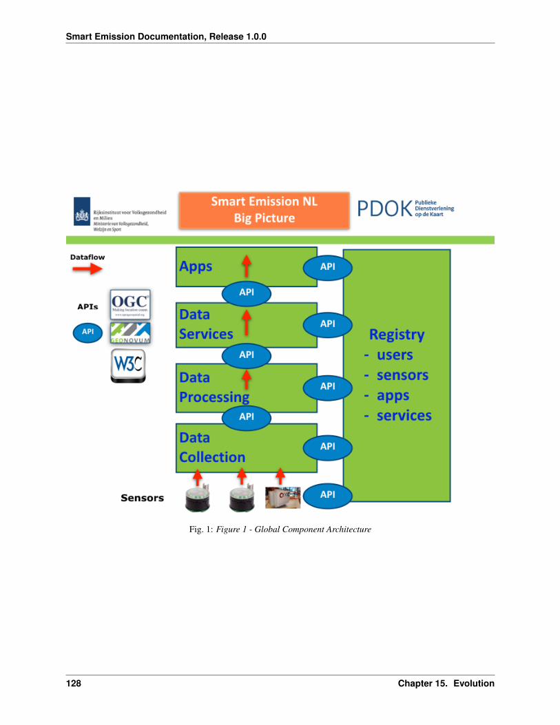
Smart Emission Documentation, Release 1.0.0
Fig. 1: Figure 1 - Global Component Architecture
128 Chapter 15. Evolution
Smart Emission Documentation, Release 1.0.0
• the red arrows denote the flow of sensor data
• the oval elements called “API” denote standardized interaction between functional blocks
Furthermore:
• functional blocks may be distributed over servers (or in same server)
• relations between these blocks may be multiple (many-to-many)
• functional blocks may be provided and maintained by different organizations/companies
The image sketches an architecture on the basis of minimal Coupling and maximum Cohesion: blocks have minimal(API) couplings and are maximally cohesive, i.e. perform only specific tasks.
What follows is a short description of the functions of each block and its relations to other blocks, starting at thebottom, following the flow of (sensor) data.
15.2.1 Data Collection
This block in practice provides one or more Data Collectors. Sensors need to send their data to “somewhere”. Often itis good practice to have a “buffer”, here called a Data Collector that initially receives and stores the data from sensorsand makes it available via an API.
Examples: within the SE Platform, raw data from Josene sensors is sent using low-level protocols (MQTT) to DataCollectors provided by Intemo and CityGIS. These provide storage and the “Whale API” from which any other plat-form SE or RIVM can obtain, i.e. harvest that raw sensor-data.
Another Data Collector within the SE platform is an InfluxDB timeseries database to which for example the EU JRCAirSensEUR stations send their raw sensor data.
The big advantage of this approach is that:
• sensors only need to know a single destination (address) for their data
• there may be multiple raw data consumers (e.g. SE, RIVM) or OTAP streets
• history function: data may be collected and stored for longer periods
The result of this block is that raw sensor-data (timeseries) is stored and made available to multiple consumers. Butthe data is still “raw”, not yet suitable for applications.
NB in addition it is convenient that a Data Collector API always provides a “current/last” dataset from all sensors todata consumers, to allow near-realtime datastreams.
15.2.2 Data Processing
Sensor data provided by Data Collectors is consumed, usually via harvesting by Data Processors. These provide ingeneral the following refinement steps on the raw sensor data:
• validation: removing “outliers”, bad data in general
• conversion: convert units, e.g. from Kelvin to Celsius for temperature
• calibration: provide calibration, e.g. via linear methods, Artificial Neural Networks (ANN)
• aggregation: make averages like hour or 5 minute-values, data reduction
Not all Data Processors will provide all these functions, and implementations may greatly differ.
In the end each Data Processor will make its “refined” data available for the next step: Data Services.
15.2. Components 129
Smart Emission Documentation, Release 1.0.0
15.2.3 Data Services
A Data Service in general provides usually a Web API through which consumers, mainly Applications can utilize therefined sensor-data by the Data Processors.
In this block Web Service APIs are found: when standardized these are often OGC-based like the Sensor ObservationService, the SensorThings API (STA), but also WMS and WFS.
For example the SE platform provides currently (feb 2018) five APIs: WMS (Time), WFS, SOS, STA and a properi-etary REST API for current sensor-values. For SOS and STA Data Publishers are defined that push data from DataProcessors to these respective services (via SOS-T and STA REST PUT).
15.2.4 Apps
Apps are web-based, desktop or mobile applications that consume refined sensor-data provided via the (standardized)APIs of the Data Services.
For example within the SE project several “Viewers” were developed. Some internal within the project like the heronand SmartApp, some external like viewers from Imagem and TNO.
15.2.5 Registry
This building block is global to all the other building blocks discussed above. Its functions may be distributed overseveral actual components and may include:
• sensor registration: location, owner etc
• sensor metadata, the properties of the sensor
• user registration: sensor ownership, access constraints
• service registration: available services, service URLs etc
• apps registration: as for services:
This block mainly deals with data and APIs “other than the sensor-data (and APIs)”. Often this is refered to asMetadata (MD) and MD APIs.
This block is often overlooked in projects. At least within the SE Platform it has not been explicitly defined as initiallythere was just one sensor/device type and no users registered. But like in other geospatial architectures this aspectshould be taken into account.
15.3 APIs and Standards
The success of the above architecture has a prominent role for APIs. Especially when building blocks are developedand deployed in a distributed fashion by different organizations.
A few recommendations based on experience within the SE project.
15.3.1 SensorThings API (STA)
The SensorThings API is a relatively new OGC standard. It provides similar functions as SOS, but more “modern”and lightweight.
In a nutshell: within STA an E/R-ike model of Entities (Things, Sensors, Datastreams, Observations etc) are managedvia HTTP verbs (like GET, PUT, PATCH etc).
130 Chapter 15. Evolution

Smart Emission Documentation, Release 1.0.0
The OGC STA standard also uses and integrates the IoT protocol MQTT.
Usage: STA could be applied for several APIs within the above architecture:
• Sensors to Data Collectors (using MQTT)
• Data Services to Apps
15.3.2 Whale API a.k.a. Raw Sensor API
Via this API the SE Harvesters pulled in data from Data Collectors. This custom Web API was developed (by RobertKieboom and Just van den Broecke) specifically for the SE project. It proved very convenient to harvest bulk time-series raw sensor-data.
The Whale API has two main services:
• fetch timeseries (history) data
• fetch latest data of any device (“last” values)
The specification and examples can be found in GitHub: https://github.com/smartemission/smartemission/tree/master/docs/specs/rawsensor-api.
15.3.3 Sensor Observation Service (SOS)
After several years of experience, we don’t recommend using SOS:
• bulky data (XML)
• hard to understand by developers
• hard to manage via SOS-T (e.g. moving sensors)
• only two mature Open Source implementation
• interworking problems (see QGIS SOS plugins)
Though some providers have developed a “SOS-REST” API with JSON data formats these are product-specific andthus proprietary.
Though SensorThings API is very recent and implementations may need to mature, for the future STA seems a betteroption.
15.3.4 Web Map Service (WMS)
A WMS with plain image and time-dimension support. This allows clients to fetch images through history (e.g. witha timeslider in a web-viewer). The WMS OGC Standard provide Dimension-support, in this case time as dimension.
15.3.5 Web Feature Service (WFS)
This allows downloading of timeseries data with geospatial filter-support.
Though WFS could be replaced functionally by SensorThings API.
All in all: what is important is to:
• recognize which APIs are required
• which existing APIs (standards) to choose
15.3. APIs and Standards 131
Smart Emission Documentation, Release 1.0.0
• filling in options in these standards (profiling)
• provide Open Source examples/implementations
15.4 Federated Architecture
The above architecure could be implemented by multiple organizations. For example on the (Dutch) national levelscenarios can be envisioned where local and governmental organizations and parties “from the market” each fill-infunctional blocks based on their specialization. This could result in what could be called a Federated Architecture,i.e. no single party provides/controls all building blocks. In theory any party could join (via the APIs and Registry).
A good example of such a federated architecture brought to practice is The ThingsNetwork (TTN), a community-driven LoRaWAN network based on well-defined components and APIs. Setup for different purpose and domain butworking very well in practice because of well-defined building blocks and APIs, making it extensible as any party canjoin and add a building block. A Forum with community managers and a central website with documentation, infoand portal functions also has a great role in TTN.
Back to Smart Emission evolution and expanding the architecture from Figure 1. For example, roles for blocks (andthus API providers) could be divided as follows:
• Intemo, EU JRC: Data Collection
• RIVM: Data Processing
• Kadaster: Data Services (via PDOK), Registry
But this division does not need to be that strict. For example RIVM may also host Data Collectors and/or provide DataServices. The point is again: a federated architecture composed by well-defined building blocks and APIs.
“The market”, or any other organization would provide the Apps, sensors and Data Collectors.
Again, for this to work, agreements on APIs have to be made and favourably components would be developed andreused with Open Source.
An (fictional!) example is provided in the Figure above. The roles are not fixed but just for the example. The actualAPIs need to be worked out. For the latter we foresee a role for Geonovum, selecting and profiling standards frommainly OGC and W3C.
132 Chapter 15. Evolution
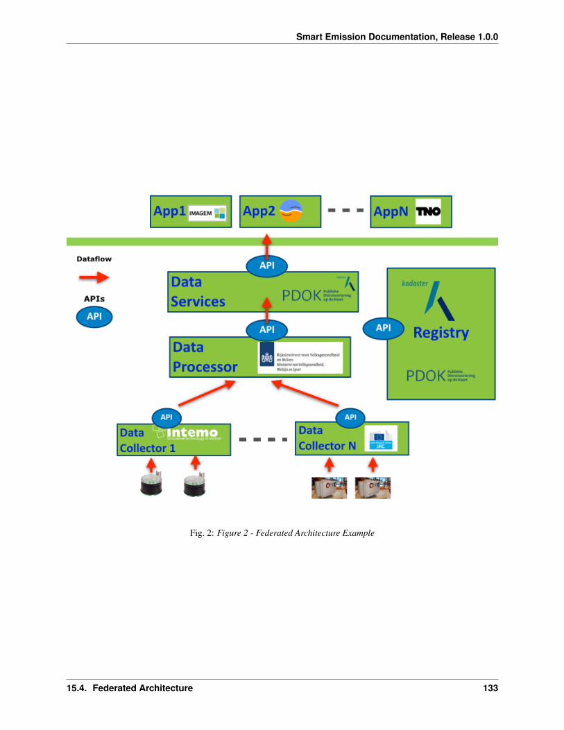
Smart Emission Documentation, Release 1.0.0
Fig. 2: Figure 2 - Federated Architecture Example
15.4. Federated Architecture 133
Smart Emission Documentation, Release 1.0.0
134 Chapter 15. Evolution
CHAPTER 16
Contact
The website www.smartemission.nl is the main entry point for this project.
The SE Data Platform has its own domain: data.smartemission.nl.
All development is done via GitHub: see https://github.com/smartemission/smartemission.
Developers for the SE Data Platform are Just van den Broecke (lead, document editor), Pieter Marsman (calibration),Thijs Brentjens
Contact Just van den Broecke at email at just AT justobjects.nl
135
Smart Emission Documentation, Release 1.0.0
136 Chapter 16. Contact
CHAPTER 17
Links
Below links relevant to the project.
17.1 Smart Emission
• Smart Emission Platform (PDF)
• Smart Emission - Building a Spatial Data Infrastructure for an Environmental Citizen Sensor Network
• Making sense of standards An evaluation and harmonisation of standards in the sensor web - M.C. Kastelijns(PDF)
• Emit #1+ – series of blog posts on SE Platform by Just van den Broecke on justobjects.nl
17.2 Sensors
• Luchtkwaliteit meten met sensoren - Joost Wesseling, Annemarie van Alphen, Hester Volten, Edith van Putten- RIVM, Statusoverzicht januari 2016
• https://www.samenmetenaanluchtkwaliteit.nl/apparaten-en-kits
• “Meetspecialisten praten elkaar bij over luchtsensoren” Presentaties op symposium Samen Meten 2017, o.a. JanVonk, Joost Wesseling (RIVM)
17.3 Calibration
• Field calibration of a cluster of low-cost available sensors for air quality monitoring. Part A: Ozone and nitrogendioxide - Laurent Spinelle, Michel Gerboles, Maria Gabriella Villani, Manuel Aleixandre, Fausto Bonavitacola
137
Smart Emission Documentation, Release 1.0.0
• Field calibration of a cluster of low-cost commercially available sensors for air quality monitoring. Part B:NO, CO and CO2 - Laurent Spinelle, Michel Gerboles, Maria Gabriella Villani, Manuel Aleixandre, FaustoBonavitacola
17.4 Education
• Geonovum Course Sensor_Web_Enablement (SWE) - http://geostandards.geonovum.nl/index.php?title=5_Sensor_Web_Enablement
• OGC SWE Architecture: http://docs.opengeospatial.org/wp/07-165r1/
• Wikipedia Sensor Web http://en.wikipedia.org/wiki/Sensor_web
• SensorThings: Geodan GOST presentatie FOSS4GUK : http://slides.com/bertt/gost_foss4guk#/
17.5 Data
• Landelijk Meetnet Luchtkwaliteit http://www.lml.rivm.nl/
• Ruwe LML XML data RIVM: http://geluid.rivm.nl/sos
• Download XML in IPR format: http://www.regione.piemonte.it/ambiente/aria/rilev/ariaday-test/xmlexport/read?startDate=&endDate=&action=selection
17.6 Europe
• European Environment Agency (EEA) http://www.eea.europa.eu/themes/air
• Eionet AQ Portal: http://www.eionet.europa.eu/aqportal/
• Directives 2004/107/EC and 2008/50/EC Implementing Decision - http://eur-lex.europa.eu/LexUriServ/LexUriServ.do?uri=OJ:L:2011:335:0086:0106:EN:PDF
• AirQualityReporting.xsd - http://dd.eionet.europa.eu/schema/id2011850eu-1.0/AirQualityReporting.xsd/view
17.7 Tools and Libs
• GDAL/OGR, http://gdal.org
• Stetl, Open Source ETL in Python, http://www.stetl.org
• Python Beautiful Soup : om HTML docs (bijv index.html Apache) uit te parsen: http://www.crummy.com/software/BeautifulSoup
• lxml, http://lxml.de
• deegree, http://www.deegree.org
• INSPIRE, http://inspire.ec.europa.eu/
• INSPIRE FOSS project, http://inspire-foss.org
• PostGIS/PostgreSQL, http://postgis.org
138 Chapter 17. Links
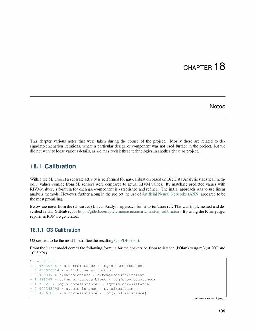
CHAPTER 18
Notes
This chapter various notes that were taken during the course of the project. Mostly these are related to de-sign/implemenation iterations, where a particular design or component was not used further in the project, but wedid not want to loose various details, as we may revisit these technologies in another phase or project.
18.1 Calibration
Within the SE project a separate activity is performed for gas-calibration based on Big Data Analysis statistical meth-ods. Values coming from SE sensors were compared to actual RIVM values. By matching predicted values withRIVM-values, a formula for each gas-component is established and refined. The initial approach was to use linearanalysis methods. However, further along in the project the use of Artificial Neural Networks (ANN) appeared to bethe most promising.
Below are notes from the (discarded) Linear Analysis approach for historic/future ref. This was implemented and de-scribed in this GitHub repo: https://github.com/pietermarsman/smartemission_calibration . By using the R-language,reports in PDF are generated.
18.1.1 O3 Calibration
O3 seemed to be the most linear. See the resulting O3 PDF report.
From the linear model comes the following formula for the conversion from resistance (kOhm) to ug/m3 (at 20C and1013 hPa)
O3 = 89.1177+ 0.03420626 * s.coresistance * log(s.o3resistance)- 0.008836714 * s.light.sensor.bottom- 0.02934928 s.coresistance * s.temperature.ambient- 1.439367 * s.temperature.ambient * log(s.coresistance)+ 1.26521 * log(s.coresistance) * sqrt(s.coresistance)- 0.000343098 * s.coresistance * s.no2resistance+ 0.02761877 * s.no2resistance * log(s.o3resistance)
(continues on next page)
139

Smart Emission Documentation, Release 1.0.0
(continued from previous page)
- 0.0002260495 * s.barometer * s.coresistance+ 0.0699428 * s.humidity+ 0.008435412 * s.temperature.unit * sqrt(s.no2resistance)
18.2 SOS Services
We tested istSOS at an early stage.
18.2.1 istSOS - Install Test
Notes from raw install as Python WSGI app, see also http://istsos.org/en/latest/doc/installation.html:
# as root$ mkdir /opt/istsos$ cd /opt/istsos# NB 2.3.0 gave problems, see https://sourceforge.net/p/istsos/tickets/41/$ wget https://sourceforge.net/projects/istsos/files/istsos-2.3.0.tar.gz$ tar xzvf istsos-2.3.0.tar.gz$ mv istsos 2.3.0$ ln -s 2.3.0 latest
$ chmod 755 -R /opt/istsos/latest$ chown -R www-data:www-data /opt/istsos/latest/services$ chown -R www-data:www-data /opt/istsos/latest/logs$ mkdir /opt/istsos/latest/wns # not present, need to create, no is for web→˓notification service$ chown -R www-data:www-data /opt/istsos/latest/wns # not present, gives error (?)
Add WSGI app to Apache conf.
Setup the PostGIS database.
$ sudo su - postgres$ createdb -E UTF8 -O sensors istsosPassword:$ psql -d istsos -c 'CREATE EXTENSION postgis'Password:CREATE EXTENSION
Restart and test:
$ service apache2 restart
# in browserhttp://api.smartemission.nl/istsos/admin/
# Database: fill in user/password
# create service (creates DB schema) "sound"
# test requestshttp://api.smartemission.nl/istsos/modules/requests/
(continues on next page)
140 Chapter 18. Notes

Smart Emission Documentation, Release 1.0.0
(continued from previous page)
# RESThttp://api.smartemission.nl/istsos/wa/istsos/services/sound
18.3 Fiware
Initially it was planned to run the SE platform on Fiware, but due to technical problems this was postponed and is stillon hold. Below some notes on installation.
The Fiware Lab NL provides a cloud-based computing infrastructure in particular for “Smart City” applications. Basedon the adopted “Docker-Strategy” for the Smart Emission Data Platform as described within the Architecture chapter,this chapter will describe the actual “hands-on” installation steps.
In order to start installing Docker images and other tooling we need to “bootstrap” the system within the Fiwareenvironment.
18.3.1 Fiware Lab NL
Creating a (Ubuntu) VM in the Fiware Lab NL goes as follows.
• login at http://login.fiware-lab.nl/
• create an SSL keypair via http://login.fiware-lab.nl/dashboard/project/access_and_security/
• create a VM-instance via http://login.fiware-lab.nl/dashboard/project/instances/ Launch Instance button
See the popup image above, do the following selections in the various tabs:
• Launch Instance tab: select boot from image, select base_ubuntu_14.04
• Access&Security tab: select keypair just created and enable all security groups
• Networking tab: assign both floating-IP and shared-net to selected networks
• other tabs: leave as is
• login via ssh -i <privkey_from_keypair>.pem ubuntu@<IP_address>
18.3. Fiware 141
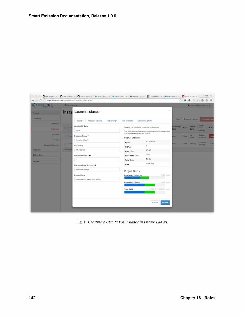
Smart Emission Documentation, Release 1.0.0
Fig. 1: Creating a Ubuntu VM instance in Fiware Lab NL
142 Chapter 18. Notes

CHAPTER 19
Indices and tables
• genindex
• modindex
• search
143