Soil Moisture Active Passive (SMAP)

Algorithm Theoretical Basis Document (ATBD)

SMAP Calibrated, Time-Ordered Brightness Temperatures L1B_TB Data Product

Initial Release, v.1

Jeffrey PiepmeierEd KimPriscilla MohammedJinzheng PengNASA Goddard Space Flight CenterGreenbelt, MD

Chris RufUniversity of MichiganAnn Arbor, MI

Algorithm Theoretical Basis Documents (ATBDs) provide the physical and mathematical descriptions of the algorithms used in the generation of science data products. The ATBDs include a description of variance and uncertainty estimates and considerations of calibration and validation, exception control and diagnostics. Internal and external data flows are also described.

The SMAP ATBDs were reviewed by a NASA Headquarters review panel in January 2012 and are currently at Initial Release, version 1. The ATBDs will undergo additional updates after the SMAP Algorithm Review in September 2013.

Contents1 Introduction..............................................................................................................................7

2 Overview and Background......................................................................................................7

2.1 Product/Algorithm Objectives..........................................................................................7

2.2 Historical Perspective.......................................................................................................8

2.3 Background and Science Objectives.................................................................................9

2.4 Measurement Approach....................................................................................................9

3 Instrument Description..........................................................................................................13

4 Forward Model (TB TA).....................................................................................................19

4.1 Brightness Temperature Forward Model........................................................................19

4.2 Radiometer System Forward Model...............................................................................22

4.2.1 Signal Through a Lossy Component.......................................................................22

4.2.2 Impedance Mismatch...............................................................................................23

4.2.3 Feed Network Lumped Loss Model........................................................................24

4.2.4 Forward Model to TA '.............................................................................................25

4.2.5 Forward Model to TA ' '............................................................................................26

4.2.6 Forward Model to TRFE..........................................................................................26

4.2.7 Radiometer Electronics Model................................................................................26

5 Baseline Retrieval Algorithm................................................................................................28

5.1 L1B_TB Algorithm Flow................................................................................................28

5.2 Level 1A Product............................................................................................................28

5.3 Geolocation and Pointing................................................................................................30

5.3.1 Long-term refinement of radiometer geolocation....................................................34

5.3.2 Radiometer geolocation and radar geolocation compatibility.................................35

5.4 Nonlinearity Correction..................................................................................................35

5.5 Calibration Coefficients Computation............................................................................36

5.6 Radiometric Calibration..................................................................................................36

5.6.1 Horizontal and Vertical Channels............................................................................36

5.6.2 Third and Fourth Stokes Parameters........................................................................38

5.7 Radio Frequency Interference (RFI)...............................................................................40

1

5.7.1 RFI Sources.............................................................................................................40

5.8 RFI Detection Algorithm Theory....................................................................................41

5.8.1 Pulse or Time Domain Detection............................................................................41

5.8.2 Cross Frequency Detection......................................................................................42

5.8.3 Kurtosis Detection...................................................................................................42

5.8.4 Polarimetric detection..............................................................................................43

5.8.5 RFI Model................................................................................................................43

5.8.6 FAR and PD of Detection Algorithms.....................................................................47

5.8.7 Area Under Curve (AUC) Parameterization............................................................49

5.9 Baseline Detection Algorithms.......................................................................................51

5.9.1 Time domain RFI detection.....................................................................................51

5.9.2 Cross-frequency RFI detection................................................................................52

5.9.3 Kurtosis Detection...................................................................................................53

5.9.4 T3 and T4 RFI detection...........................................................................................55

5.10 RFI Removal and Footprint Averaging.......................................................................55

5.10.1 Algorithm Implementation Details..........................................................................56

5.10.2 Detection Algorithm................................................................................................56

5.10.3 Mitigation Algorithm...............................................................................................57

5.10.4 RFI Flags.................................................................................................................58

5.11 RFI Detection and Removal from Calibration Data....................................................58

5.12 Antenna Pattern Correction.........................................................................................58

5.12.1 General approach.....................................................................................................60

5.12.2 APC including emissive main reflector...................................................................61

5.12.3 Galactic and CMB direct and reflected contribution...............................................63

5.12.4 Main Reflector Spillover and Feedthrough.............................................................63

5.12.5 Computation of contributions from Earth-viewing sidelobes and space view........63

5.13 Faraday Rotation.........................................................................................................63

5.13.1 Faraday rotation correction using T3 measurements (Option 1)..............................64

5.13.2 Faraday rotation correction using TEC and B-field data (Option2)........................65

5.13.3 Baseline Faraday correction approach.....................................................................66

5.14 Atmospheric Correction..............................................................................................66

2

5.15 Full transformation from antenna temperature TA to brightness temperature TB........67

6 Orbital Simulator...................................................................................................................68

6.1 Number of antenna beams...............................................................................................68

6.2 Conical scan....................................................................................................................68

6.3 Antenna pattern...............................................................................................................69

6.4 Land focus.......................................................................................................................69

6.5 Atmosphere model..........................................................................................................69

6.6 Ancillary data..................................................................................................................69

7 Calibration and Validation.....................................................................................................70

7.1 Pre-Launch Cal/Val (Antenna Temperature)..................................................................70

7.2 Post-Launch Cal/Val (Brightness Temperature).............................................................70

7.2.1 Geolocation Validation............................................................................................70

7.2.2 End-to-end TB Calibration Using External Targets.................................................70

7.3 Cold sky calibration........................................................................................................71

7.3.1 Purpose....................................................................................................................71

7.3.2 Temporal frequency.................................................................................................72

7.3.3 Sequence of maneuver.............................................................................................72

7.4 Subband vs. Fullband cross-calibration..........................................................................73

7.5 Scan bias correction........................................................................................................73

7.6 Drift detection and correction.........................................................................................73

7.7 Other post-launch cal/val activities.................................................................................73

7.7.1 General trending......................................................................................................73

7.7.2 Comparison of measured versus expected TB.........................................................74

7.7.3 Intercomparison versus other radiometers...............................................................74

8 Practical Considerations........................................................................................................74

8.1.1 Variance and Uncertainty Estimates........................................................................74

8.1.2 Test Plan..................................................................................................................75

9 References..............................................................................................................................77

3

Acronyms

µs – microsecondsAMR – Advanced Microwave RadiometerAPC – Antenna Pattern CorrectionAUC – Area Under CurveCMB – Cosmic Microwave BackgroundCNS – Correlated Noise SourceCW – Continuous WaveEESS – Earth Exploration Satellite ServiceEFOV – Effective Field of ViewEIA – Earth Incidence AngleEOS – Earth Observing System FAR – False Alarm RateFPGA – Field-Programmable Gate ArrayGDS – Ground Data SystemGSFC – Goddard Space Flight CenterIFOV – Instantaneous Field of ViewIGRF – International Geomagnetic Reference FieldIRI – International Reference IonosphereJPL – Jet Propulsion LaboratoryMPD – Maximum Probability of Detectionms – millisecondsNAIF - Navigation and Ancillary Information FacilityNCCS – NASA Center for Climate SimulationNCDC – National Climatic Data Center NEΔT – Noise Equivalent Differential TemperatureNEk – Noise Equivalent Differential kurtosisNOAA – National Oceanic and Atmospheric AdministrationNRC – National Research CouncilOMT – Ortho Mode TransducerOOB – Out Of BandPD – Probability of Detectionpdf – probability density functionPI – Principal InvestigatorPRF – Pulse Repetition FrequencyPRI – Pulse Repetition IntervalRBE – RF Back EndRDE – Radiometer Digital Electronics

4

RFE – Radiometer Front EndRFI – Radio Frequency InterferenceRMS – Root Mean SquareROC – Receiver Operating CurveSMAP – Soil Moisture Active PassiveSMAPVEX08 – Soil Moisture Active Passive Validation Experiment 2008SMOS – Soil Moisture and Ocean SalinitySPICE – Spacecraft ephemeris, Planet, satellite, comet, or asteroid ephemerides, Instrument description kernel, Pointing kernel, Events kernelSSS – Sea Surface SalinitySST – Sea Surface TemperatureTBC – To Be ConfirmedTBD – To Be DeterminedTEC – Total Electron ContentUSGS – United States Geological SurveyWGS84 – World Geodetic System 84

5

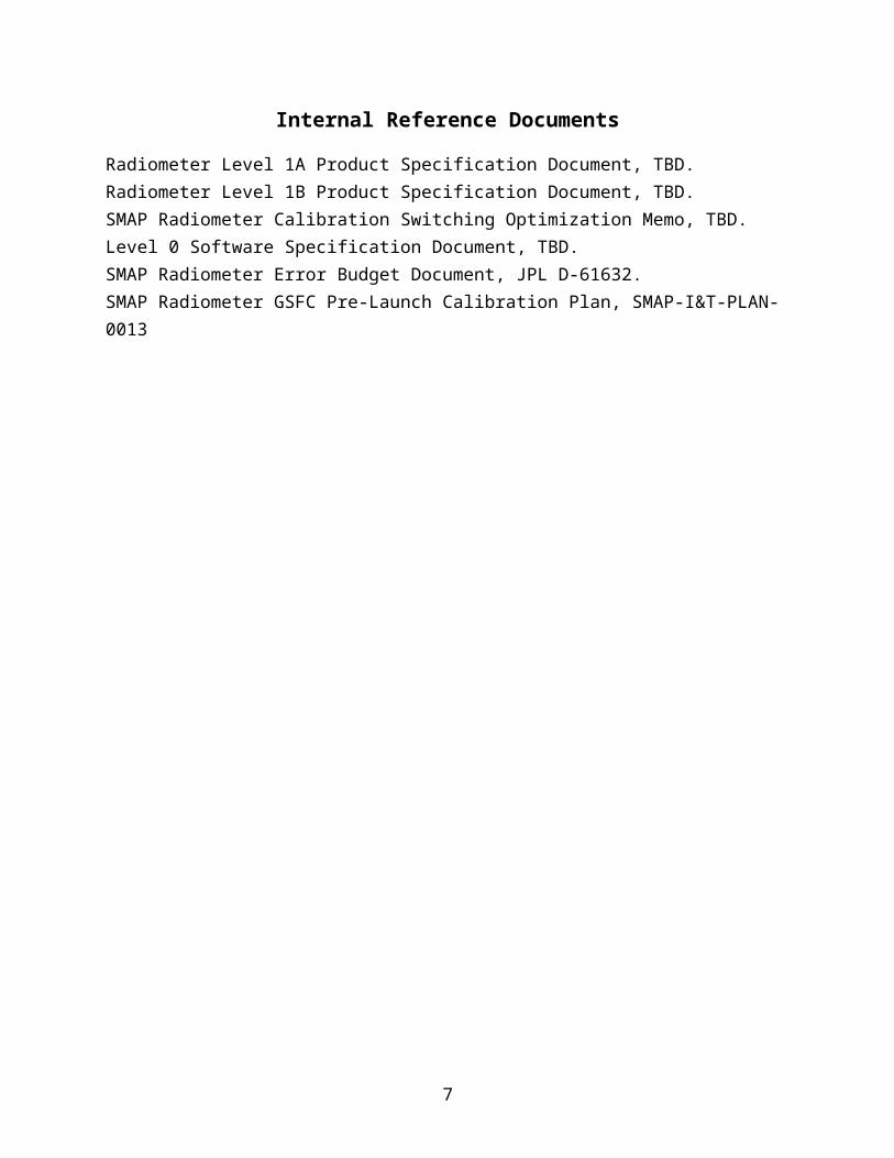
Internal Reference Documents

Radiometer Level 1A Product Specification Document, TBD.Radiometer Level 1B Product Specification Document, TBD.SMAP Radiometer Calibration Switching Optimization Memo, TBD.Level 0 Software Specification Document, TBD.SMAP Radiometer Error Budget Document, JPL D-61632.SMAP Radiometer GSFC Pre-Launch Calibration Plan, SMAP-I&T-PLAN-0013

6

1 Introduction

7

The purpose of the Soil Moisture Active Passive (SMAP) radiometer calibration algorithm is to convert L0 radiometer digital counts data into calibrated estimates of brightness temperatures within the main beam referenced to the Earth's surface. The algorithm theory in most respects is similar to what has been developed and implemented for decades for other satellite radiometers; however, SMAP includes two key features heretofore absent from satellite borne radiometers: radio frequency interference (RFI) detection and mitigation, and measurement of the third and fourth Stokes parameters using digital correlation.

The purpose of this document is to describe the SMAP radiometer and forward model; explain the SMAP calibration algorithm, including approximations, errors, and biases; provide all necessary equations for implementing the calibration algorithm; and, detail the RFI detection and mitigation process.

Section 2 provides a summary of algorithm objectives and driving requirements. Section 3 is a description of the instrument and Section 4 covers the forward models, upon which the algorithm is based. Section 5 gives the retrieval algorithm and theory. Section 6 describes the orbit simulator, which implements the forward model and is the key for deriving antenna pattern correction coefficients and testing the overall algorithm.

2 Overview and Background

2.1 Product/Algorithm ObjectivesThe objective of the Level 1B_TB algorithm is to convert radiometer digital counts to time ordered, geolocated brightness temperatures, TB. The raw counts are converted to TB producing two radiometer products that will be archived: Level 1A and Level 1B. The inputs to the L1B_TB algorithm are L0B data, which are raw radiometer telemetry output with repeats removed, unpacked and parsed. This preprocessing is handled separately to the L1B_TB algorithm. The algorithm will produce a Level 1A product in accordance with the EOS (Earth Observing System) Data Product Levels definition, which states that Level 1A data products are reconstructed, unprocessed instrument data at full resolution, time-referenced and annotated with ancillary information. The Level 1A product is a time-ordered series of instrument counts and includes housekeeping telemetry converted to engineering units for each scan. Geolocation and radiometric calibration are then performed on the Level 1A data to obtain antenna temperature, TA, followed by RFI detection algorithms which are used to detect and flag RFI. At this point RFI is removed and the data are time and frequency averaged near the antenna’s angular Nyquist rate. Finally, to compute the Level 1B product (time-ordered geolocated TB), radiometric error sources need to be removed such as those due to Faraday rotation, antenna sidelobes and spillover, solar radiation, cosmic microwave background and galactic emission. The driving requirements which directly affect the algorithm objectives are summarized in Table 1.

Table 1. Main requirements which affect the algorithm

8

Driving Requirements ID ParentSMAP shall provide a Level 1A time-ordered radiometer data product (L1A_Radiometer).

L2-SR-345

SMAP shall provide a Level 1B time-ordered radiometer brightness temperature product (L1B_TB) at 40 km spatial resolution.

L2-SR-268

The SMAP radiometer shall measure H, V, and 3 rd and 4th Stokes parameter brightness temperatures.

L2-SR-34

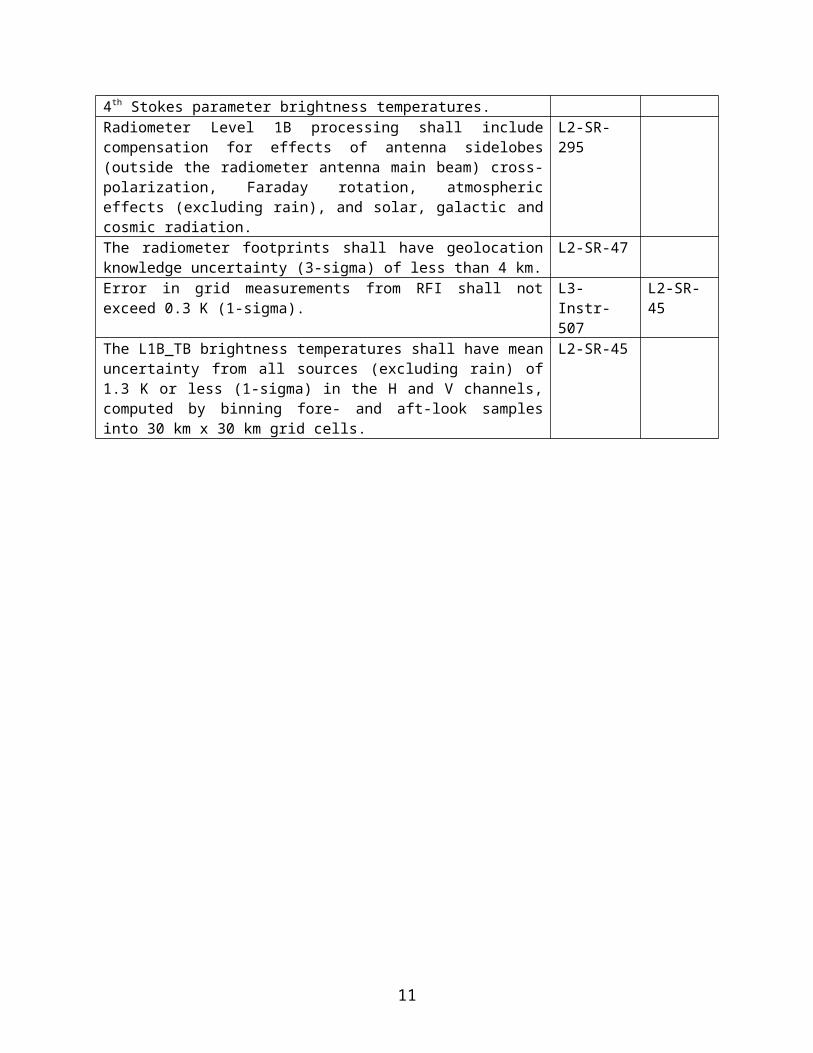
Radiometer Level 1B processing shall include compensation for effects of antenna sidelobes (outside the radiometer antenna main beam) cross-polarization, Faraday rotation, atmospheric effects (excluding rain), and solar, galactic and cosmic radiation.

L2-SR-295

The radiometer footprints shall have geolocation knowledge uncertainty (3-sigma) of less than 4 km.

L2-SR-47

Error in grid measurements from RFI shall not exceed 0.3 K (1-sigma). L3-Instr-507 L2-SR-45The L1B_TB brightness temperatures shall have mean uncertainty from all sources (excluding rain) of 1.3 K or less (1-sigma) in the H and V channels, computed by binning fore- and aft-look samples into 30 km x 30 km grid cells.

L2-SR-45

9

2.2 Historical PerspectiveThe Soil Moisture Active Passive (SMAP) mission was developed in response to the National Research Council’s (NRC) Earth Science and Applications from Space: National Imperatives for the Next Decade and Beyond (aka “Earth Science Decadal Survey,” NRC, 2007). SMAP will provide global measurements of soil moisture and freeze/thaw state using L-band radar and radiometry. SMAP has significant roots in the Hydrosphere State (Hydros) Earth System Science Pathfinder mission, which was selected as an alternate ESSP and subsequently cancelled in late 2005 prior to Phase A. One significant feature SMAP adopted from Hydros is the footprint oversampling used to mitigate RFI from terrestrial radars. The Aquarius/SAC-D project, a NASA ESSP ocean salinity mission launched in June 2011, also influenced the SMAP hardware and calibration algorithm. The radiometer front-end design is very similar to Aquarius; for example, the external correlated noise source (CNS) is nearly an exact copy of that from Aquarius. Features of the Aquarius calibration algorithm, such as calibration averaging and extra-terrestrial radiation source corrections, are incorporated into the SMAP algorithm. Finally, the SMAP orbit simulator is a modification of the Aquarius simulator code. SMAP’s antenna is conical scanning with a full 360-degree field of regard. However, there are several key differences (some unique) from previous conical scanning radiometers. Most obvious is the lack of external warm-load and cold-space reflectors, which normally provide radiometric calibration through the feedhorn. Rather, SMAP’s internal calibration scheme is based on the Aquarius/SAC-D and Jason Advanced Microwave Radiometer (AMR) pushbroom radiometers, and uses a reference load switch and a coupled noise diode. The antenna system is shared with the SMAP radar, which requires the use of a frequency diplexer in the feed network. Like WindSat, SMAP measures all four Stokes parameters, although unlike WindSat, SMAP uses coherent detection in a digital radiometer backend. The first two modified Stokes parameters, TV

and TH, are the primary science channels; the T3 and T4 channels are used to help detect RFI, which has recently proven quite valuable for the SMOS mission [Skou et. al 2010]. The T3

channel measurement can also provide correction of Faraday rotation caused by the ionosphere. Finally, the most significant difference SMAP has from all past spaceborne radiometer

programs is its aggressive hardware and algorithm approach to RFI mitigation, which is discussed in Section 3.

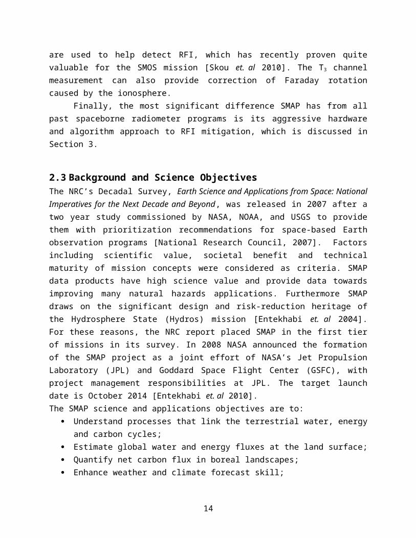
2.3 Background and Science ObjectivesThe NRC’s Decadal Survey, Earth Science and Applications from Space: National Imperatives for the Next Decade and Beyond, was released in 2007 after a two year study commissioned by NASA, NOAA, and USGS to provide them with prioritization recommendations for space-based Earth observation programs [National Research Council, 2007]. Factors including scientific value, societal benefit and technical maturity of mission concepts were considered as criteria. SMAP data products have high science value and provide data towards improving many natural

10

hazards applications. Furthermore SMAP draws on the significant design and risk-reduction heritage of the Hydrosphere State (Hydros) mission [Entekhabi et. al 2004]. For these reasons, the NRC report placed SMAP in the first tier of missions in its survey. In 2008 NASA announced the formation of the SMAP project as a joint effort of NASA’s Jet Propulsion Laboratory (JPL) and Goddard Space Flight Center (GSFC), with project management responsibilities at JPL. The target launch date is October 2014 [Entekhabi et. al 2010]. The SMAP science and applications objectives are to:

Understand processes that link the terrestrial water, energy and carbon cycles; Estimate global water and energy fluxes at the land surface; Quantify net carbon flux in boreal landscapes; Enhance weather and climate forecast skill; Develop improved flood prediction and drought monitoring capability

2.4 Measurement Approach

is a summary of the SMAP instrument functional requirements derived from its science measurement needs. The goal is to combine the attributes of the radar and radiometer observations (in terms of their spatial resolution and sensitivity to soil moisture, surface roughness, and vegetation) to estimate soil moisture at a resolution of 10 km, and freeze-thaw state at a resolution of 1-3 km.

The SMAP instrument incorporates an L-band radar and an L-band radiometer that share a single feedhorn and parabolic mesh reflector. As shown in Figure 1 the reflector is offset from nadir and rotates about the nadir axis at 14.6 rpm (nominal), providing a conically scanning antenna beam with a surface incidence angle of approximately 40°. The provision of constant incidence angle across the swath simplifies the data processing and enables accurate repeat-pass estimation of soil moisture and freeze/thaw change. The reflector has a diameter of 6 m, providing a radiometer 3 dB antenna footprint of 40 km (root-ellipsoidal-area). The real-aperture radar footprint is 30 km, defined by the two-way antenna beamwidth. The real-aperture radar and radiometer data will be collected globally during both ascending and descending passes.

To obtain the desired high spatial resolution the radar employs range and Doppler discrimination. The radar data can be processed to yield resolution enhancement to 1-3 km spatial resolution over the 70% outer parts of the 1000 km swath. Data volume prohibits the downlink of the entire radar data acquisition. Radar measurements that allow high-resolution processing will be collected during the morning overpass over all land regions and extending one swath width over the surrounding oceans. During the evening overpass data poleward of 45° N will be collected and processed as well to support robust detection of landscape freeze/thaw transitions.The baseline orbit parameters are:

Orbit Altitude: 685 km (2-3 days average revisit and 8-days exact repeat)

11

Inclination: 98 degrees, sun-synchronous Local Time of Ascending Node: 6 pm

Table 2. SMAP Mission Requirements

Scientific Measurement Requirements Instrument Functional RequirementsSoil Moisture:~0.04 m3m-3 volumetric accuracy(1-sigma) in the top 5 cm for vegetation water content ≤ 5 kg m-2;Hydrometeorology at ~10 km resolution;Hydroclimatology at ~40 km resolution

L-Band Radiometer (1.41 GHz):Polarization: V, H, T3 and T4

Resolution: 40 kmRadiometric Uncertainty*: 1.3 KL-Band Radar (1.26 and 1.29 GHz):Polarization: VV, HH, HV (or VH)Resolution: 10 kmRelative accuracy*: 0.5 dB (VV and HH)Constant incidence angle** between 35° and 50°

Freeze/Thaw State:Capture freeze/thaw state transitions in integrated vegetation-soil continuum with two-day precision, at the spatial scale of land-scape variability (~3 km).

L-Band Radar (1.26 GHz and 1.29 GHz):Polarization: HHResolution: 3 kmRelative accuracy*: 0.7 dB (1 dB per channel if 2 channels are used)Constant incidence angle** between 35° and 50°

Sample diurnal cycle at consistent time of day (6am/6pm Equator crossing);Global, ~3 day (or better) revisit;Boreal, ~2 day (or better) revisit

Swath Width: ~1000 km

Minimize Faraday rotation (degradation factor at L-band)

Observation over minimum of three annual cycles Baseline three-year mission life* Includes precision and calibration stability** Defined without regard to local topographic variation

The SMAP radiometer measures the four Stokes parameters, TV, TH, T3, and T4 at 1.41 GHz. The T3 channel measurement can be used to correct for possible Faraday rotation caused by the ionosphere, although such Faraday rotation is minimized by the selection of the 6 am/6 pm sun-synchronous SMAP orbit.

At L-band anthropogenic Radio Frequency Interference (RFI), principally from ground-based surveillance radars, can contaminate both radar and radiometer measurements. Early measurements and results from the SMOS mission indicate that in some regions RFI is present and detectable. The SMAP radar and radiometer electronics and algorithms have been designed to include features to mitigate the effects of RFI. To combat this, the SMAP radar utilizes selective filters and an adjustable carrier frequency in order to tune to pre-determined RFI-free portions of the spectrum while on orbit. The SMAP radiometer will implement a combination of time and frequency diversity, kurtosis detection, and use of T4 thresholds to detect and where possible mitigate RFI.

12

The SMAP planned data products are listed in Table 3. Level 1B and 1C data products are calibrated and geolocated instrument measurements of surface radar backscatter cross-section and brightness temperatures derived from antenna temperatures. Level 2 products are geophysical retrievals of soil moisture on a fixed Earth grid based on Level 1 products and ancillary information; the Level 2 products are output on half-orbit basis. Level 3 products are daily composites of Level 2 surface soil moisture and freeze/thaw state data. Level 4 products are model-derived value-added data products that support key SMAP applications and more directly address the driving science questions.

Figure 1. The SMAP observatory is a dedicated spacecraft with a rotating 6 m light weight deployable mesh reflector. The radar and radiometer share a common feed.

Table 3. SMAP Data Products Table.

13

14

3 Instrument DescriptionThe SMAP instrument architecture consists of a 6-meter, conically-scanning reflector antenna and a common L-band feed shared by the radar and radiometer (see Figure 2). The reflector rotates about the nadir axis at a stable rate which can be set in the range between 13 – 14.6 rpm, producing a conically scanning antenna beam with approximately 40 km 3-dB footprint at the surface with an Earth incidence angle of approximately 40 degrees. The nominal integration times and footprint size in this document are based on a spin rate of 14.6 rpm. The conical scanning sweeps out a 1000-km wide swath with both fore and aft looks for the radiometer (see Figure 3).

Figure 2. Spun instrument configuration

15

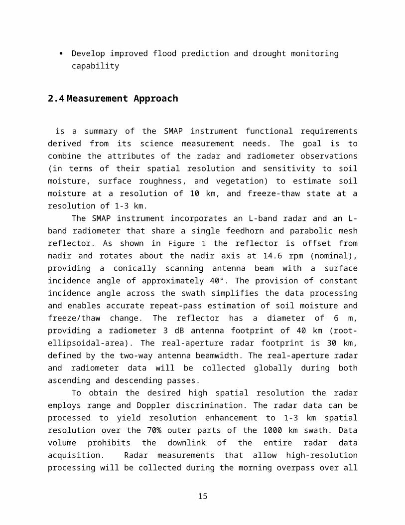
Figure 3. SMAP measurement geometry showing radiometer swath, and high- and low-resolution radar swaths.

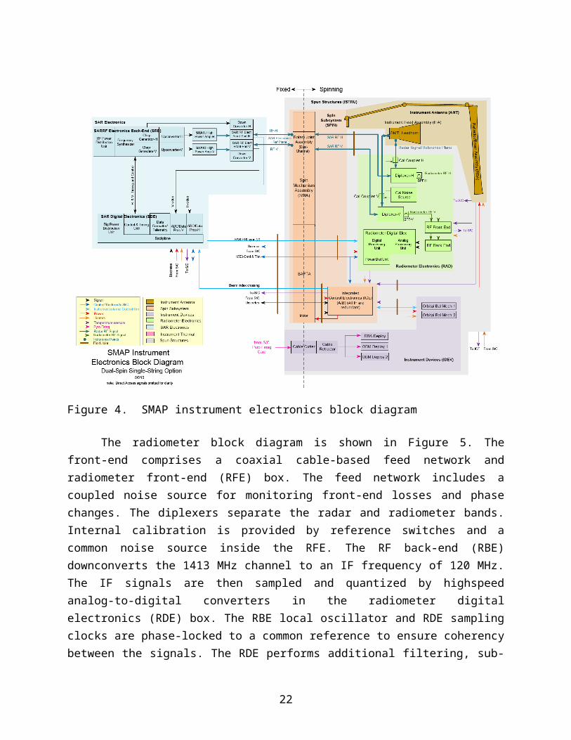
The instrument block diagram, showing the antenna, radar, and radiometer, is in Figure 4. The feed assembly employs a single horn, ortho-mode transducer, with V and H polarizations aligned with the Earth’s natural polarization basis, and is made dual frequency with the use of a diplexer within the coaxial cable-based feed network. The radiometer uses 24 MHz of bandwidth centered at 1.4135 GHz, while the radar can frequency hop between 1215 and 1300 MHz. The radar and radiometer frequencies will be separated by diplexers and routed to the appropriate electronics for detection. The radiometer electronics are located on the spun side of the interface (see inset in Figure 2). Slip rings provide a signal interface to the spacecraft. The more massive and more thermally dissipative electronics of the radar are on the despun side, and the transmit/receive pulses are routed to the spun side via a two-channel RF rotary joint. The radiometer timing for the internal calibration switching and detection integrators is synchronized with the radar transmit/receive timing to provide additional RF compatibility between the radar and radiometer and to ensure co-alignment of the brightness temperature and backscatter cross-section measurements.

1000 km

16

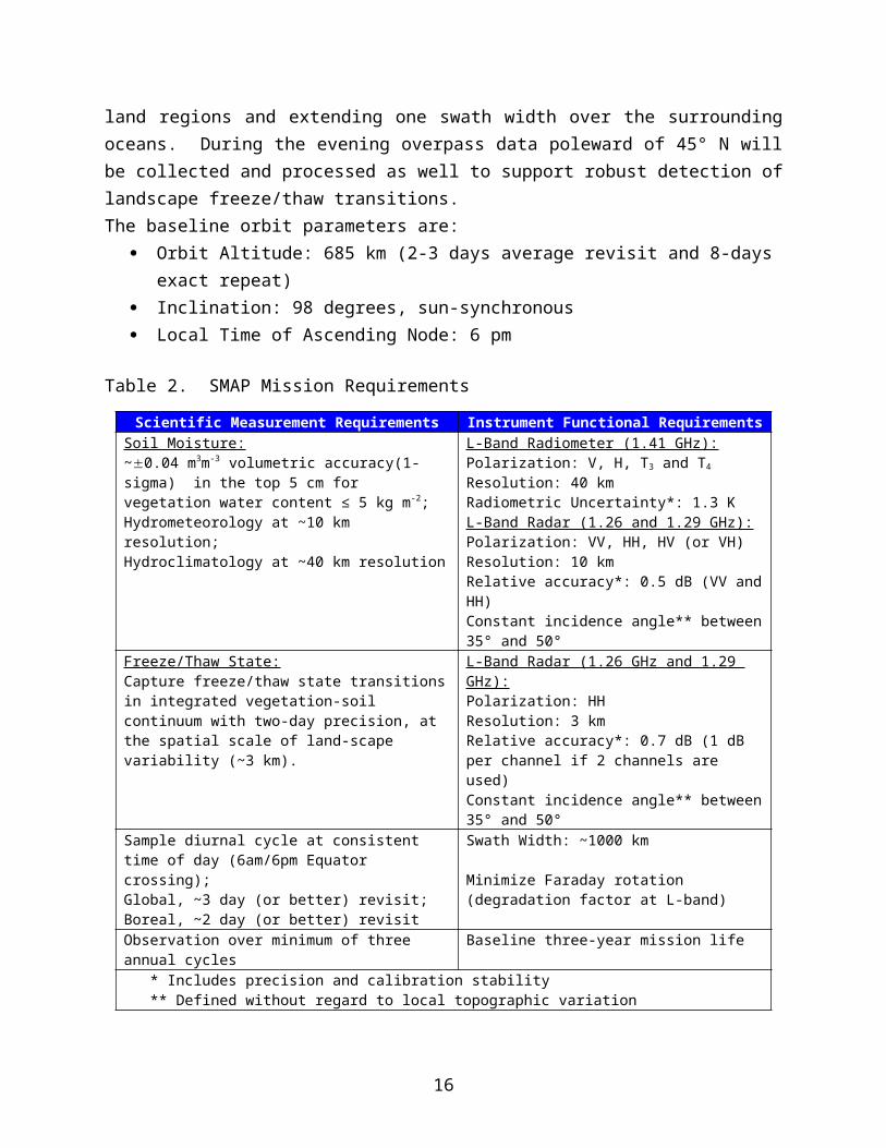
Figure 4. SMAP instrument electronics block diagram

The radiometer block diagram is shown in Figure 5. The front-end comprises a coaxial cable-based feed network and radiometer front-end (RFE) box. The feed network includes a coupled noise source for monitoring front-end losses and phase changes. The diplexers separate the radar and radiometer bands. Internal calibration is provided by reference switches and a common noise source inside the RFE. The RF back-end (RBE) downconverts the 1413 MHz channel to an IF frequency of 120 MHz. The IF signals are then sampled and quantized by highspeed analog-to-digital converters in the radiometer digital electronics (RDE) box. The RBE local oscillator and RDE sampling clocks are phase-locked to a common reference to ensure coherency between the signals. The RDE performs additional filtering, sub-band channelization, cross-correlation for measuring T3 and T4, and detection and integration of the first four raw moments of the signals. These data are packetized and sent to the ground for calibration and further processing.

17

Figure 5. Block diagram of radiometer

Figure 6. Radiometer Timing

COUPCNS

Noise SRC

Pwr Cond

HKCMD/CTRL

RF Mon’sRFE

Analog Processing& A/D

FPGA BasedDigital Signal Processing

FPGA BasedTiming, CMD,

TLM& Packetization

I/FCktsHK

DC-DC Conv with EMI Filtering

CMN MD Filtering and HK Meas

S/C

RADAR

S/CPWR

RDE

PDU

RDE HK

COUP DIP

RBE

RF Chain with Ref Switch

CLK

Down-Conv

Down-Conv

RF Chain with Ref Switch

DIP

RADAR

PWRCond

PLO

SLIPRINGASSY

RFIF

IFRF

OSC

1.4 GHzRadiometer

18

The radiometer timing diagram is show in Figure 6. For every pulse repetition interval (PRI) of the radar, the radiometer integrates for ~300 µs during the receive window. (The exact amount of time can vary based on the radar PRI length and blanking time length chosen by the instrument designers.) Radiometer packets are made up of 4 PRIs. As shown in Table 4, each science data packet includes fullband, or time domain, data for each of the four PRIs; and subbanded data, which have been further integrated to 4 PRIs or ~1.2 ms. The science telemetry includes the first four sample raw moments of the fullband (24-MHz wide) and 16 subband (each 1.5 MHz wide) signals, for both polarizations and separately expressed in terms of the in-phase and quadrature components of the signals. The 3rd and 4th Stokes parameters are also produced via complex cross-correlation of the two polarizations for the fullband as well as each of the 16 subbands. Every science data packet therefore contains 360 pieces of time-frequency data.

Table 4. Radiometer science dataInt. time Pol Channel Moment Pol Channel Moment Pol Channel Pol Channel

300 µs V Fulband 1-4, I,Q H Fulband 1-4, I,Q 3 Fulband 4 Fulband300 µs V Fulband 1-4, I,Q H Fulband 1-4, I,Q 3 Fulband 4 Fulband300 µs V Fulband 1-4, I,Q H Fulband 1-4, I,Q 3 Fulband 4 Fulband300 µs V Fulband 1-4, I,Q H Fulband 1-4, I,Q 3 Fulband 4 Fulband1.2 ms V 1 1-4, I,Q H 1 1-4, I,Q 3 1 4 11.2 ms V 2 1-4, I,Q H 2 1-4, I,Q 3 2 4 21.2 ms V 3 1-4, I,Q H 3 1-4, I,Q 3 3 4 31.2 ms V 4 1-4, I,Q H 4 1-4, I,Q 3 4 4 41.2 ms V 5 1-4, I,Q H 5 1-4, I,Q 3 5 4 51.2 ms V 6 1-4, I,Q H 6 1-4, I,Q 3 6 4 61.2 ms V 7 1-4, I,Q H 7 1-4, I,Q 3 7 4 71.2 ms V 8 1-4, I,Q H 8 1-4, I,Q 3 8 4 81.2 ms V 9 1-4, I,Q H 9 1-4, I,Q 3 9 4 91.2 ms V 10 1-4, I,Q H 10 1-4, I,Q 3 10 4 101.2 ms V 11 1-4, I,Q H 11 1-4, I,Q 3 11 4 111.2 ms V 12 1-4, I,Q H 12 1-4, I,Q 3 12 4 121.2 ms V 13 1-4, I,Q H 13 1-4, I,Q 3 13 4 131.2 ms V 14 1-4, I,Q H 14 1-4, I,Q 3 14 4 141.2 ms V 15 1-4, I,Q H 15 1-4, I,Q 3 15 4 151.2 ms V 16 1-4, I,Q H 16 1-4, I,Q 3 16 4 16

A radiometer footprint is defined to be 12 packets long, 11 of which are for observing the scene and the 12th for internal calibration. Figure 7(a) shows the formation of a footprint in terms of 3-dB contours. Integration of the 11 observing packets slightly enlarges the antenna’s instantaneous field-of-view (IFOV) from 36 km x 47 km to an effective field-of-view (EFOV) of 39 km x 47 km. The EFOV spacing shown in Figure 7(b) is approximately 11 km x 31 km near the swath center.

19

(a)

(b)

Figure 7. Radiometer EFOV formation (a) and spacing (b).

20

4 Forward Model (TB TA)

4.1 Brightness Temperature Forward ModelIn this section, we describe the sources contributing to the total apparent temperature seen at the input to the SMAP main reflector.

The brightness temperature of a source (measured in Kelvin) can be described in terms of the product of the physical temperature and the emissivity of the source. Emissivity is, in general, polarization-dependent, thus differentiating brightness temperature into T B , V and T B , H for the vertical and horizontal polarizations, respectively. These are the first two modified Stokes parameters. The real part of the complex correlation between these two components is measured by the third modified Stokes parameter, represented in brightness temperatures as T3. The fourth Stokes parameter, T4 measures the imaginary part of the correlation. For this document, a vector of modified Stokes parameters is shown by

T B (θ , ϕ )=[T v

Th

T3

T 4]

(4.1)

where θ and ϕ are the elevation and azimuth of a spherical coordinate system centered on the radiometer antenna boresight vector.

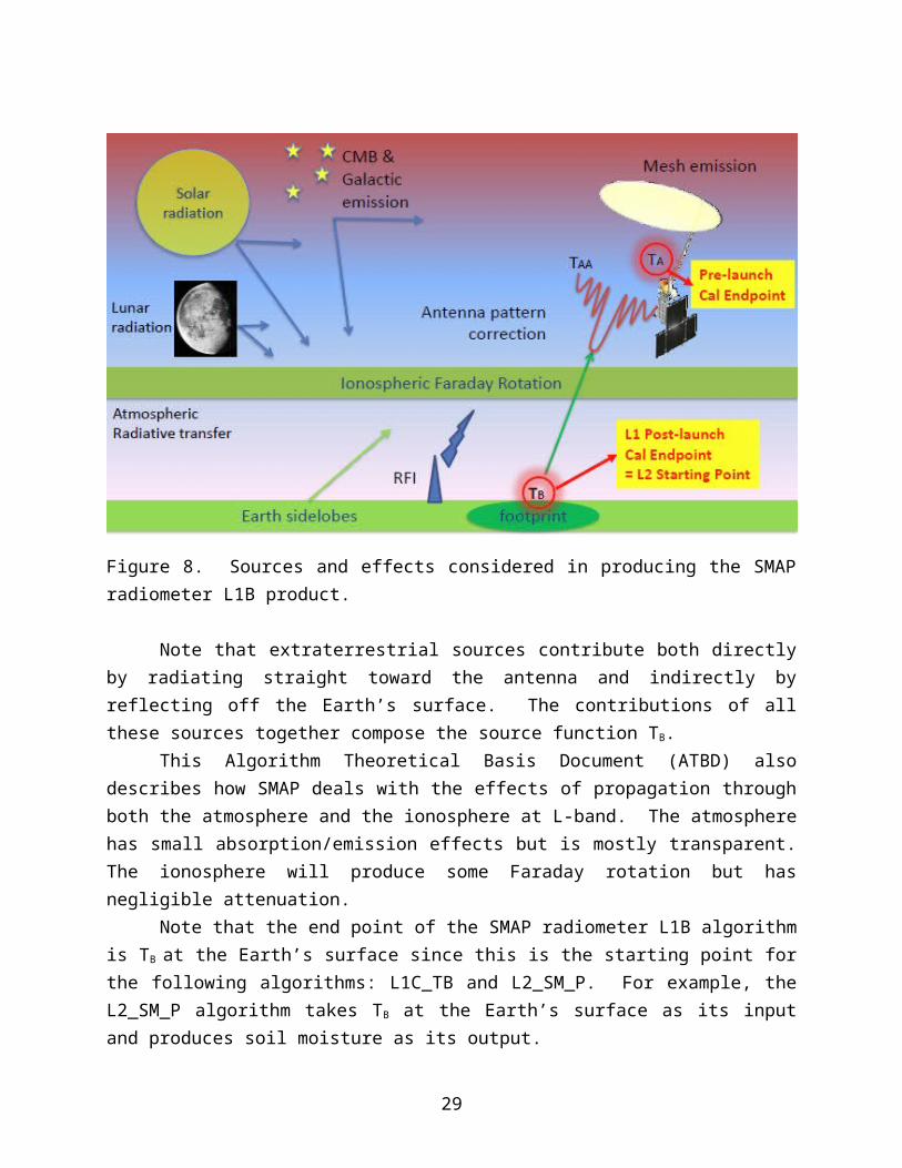
Important sources of radiation at L-band are the Earth’s land and sea, the cosmic background radiation, the sun, radiation sources outside our solar system, and the moon. Figure8 depicts the various sources and effects considered in producing the SMAP radiometer L1B product. More details are given in Section 5.12.

21

Figure 8. Sources and effects considered in producing the SMAP radiometer L1B product.

Note that extraterrestrial sources contribute both directly by radiating straight toward the antenna and indirectly by reflecting off the Earth’s surface. The contributions of all these sources together compose the source function TB.

This Algorithm Theoretical Basis Document (ATBD) also describes how SMAP deals with the effects of propagation through both the atmosphere and the ionosphere at L-band. The atmosphere has small absorption/emission effects but is mostly transparent. The ionosphere will produce some Faraday rotation but has negligible attenuation.

Note that the end point of the SMAP radiometer L1B algorithm is TB at the Earth’s surface since this is the starting point for the following algorithms: L1C_TB and L2_SM_P. For example, the L2_SM_P algorithm takes TB at the Earth’s surface as its input and produces soil moisture as its output.

When an electromagnetic radiation propagates through the Earth atmosphere, it is absorbed by the atmosphere. At the same time, the atmosphere emits energy which will become part of the radiation received by the space-borne radiometer. Three parameters (upwelling brightness Tup, downwelling brightness Tdown, and total atmospheric loss factor L) are needed to describe the atmosphere’s effect on the radiation which is emitted from or reflected by the Earth’s surface and received by a spaceborne radiometer. The general form of the apparent brightness temperature at the top of the atmosphere (TOA) is given by

22

T ap' =T up+ [ (1−ε )T down+T B ] L−1

(4.2)

where ε is the emissivity of the Earth’s surface and TB is the brightness temperature of the Earth’s surface. This equation simply says that the radiometer sees the sum of the surface brightness TB attenuated by L, added to upwelling atmospheric brightness Tup plus the downwelling atmospheric brightness Tdown reflected off the surface and attenuated by L. The atmosphere can change the polarization state of the radiation when it propagates through the ionosphere. The ionosphere acts as an anisotropic medium, which can alter the polarization state of the wave [Stratton, 1941; Kraus 1966]. For SMAP, for example, linearly-polarized signals transiting through the Earth’s ionosphere will experience some degree of polarization change. The amount of polarization rotation in this case can be expressed as

Ωf=2.62×10−13 λ2∫ ne B||ds (in radians)(4.3)

where λ is in meters, ne is electrons/m-3, B|| is the magnetic field component parallel to the propagation direction in teslas; integration is along the viewing path. λ = c/f = 0.21m, SMAP radiometer wavelength. The resulting apparent temperature incident on the SMAP main reflector becomes

[T ap ,v

T ap ,h

T ap ,3

T ap, 4]=[ Tap , v

' −∆T ap

T ap ,h' +∆ T ap

−(T ap , v' −T ap ,h

' )sin 2 Ωf +T ap ,3' cos2 Ωf

Tap , 4' ]

(4.4)

where T ap , x' (x = v, h, 3, 4) is the apparent brightness at TOA of polarization x; and

∆ T ap=(T ap, v' −T ap ,h

' )sin 2Ω f−T ap ,3

'

2sin 2 Ωf

(4.5)

Considering all of the radiation sources and all the incidence direction on the SMAP main reflector, the total Tap incident on the main reflector is

T ap=T ap , MB+T ap, ESA+T ap , SSA

(4.6)

where T ap , MB is the brightness incident through the main beam, T ap , ESAis the brightness incident through sidelobes that view the Earth (more precisely, the solid angle subtended by the Earth but not including the main beam, or the “Earth solid angle”), and T ap ,SSA is the brightness incident

23

through sidelobes that view off-Earth directions, including back lobe directions (i.e., all other directions, or the “space solid angle”). Together, the three terms on the right hand side of Equation (4.6) subtend the full 4π steradian solid angle around the main reflector.

We further split T ap , ESAand T ap ,SSA into components:

T ap , ESA=T ap , ESL+Tap ,⨀ ,refl+T ap ,moon ,refl+Tap , CMB, refl+T ap, gal ,refl

(4.7)

T ap ,SSA=T ap,⨀ ,dir+T ap ,moon ,dir+T ap, CMB, dir+T ap , gal ,dir

(4.8)

where T ap ,⨀ , refl ,T ap ,moon ,refl , T ap ,CMB ,refl ,∧T ap , gal, refl are brightness after reflection off the Earth into the Earth solid angle from, respectively, the sun, the moon, cosmic microwave background, and the galaxy. T ap , ESL accounts for Earth emission into sidelobes that view the Earth. With respect to Equation (4.8), T ap ,⨀ , dir , T ap, moon, dir , T ap ,CMB ,dir ,∧T ap ,gal , dir are brightness entering the space solid angle directly from, respectively, the sun, the moon, cosmic microwave background, and the galaxy. All Tap quantities in Equations (4.7) and (4.8) are, in general, 4-vectors corresponding to the 4 modified Stokes parameters (although we can treat T ap ,⨀ , dir , T ap, moon, dir , T ap ,CMB ,dir ,∧T ap ,gal , dir as unpolarized). All right hand terms in Equations (4.6) to (4.8) are integrals of the respective source TB over the indicated solid angle weighted by the SMAP antenna pattern in each direction (θ , ϕ )relative to the antenna boresight coordinate frame. As the antenna is constantly rotating, the terms in Equations (4.6) to (4.8) are all implicitly functions of the time of observation. Each also includes polarization basis rotations for Faraday rotation correction and alignment of the v-h basis with the main beam basis.

4.2 Radiometer System Forward ModelThe forward model traces the path of signal from feedhorn to the power digitally recorded in the radiometer.

4.2.1 Signal Through a Lossy ComponentThe antenna temperature of the signal in a radiometer is defined as

T=[T v

Th

T3

T 4] .

(4.9)

Assuming perfect isolation between the vertical and horizontal channels, a loss in the system will behave by attenuating the signals while inserting additional antenna power into the

24

vertical and horizontal channels based on the physical temperature of the ohmic loss. Thus, the antenna temperature vector T ' after loss L is

T '= L−1 T+( I− L−1 )T ph y

(4.10)

where L−1 is the Mueller matrix [Piepmeier et. al 2008] of the loss shown as

[Lv

−1 0 0 00 Lh

−1 0 0

0 0 ( Lv Lh )−12 0

0 0 0 ( Lv Lh )−12]

(4.11)

and T p h y is a physical temperature vector

T phy=[T phys , v

T phys , h

00 ]

(4.12)

where T phys ,v and T phys ,h are the physical temperatures of the loss in the vertical and horizontal channels.

4.2.2 Impedance MismatchAn impedance mismatch will attenuate a passing signal while reflecting outgoing noise back into the receiver. Ignoring the OMT cross-coupling which has been subsumed into the antenna pattern correction algorithm, channels v and h can be treated as total power channels and the effective signal into the receiver can be modeled as [Corbella et al. 2005]

T out= ¯M T in+T M(4.13)

where T in is input Stokes parameter vector

25

T in=[T v

Th

T3T 4

](4.14)

¯M=[|Λv|2 0 0 0

0 |Λh|2 0 0

0 0 Re Λv Λh¿ −Im Λv Λh

¿

0 0 Im Λv Λh¿ Re Λv Λh

¿ ](

4.15)

T M =[|Λv|2|Γa , v|

2T phy , iso , v+2 Re [ Λv Γa ,v T cor , v ]|Λh|

2|Γa , h|2T phy , iso , v+2 Re [ Λh Γa ,h T cor ,h ]

00

](4.16)

where T phy , iso , k (k = v, h) is the physical temperature of the isolator in receiving channel k; Γ a, k is the feedhorn assembly (including OMT) reflection coefficient of channel k and

Λk=1

1−S11, k Γ a,k(4.17)

T cor , k=−T phy ,iso , k (S11 ,TSFE ,k+S12 , TSFE ,k S22 ,TSFE , k

¿

S21 , TSFE, k¿ )

(4.18)

where S11 , k (k = v, h) is the input reflection coefficient of the receiver (channel k, started from CNS coupler); The S-parameters with subscript ‘TSFE’ are defined for the temperature sensitive front-end (TSFE) components: CNS coupler through RFE isolator. Physical temperatures of these TSFE components are assumed to be the same.

26

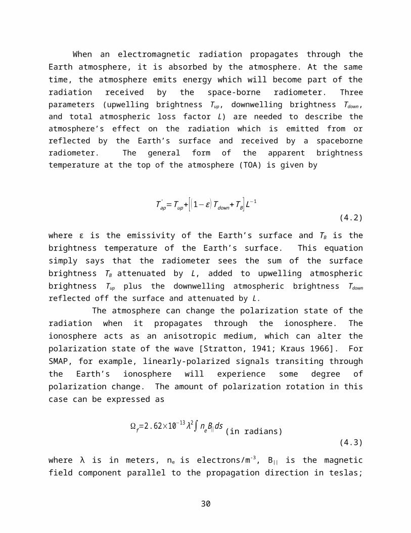
4.2.3 Feed Network Lumped Loss ModelA lumped loss model is used to derive the antenna temperature as measured at the input of the radiometer front end (RFE). The block diagram of the vertical and horizontal channels of the SMAP radiometer leads directly to lumped loss model shown in Figure 9 and its corresponding calibration model shown in Figure 10.

Figure 9. Lumped Loss Model

The lumped loss and phase offset model in Figure 9 produces a forward model to relate the antenna temperature incident on the antenna to the antenna temperature at the input to the RFE. This assumes minimal temperature gradients within each of these lumped losses. There are two phase imbalance matrices included. The first covers all phase imbalance up to the injected signal from the correlated noise diode. The second covers the remaining phase imbalance, and may be removed and lumped into the radiometer electronics phase imbalance.

T A' '

Feed Horn

L2 ,T L 2

OMT

L3 ,T L3

Γ

CNS Coupler

L4 , T L 4

P ( Δ ϕ1 )

Diplexer& BPF

L5 ,T L5

Phase Diff.

P ( Δ ϕ2 )

T A

CNS Injection+T CN

T A' T A

RFE

27

Figure 10. Calibration Model

4.2.4 Forward Model to T A'

The forward model from T AA to T A' is the stacking of the individual lumped loss elements

followed by the reflection as measured at the input to the OMT

T A' = L3

−1 L2−1T A+ L3

−1 ( I−L2−1 )T L 2+ ( I−L3

−1 )T L 3+.(4.19)

4.2.5 Forward Model to T A' '

The forward model from T A' to T A

' ' is the stacking of the individual lumped loss element followed by the net phase imbalance Mueller matrix

T A' '=P ( Δϕ1 ) L4

−1 T A' + ( I−L4

−1 )T L 4.(4.20)

4.2.6 Forward Model to T RFE

The forward model to T RFE depends on the state of the correlated noise diode. This leads to the two equations

T ARFE= P (∆ ϕ2 ) ( L5

−1T A' ' +( I−L5

−1 )T L5 ) ,∧CNSOFF

P (∆ ϕ2 ) ( L5−1 (T ' A

' +TCNS )+ ( I−L5−1 )T L5 ) ,∧CNS ON

(4.21)

where T CNS is the additive Stokes vector due to the correlated noise diode. It can be measured pre-launch or estimated as described in [Piepmeier and Kim, 2003].

The internal calibration network can produce eight different combinations of switch and noise diode states. The default radiometer switching sequence uses four of them. So the antenna temperature to the RFE input are numbered and listed below

T RFE(1)=T ref

(4.22)

T RFE (2 )=T ref +T ND

(4.23)

T RFE(3)=T ARFE

(4.24)

28

T RFE(4)=T ARFE+T ND

(4.25)

4.2.7 Radiometer Electronics ModelThere are two internal calibration sources inside the RFE for radiometer calibration. The internal calibration scheme designed into the RF electronics can be modeled as

[Cx , v

Cx , h

Cx , 3C x , 4

]=[G vv 0 0 00 Ghh 0 00 0 G33 G340 0 G43 G44

]T RFE+[Ov

Oh

O3O4

]+n

(4.26)

where C x , y (x=A, A+ND, ref, ref+ND; y=v, h, 3, 4) is radiometer output counts for output

channel y with calibration state x; G yγ (=v, h, 3, 4) is the forward gain coefficient for output

channel y corresponding to input ; O y is the radiometer offset coefficient for output channel y; n is the radiometer random noise.

29

5 Baseline Retrieval Algorithm

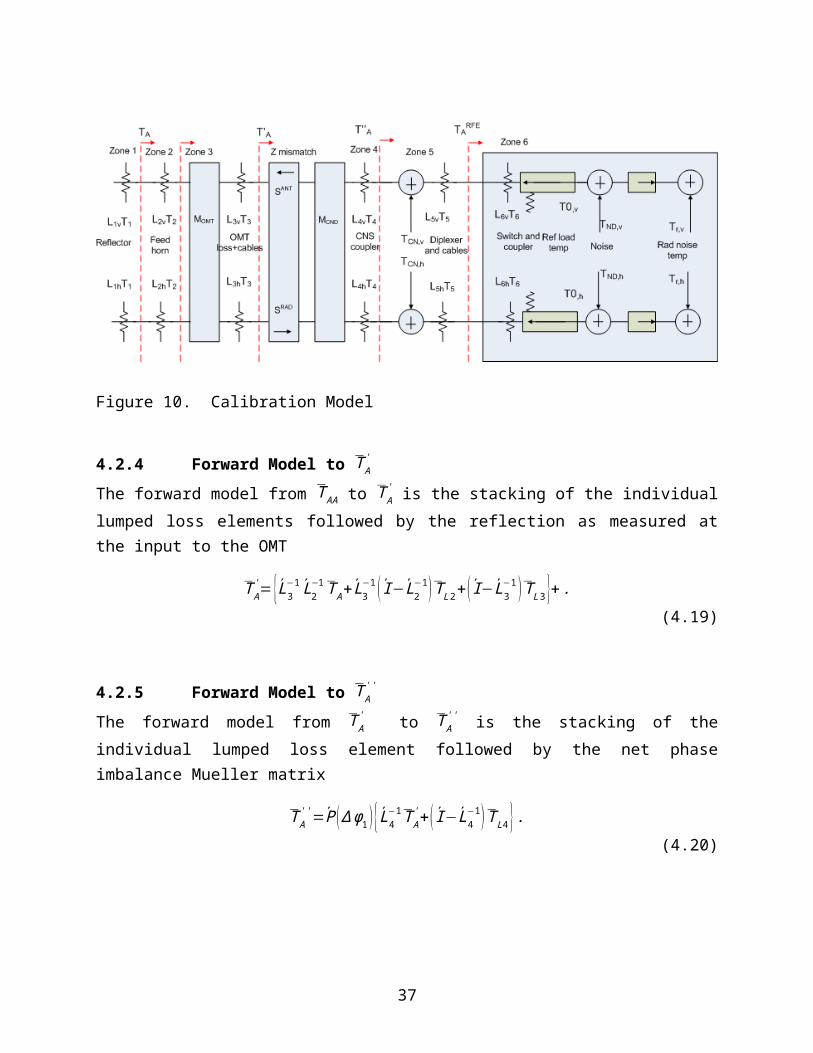
5.1 L1B_TB Algorithm FlowThe baseline algorithm flow for the L1B_TB algorithm processing is illustrated in Error:Reference source not found.

Figure 11. Diagram of the L1A/B radiometer processing

30

5.2 Level 1A ProductThe inputs to the L1A processing are Level 0B files, which are raw radiometer telemetry output with repeats removed, unpacked and parsed. See the Level 0 Software Specification Document, TBD. The processing steps included in the L1A software include unwrapping of instrument CCSDS packets, parsing of radiometer science data into the various radiometric states, storing of time stamps for science data as well as housekeeping telemetry such as temperature, voltage and current monitor points converted to engineering units for each antenna scan. L0 data will be archived but not be made available to the public. It is important to note that the raw science data is preserved in the L1A product allowing re-processing of data. Level 1A and Level 1B are official SMAP data products which will be publicly available. The parameters that are part of the L1A product are defined in the L1A product spreadsheet. See the Radiometer Level 1A Product Specification Document, TBD.

Radiometer data contain science data packets that will be generated once every 4 PRIs. The switching scheme which indicates the radiometer state of a particular science data packet is pre-determined and used to parse the raw science data. The radiometer digital electronics (RDE) box controls when the radiometer reference switch and noise sources are switched during an antenna azimuth scan. This switching can therefore occur every four PRIs or every packet. The switching scheme was optimized for minimum noise and calibration error. See the SMAP Radiometer Calibration Switching Optimization Memo for details of the analysis. When the radiometer is in science mode, the switching sequence for each antenna scan is given in Table 5 and Table 6.

Table 5. Switching sequence for last two footprints of the scan

PKT State CNS1 ANT ON2 ANT3 ANT ON4 ANT5 ANT ON6 ANT7 ANT ON8 ANT9 ANT ON

10 ANT11 ANT ON12 ANT13 ANT ON14 ANT15 ANT ON16 ANT

31

17 ANT ON18 ANT19 ANT ON20 ANT21 ANT ON22 ANT23 ANT ON24 ANT + ND

Table 6. Switching sequence for all other footprints except the last 2 of the scan

PKT State1 ANT2 ANT3 ANT4 ANT5 ANT6 ANT7 ANT8 ANT9 ANT

10 ANT11 ANT12 REF13 ANT14 ANT15 ANT16 ANT17 ANT18 ANT19 ANT20 ANT21 ANT22 ANT23 ANT24 REF + ND

5.3 Geolocation and PointingThe goal of geolocation and pointing with respect to the SMAP radiometer is, in the most basic terms, to determine where the radiometer footprints intersect the Earth’s surface. This is

32

obviously important to be able to interpret all radiometer-derived SMAP data products from L1B_TB and higher. It is also necessary for several of the corrections needed to generate the L1B_TB product itself. For example, the Antenna Pattern Correction requires knowledge of the footprint location in order to estimate contributions to Earth sidelobes, and if a model-based Faraday rotation correction is used, knowledge of the viewing path through the ionosphere will be required, as Faraday rotation is location-dependent. RFI detection and mitigation also can benefit from geolocation knowledge since there are many surface sources with fixed locations. In addition to pointing with respect to the Earth, we also require information on pointing with respect to other celestial targets (the sun and moon, the disk of the Milky Way) in order to quantify direct and reflected signals.

Initially after launch, we will start with

a. the location of the SMAP spacecraft along its orbit (ephemeris); b. spacecraft attitude (pointing); c. orientation of the antenna spin axis; d. the estimated conical-scan nadir cone angle, e. the antenna azimuth angle

to determine the projected point of intersection of the radiometer boresight vector with the WGS84 ellipsoid for each IFOV.

The source of information for (a, b, & e) will be NASA’s Navigation and Ancillary Information Facility’s (NAIF) SPICE software (http://naif.jpl.nasa.gov/naif/spiceconcept.html). The information (a, b, & e) plus timing will be contained in so-called SPICE kernels (files) provided by NAIF based upon output from the SMAP Ground Data System (GDS). Using standard SPICE routines, latitudes and longitudes for each radiometer footprint will be computed. Azimuth, Earth incidence, and polarization rotation angles will also be computed and reported. Along with footprint location, SPICE routines will be used to compute the azimuth and elevation to the sun and moon (if within sight) relative to the spacecraft coordinate frame, antenna frame, and footprint location. Finally, during maneuvers when the antenna main beam does not intersect the Earth’s surface (e.g., during cold sky calibration), the boresight direction will be reported in galactic coordinates.

Items (a-e) are indexed with respect to time. But, different SMAP elements use different clocks (e.g., spacecraft bus clock, radiometer clock, radar clock). We note that in addition to misspecification of any of the items (a-e), misspecification of the time of measurement will also manifest itself as a geolocation error. Therefore, time offsets among these different clocks must be taken into account to avoid geolocation errors.

After SMAP is in a stable orbit, and several orbits of observations have been accumulated (but still during commissioning phase), the initial geolocation estimate will be refined using techniques that have been demonstrated on other spaceborne radiometers to have high sensitivity to small pitch and roll offsets of the antenna spin axis, and small offsets from the assumed nadir cone angle. In other words, previous radiometers have used their TB measurements to correct

33

errors in items (b-d), and we expect SMAP to be similar. This checking and refinement of the radiometer geolocation will continue throughout the mission lifetime, with particular focus following orbit adjustments, calibration maneuvers (e.g. cold space viewing), and any events that have the potential to significantly affect geolocation.

The input variables required correspond directly to the list (a-e) and are listed in Table 7 below. Referring to the L1 processing flow in Figure 11, note that these geolocation input data are combined with the raw radiometer output (counts) data to form the L1A radiometer data product---however, the geolocation process is performed during the generation of the L1B product. The output variables from the geolocation process are also listed in Table 7.

Table 7. Radiometer geolocation variables. All are assumed to be indexed to the time reference for the respective source. Time offsets among these different clocks (e.g., spacecraft bus clock, radiometer clock, radar clock) must be taken into account to avoid geolocation errors from time misspecification errors.

Variable name Unit Valid range Resolution Source I/OSpacecraft location x

SPICE/GDS input

Spacecraft location y

SPICE/GDS Input

Spacecraft location z

SPICE/GDS Input

spacecraft pitch offset

Degree [-180,180] 0.01 s/c attitude control [TBR]

Input

spacecraft Roll offset

Degree [-180,180] 0.01 s/c attitude control [TBR]

input

spacecraft yaw offset

Degree [-180,180] 0.01 s/c attitude control [TBR]

Input

antenna spin axis pitch offset wrt s/c nadir

Degree [-180,180] 0.01 Pre-launch measurement & calc

Input

antenna spin axis roll offset wrt s/c nadir

Degree [-180,180] 0.01 Pre-launch measurement & calc

Input

Antenna nadir cone angle

Degree [0,90] 0.01 [TBR] input

antenna spin azimuth angle

Degree [0,360] 0.01 [TBR] ICE [TBR] Input

OR time index pulse

Second [TBR]

0.01 [TBR] ICE [TBR] Input

34

WITH spin rpm 1/minute [0-15] 0.01 [TBR] ICE [TBR] InputClock offset radiometer to bus

Second [TBR]

[-1,1] 1E-5 [TBR] Pre-launch measurement

Input

Clock offset radiometer to ICE [TBR]

Second [TBR]

[-1,1] 1E-5 [TBR] Pre-launch measurement

Input

Clock offset radiometer to orbit ephemeris

Second [TBR]

[-1,1] 1E-5 [TBR] Pre-launch measurement

Input

Radiometer packet index

count [1-24] 1 Radiometer controller [TBR]

input

Radiometer IFOV azimuth angle wrt subsatellite track

Degree [0,360] 0.01 [TBR] output

Radiometer IFOV boresight latitude

Degree [-90,90] 0.1 output

Radiometer IFOV boresight longitude

Degree [-180,180] 0.1 output

Radiometer IFOV boresight altitude

km [same as range of WGS84 altitude]

0.1 [TBR] output

Radiometer IFOV boresight time index

Second [TBR]

output

Radiometer EFOV boresight latitude

Degree [-90,90] 0.1 output

Radiometer EFOV boresight longitude

Degree [-180,180] 0.1 output

Radiometer EIA wrt WGS84

Degree [0,90] 0.1 Output

Radiometer geometric polarization rotation

Degree [0,90] 0.1 Output

Sun azimuth in Degree [-180,180] 0.1 Output

35

antenna coord frameSun elevation in antenna coord frame

Degree [-90,90] 0.1 output

Moon azimuth in antenna coord frame

Degree [-180,180] 0.1 Output

Moon elevation in antenna coord frame

Degree [-90,90] 0.1 output

Boresight off Earth flag

binary output

s/c maneuver flag

binary GDS [TBC] input

Because radiometer geolocation is intimately connected with other steps in the L1B processing flow. For example, Faraday rotation correction and Antenna Pattern Correction, it makes sense to try and integrate its computation with the computation of these other steps.

5.3.1 Long-term refinement of radiometer geolocationAs mentioned above, other conical-scan radiometers have demonstrated techniques with high sensitivity to small pitch and roll offsets of the antenna spin axis, and small offsets from the assumed nadir cone angle. SMAP will also use these techniques to refine the geolocation and pointing solutions beyond what can be computed solely from the SPICE-based information.

5.3.1.1 Correction of IFOV lat/lon using coastline crossingsThe large Tb contrast at land-water boundaries provides high-sensitivity locations for checking and refining the precise location of the IFOV boresight. For example, if the sub-satellite track crosses perpendicular to a shoreline, the TB versus time response at the swath edges is given by the convolution of a step function with the antenna pattern with the time axis rescaled into distance units. The midpoint of the TB change occurs right when the boresight intersects the coastline. Sub-pixel precision is achievable. The scanning SMAP beam will cross coastlines frequently, providing frequent opportunities to perform this check.

5.3.1.2 Correction of pitch & roll offset with 360-deg scan With SMAP’s 360 degree conical view, we can exploit circular symmetry to check for offsets in the pitch and roll attitude of the combined spacecraft-antenna spin axis system. This technique takes the TBs around the 360 degree scan under uniform ocean conditions, and looks for deviations from what should be a constant TB. It will require sea surface state forecast ancillary

36

information to identify appropriate 1000 km wide (to match SMAP swath width) ocean areas and weather conditions (e.g., no precipitation). The symmetry of TH, TV, T3, and T4 will each be checked.

5.3.2 Radiometer geolocation and radar geolocation compatibilityThe boresight vectors of the radiometer and radar are not necessarily exactly the same, although the difference is expected to be insignificant [TBC] versus the radiometer geolocation accuracy requirement.

Although the SMAP radar is expected to achieve higher-precision geolocation/pointing knowledge than the radiometer, we intentionally do not rely on radar geolocation information in order to generate the L1B_TB product. The 12-hour latency requirement on the L1B_TB product does not leave a lot of time to wait for the radar geolocation solution to be computed, and then to perform all the L1B processing steps. This is the lowest-risk approach to ensure the fundamental L1B_TB science product is independent of any possible delays in radar data downlink or processing, or the worst-case scenario of no radar.

The L1B_TB geolocation described in this section is compatible with higher-level SMAP data products such as L2_SM_AP that involve combined passive and active retrievals.

5.4 Nonlinearity CorrectionFor each of the V and H channels, nonlinearity correction is performed on the sum of the second moment of the in-phase and second moment of the quadrature signal components. See Figure12. Correction coefficients and their temperature dependencies will be measured during pre-launch calibration testing at GSFC. The correction algorithm operates directly on the uncalibrated detector count values C from the radiometer. The linearized count value Clin is expanded into a polynomial of raw counts C:

C lin=C +c2C2+c3C3

(5.27)

The expansion coefficients c2 and c3 are expanded as functions of physical temperature:c2=¿c2,0+c2,1 ΔT+c2,2 ΔT 2¿

(5.28)

c3=¿c3,0+c3,1 ΔT+c3,2 ΔT 2¿

(5.29)

where∆ T=T p , 0−T ref 0

(5.30)

37

Nonlin correction

Nonlin correction

CalibrationIHIV+QHQV T33

CalibrationIHQV-IVQH T44

is the deviation of the detector temperature Tp,0 from a reference temperature Tref0.

5.5 Calibration Coefficients ComputationPrior to radiometric calibration, calibration coefficients are computed and stored in the L1B_TB product. Instrument parameter files containing noise diode and front end loss coefficients are used to compute noise diode and front end losses. See the calibration model in Figure 10. These losses are used in subsequent equations in the TA calibration algorithm. These instrument parameter files will be made time dependent which takes into account component drifts.

5.6 Radiometric CalibrationRadiometric calibration will be performed on each radiometer channel in both the time and frequency domains. The second moment, which is proportional to the output power of the radiometer, will be used to produce TA and TB. For each of the V and H channels, the second moment of the in-phase and second moment of the quadrature signal components are summed to produce the baseband signals which in turn are calibrated to obtain TAH and TAV. The second moment values to be used in radiometric calibration will be the linearized counts as described in Section 5.4. The 3rd and 4th Stokes parameters will also be calibrated for both the fullband and each of the 16 subbands. See Figure 12.

Figure 12. Calibration of radiometer counts

ANT, REF, REF+NDCounts

H Calibration TAHM2I+M2Q

V Calibration TAVM2I+M2Q

38

5.6.1 Horizontal and Vertical ChannelsEstimation of the antenna temperature T A is performed using internal calibration references

referred to the input of the RFE (the T ARFE plane), and then the antenna temperature vector is

propagated back to the antenna feedhorn aperture (the T A plane) with necessary corrections including losses, physical temperatures, reflections and phase offsets. See Figure 10.

Given a linear radiometer approximation, the calibration equation for the horizontal and vertical channels (referred to the RFE input) is

T A , pRFE=T ND, p

RFE ( C A , p−C ref , p

C ref + ND , p−Cref , p)+T ref , p

(5.31)

where subscript p = V, H denotes polarization channel; C A is the radiometer output with the Dicke switch turned towards the antenna and no noise diodes active, C ref is the radiometer output with the Dicke switch turned towards the reference load, and C ref + ND is the radiometer output with the Dicke switch turned towards the reference load and the noise diode activated. T ref is the antenna temperature of the reference load and it is equal to its physical temperature. Noise diode antenna temperature T ND

RFE is a function of RFE physical temperature:

T ND , pRFE (T sensor )=T ND , p

RFE (T 0 )+c ND, p (T sensor−T 0 )(5.32)

where T 0 is a reference temperature at which T ND , pRFE (T 0 ) was measured. The temperature T sensor is

obtained from the temperature sensor measurement and c ND, p is the fractional temperature coefficient of the noise diode.

Once the antenna temperature at the RFE input is found, the antenna temperature is propagated backward to the antenna feedhorn aperture. At the CNS coupler input without impedance-mismatching correction, the antenna temperature is given by

T A , pCP =L4 , p L5 , p T A , p

RFE− ( L4 , p−1 ) T L4 , p−L4 , p ( L5 , p−1 )T L 5 , p

(5.33)

After impedance-mismatching correction, the antenna temperature at the CNS coupler input is give by

(5.34)

39

Then the calibrated antenna temperature at the feedhorn input is given by

T A , p=L2 , p L3 , p−( L2 , p−1 ) T L2 , p−L2 , p ( L3 , p−1 )T L3 , p

(5.35)

In Equations (5.33) and (5.35), all of the losses are temperature dependent and they are modeled as linear functions of their temperature:

Lx (T Lx )=Lx (T Lx ,0 )+cx ( T Lx−T Lx , 0 )(5.36)

where T Lx , 0 (x = 2,3,4,5) is a reference temperature at which Lx(T Lx ,0 ) was measured. The

temperature T Lx is obtained from temperature sensor measurement and c x is the fractional temperature coefficient of the loss. Subscript ‘p’ is ignored in this equation.

5.6.2 Third and Fourth Stokes ParametersThe 3rd and 4th Stokes channel characteristics can be calibrated using the noise diode and the reference load as well. With and without the noise diode coupled into the receiver when the Dicke switch is switched to the reference load, the radiometer responses are given by

[Cref , 3

Cref , 4 ]=[G33 G34

G43 G44 ][Tref , 3RFE

Tref , 4RFE ]+O34

=O34(5.37)

[Cref +ND , 3

Cref +ND , 4 ]=[G33 G34

G43 G44 ][T ref , 3RFE +T ND , 3

RFE

T ref , 4RFE +T ND, 4

RFE ]+O34

=[G33 G34

G43 G44 ] [T ND, 3RFE

T ND, 4RFE ]+O34

(5.38)

where T ND , xRFE

(x = 3,4) is the 3rd/4th antenna temperature of the noise diode referenced to the RFE

input. T ref , xRFE

(x = 3,4) is the 3rd/4th antenna temperature of the reference loads and they are equal

to zero. O34 is offset vector corresponding zero input response. The difference between Equations (5.38) and (5.38) gives

40

[Cref +ND , 3−C ref ,3

C ref + ND, 4−C ref , 4 ]=[G33 G34

G43 G44 ] [T ND , 3RFE

T ND ,4RFE ]

(5.39)

If the radiometer channel phase imbalance is stable or if it can be measured during pre-launch calibration, then for a radiometer with digital back end, the gain matrix in Equation (5.37) for the 3rd and 4th Stokes channel can be represented by

[G33 G34

G43 G44 ]=G3∧4 [cos ( Δθ ) sin ( Δθ )−sin ( Δθ ) cos ( Δθ ) ]

(5.40)

where G3∧4 is the gain magnitude of 3rd/4th Stokes channel; Δθ is the channel phase imbalance counted from calibration reference plane to radiometer output.

Let

[T ND, 3RFE

T ND , 4RFE ]=T ND , 3∧4

RFE [cos (Δϑ ND )sin ( Δϑ ND ) ]

(5.41)

where Δϑ ND is the noise diode channel phase imbalance referenced to the RFE input. T ND ,3∧4RFE

is the antenna temperatureof the noise diode 3rd/4th Stokes parameters referenced to the RFE input.

Then the gain magnitude of 3rd/4th Stokes channel is estimated by

G3∧4=(Cref + ND,3−Cref ,3 ) cos ( Δθ−Δϑ ND )−( Cref +ND , 4−C ref ,4 )sin (Δθ−Δϑ ND )

T ND ,3∧4RFE

(5.42)

Assume that impedance-mismatching status is unchanged when the Dicke switch works between the antenna and the reference load. When the Dicke switch turns toward the antenna, the radiometer output response is given by

[CA ,3

C A , 4 ]=[G33 G34

G43 G44 ][T A , 3RFE

T A , 4RFE ]+O34

(5.43)

Then the estimated 3rd and 4th Stokes parameters are given by

41

[ T A , 3RFE

T A ,4RFE ]=[C A , 3cos ( Δθ )−C A , 4sin ( Δθ )

C A , 3sin ( Δθ )+CA ,4 cos ( Δθ ) ]−[C ref , 3cos ( Δθ )−C ref , 4 c sin ( Δθ )C ref , 3 c sin ( Δθ )+C ref , 4cos ( Δθ ) ]

G3∧4

(5.44)

The 3rd and 4th Stokes parameters at the feedhorn input can be derived by

[ T A ,3

T A ,4 ]=√∏m=2

5

Lm, v∏n=2

5

Ln ,h¯P−1( Δψ ) ¯M 3∧4

−1 [ T A , 3RFE

T A ,4RFE ]

(5.45)

where

¯P( Δψ )=[cos ( Δψ ) sin ( Δψ )−sin ( Δψ ) cos ( Δψ ) ]

(5.46)

¯M 3∧4=[Re Λv Λh¿ −Im Λv Λh

¿

Im Λv Λh¿ Re Λv Λh

¿ ](5.47)

where Δψ is the phase imbalance between V and H channels counted from feedhorn to the RFE input.

42

5.7 Radio Frequency Interference (RFI)SMAP’s radiometer passband lies within the 1400-1427 MHz Earth Exploration Satellite Service (EESS) passive frequency allocation. Both unauthorized in-band transmitters as well as out-of-band emissions from transmitters operating at frequencies adjacent to this allocated spectrum have been documented as sources of radio frequency interference to the L-band radiometers on SMOS and on Aquarius. This is a serious issue that is expected to be present during the SMAP mission lifetime and SMAP will be the first spaceborne radiometer to fly a dedicated subsystem to enable detection and mitigation of RFI.

The radiometer instrument architecture provides science data with time-frequency diversity enabling the use of multiple RFI detection methods. The RFI detection and mitigation algorithms are part of the L1B processing which will be performed in ground processing. See Figure 11. Previous airborne and ground based experiments were assessed to predict the RFI environment SMAP will be facing. SMAPVEX08 was one such campaign which provided a comprehensive database of RFI present in the United States [Park et. al 2011]. Since a number of RFI detection methods were demonstrated during these campaigns, a combination of these methods will be incorporated into the RFI detection algorithm for SMAP. A pulse detection method as well as cross frequency and kurtosis detection methods will be employed. The third and fourth Stokes parameters are also included with the primary purpose of RFI detection. A maximum probability of detection algorithm will be used to combine the outputs of each detection method. Data indicated as RFI within a footprint will be removed and the rest averaged to produce the antenna temperature, TA, for that footprint. RFI detection algorithms (except the kurtosis algorithm which operates on moments) will be performed on calibrated data or TA referenced to the feedhorn.

5.7.1 RFI SourcesSatellite data sets such as that from SMOS and Aquarius are of limited utility in classifying

source types i.e. pulsed, narrowband, wideband etc. Airborne data sets can provide more details on this type of information. The sources of L-band RFI are critical to SMAP. The RFI model described below takes into consideration two main types of RFI: pulsed and CW. They represent the main sources of RFI at L-band known from literature, the spectrum engineering community and airborne field campaigns. The airborne campaign, SMAPVEX08 showed most US RFI to be either pulsed or narrowband (CW) type with a wideband example occurring only once in the campaign which comprised over 100 flight hours. Wideband continuous sources at low levels which occupy ~4 MHz or more are a concern since they are difficult to detect using either frequency or time based algorithms. These broadband sources can potentially be detected by polarimetric and kurtosis detection. Polarimetric and kurtosis detection of wideband sources will be evaluated using test data since these examples are lacking from airborne data and indeterminate from existing satellite data.

RFI simulations have been performed for pulsed (e.g., radar) and CW-type (e.g., spurious emission) RFI sources to determine algorithm performance of various detection methods. It is

43

shown that the detection strategies described below can effectively mitigate these main sources of L-band RFI. Since the RFI environment is uncertain, other RFI types will be studied to evaluate algorithm performance. The algorithm response to signals such as QPSK, OFDM, etc. will be studied via test rather than simulations which were previously done for pulsed and CW sources.

5.8 RFI Detection Algorithm Theory

5.8.1 Pulse or Time Domain DetectionThe pulse or time domain detection algorithm searches in the time domain for increased levels of observed antenna temperatures above that produced by geophysical properties. The algorithm is also referred to as asynchronous pulse blanking since no periodic properties of the RFI are assumed. This detection method is best suited to detect RFI with large amplitudes and short duration times or duty cycles, properties inherent of the main RFI sources observed at L-band (air surveillance radars) also known as pulsed RFI. These radar pulses or pulsed RFI below the 1400 MHz passive frequency allocation, range from 2 to 400 µs in length and occur 1-75 ms apart [Ellingson, 2003]. In order to detect these pulses, the standard asynchronous pulse blanking algorithm calculates a running mean and standard deviation used to threshold data. The robust mean and standard deviation can be estimated from each time window without the largest N% of samples. If a time domain sample is a certain number of standard deviations above the mean, the algorithm flags it as RFI. The number of standard deviations used to threshold data determines the false alarm rate or FAR. The robust estimator, however, removes outliers in the noise distribution which tends to artificially reduce the standard deviation and increases the FAR. This can be overcome by determining the standard deviation of the system temperature a priori since it does not vary significantly with time. The adaptive mean calculation is still necessary to account for variability in the scene. Previous pulse blanking algorithms also flag and blank a preset number of samples before and after each detection to include any multipath components that may be associated with the detected pulses [Niamsuwan et. al, 2005].

5.8.2 Cross Frequency DetectionThe cross frequency detection algorithm is similar to the pulse detection algorithm except that it searches for increased levels of antenna temperatures which are recorded in multiple frequency channels. This detection algorithm performs best on narrow band sources whose frequency resolution is matched to that of the measurement; however, no RFI properties are assumed in the algorithm. The algorithm consists of thresholding in the frequency domain. A robust mean and standard deviation are estimated for each time subsample without the largest N channels and like the pulse detector, antenna temperatures a certain number of standard deviations above the mean are flagged as corrupted with the threshold level determining the FAR. This detection method

44

has been shown to be more sensitive to CW RFI while the pulse and kurtosis detectors are more insensitive to this kind of RFI [Güner et. al, 2010].

5.8.3 Kurtosis DetectionNatural thermal emission incident on a space-borne radiometer and the thermal noise generated by the receiver hardware itself are both random in nature. The kurtosis algorithm makes use of the randomness of the incoming signal to detect RFI. Thermally generated radiometric sources have an amplitude probability distribution function that is Gaussian in nature, whereas man-made RFI sources tend to have a non-Gaussian distribution [Ruf et al., 2006]. The kurtosis algorithm measures the deviation from normality of the incoming radiometric source to detect the presence of interfering sources.

The kurtosis detection algorithm measures higher order central moments of the incoming signal than the 2nd central moment measured by a square-law detector in a total power radiometer. The nth central moment of a signal is given by

mn=⟨ ( x (t )−⟨ x ( t )⟩)n⟩(5.48)

where x(t) is the pre-detection voltage and <⋅> represents the expectation of the measured signal. The kurtosis is the ratio of the 4th central moment to the square of the 2nd central moment,

or

κ=m4

m22

(5.49)

The kurtosis equals three when the incoming signal is purely Gaussian distributed and it in most cases deviates from three if there is a non-normal (typically man-made) interfering source present. The kurtosis statistic is independent of the 2nd central moment of the signal, i.e., the kurtosis value is not affected by natural variations in the antenna temperature of the scene being observed.

The kurtosis estimate itself behaves like a random variable since it is generally calculated from a finite sample set [Kenney and Keeping, 1962]. Estimates of the kurtosis have a standard deviation associated with them, and there is a corresponding kurtosis threshold for detecting RFI. If the sample size is sufficiently large (> N = 50,000 [DeRoo et al., 2007]), the kurtosis estimate exhibits a normal distribution.

5.8.4 Polarimetric detectionNatural scenes have highly variable horizontal and vertical brightness temperatures but the 3rd

and 4th Stokes parameters are nearly always zero unless RFI is present [Pardé et. al, 2011].

45

SMAP has included the 3rd and 4th Stokes parameters for both the fullband and each of the 16 subbands. RFI can be detected by looking for unusually large variations in the 3 rd and 4th Stokes parameters.

5.8.5 RFI ModelAir-traffic control radars and early warning radars are expected to be sources of RFI at L-Band [Piepmeier et al., 2006]. A general expression is considered as the model for RFI which provides for the possibility of multiple pulsed-sinusoidal sources. It is given by

N

i iiii w

ttrecttfAtntx1

02cos

(5.50)

Tt ,0

where n(t)~N(0,2) is normally distributed with zero mean and standard deviation . A is the amplitude of the RFI source, f is the frequency, is the phase shift, t0 represents the center of the ON pulse of the duty-cycle, w is the width of the pulse and T is the integration period. The ratio (d=w/T) represents the duty-cycle of the RFI source. f is assumed to be uniformly distributed between [0, B] where B is the bandwidth of the radiometer. and t0 are assumed to be uniformly distributed over [0, 2] and [0,T] respectively. N is the total number of RFI sources.

The model described in Equation (5.50) has two undetermined random variables associated with it: the amplitude A and the duty cycle d. Within an antenna footprint it is expected that the various RFI sources would have a variety of power levels. In addition, the side lobes will see an RFI source differently than the main lobe of an antenna does. As a result, A is modeled as a random variable. In order to obtain characteristic data of a typical RFI amplitude distribution, the SMAPVEX08 campaign was used. Figure 13 shows the distribution of RFI power observed during the campaign, specifically the percent of total RFI present within 0.5 K bins from 0 to 20 K. The distribution of RFI power is seen to be exponential in nature, consisting primarily of low-power RFI with a much lower probability of high-power sources. Assuming the SMAPVEX08 data are representative of RFI in general, the amplitude probability density function (pdf) can be expressed as

f ( A )=1υ

exp (−A /υ )

(5.51)

where, f() represents the pdf, A is the amplitude random variable of RFI, and is the mean of the exponential pdf. For simulation purposes, the exponential mean is scaled to match the total

46

power contribution (sum of the distribution) between scenarios with different numbers of sources.

Figure 13. Normalized distribution of RFI brightness temperature observed during the SMAPVEX08 campaign

It is assumed that multiple RFI sources within an antenna footprint will generally have different duty cycles from one other. Relative occurrence of RFI with a pulsed or CW duty cycle can be characterized in a data set like that of the SMAPVEX08 campaign by noting whether the value of the kurtosis was above or below 3.

In general at L-band, RFI is mostly pulsed-type in nature as noted from the SMAPVEX08 flight campaign and similar results in Misra et. al (2009) and Park et. al (2011). Communication signals exhibit CW behavior, or have high duty-cycle. Thus we consider a bimodal pdf with respect to duty cycle, where the low-duty cycle region is approximated by a Rayleigh distribution and the high duty cycle region is approximated by an exponential distribution, or

f (d )= p ( dbd

2 exp (− d2

2bd2 ))+ (1− p )( 1

υdexp(−1−d

υd ))(5.52)

47

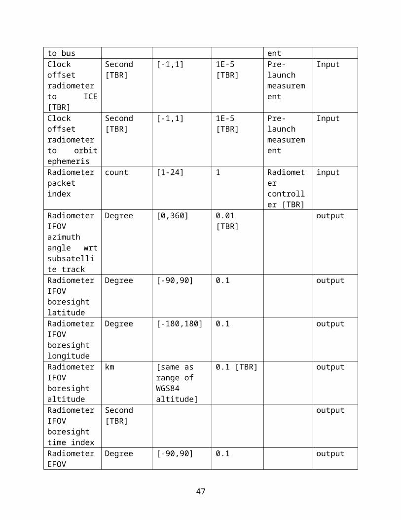
where, f() is the probability density function, d is the duty-cycle (pulse width) (considered a random variable), p is the fraction of low duty-cycle sources, 1-d is the mean of the exponential pdf and bd is the mode of the pdf. For simulation purposes, d is assumed to be ~0.1 and bd is assumed to be ~0.05. Both values are variable parameters that can be changed to assess the performance of detection algorithms. The Rayleigh distribution approximates a mostly low duty-cycle signal, whereas the decaying exponential pdf approximates signals around 100% duty-cycle trailing off towards 50%. The fraction p is a variable parameter that controls the amount of low to high duty-cycle sources within a single footprint. Figure 14 is an example of a duty-cycle pdf with an equal number of high and low duty-cycle sources.

Figure 14. An individual realization of the bimodal pdf applied for duty-cycle of individual RFI sources. The fraction of low duty-cycle to high duty-cycle is a variable parameter with the above plot indicating 50% of sources with low duty cycle.

The probability density of Equation (5.50) is given by a derivation. See Misra et. al (2012),

N

iiii

u

duAJdeFtf1

021 1

22

(5.53)

48

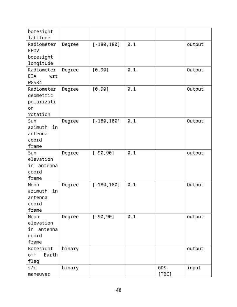
where J0 is a Bessel function of the zeroth order, Ai is the amplitude of the ith RFI source, di is the duty-cycle of the ith RFI source, is the standard deviation of a normally distributed function and F-1[…] represents the inverse Fourier transform operation with respect to u.

Figure 15 shows two pdf’s, one of a Gaussian signal corrupted by a single RFI source and the other corrupted by multi-source RFI. Note that these distributions will in general depend on various parameters such as mean power and duty-cycle fraction. Due to central limit theorem conditions, the pdf of a multi-source corrupted thermal signal will approach a Gaussian distribution, similar to the uncorrupted original signal, as the number of sources increases. This property is expected to impact the performance of the kurtosis detection algorithm with regard to detectability of RFI.

Figure 15. Probability density function of RFI with thermal noise. The blue curve is for a single RFI source, and the green is for multiple sources, i.e. 50 sources, all of which have low duty cycle. The relative RFI power of the different types of RFI sources is approximately 10 times the thermal noise.

5.8.6 FAR and PD of Detection Algorithms The two RFI parameters that vary in the RFI model presented in the previous section are its duty cycle and amplitude (or power). These parameters significantly affect the detection performance. The behavior of both detection algorithms in the presence of pulsed-sinusoidal RFI has been extensively analyzed previously [De Roo et al., 2007; Johnson and Potter, 2009]. The kurtosis detection algorithm is extremely sensitive at low duty cycles. When the pulsed-

49

sinusoidal RFI has a 50% duty-cycle, the detection algorithm has a blind-spot since the kurtosis value is three. This may not seem to be a problem since most radar signals have a very low duty-cycle, but can become important when time sub-sampling is utilized.

For equal thresholds above and below the kurtosis mean, the FAR of the kurtosis detection algorithm is given by [De Roo et al., 2007]

Qκ ( z )=(1−erf ( z√2 ))

(5.54)

where z is the normalized magnitude of the standard deviation of the kurtosis (i.e. the threshold is set at 3 +/- zR0, where R0 is the standard deviation of RFI free kurtosis), beyond which a sample is flagged as being corrupted by RFI.

In practical implementations of the detection algorithm the incoming signal is divided into temporal sub-samples, or spectral sub-samples, or both before calculating the kurtosis statistic [Ruf et al., 2006]. If any sub-sample is flagged, then it is discarded. In order to compare the kurtosis algorithm with other detection algorithms, an entire radiometer integration period is assumed to be corrupted by RFI if any single sub-sample is flagged. Equation (5.54) can be rewritten to calculate the FAR for detection of the whole temporal/spectral grid of sub-samples within the integration period, as given by

QκnoRFI ( z )=1−(1−Qκ ( z ) )XR

(5.55)

where z is the normalized standard deviation magnitude of the kurtosis (i.e. the threshold is set at zR0, where R0 is the standard deviation of RFI free kurtosis), R is the number of temporal sub-sampling periods within an entire integration period, and X is the number of spectral sub-bands.

To simplify the analysis, pulsed-sinusoidal RFI is assumed to be located fully within a single frequency channel of the kurtosis algorithm when spectral sub-banding is used; this improves detection performance since the RFI signal-to-noise ratio is larger in this channel. Temporal sub-sampling also improves detection performance since it reduces the interval over which the RFI power is averaged and hence increases the relative RFI power measured. The analysis allows an RFI pulse to be spread over multiple temporal sub-samples if the sub-sampling period is smaller than the RFI pulse-width. Sub-sampling and sub-banding reduce the number of independent samples used to calculate kurtosis, as a result of which slight skewness is introduced to the normal distribution of the kurtosis statistic. However, this skewness is not modeled in what follows. The probability of detection (PD) for the kurtosis algorithm for a single sub-sampling period and a single frequency channel can be calculated if the duty-cycle and power of the RFI signal are known. The PD was given by [De Roo et al., 2007] and is repeated here

50

Qκpulsed−sin RFI ( z )=(1∓erf ( R th−R ( S , d )

√2 σ R (S , d ) ))(5.56)

where S is the relative power of the pulsed-sinusoidal RFI to the thermal signal, d is the duty-

cycle of the RFI, R and σ R are the mean and standard deviation of kurtosis for a pulsed-sinusoidal RFI with relative power S and duty cycle d given in [De Roo et al., 2007],Rth=3±zσ RO is the kurtosis threshold, and σ R 0 is the standard deviation of RFI free kurtosis. As mentioned above, an integration sample is divided into finer temporal and spectral resolution sub-samples, thus creating a grid. In order to detect RFI, the kurtosis with the maximum deviation from 3 within a temporal and spectral sub-sampling grid is measured. If that particular

kurtosis sub-sample is above 3+zσ RO , or below 3−zσ RO , then the grid is considered to be corrupted by RFI, and hence the whole integration sample is flagged as being corrupted by RFI. Thus, the final probability of detection is obtained by taking the maximum kurtosis deviation among the set of frequency and time resolved kurtosis values.

The pulse detection algorithm performs best when the sub-sample integration time is matched to the pulse-width of the RFI. The performance degrades as that sub-sampling time increases relative to the pulse-width. For time intervals containing RFI pulses, the power in the incoming signal is a non-central Chi-square random variable with the non-centrality parameter determined by the power and duty cycle of the RFI. The PD of the pulse detection algorithm can be calculated using the right-tail cdf of a non-central chi-squared random variable given in [Johnson and Potter, 2009] with non-centrality parameter

λ=∑n=m

m+d

A2 sin2 (2 πf o n )(5.57)

where A is the amplitude of the pulsed-sinusoid signal with frequency fo and d is the pulse-width of the RFI, determining the duty cycle.

5.8.7 Area Under Curve (AUC) ParameterizationThe receiver operating characteristic (ROC) of any detection algorithm is a graphical plot of the probability of detection (fraction of true positives) versus the false alarm rate (fraction of false positives). Figure 16 gives the ROC curves of the kurtosis and pulse detection algorithms for RFI with M=240,000, N=200, d=800 (a duty cycle of 0.33% relative to the total integration period) and an average power level of 0.5 NET. In Figure 16 [Misra et. al 2009], two versions of the ROC curve for the kurtosis algorithm are shown; one curve represents the full-band kurtosis with no temporal sub-sampling and the other assumes 16 spectral sub-bands are available and the data are sub-sampled at a rate that is a quarter of the total integration period.

51

The third curve indicates the pulse detection algorithm, with the total integration period divided into 1200 sub-sampling periods. In general, better detection algorithms correspond to a ROC curve that is closer to the upper left corner of the PD vs. FAR space.

0 0.2 0.4 0.6 0.8 10

0.1

0.2

0.3

0.4

0.5

0.6

0.7

0.8

0.9

1ROC curves

False Alarm Rate

Prob

abili

ty o

f Det

ectio

n

Kurtosis Detection Algorithm - FullbandPulse Detection AlgorithmKurtosis Detection Algorithm - Sub-sampled

Figure 16: Plot of the ROC curves for three RFI detection schemes (Pulse-detection algorithm, Fullband kurtosis detection algorithm, Sub-sampled kurtosis algorithm) for a 0.33% duty-cycle pulsed-sinusoid RFI with a 0.5 NET power level.

In order to estimate the relative performance of the detection algorithms under various conditions, the normalized area under the ROC curve (AUC) is used as a performance metric. An ROC curve that runs diagonally across the PD vs. FAR space with a positive slope represents the case of a detector without a priori information, i.e. a “50/50” guess as to whether RFI is present or not. The AUC parameter is scaled so that such a case has a performance metric of 0, whereas an AUC of 1 indicates an ideal detector, with zero probability of false alarms or missed detections. In Figure 16, the full-band kurtosis algorithm (with a 0.33% duty cycle and 0.5 NET power level) has an AUC of 0.0012, whereas the sub-band kurtosis algorithm has an AUC of 0.85 and the pulse detection algorithm has an AUC of 0.69. These values suggest that the sub-band kurtosis as configured here is the best algorithm for this particular type of RFI. It

52

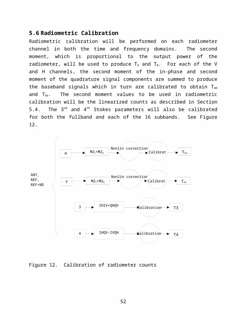
should be noted that even though one algorithm performs better than the other, the performance might still not be optimal with the current configuration for this type of RFI.

5.9 Baseline Detection Algorithms

5.9.1 Time domain RFI detectionA conventional pulse detection method will be performed on the fullband antenna temperatures at the antenna TA for both the V and H polarization to detect RFI in the time domain. Data within a pulse repetition interval, PRI, are integrated for ~300 µs to produce radiometer science data. Thresholding occurs within a footprint which contains 44 PRIs of antenna look data. RFI detection occurs when

T A ( t )−m(t)≥ β td σ td(t )(5.58)

where m(t) is the mean of a pre-determined window without the largest 10% of samples to avoid biasing from RFI and σ(t) is the standard deviation of those samples. This window contains samples from the footprint under observation as well as samples before and after. An example simulation of time domain RFI detection and mitigation is shown in Figure 17. The NEΔT of the radiometer can be used in place of σtd(t) and will be determined in pre-launch calibration. Samples that are βtd standard deviations above the mean are flagged as RFI. Pulse detection will be performed on data with the highest rate to best resolve pulsed RFI; however, the algorithm will also be performed on time domain data that have been integrated at various time intervals, a process which may resolve pulses with different duty cycles. The numbers of samples to be integrated within a footprint before detection are 1, 2 and 4.

The choice of βtd determines where the time domain detection algorithm will operate on the receiver operating curve (ROC), thus establishing its false alarm rate (FAR) and probability of detection (PD). Similar threshold values exist for the other detection algorithms described below. With each detection algorithm, the value of can be varied geographically, via a lookup table, with 1x1 degree resolution in latitude and longitude, to account for variations in the likelihood and type of RFI. A uniform pre-launch value for β will be set so that the FAR causes an increase in the effective NEDT of the footprint average of 5% when no RFI is present. This corresponds to a FAR of 9.3%. It is expected that the value used for will be revisited after launch, once the actual RFI environment has been characterized. For example, it may be prudent to increase the FAR in geographical regions subject to persistent RFI in order to improve the PD, since widespread low-level RFI will be more likely. This type of geographic adjustment to the RFI detection threshold is currently underway for the Aquarius mission.

53

0 5 10 15 20 25250

300

350

400

450

time (ms)

high

-rate

TA

(K)

0 5 10 15 20 25250

300

350

400

450

time (ms)

Figure 17. Left panel shows detected RFI and in the right panel, the RFI is removed. The data were modeled using ~250 µs integration time with an average of 1 K of pulsed RFI.

5.9.2 Cross-frequency RFI detectionSMAP’s instrument architecture provides time-frequency data to enable RFI detection in the frequency domain. The inputs to the cross frequency algorithm are subband antenna temperatures, TA for both the V and H polarization. The passband is divided into 16 sub-bands and the science data contain samples which are integrated every 4 consecutive PRIs (~1.2 ms) for each sub-band. The cross frequency algorithm operates on a single time sub-sample of 16 frequency sub-bands at a time. For each time sub-sample, RFI detection occurs similarly to Equation (5.29). For a given integration period, the average of 16-N channels with the smallest TA is used to estimate the mean and standard deviation of the frequency sub-bands. As in the pulse detection algorithm, an adaptive standard deviation is not necessary and can be determined in pre-launch calibration. A value of N=2 will be used as the change in the mean is less than 1 K if RFI is absent. Any channel which contains TA that are βcf standard deviations above the mean is flagged as corrupted and then removed. Subbands adjacent to those flagged as containing RFI are also flagged as corrupted and removed. It is determined that as many as half of the subbands can be removed and the rest averaged will still meet the NEΔT requirement. As with the pulse detection method, βcf determines the FAR. The remaining samples are then averaged to form a footprint. The cross frequency algorithm will be performed on samples at different integration times. The numbers of time sub-samples to be integrated within a footprint before cross frequency detection are 1 and 11 (see Figure 18).

54

Channel #

Tim

e (m

s) o

r Pac

ket #

1 4 8 12 16

5

10

15

20

25 250

300

350

400

450

500

Channel #

Tim

e (m

s) o

r Pac

ket #

1 4 8 12 16

5

10

15

20

25 250

300

350

400

450

500

Figure 18: RFI detected and removed by cross frequency. The data were modeled using ~1 ms integration time with an average of 1 K of pulsed RFI.

5.9.3 Kurtosis DetectionThe kurtosis detection algorithm will detect the presence of RFI with the SMAP radiometer using the kurtosis statistic. The kurtosis statistic is computed from the first four raw moments of the radiometer signal. The formal definition for the kurtosis of a random variable, x, is given by

K=⟨( x−⟨ x ⟩)4 ⟩

⟨ ( x−⟨ x⟩ )2 ⟩2

(5.59)

where <> denotes the expectation operator. It is the fourth central moment of x divided by the square of its second central moment. Both the numerator and denominator of Equation (5.59) can be expanded in terms of the individual moments of x, as

K=m4−4 m1 m3+6 m

12 m2−3 m14

( m2−m12 )

2

(5.60)

where mn = <xn> is the nth raw (i.e. not central) moment of x. Equation (5.60) is the key algorithm used to compute the kurtosis from the individual raw moments that are actually measured by SMAP.

The detection algorithm identifies statistically significant departures of the kurtosis from its expected value when only Gaussian distributed signals (i.e. signals of purely thermal emission origin) are present. The threshold for statistical significance is a parameter of the algorithm that can be adjusted to establish a desired probability of false alarm, probability of detection, and RFI detection threshold. The detection algorithm operates on finely spaced subsamples of the data in both time and frequency in order to enable mitigation of the RFI. Subsamples in either/both time

55

and frequency which have RFI detected in them are excluded from the averages of subsamples that are used in subsequent processing steps.

The initial version of the kurtosis algorithm does not make use of cross-spectral or cross temporal information to aid in the detection of RFI. In addition, it does not vary the integration time over which the relevant statistics (the moments) are calculated, which will affect the duty cycle and, hence, the detectability of the RFI. All three of these options will be considered in later versions of the kurtosis algorithm.

The inputs to the kurtosis algorithm are samples of the first four raw moments which are used prior to any time or frequency averaging, i.e. with the shortest integration time and from each individual frequency subband (includes fullband). Equation (5.60) will be used separately on both the I and Q components of the baseband signal for each frequency subband (includes fullband) and each radiometer channel (V and H).

The nominal Gaussian distributed kurtosis value for each radiometer subband (includes fullband) and the kurtosis threshold will be determined in pre-launch calibration. This is the value from which deviations are computed in order to identify RFI. The value is ideally equal to 3 for a system with infinitely many bits, but quantization effects will lower the actual value. The nominal kurtosis condition is a table of values for each frequency subband (includes fullband) and for each radiometer channel (V and H). The kurtosis threshold is the deviation from the nominal kurtosis value beyond which a sample is considered to be corrupted by RFI. The value of this threshold determines the false alarm rate and probability of detection of RFI. For each time and frequency subsample, the value of the kurtosis is compared to the nominal Gaussian value and detection occurs if the deviation from the nominal value exceeds the threshold. Detection using kurtosis occurs if

|K−Knom|>βK σ K

(5.61)

where K is the measured kurtosis, Knom is the nominal kurtosis value, βK is the threshold value which determines FAR, and σK is the standard deviation of the measured kurtosis. As mentioned above, the threshold, βK , will in general depend on latitude and longitude as defined by a look up table with a 1x1 degree resolution and will be set prior to launch based on a set FAR. Initial values for K will be determined by laboratory measurements prior to launch but may change on orbit due to instrument aging. For the case of the frequency subband channels, RFI is additionally flagged as being present in every subband adjacent to one in which RFI is actually detected according to Equation (5.61).

Kurtosis can also be used as an RFI classifier. Pulsed RFI with duty cycles less than 50% produce kurtosis values greater than 3. Continuous wave (CW) signals as well as pulses with duty cycles greater than 50% suppress the kurtosis below 3. Figure 19 shows an example of kurtosis being used to test normality. This example was taken from the SMAPVEX08 campaign. The GSFC analog RFI detector used a higher-order statistic detector whose output was normalized to 1 instead of 3. From this example, the RFI can be classified as pulses with short or long duty cycles (CW type).

56

0

1000

2000

TA

(Kel

vin)

14:18:00 14:18:300.9

1

1.1

Time(HH:MM:SS)

Figure 19: Example taken from SMAPVEX08 airborne campaign showing a normalized kurtosis. The kurtosis is flagged and the corresponding TA flagged and removed.

5.9.4 T3 and T4 RFI detectionThe detection algorithm which uses the 3rd and 4th Stokes parameters is a simple thresholding algorithm which searches for variations greater than a fixed number of standard deviations. Since the polarimetric parameters are supposed to be zero for natural targets, detection occurs if

|T 3,4 ( t )|≥ β3,4 σ3,4 (t)(5.62)

where β3,4 is the threshold level and σ3,4 is the standard deviation of either the 3rd or 4th Stokes parameter. Equation (5.62) is performed independently on the 3rd and 4th Stokes parameters in both the time and frequency domain. The output of each detection algorithm will be a detection flag = 1 if RFI is detected in the sample under test and a detection flag = 0 if RFI is not detected in the sample under test. These RFI flags will then be the inputs to the RFI mitigation or removal algorithm to be discussed in the next section. The RFI flags from all the detection algorithms will be stored in a separate database which can later be used to determine prevalence of RFI geographically.

5.10 RFI Removal and Footprint AveragingGround processing for the SMAP radiometer first produces four different RFI detection flags. This composite RFI detection algorithm combines these four flags together to produce a single maximum probability of detection (MPD) flag which minimizes the probability of missing the detection of RFI.

57

The SMAP radiometer is capable of RFI detection using four algorithms. These include detection by time domain outliers (a.k.a. temporal “glitch” detection), by frequency domain outliers (a.k.a. cross-spectrum detection), by non-Gaussian values of the kurtosis (a.k.a. kurtosis detection), and by unusually high values of the 3rd and/or 4th Stokes parameters (a.k.a. polarimetric detection). Each of these algorithms has associated with it statistical properties of its performance – namely a probability density function (pdf) for the variable on which the detection decision is based and, given a detection threshold to which that variable is compared, a probability of deciding RFI is present when it is not (a.k.a. the false alarm rate, or FAR) and a probability of deciding RFI is present when it is (a.k.a. the probability of detection, or PD). The probability of a missed detection is given by (1 – PD). The output of each individual RFI detection algorithm is an RFI flag that is set whenever its detection variable exceeds its detection threshold.

The composite MPD RFI detection algorithm is a logical OR of each of the individual RFI detection flags. Since the probability of missed detection is only partially correlated between individual flags, this can result in the detection of RFI by the MPD algorithm that was missed by one or more of the individual algorithms. On the other hand, due to the logical OR operation, no RFI that is detected by any individual algorithm can ever be missed by the MPD algorithm. For this reason, the MPD flag minimizes the probability of missed detection given the available individual flags.

5.10.1 Algorithm Implementation DetailsThe individual RFI detection algorithms operate on data samples with different time and frequency resolution. Fullband measurements (covering the full 24 MHz passband) are available every 300 µs. From these measurements, fullband versions of each RFI flag are produced. Subband measurements (covering each of 16 subbands, of bandwidth 1.5 MHz each, across the 24 MHz passband) are available every 1.2 ms. From these measurements, 16 separate subband versions of each RFI flag are produced. Two versions of the MPD algorithm will be implemented: a fullband version every 300 µs and 16 subband versions every 1.2 ms. The philosophy of using a logical OR operation to combine individual flags is extended to these different MPD versions as well, in the following manner. If a fullband MPD flag is set high (indicating the presence of RFI), then all 16 subbands which include that time interval will be considered contaminated with RFI. RFI mitigation is accomplished by including in the final average only those second moment subband counts for which the composite MPD flag is not set.

5.10.2 Detection AlgorithmLet the individual subband RFI detection flags be defined and indexed as ds(i,j,k) where: 1) i=1-11 refers to time steps in units of 1.2 ms for samples used in a single antenna temperature data product or footprint; 2) j=1-16 refers to subband number; and k=1-4 refers to RFI flag type (k=1

58

for “glitch” detection, k=2 for cross-spectrum detection, k=3 for kurtosis detection, and k=4 for polarimetric detection).

The MPD subband detection flag is defined and indexed as Ds(i,j) with the same time and frequency indices as those of the individual subband flags. The logical OR operation is given by

Ds (i,j) = OR (ds(i,j,1), ds(i,j,2), ds(i,j,3), ds(i,j,4))(5.63)

Let the individual fullband RFI detection flags be defined and indexed as df(i,j,k) where: 1) i=1-11 refers to the (coarse) subband time step within which the fullband sample was taken; 2) j=1-4 refers to the subsample number of a fullband sample (taken every 300 µs within the 1.2 ms second time interval); and k=1-4 refers to RFI flag type (k=1 for “glitch” detection, k=2 for cross-spectrum detection, k=3 for kurtosis detection, and k=4 for polarimetric detection).

The MPD fullband detection flag is defined and indexed as Df(i,j) with the same coarse time and subsample number indices as those of the individual fullband flags. The logical OR operation for Df is given by

Df (i,j) = OR (df(i,j,1), df(i,j,2), df(i,j,3), df(i,j,4))(5.64)

The composite MPD detection flag combines the Ds and Df flags and is defined as D(i,j), with the same time and frequency indices as those of the subband flags. Its logical OR operation is given by

D(i,j) = OR (Ds(i,j), Df(i,1), Df(i,2), Df(i,3), Df(i,4))(5.65)

5.10.3 Mitigation AlgorithmThe mitigation algorithm will operate on the calibrated antenna temperatures TA, referenced to the feedhorn. There are at most 11 consecutive time samples and 16 parallel subband samples of the TA that are averaged together to produce antenna temperature for a footprint. Let the TA that may be averaged together be defined and indexed similarly as the composite MPD flag, or TA(i,j) for i=1..11 and j = 1..16. The mitigated version of the calibrated antenna temperatures TA, is given by

(5.66)

59

where D(i,j) equals one if the RFI flag is not set and zero if it is set. TA,fp is the RFI-mitigated antenna temperature of a footprint.

5.10.4 RFI FlagsThe L1B_TB product reports TA before RFI mitigation, TA after RFI mitigation as well as the NEΔT for the TA of each footprint after RFI mitigation. The RFI mitigation algorithm therefore does not limit the amount of data that can be discarded before combining to form an RFI free TA

for a footprint. Instead the L1B_TB product contains a 2 bit flag which indicates the quality of the TA for each footprint as well as a flag indicating the quality of the associated NEΔT. The RFI flag specifies if the individual TA is RFI free and no correction was necessary (i.e. none of the detectors indicated that RFI was present), RFI was detected and removed or RFI was detected but not removed, for example there was too much RFI in the footprint to produce a TA. The quality flag for the associated NEΔT is a one bit flag indicating whether the NEΔT is good or bad based on a threshold to be determined by the Level 2 science algorithm team. See the Radiometer L1B Product Specification Document, TBD.

5.11 RFI Detection and Removal from Calibration DataThe RFI detection and mitigation techniques described in previous sections are applied to calibrated antenna temperatures TA, referenced to the feedhorn. The detection algorithms are performed on calibrated data to avoid detections due to power variations with frequency caused by the system passband response. Since the RFI detection algorithm is applied after conversion to TA, an RFI detection and mitigation algorithm must also be applied to the calibration data, i.e. the reference and reference plus noise diode counts. This reduces the risk of RFI corrupting the TA calibration.

The RFI detection and mitigation performed on the reference and reference plus noise diode counts, is similarly done to that described above. The RFI detection algorithms (time domain, cross frequency, kurtosis and polarimetric) are used to check the reference and reference plus noise diode counts for RFI. Then, the logical OR operation is performed on the resulting RFI flags. The data points with RFI are removed and the rest of the reference and reference plus noise diode data are used in the TA calibration to the feedhorn routine.

5.12 Antenna Pattern CorrectionThis section together with the next two sections describes the process of taking calibrated RFI-corrected antenna temperatures (TA) at the feedhorn aperture and applying corrections to generate apparent brightness temperatures (Tap) entering the SMAP radiometer instrument. Figure 20 depicts the various sources and effects considered. RFI handling was described in Sections 5.7 to 5.11.

60

Figure 20. Sources and effects considered in producing the SMAP radiometer L1B brightness temperatures from antenna temperatures TA.

The goal of the antenna pattern correction (APC) is to derive the main beam apparent brightness temperature, Tap, at the Earth’s surface (same as the WGS84 geoid for APC purposes) from the measured antenna temperatures TA (defined at the feedhorn aperture) for all 4 modified Stokes parameters. To accomplish this, the APC seeks to remove all the unwanted source contributions depicted in Figure 20 from the overall TA received by the feedhorn, ideally leaving nothing but Tap viewed by the main beam. Note that corrections for Faraday rotation and atmospheric propagation are handled separately from the APC. These are described in Sections 5.13 and 5.14 respectively.

In one sense, the APC step is the most complex step in the L1B_TB processing since it involves the most ancillary data and sources of uncertainty. From the point of view of the unwanted sources which need to be considered and removed, the APC process is relatively straightforward. The unwanted sources addressed by the APC are:

Solar Emission, direct and reflected Lunar Emission, direct and reflected Galactic Emission, direct and reflected Cosmic Microwave Background (CMB), direct and reflected Earth sidelobes Reflector mesh self emission

61

Reflector mesh self emission is slightly different from the other sources since the reflector both contributes unwanted signal as well as absorbs some of the desired incident Tap. We include it here since it is mathematically convenient to correct for these reflector mesh effects within the APC.

Note that APC happens after RFI detection/mitigation in order to present to the APC step TA data which is nominally free of non-natural contributions. The APC algorithm does not distinguish between RFI-free situations and situations in which some RFI still makes it past the RFI detection/mitigation step. For example, non-natural signals are outside the scope of the APC.

After APC is complete, the remaining L1B_TB processing steps are to account for Faraday rotation and atmospheric propagation effects. That will complete the transformation to TB at the Earth’s surface. Section 5.15 summarizes the full Tap T Btransformation. The flow in the other direction, describing T B →T A, was described in Section 4.1.

5.12.1 General approachNote: the following borrows freely from the GMI ATBD (Meissner & Wentz, 2011) with modifications to match the SMAP case, for example, extension to all 4 modified Stokes parameters.

The T A →T ap APC transformation cannot be performed exactly since the forward T ap→ T A transformation does not have a simple inverse. However, experience with previous radiometers has shown that this transformation can be approximated quite well using the following two simple transformations. For simplicity, these are written assuming a reflector with zero emissivity (perfect reflector). This assumption will be modified later.

[~T A , v~T A ,h~T A ,3~T A ,4

]=A ∙[T ap ,v

T ap ,h

T ap ,3

T ap ,4]=[avv avh av3 av 4

ahv ahh ah 3 ah 4

a3v a3 h a33 a34

a4v a4 h a43 a44] ∙[T ap , v

T ap ,h

T ap ,3

T ap ,4]

(5.67)

and

¿T Br ¿T A ,h=ηh~T A, h+(1−ηh ¿T Br ¿T A ,3=η3

~T A,3+(1−η3¿T Br ¿T A, 4=η4~T A ,4+(1−η4 ¿T Br ¿

(5.68)

where a pq , p , q=v ,h ,3,4 are the cross polarization coefficients, ηk , k=v , h ,3,4 are the spillover factors, and T Br is the effective brightness temperature of the scene behind the main reflector as seen from the feedhorn. In normal Earth-observing mode, this would be cold space, but during cold space viewing (with the main beam), this would be the warm Earth.

62

The variables a pq and ηpqare initially known from the design of the optical chain. We also expect a pq=aqp from symmetry considerations and a pq≪1 (i.e., low cross-pol) and ηv=ηh=η3=η4 0.87 from the optical chain design.

Now we can invert Equations (5.67) and to get

¿ /ηv¿~T A, h=(T A ,h− (1−ηh)T Br ¿/ηh ¿

~T A ,3=(T A , 3−(1−η3)T Br ¿ /η3¿~T A, 4=(T A , 4−(1−η4)T Br ¿/η4 ¿

(5.69)

and

[T ap ,v

T ap ,h

T ap ,3

T ap, 4]=A−1 ∙[

~T A ,v~T A ,h~T A ,3~T A ,4

]=[ avv avh av3 av 4

ahv ahh ah3 ah 4

a3 v a3 h a33 a34

a4 v a4 h a43 a44]−1

∙ [~T A, v~T A, h~T A ,3~T A, 4

](5.70)

Note that with a pq≪1, we can neglect terms of 2nd order and higher in Equation (5.70), but with ηk 0.87, we elect not to simplify Equation (5.69).

5.12.2 APC including emissive main reflectorThe main reflector has a small non-zero emissivity. Pre-launch measurements will provide an initial value, and on-orbit information can be used to confirm and monitor this important variable. The effect of the reflector at physical temperature T phys ,r efl with emissivity Erefl on incident radiation with antenna temperature T A ,inc is to both absorb a small amount of T A,inc and to add emission of its own. The reflected antenna temperature T A , refl is given by:

T A, refl=(1−Erefl ) ∙ T A ,inc+E refl∙ T phys, refl=T A ,inc+Erefl ∙(T phys ,refl−T A,inc)(5.71)

When this is included, Equation ¿T Br ¿T A ,h=ηh

~T A, h+(1−ηh ¿T Br ¿T A ,3=η3~T A,3+(1−η3¿T Br ¿T A, 4=η4

~T A ,4+(1−η4 ¿T Br ¿(5.68) becomes

~~T A , p=~T A , p ∙ (1−E refl )+E refl∙ T phys ,refl

¿T Br ¿

(5.72)

where p=v , h ,3,4.

Then the antenna pattern correction including reflector emission becomes the inversion of Equations (5.67) and (5.72):

63

~~T A , p=T A , p−(1−ηp¿T Br

ηpp=v , h , 3,4¿~T A , p=

~~T A , p−Erefl , p ∙T phys ,refl

(1−Erefl , p )p=v , h , 3,4¿ [T ap , v

T ap , h

T ap ,3

T ap ,4]= A−1 ∙[

~T A , v~T A , h~T A , 3~T A , 4

]¿(5.73)

The Tap above is the total Tap incident on the main reflector as detailed in Section 4.1, including the main beam component T ap , MB, the Earth solid angle component T ap , ESAand the space solid angle componentT ap ,SSA. In order to extract the desired main beam component, T ap , MB, the following unwanted source terms must be computed and subtracted from T ap:

T ap ,⨀ , refl ,T ap ,moon ,refl , T ap ,CMB ,refl ,∧T ap , gal, refl

T ap ,⨀ , dir , T ap, moon, dir , T ap ,CMB ,dir ,∧T ap ,gal , dir

T ap , ESL

The final transformation from Tap to TB requires corrections for Faraday rotation and atmospheric propagation. These are detailed in Sections 5.13 and 5.14, respectively. The final transformation from TA to TB including APC, Faraday, and atmospheric corrections is described in Section 5.15.

A major portion of the APC is involved with computing these undesired source terms accurately enough to remove them and still meet the overall radiometer accuracy requirements. Various ancillary data are needed. The Aquarius-based SMAP L1B simulator already contains algorithms for computing all these term. We are in the process of using the simulator to evaluate their accuracy, choose sources for the ancillary data, and demonstrate a fully functional APC prior to SMAP CDR.

5.12.3 Galactic and CMB direct and reflected contributionThe L-band map of the sky compiled by Aquarius (need reference) is also used by SMAP to determine the contributions of the cosmic microwave background (CMB) and the Milky Way galaxy. This is a 0.5 x 0.5 degree map (TBC), therefore it will be densified ~5x in both axes to be more compatible with integration over the SMAP main beam.

5.12.4 Main Reflector Spillover and FeedthroughFor each source (e.g., solar, galactic) that contributes to the overall Tap, the direct and reflected contributions of the source are accounted for during integration over the full 4 π steradians of the SMAP antenna pattern (one integration for v-pol, one integration for h-pol). This also allows for main reflector spillover (energy entering the feed from outside the solid angle subtended by the reflector) and mesh feedthrough (energy coming through the mesh into the feed boresight) to be accounted for.

64

5.12.5 Computation of contributions from Earth-viewing sidelobes and space view The computational burden of performing these 2D integrations for every footprint in the SMAP scan and for both v & h pols is significant, and simplifications are used wherever possible. Negligible contributions are discarded. A correlation relationship between the main beam Tap and Earth sidelobe Tap was found that can replace actual 2D integration with acceptable accuracy but much reduced computation.

5.13 Faraday RotationFaraday rotation is a well-known phenomenon associated with wave propagation through an ionized medium subject to a ~stationary magnetic field. This medium acts as an anisotropic medium, which can alter the polarization state of the wave [Stratton, 1941; Kraus 1966]. For SMAP, for example, linearly-polarized signals transiting through the Earth’s ionosphere will experience some degree of polarization change. The amount of polarization rotation in this case can be expressed as

Ωf =2. 62×10−13 λ2∫ ne B||ds (in radians)(5.74)

where λ is in meters, ne is electrons/m-3, B|| is the magnetic field component parallel to the propagation direction in teslas; integration is along the viewing path. λ = c/f = 0.21m, the SMAP radiometer wavelength.

If Ωf is known, the Faraday-rotated v & h apparent brightness temperatures T ap ,v , Tap , h at the top of ionosphere (TOI) can be computed from the un-rotated temperatures T ap ,v

' , Tap , h' at the

top of atmosphere, (TOA, or bottom of ionosphere) through a simple transformation:

[Tap , v

T ap, h]=[cosΩ f −sin Ωf

sin Ωf cosΩf ] ∙[T ap, v'

T ap ,h' ]=R (−Ωf )∙[T ap ,v

'

T ap ,h' ]

(5.75)

Note that Equation (5.75) defines the sign convention for the rotation angle. When looking into the direction of propagation of the electromagnetic wave, the plane of polarization rotates clockwise when Ωf > 0. Note that for SMAP L1B_TB, the source is the Earth’s surface, so the direction of propagation is from the Earth’s surface toward SMAP. So, for example, if the Earth’s magnetic field is generally pointing from the surface toward SMAP, then the plane of polarization rotates to the (right/CW,left/CCW) when Ωf > 0, as seen from the source looking in the direction of propagation (IEEE convention). To remove this Faraday rotation, we must undo the rotation, or equivalently, adjust T ap ,v and T ap ,h by the amounts corresponding to an opposite rotation of such magnitude.

65

We have two viable options to correct SMAP radiometer observations for Faraday rotation. These two options are: use the radiometer’s own T3 measurements to compute a correction following the method of Yueh (2000) and Aquarius or compute a correction using Equation (5.74) and estimates of ne and B||. Note that while the second option estimates the rotation angle Ωf, the first option corrects the TBs directly without computing Ωf. Polarizaiton rotation in the atmosphere (i.e., below the ionosphere) is assumed to be zero, so all polarization rotation effects are accounted for by the Faraday correction.

Note: the SMAP radar must also deal with Faraday rotation, but that is addressed in the Radar L1 ATBD as the needs of the radar with respect to this correction are a little different. Accuracy and latency requirements as well as the potential lack of computation of Ωf may make the radiometer Faraday correction not practical for the radar.

SMAP observes at ~6 am local time when the ionosphere is relatively quiet. Aquarius observes at the same time, and the worst case estimate from Aquarius at SMAP’s 40° EIA is Ωf = 6 deg, corresponding to a TB error of 1 K. If future SMAP soil moisture retrievals are performed at ~6pm local time, then the accuracy of the Faraday rotation correction may need re-evaluation.

5.13.1 Faraday rotation correction using T3 measurements (Option 1)The basis for Option 1 is described in Yueh (2000) and is briefly summarized here.

The apparent brightness temperatures reaching the SMAP main reflector (top of ionosphere) are

[T ap ,v

T ap ,h

T ap ,3

T ap, 4]=[ Tap , v

' −∆T ap

T ap ,h' +∆ T ap

−(T ap , v' −T ap ,h

' )sin 2Ωf +T ap ,3' cos2Ωf

Tap , 4' ]

(5.76)

where T ap , x' (x = v, h, 3, 4) is the apparent brightness at TOA of polarization x; and

∆ T ap=(T ap, v' −T ap ,h

' )sin 2Ω f−T ap ,3

'

2sin 2 Ωf

(5.77)

Under an assumption of weak T ap ,3' , we can find Ω f from the first three elements of Equation

(4.4), T ap ,v , Tap , h ,T ap ,3. Note these are apparent brightness temperatures including Faraday rotation.

tan2 Ω f=Tap , 3

T ap, v−T ap ,h.

(5.78)

Also, Qap=¿,

66

(5.79)

with these, the Faraday rotation can be corrected by computing the T ap , x' from the T ap , x.

[T ap ,v'

T ap ,h'

T ap ,3'

T ap, 4' ]=[(T¿¿ap , v+T ap, h+Qap)/2¿(T ¿¿ap , v+T ap , h−Qap)/2¿0

T ap ,4 ](5.80)

Equation (5.81) is the inverse of Equation (5.75) under the assumptions of Option 1. On the left hand side of Equation (5.81) are the modified Stokes brightnesses at the TOA. On the right hand side, T ap ,3

' =0 means this in not derivable by this approach because we assumed this T3 to be weak. This is acceptable as long as the only requirements on T3 are for Faraday rotation correction. If science requirements are created requiring T3, then Faraday corrected brightnesses using Option 1 may not be usable. Or, external calibration over Antarctica (where T3 may not be negligible) may require re-evaluation of the appropriateness of Option 1.

The atmospheric correction described in Section 5.14 transforms these TOA brightnesses to TBs at the Earth’s surface.

The accuracy required for Ω f can be determined from Equation (5.75).

5.13.2 Faraday rotation correction using TEC and B-field data (Option2)Option 2 estimates the polarization rotation angle Ωf following Equation (5.74). Hourly ne (TEC) is available from GSFC using the International Reference Ionosphere (IRI). ne varies with 3D location in the ionosphere, time of day, seasons, and solar flux. The 3D B-field is available from GSFC using the International Geomagnetic Reference Field (IGRF), which varies with 3D location and on monthly & longer timescales (and is thus amenable to a look-up table); given the SMAP orbit and scan geometry, BII can be determined. The polarization basis at the satellite will be rotated by Ωf to get the polarization basis at the Earth’s surface (the location for L1B_TB). The Aquarius TB simulator includes code that implement this calculation, however the code must be modified for the SMAP imaging geometry and antenna pattern, which are quite different than Aquarius.

5.13.3 Baseline Faraday correction approachThe SMAP L1_TB product will employ the T3 based correction approach (Option 1) as the baseline approach for correcting Faraday rotation. The TEC-B-field approach (Option 2) will remain an option, if needed. The orbital simulator contains code for Option 2 from Aquarius, and can be adapted for SMAP if needed.

67

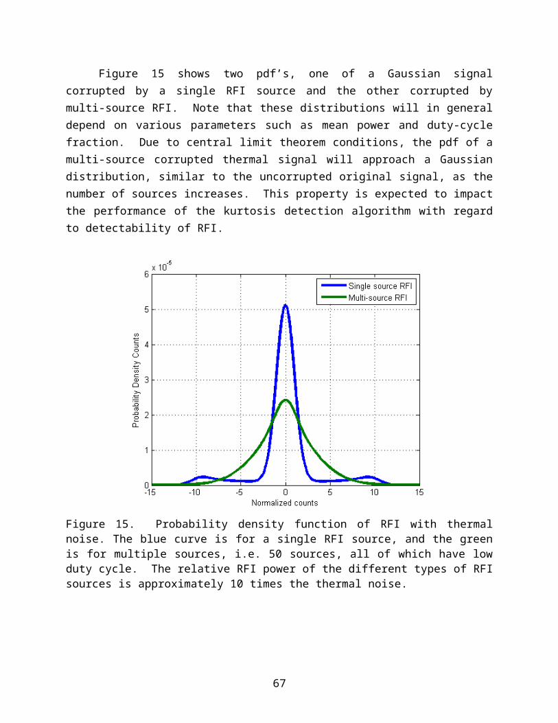
5.14 Atmospheric CorrectionThe Earth’s atmosphere affects the propagation of electromagnetic radiation via absorption, emission, and scattering. At L-band, scattering is negligible except when extraordinarily intense (hurricane intensity) precipitation is present (Ulaby et al, 1986 [TBC]), and in that case SMAP would not be attempting soil moisture retrieval anyway. We therefore consider only absorption and emission.

Three parameters (upwelling brightness Tup, downwelling brightness Tdown, and total atmospheric loss factor L) are needed to describe the atmosphere’s effect on a signal which is emitted from the Earth’s surface and received by a spaceborne radiometer. The general form of the apparent brightness temperature at the top of the atmosphere (TOA) is given by

T ap ,TOA=T up+[ (1−ε ) T down+T B ] L−1

(5.81)

where ε is the emissivity of the Earth’s surface and TB is the brightness temperature of the Earth’s surface. This equation simply says that the radiometer sees the sum of the surface

brightness TB attenuated by L, added to upwelling atmospheric brightness Tup plus the downwelling atmospheric brightness Tdown reflected off the surface and attenuated by L. At L-band at

40 degrees EIA, downwelling brightness is the same as upwelling brightness to within about 2 mK, so Tup = Tdown for our purposes. With this simplification, we can invert Equation

T ap ,TOA=T up+[ (1−ε ) T down+T B ] L−1

to obtain:

T B=T surf

T surf −T up∙ [ L ∙T ap ,TOA−(1+L ) ∙T up ]

(5.82)

where Tsurf really refers to the temperature at the bottom of the atmosphere near the Earth’s surface. Tap,TOA is the uncorrected brightness observed at TOA, and TB is the desired Earth surface brightness corrected for atmospheric effects. So only upwelling brightness, Tup, and total attenuation, L, need to be calculated.

These two parameters can also be estimated by using a global simplified atmospheric radiative transfer model. This model was developed specifically for the atmospheric correction in the SMAP L1B_TB algorithm when we discovered that the simplified Liebe model in the original Aquarius simulator was too computation intensive for SMAP purposes.

In the simplified model, upwelling brightness T up and total attenuationL, both for EIA 40°, are modeled as polynomial functions of near surface atmospheric pressure P in millibars, temperature Tsurf in degrees Celsius, and water vapor density V in grams per cubic meter:

T up=2.3058−3.2735 ×10−3T surf +4.2330 ×10−3(P−900)+1.4472 ×10−3 V(5.83)

68

L=1.0094−2.9626 ×10−5T surf +1.6521× 10−5(P−900)+1.0712 ×10−5V(5.84)

(Here, Tsurf really refers to the temperature at the bottom of the atmosphere near the Earth’s surface as opposed to the temperature of the Earth’s surface.)

These expressions were developed by matching against conventional atmospheric radiative transfer from Ulaby et al, (1981) applied to the Integrated Global Radiosonde Archive dataset from the NOAA/National Climatic Data Center (~1000000 global soundings from 662 stations including all 7 continents after filtering to those soundings that go up to at least 30km altitude). At EIA = 40°, the difference between the simplified model vs. conventional radiative transfer for Tup, and Tdown is zero mean with a 1σ standard deviation of 0.028 K and for the total atmospheric loss factor L, it is zero mean with a 1σ standard deviation of 2.110-4.

The source of the ancillary data P, Tsurf, and V will be a near real-time global weather analysis product such as the NCEP Daily Global Analyses, (surface level). A selection will be made prior to SMAP CDR based on considerations such as latency, data availability, accuracy, spatial resolution, etc.

5.15 Full transformation from antenna temperature TA to brightness temperature TB

Combining the preceding APC, Faraday, and atmospheric corrections, Equation (5.85) shows the full transformation from antenna temperature seen at the SMAP main reflector to the desired main beam brightness temperature.

[T B, v

T B, h

T B,3

T B, 4]= T surf

T surf −Tup∙ [ L∙ T ap ,TOA−(1+L ) ∙T up ]= T surf

T surf −T up∙[L∙ [(T ¿¿ ap , v+T ap ,h+Qap)/2 ¿(T ¿¿ap , v+Tap , h−Qap)/2¿0

T ap ,4 ]−(1+L ) ∙T up](5.85)

where

~~T A , p=T A , p−(1−ηp¿T Br

ηpp=v , h , 3,4¿~T A , p=

~~T A , p−Erefl , p ∙T phys ,refl

(1−Erefl , p )p=v , h , 3,4¿ [T ap , v

T ap , h

T ap ,3

T ap ,4]= A−1 ∙[

~T A , v~T A , h~T A , 3~T A , 4

] .¿(5.86)

69

6 Orbital SimulatorTo assist with radiometer L1B algorithm development, an orbital simulator capable of simulating the SMAP observing geometry, and the effects of the unwanted sources and propagation effects depicted in Figure 20, is a major risk-reduction asset. The radiometer team at Goddard obtained a copy of the Aquarius TB simulator [Le Vine, et. al, 2011] from the Aquarius Deputy PI Dr. David Le Vine, and proceeded to modify it for SMAP purposes. Although this simulator addresses all the sources and effects depicted in Figure 20, there are important differences between Aquarius and SMAP. This section provides a summary of the modifications necessary for deploying the Aquarius simulator as a SMAP simulator.

6.1 Number of antenna beamsAquarius’ 3 beams were replaced with a single beam for SMAP.

6.2 Conical scanSMAP employs a conical scan at 40 degrees EIA vs. Aquarius’ fixed beams.

6.3 Antenna patternSMAP’s 6 m antenna has a considerably narrower beam than Aquarius’ 2 m antenna. The actual pattern from the SMAP antenna design is used instead of the Aquarius patterns. To balance the spatial resolution over a footprint and simulation speed, hybrid-resolution antenna pattern is used in the orbit simulator. Within the first null-to-null beamwidth which is defined as 2.5 times 3-dB beamwidth in the simulator, the resolution of the antenna pattern is 0.1°, while beyond the region, it is 0.5°.

6.4 Land focusWhereas Aquarius’ focus is naturally the ocean, SMAP’s focus is land areas (plus selected ocean and ice sheet targets for calibration). The land TB model in the Aquarius simulator is replaced by using the microwave emission model [Njoku, et. al, 1999] which is significantly more realistic detailed regarding land cover types, and other factors to yield more realistic land TB at a spatial resolution sufficient to use the simulator to analyze effects requiring sub-pixel resolution such as geolocation.

6.5 Atmosphere modelThe Aquarius simulator employed an atmosphere model that was simplified for L-band. It was found that adding the conical scan also multiplied the number of iterations needed for the atmosphere routine. In fact, the atmosphere routine could dominate the computation time. A

70

much-simplified atmosphere model was developed and validated against almost 106 soundings in the NCDC radiosondes database [Peng, Kim, and Piepmeier, in press]. This simplified model requires only surface temperature, pressure, and water vapor as input parameters, and results in a considerable increase in computation speed.

6.6 Ancillary dataAs a result of the upgrades to the land and atmosphere modules, the input and ancillary data needs for the SMAP simulator are different vs. the Aquarius simulator. The ancillary data requirements are listed in Table 8.

Table 8. Ancillary Datasets for SMAP Orbit Simulator

Name SpatialResolution

TemporalResolution

Note

SSS 0.1° x 0.1° 6 hoursSST 0.1° x 0.1° 6 hoursWS 0.1° x 0.1° 6 hoursMask 0.1° x 0.1° 6 hours Water, land,

ice.Vegetation Water Content (VWC)

0.1° x 0.1° 1 day

IGBP Land Cover Map

0.01° x 0.01° static

Land Roughness Map 0.1° x 0.1° staticLand Surface Temp 0.1° x 0.1° 1 hourLand Soil Moisture 0.1° x 0.1° 1 hourSand Fraction Map 0.1° x 0.1° staticClay Fraction Map 0.1° x 0.1° staticOpen Water Fraction 0.1° x 0.1° staticNear Surface Air Temp

2.5° x 2.5° 6 hours

Near Surface Pressure 2.5° x 2.5° 6 hoursNear Surface Water Vapor Density

2.5° x 2.5° 6 hours

Solar Flux 1 daySun Spot Number 1 dayGalactic TB Map 0.5° x 0.5° static

7 Calibration and ValidationThe ATBDs are the primary documents for cal/val.

71

7.1 Pre-Launch Cal/Val (Antenna Temperature)The pre-L cal/val plan is detailed in The SMAP Radiometer GSFC Pre-Launch Calibration Plan, SMAP-I&T-PLAN-0013. This document is ITAR/Export controlled.

7.2 Post-Launch Cal/Val (Brightness Temperature)A separate document detailing the post-launch cal/val plans is under preparation. Here, only the basis of the major steps required to generate the L1B_TB product are described.

7.2.1 Geolocation ValidationInitially after launch, geolocation will be performed “open-loop” according to the approach described in Section 5.3.

7.2.2 End-to-end TB Calibration Using External TargetsSince a full end-to-end calibration of the SMAP radiometer including the deployed reflector can only be performed on-orbit, end-to-end TB calibration shall be performed on orbit. A desirable calibration target should be beamfilling, spatially homogeneous, temporally stable, and have a TB

value that is independently knowable via measurement or calculation to a useful level of uncertainty. SMAP is considering 3 targets: Antarctica, the open ocean, and cold space.

SMOS observations show Antarctica to be spatially homogeneous over an area of 1000 km or more. Tower-based radiometer measurements at Dome-C show sub-Kelvin temporal stability and the TB (around 200 K) appear to be predictable using simple modeling. SMAP’s polar orbit will allow viewing of Antarctica during multiple orbits every day. Aquarius and SMOS plan to also use Antarctica as a calibration target.

The open ocean is also relatively spatially uniform, with a TB around ~100 K. Knowing the TB accurately will require knowledge of the sea state over (ideally) the full width of the SMAP swath (~1000 km), as well as SST and SSS. The Aquarius forward simulator will be used to help with this calculation.

Cold space views (~monthly) are part of the SMAP mission baseline. A pitch maneuver will allow a portion of or the entire conical scan to view space. For calibration purposes, L-band maps of the radio sky from radio astronomers will be used to avoid “hot spots” and to calculate the TB seen when integrating over the SMAP radiometer solid angle. Consideration of back lobe contributions from the Earth will follow the Aquarius analysis. The TB of Antarctica will be closest to the TB of SMAP’s land target areas. Antarctica and the ocean together will provide a 2-point calibration with ~100 K separation, every day, depending on ocean conditions. Cold space will add a 3rd very cold reference point, approximately monthly, for added constraining of the calibration scale.

The TB of Antarctica will be closest to the TB of SMAP’s land target areas. Antarctica and the ocean together will provide a 2-point calibration with ~100 K separation, as frequently as

72

every day, depending on ocean conditions. Cold space will add a 3 rd very cold reference point, monthly, for added constraining of the calibration scale.

End-to-end TB calibration includes the effects of mesh emission and certain reflector-related effects. It can only be performed on-orbit after the main reflector has been deployed.

7.3 Cold sky calibration

7.3.1 PurposeCold sky (or “cold space”) is one of 3 candidate external targets available to enable end-to-end Tb calibration on-orbit by providing one of the minimum two cal points necessary for a linear calibration. We take advantage of the beam-filling, stable, and uniform TB presented by looking at deep space with the SMAP radiometer. In contrast to the other 2 external target candidates, Antarctica and the ocean, the expected TB of cold sky (~2.7 K) can be computed in an absolute sense from basic physical principles. Although SMAP does not require radiometer calibration in an absolute “truth” sense, this property of cold sky calibration (CSC) is utilized for drift detection purposes as described below. SMOS and Aquarius have both used CSC for the above purposes.

Other uses of CSC include scan bias detection because cold space should be uniform vs. scan angle (i.e., it should be a “flat field”), and on-orbit characterization of nonlinearity because together with the other 2 external cal targets, 3 temperatures are measured, potentially enabling a quadratic correction. SMOS was able to use CSC to detect and correct for drift that took 7 months to diminish as well as to use CSC for flat-field purposes. The SMAP L1B_TB simulator already incorporates the data and analysis tools to analyze the optimum locations over the Earth for the cold space viewing.

7.3.2 Temporal frequencyCSC requires the antenna main beam to point away from the Earth, so SMAP must be maneuvered into an upside-down orientation. This subtracts from Earth observing time and the maneuver carries a certain amount of risk (although CSC maneuvers have been successfully performed many times by other spaceborne radiometers). Balancing these considerations against the desire to view a very well-known external target often, it was decided to plan for monthly CSC maneuvers. This in turn drove the time frame of the drift detection/removal requirement to be monthly.

7.3.3 Sequence of maneuverIn principle, the maneuver is straightforward. To minimize uncertainty due to backlobe TB

contributions from the warm Earth, the maneuver will be performed primarily over large ocean areas (Pacific basin). A pitch maneuver is executed to reach the 180-degree upside-down orientation. The upside-down attitude should be achieved just before the spillover/far sidelobes begin to view the area of the ocean selected as ‘background’ for the cold space view. Here the

73

goal is to view cold space with a uniform, benign background. Approximately 5 minutes of CSC data are collected. Then, a second pitch maneuver is executed to return to the normal Earth-viewing orientation. Key radiometer and feed temperatures will be monitored to ensure that only readings from stable periods are used. The entire CSC maneuver is expected to be completed within a half orbit.

In order to help quantify the backlobe contribution, a variation of the above maneuver will be performed occasionally. In this case, the upside-down orientation is reached while the back lobe is still over land. The feedhorn far sidelobes, spillover, and through-the-mesh contributions will be viewing the Earth. The transition from warm land to cold ocean will allow determination of the integrated contribution of these unwanted sources. In both cases, after viewing cold space for ~5 minutes, SMAP will pitch back to normal Earth-viewing orientation to resume normal science observations.

It is expected that the same commands will be used in both cases with only the orbit location being different. The orbit locations will be known in advance and the times computed for use my Mission Operations. This same simple procedure has been used on previous missions with great success.

7.4 Subband vs. Fullband cross-calibrationRFI detection and mitigation require each of the 16 subbands (times 2 polarizations) to be radiometrically calibrated with respect to each other as well as with respect to the fullband. This imvolves the same end-to-end calibration using the same 3 external targets. Since each subband is 1/16 the bandwidth of the fullband, calibrating one subband to the same NEDT level as the fullband NEDT will require 16 times as many independent looks. High rate data mode is required to downlink all the subband measurements, and downlink data volume constraints limit the time that can be spent with the radiometer in high rate mode. The high rate data requirements are in formulation.

7.5 Scan bias correctionThe flat field property of the cold sky TB (i.e., constant TB vs. scan angle) will be subtracted from the recorded Tb and persistent correlation vs. scan angle will be considered the basic scan bias to be subtracted from normal Earth observations as a function of scan angle.

7.6 Drift detection and correctionThe uncertainty of end-to-end external cal over the range of TB used by the L2 SM retrieval (the “SM TB range” approximately 180 to 300 K) is a function of the uncertainties of the assumed TB

of the external targets plus how close (in Kelvin) the external target TB is to the SM TB range. Because the uncertainty of the cold sky TB is small and the TB value is farther away (a longer

74

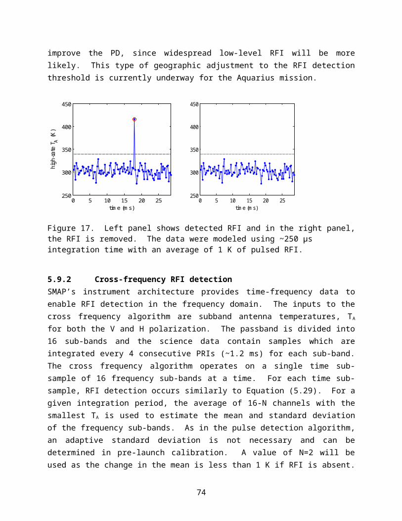
“lever arm” if you will) from the SM TB range than the other 2 external targets, a calibration using cold sky provides a calibration with smaller uncertainty than a calibration using Antarctica plus ocean. This higher accuracy monthly calibration using CSC data will be used to detect drift, defined here as the change in L1A and L1B calibration parameters after other time-dependent errors are removed. If this residual error exceeds the drift requirement of 0.4 K, adjustments will be made to the appropriate L1A and L1B calibration parameters in order to force the residual to be less than 0.4 K.

7.7 Other post-launch cal/val activities

7.7.1 General trendingAs is common for all spaceborne radiometer missions, a number of instrument and spacecraft parameters will be trended for the lifetime of the mission. This trending is particularly important during commissioning and intensive cal/val phases. The parameters will include physical temperatures of key RFE & RDE locations, the feed, noise diodes, supply voltages, spin rpm, spacecraft orbit and attitude variables, etc.

7.7.2 Comparison of measured versus expected TBA general comparison of measured versus expected TBs will be performed. Due to the large size of the radiometer footprints and the magnitude of the uncertainties for TB over land, this diagnostic will mainly be a sanity check rather than a high-accuracy tool for uncovering performance issues post-launch.

7.7.3 Intercomparison versus other radiometersIf other L-band radiometers are in orbit at the same time as SMAP, inter-comparisons will be conducted to provide additional independent information related to SMAP calibration and stability.

8 Practical Considerations

8.1.1 Variance and Uncertainty EstimatesThe radiometer error budget is documented elsewhere, (see SMAP Radiometer Error Budget Document, JPL D-61632) but a top level breakdown is given here. A number of its components vary with month and/or grid cell, so their RMS value depends on the size of the temporal and/or spatial domain (to be specified). The uncertainties described below are for the L1C_TB product and need to be translated to the L1B_TB product.

Table 9. Uncertainty in L1C_TB for 30 km x 30 km grid cells

75

Item “Allocation” now used (K) Varies withTOTAL ERROR 1.0 to 1.5NEDT 0.6 to 0.7 Grid cell’s RFI and TB

Antenna Pattern Correction 0.3Internal Calibration 0.1Polarization Rotation 0.3RFI 0.3Residual Bias 0.0 to 1.0 Month (eclipse), latitude

The APC term is derived under particular assumptions about the APC algorithm and the quality of the ancillary data which are used. These assumptions are:

(1) Earth sidelobe scene TB shall be determined to within 6 K RMS. Options to achieve this need to be studied. Includes uncertainty due to uncertain Faraday rotation of sidelobe contributions.a. Seasonal climatological model of sidelobe scene may suffice.b. If necessary, SMAP measurements of the sidelobe scene from the current, recent

past, and near future passes can be used to determine the scene TB with an uncertainty of 1.3 K (plus some uncertainty for time difference [precipitation may fall during one pass but not another] and for azimuth and incidence angle differences).

(2) Space scene TB shall be determined to within 1 K RMS. For data sources which can provide this, see: a. The source Aquarius is using (Frank Wentz or David Le Vine)b. the 2008 article “A fully sampled λ21 cm linear polarization survey of the southern

sky” and/or c. the 1999 article “A 1.4 GHz radio continuum and polarization survey at medium

Galactic latitudes.”

(3) Algorithm shall correct for the solar contribution using the nominal antenna pattern.

(4) Algorithm shall ingest pointing knowledge (whose accuracy is specified by L2-MSR-357 and L2-MSR-261) in order to reduce error in location of the sun and the earth horizon in the antenna pattern to the accuracy specified by L2-MSR-357 and L2-MSR-261.

(5) Algorithm shall flag the worst TBD% of pixels affected by solar contributions as Data Loss (so that they do not count against error budget).

(6) Algorithm shall use PRT or thermistor data to adjust nominal gain of lossier front-end components (OMT, not feed).

76

(7) Algorithm shall use modeled mesh temperature (whose accuracy is 20 C 1-sigma over time) to estimate and subtract off mesh emissions. This coarse temperature estimate meets requirements.

(8) Algorithm shall correct for antenna, OMT, and radiometer cross-pol using an estimate of the cross-pol scene temperature that is accurate to within 2 K RMS.

a. This can be accomplished using a rougher, initial estimate of the cross-pol scene temperature.

(9) Algorithm shall estimate scene TB over no more than 4 PRIs at a time so that bias due to thermal skew is negligible.

8.1.2 Test PlanSMAP is modifying the Aquarius forward simulator for SMAP purposes. It will be able to generate TB of land and ocean, including the effects of Faraday rotation, the atmosphere and, direct and reflected contributions from solar, lunar, galactic, and cosmic background sources. This TB field can be used to test the L1B_TB algorithm, although since the simulator is also slated to be used to correct for these sources, it would not be a completely-independent test of functionality and accuracy. However, many tests of the functionality and sensitivity of nearly all aspects of the L1B_TB algorithm may be checked. For example, by specifying Antarctic and ocean TB, the functionality and sensitivity of the TB calibration portion of the algorithm may be checked. Geolocation noise can be added to test the geolocation portion of the algorithm. Error handling and data range checking can all be tested prior to launch. Even simulated RFI can be added for testing purposes. SMOS and Aquarius L-band observations may also be useful, although differences in footprints, viewing geometry, etc. will limit the fidelity of such exercises.

Pre-launch testing of the RFI detection and mitigation algorithm can be broken down into three stages: 1) mitigation capability at the subsystem level; 2) detection capability at the integrated system level; and 3) end-to-end detection and mitigation performance.

Stage 1. Subsystem level (pre-integration) testing of mitigation.The out of band (OOB) rejection capabilities of the hardware must be verified in both the time and frequency domains. In the time domain, the impulse response time of the system must be sufficiently fast so that it has recovered from RFI spikes before subsequent sampling intervals. In the frequency domain, the rejection by subband filters of RFI in neighboring bands must be sufficient to isolate RFI in individual (or possibly adjacent) subband filters.

Stage 2. Integrated testing of detection.The NET and NEk (for kurtosis) performance of the fully integrated radiometer must be verified. These noise statistics will determine the false alarm rate of the detection algorithm.

77

Stage 3. End-to-End verification of detection and mitigation.Simulated controlled RFI plus gaussian noise signals should be injected in to the antenna input port of the fully integrated radiometer and the sensors ability to detect and mitigate its presence should be verified and characterized.

78

9 References

Corbella, I., F. Torres, A. Camps, N. Duffo, M. Vall-llossera, K. Rautiainen, M. Martin-Neira, A. Colliander, “Analysis of correlation and total power radiometer front-ends using noise waves,” IEEE Trans. Geosci. Remote Sens., vol. 43, no. 11, pp 2452-2459, Nov. 2005.

De Roo, R., S. Misra and C. S. Ruf, “Sensitivity of the Kurtosis Statistic as a Detector of Pulsed Sinusoidal RFI,” IEEE Trans. Geosci. Remote Sens., vol. 45, no. 7, pp 1938-1946, July 2007.

Güner, B., N, Niamsuwan and J. T. Johnson, “Performance study of a cross-frequency detection algorithm for pulsed sinusoidal RFI in microwave radiometry,” IEEE Trans. Geosci. Remote Sens., vol. 48, no. 7, pp 2899-2908, July 2010.

Ellingson, S. W., and J. T. Johnson, Airborne RFI measurements over the mid-Atlantic coast using LISA, technical report, ElectroSci. Lab., Ohio State Univ., Columbus, Jan. 2003.

Entekhabi, D. E., Njoku, P. Houser, M. Spencer, T. Doiron, J. Smith, R. Girard, S. Belair, W. Crow, T. Jackson, Y. Kerr, J. Kimball, R. Koster, K. McDonald, P. O'Neill, T. Pultz, S. Running, J. C. Shi, E. Wood, and J. van Zyl, “The Hydrosphere State (HYDROS) mission concept: An Earth system pathfinder for global mapping of soil moisture and land freeze/thaw,” IEEE Trans. Geosci. Remote Sens., vol. 42, no. 10, pp. 2184-2195, 2004.

Entekhabi, D., E. Njoku, P. O’Neill, K. Kellogg, W. Crow, W. Edelstein, J. Entin, S. Goodman, T. Jackson, J. Johnson, J. Kimball, J. Piepmeier, R. Koster, K. McDonald, M. Moghaddam, S. Moran, R. Reichle, J. C. Shi, M. Spencer, S. Thurman, L. Tsang, J. Van Zyl, “The Soil Moisture Active and Passive (SMAP) Mission”, Proceedings of the IEEE, 98(5), 2010.

Johnson, J.T., and L. C. Potter, “Performance study of algorithms for detecting pulsed sinusoidal interference in microwave radiometry,” IEEE Trans. Geosci. Remote Sens., vol. 47, no. 2, pp 628-636, Feb. 2009.

Kenney, J. F. and E.S. Keeping, "Kurtosis," Mathematics of Statistics, 3rd ed. Princeton, NJ: Van Nostrand, 1962, ch.1, Sec. 7.12, pp. 102-103.

Le Vine, D.M. Dinnat, E.P. Abraham, S. de Matthaeis, P. Wentz, F.J. “The Aquarius Simulator and Cold-Sky Calibration”, IEEE Transaction on Geoscience and Remote Sensing, 49(9), doi:10.1109/TGRS.2011.2161481, 2011

Meissner, T. and F.Wentz, “GMI calibration algorithm and analysis theoretical basis document” version F, Remote Sensing Systems, Aug 29, 2011.

79

Misra, S., P. N. Mohammed, B. Güner, C. S. Ruf, J. R. Piepmeier, J. T. Johnson, “Microwave Radiometer Radio-Frequency Interference Detection Algorithms: A Comparative Study,” IEEE Trans. Geosci. Remote Sens., vol. 47, no. 11, pp 3742-3754, November 2009.

Misra, S., R. De Roo and C. S. Ruf, “An Improved Radio Frequency Interference Model: Reevaluation of the Kurtosis Detection Algorithm Performance under Central-Limit Conditions,” IEEE Trans. Geosci. Remote Sens., in press, 2012.

National Research Council, “Earth Science and Applications from Space: National Imperatives for the Next Decade and Beyond,” pp. 400, 2007.

Njoku, E.G., Li Li, “Retrieval of land surface parameters using passive microwave measurements at 6-18 GHz”, IEEE Transaction on Geoscience and Remote Sensing, 37(1), doi:10.1109/36.739125, 1999

Niamsuwan, N., J. T. Johnson, S. W. Ellingson, “Examination of a simple pulse-blanking technique for radio frequency interference mitigation,” Radio Science, vol. 40, June 2005.

Pardé, M., M. Zribi, P. Fanise, and M. Dechambre, “Analysis of RFI issue using the CAROLS L-band experiment,” IEEE Trans. Geosci. Remote Sens., vol. 49, no. 3, pp 1063-1070, March 2011.

Park, J., J. T. Johnson, N. Niamsuwan, J. R. Piepmeier, P. N. Mohammed, C. S. Ruf, S. Misra, S. H. Yueh, and S. J. Dinardo, “Airborne L-Band Radio Frequency Inteference Observations From the SMAPVEX08 Campaign and Associated Flights,” IEEE Trans. Geosci. Remote Sens., vol. 49, no. 9, 3359-3370, September 2011.

Peng, J., Piepmeier, J.R., Kim, E.J., “Global Simplified Atmospheric Radiative Transfer Model at L-band,” IEEE Geoscience and Remote Sensing Letter, in press.

Piepmeier, J., F. Pellerano, A. Freedman, “Mitigation of terrestrial radar interference in L-band spaceborne microwave radiometers,” Proc. 2006 IEEE International Geoscience and Remote Sensing Symposium, Denver, CO, 31 Jul - 4 Aug 2006.

Piepmeier, J.R., E. J. Kim, “Calibration of passive microwave hybrid coupler-based polarimeters,” Proc. 2003 IEEE International Geoscience and Remote Sensing Symposium, Toulouse, France, vol. 2, pp 1244-1246, 21-25 July 2003.

Piepmeier, J.R., Long, D.G., Njoku, E.G., “Stokes Antenna Temperatures,” IEEE Trans. Geosci. Remote Sens., vol. 46, no. 2, February 2008.

80

Ruf, C.S., S. M. Gross and S. Misra, “RFI Detection and Mitigation for Microwave Radiometry with an Agile Digital Detector,” IEEE Trans. Geosci. Remote Sens., vol. 44, no. 3, 694-706, March 2006.

Skou, N., J. E. Balling, S. S. Sobjarg, S. S. Kristensen, “Surveys and analysis of RFI in the SMOS context,” Proc. 2010 IEEE International Geoscience and Remote Sensing Symposium, Honolulu, HI, 25 Jul - 30 July 2010.

Ulaby, F. T., R. K. Moore, and A. K. Fung, Microwave remote sensing: active and passive. Volume 1, Microwave Remote Sensing Fundamentals and Radiometry. Reading, Mass.: Addison-Wesley Pub. Co., Advanced Book Program/World Science Division, 1981.

Yueh, S. H., “Estimates of Faraday rotation with passive microwave polarimetry for microwave remote sensing of Earth surfaces,” IEEE Trans.Geosci. Remote Sensing, vol. 38, pp. 2434–2438, Sept. 2000.

81