NASA Contractor Report 3407

NASA CR 3407 c.1

Small-Angle Approximation to the’, ’ Transfer of Narrow Laser Beams in Anisotropic Scattering Media

Michael A. Box and Adarsh Deepak

CONTRACT NASs-3 3 13 5 APRIL 198 1

https://ntrs.nasa.gov/search.jsp?R=19810013375 2018-07-01T23:15:41+00:00Z

TECH LIBRARY KAFB. NM

NASA Contractor Report 3407

Small-Angle Approximation to the Transfer of Narrow Laser Beams in Anisotropic Scattering Media

Michael A. Box and Adarsh Deepak Institute for Atmospheric Optics and Remote Sensing Hampton, Virginia

Prepared for Marshall Space Flight Center under Contract NASS-3 3 13 5

National Aeronautics and Space Administration

Scientific and Technical Information Branch

1981

- _ . ..-

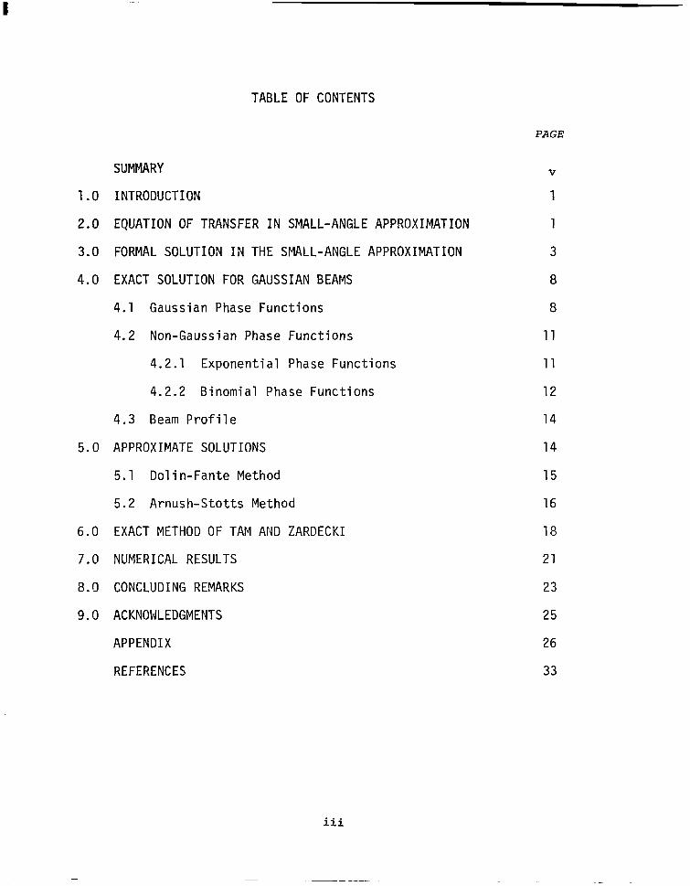
TABLE OF CONTENTS

PAGE

SUMMARY

1.0 INTRODUCTION

2.0 EQUATION OF TRANSFER IN SMALL-ANGLE APPROXIMATION

3.0 FORMAL SOLUTION IN THE SMALL-ANGLE APPROXIMATION

4.0 EXACT SOLUTION FOR GAUSSIAN BEAMS

4.1 Gaussian Phase Functions

4.2 Non-Gaussian Phase Functions

4.2.1 Exponential Phase Functions

4.2.2 Binomial Phase Functions

4.3 Beam Profile

5.0 APPROXIMATE SOLUTIONS

5.1 Dolin-Fante Method

5.2 Arnush-Stotts Method

6.0 EXACT METHOD OF TAM AND ZARDECKI

7.0 NUMERICAL RESULTS

8.0 CONCLUDING REMARKS

9.0 ACKNOWLEDGMENTS

APPENDIX

REFERENCES

V

1

1

3

8

8

11

11

12

14

14

15

16

18

21

23

25

26

33

iii

LIST OF ILLUSTRATIONS

Figure

1

2

3

4

5

6

7

Title

Normalized phase function p vs. a$ for four model phase functions . . . . . . . . . . . . .

no& vs. y for four model phase functions and for the Arnush-Stotts approximation . . . .

Amplification factor A vs. geometry factor G for the Gaussian phase function. . . . . . . . .

Normalized power received vs. scattering optical thickness for the Gaussian phase function. . . .

Amplification factor A vs. geometry factor G for two values of TS and three model phase functions

Page

. . . 34

. . . 35

. . . 36

. . . . 37

for our approach and the Arnush-Stotts approximation . . 38

Subtracted amplification factor (A - 1.0) vs. geometry factor (G) for T = 1.0 . . . . . . . . . . . . 39

Subtracted amplification factor (A - 1.0) vs. geometry factor (G) for -c = 5.0. . . . . . . . . . . . . 40

iv

SUMMARY

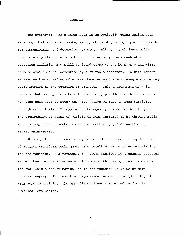
The propagation of a laser beam in an optically dense medium such

as a fog, dust storm, or smoke, is a problem of growing importance, both

for communication and detection purposes. Although such ilense media

lead to a significant attenuation of the primary beam, much of the

scattered radiation may still be found close to the beam axis and will,

thus,be available for detection by a suitable detector. In this report

we examine the spreading of a laser beam using the small-angle scattering

approximation to the equation of transfer. This approximation, which

assumes that most photons travel essentially parallel to the beam axis,

has also been used to study the propagation of fast charged particles

through metal foils. It appears to be equally suited to the study of

the propagation of beams of visible or near infrared light through media

such as fog, dust or smoke, where the scattering phase function is

highly anisotropic.

This equation of transfer may be solved in closed form by the use

of Fourier transform techniques. The resulting expressions are simplest

for the radiance, or alternately the power received by a coaxial detector,

rather than for the irradiance. In view of the assumptions involved in

the small-angle approximation, it is the radiance which is of more

interest anyway. The resulting expression involves a single integral

from zero to infinity; the appendix outlines the procedure for its

numerical evaluation.

V

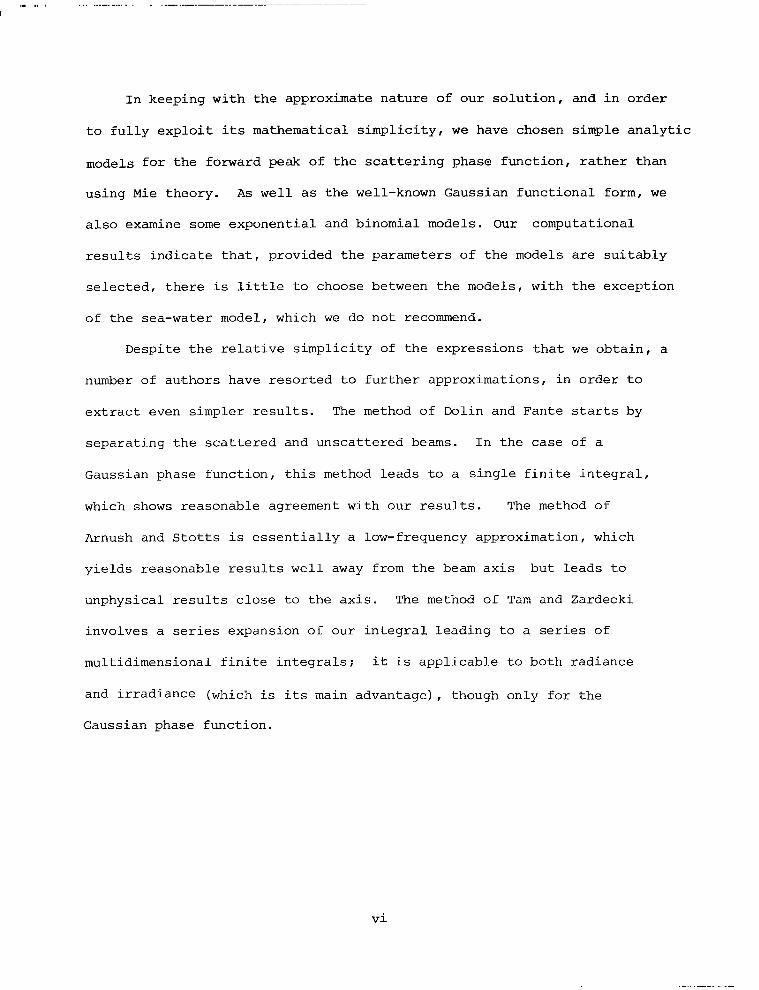
In keeping with the approximate nature of our solution, and in order

to fully exploit its mathematical simplicity, we have chosen simple analytic

models for the forward peak of the scattering phase function, rather than

using Mie theory. As well as the well-known Gaussian functional form, we

also examine some exponential and binomial models. Our computational

results indicate that, provided the parameters of the models are suitably

selected, there is little to choose between the models, with the exception

of the sea-water model, which we do not recommend.

Despite the relative simplicity of the expressions that we obtain, a

number of authors have resorted to further approximations, in order to

extract even simpler results. The method of Dolin and Fante starts by

separating the scattered and unscattered beams. In the case of a

Gaussian phase function, this method leads to a single finite integral,

which shows reasonable agreement with our results. The method of

Arnush and Stotts is essentially a low-frequency approximation, which

yields reasonable results well away from the beam axis but leads to

unphysical results close to the axis. The method of Tam and Zardecki

involves a series expansion of our integral leading to a series of

multidimensional finite integrals; it is applicable to both radiance

and irradiance (which is its main advantage), though only for the

Gaussian phase function.

vi

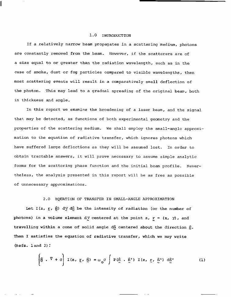
1-U INTRODUCTION

If a relatively narrow beam propagates in a scattering medium, photons

are constantly removed from the beam. However, if the scatterers are of

a size equal to or greater than the radiation wavelength, such as in the

case of smoke, dust or fog particles compared to visible wavelengths, then

most scattering events will result in a comparatively small deflection of

the photon. This may lead to a gradual spreading of the original beam, both

in thickness and angle.

In this report we examine the broadening of a laser beam, and the signal

that may be detected, as functions of both experimental geometry and the

properties of the scattering medium. We shall employ the small-angle approxi-

mation to the equation of radiative transfer, which ignores photons which

have suffered large deflections as they will be assumed lost. In order to

obtain tractable answers, it will prove necessary to assume simple analytic

forms for the scattering phase function and the initial beam profile. Never-

theless, the analysis presented in this report will be as free as possible

of unnecessary approximations.

2.0 EQUATION OF TRANSFER IN SMALL-ANGLE APPROXIMATION

Let I(z, E, 2) dy % be the intensity of radiation (or the number of

photons) in a volume element d,V centered at the point z, r = (x, y), and w

travelling within a cone of solid angle d$ centered about the direction 3.

Then I satisfies the equation of radiative transfer, which we may write

(Refs. land 2):

[fi . v + cJ] I(z, E, $) =woo 1 P'$ . $') I(z, 5, $') d$' (1)

2

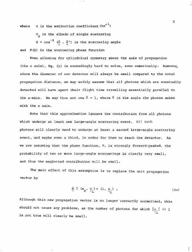
where -1

(5 is the extinction coefficient (km 1

w o is the albedo of single scattering

$ = cos-l '5 . 2' n ) is the scattering angle

and P(a) is the scattering phase function

Even allowing for cylindrical symmetry about the axis of propagation

(the z axis), Eq. (1) is exceedingly hard to solve, even numerically. However,

since the diameter of our detector will always be small compared to the total

propagation distance, we may safely assume that all photons which are eventually

detected will have spent their flight time travelling essentially parallel to

the z-axis. We may thus set cos 8 = 1, where 8 is the angle the photon makes

with the z axis.

Note that this approximation ignores the contribution from all photons

which undergo at least one large-angle scattering event. All such

photons will clearly need to undergo at least a second large-angle scattering

event, and maybe even a third, in order for them to reach the detector. As

we are assuming that the phase function, P, is strongly forward-peaked, the

probability of two or more large-angle scatterings is clearly very small,

and thus the neglected contribution will be small.

The main effect of this assumption is to replace the unit propagation

vector by

ii E (n n I+ z' -J- (1, n 1 -1

. (2a)

Although this new propagation vector is no longer correctly normalized, this

should not cause any problems, as the number of photons for which 1~~1 << 1

is not true will clearly be small.

3

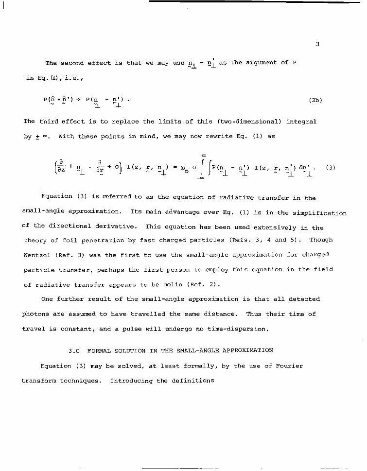
The second effect is that we may use c1 - $- as the argument of P

in Eq. (l), i.e.,

(2b) P($ l fi') + P(n - n') . ..a - "I "-L

The third effect is to replace the limits of this (two-dimensional) integral

by + 00. With these points in mind, we may now rewrite Eq. (1) as

a -+n aZ a+0

-1 * ar I(z, r,n)=w 0 P(n - n') I(z, r, n') dn' . (3) . --I O ff --I --L - -1 -1 -co

Equation (3) is referred to as the equation of radiative transfer in the

small-angle approximation. Its main advantage over Eq. (1) is in the simplification

of the directional derivative. This equation has been used extensively in the

theory of foil penetration by fast charged particles (Refs. 3, 4 and 5). Though

Wentzel (Ref. 3) was the first to use the small-angle approximation for charged

particle transfer, perhaps the first person to employ this equation in the field

of radiative transfer appears to be Dolin (Ref. 2) -

One further result of the small-angle approximation is that all detected

photons are assumed to have travelled the same distance. Thus their time of

travel is constant, and a pulse will undergo no time-dispersion.

3.0 FORMAL SOLUTION IN THE SMALL-ANGLE APPROXIMATION

Equation (3) may be solved, at least formally, by the use of Fourier

transform techniques. Introducing the definitions

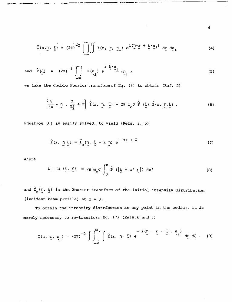
co

hbn, 5, = (2T)-2 J JJi

I(z, r, n1) e j-07-r + E.-n11 dr dn _ _ - _ .., s _ . ..I -Co

and G(c) = (HIT)-' i c-n,

P(zL) e ""Idn , --L

-Ccl

we take the double Fouriertransformof Eq. (3) to obtain (Ref. 2)

Equation (6) is easily solved, to yield (Refs. 2, 5)

z(Z, rl,E) = ;o(!, 5 + z 2) e -oz+n

w -

where

and Tot]?, 5) is the Fourier transform of the initial intensity distribution

(incident beam profile) at z = 0.

TO obtain the intensity distribution at any point in the medium, it iS

merely necessary to re-transform Eq. (7) (Refs.6 and 7)

4

(4)

(5)

(6)

(7)

(8)

00

-2 JJJJ -i(n.r+E.n)

I(z, r, n ) = (2lT) - -I

^I(z, rl, C;) e w w - -l dn dc . (9) w - w u -co

5

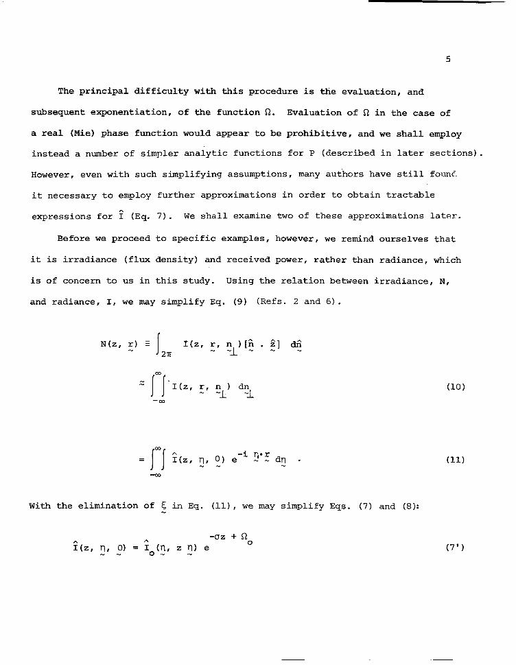
The principal difficulty with this procedure is the evaluation, and

subsequent exponentiation, of the function G?. Evaluation of fi in the case of

a real (Mie) phase function would appear to be prohibitive, and we shall employ

instead a number of simpler analytic functions for P (described in later sections).

However, even with such simplifying assumptions, many authors have still fount

it necessary to employ further approximations in order to obtain tractable

expressions for 1 (Eq. 7). We shall examine two of these approximations later.

Before we proceed to specific examples, however, we remind ourselves that

it is irradiance (flux density) and received power, rather than radiance, which

is of concern to us in this study. Using the relation between irradiance, N,

and radiance, I, we may simplify Eq. (9) (Refs. 2 and 6).

N(z, r) E J I(z, r, n )[^n . 2^] aii 21T

--.- - -

co ,” J I. I(z, r, n ) dn - -I -I

-co

Co JJ A = I(z, q, 0) ewi 'I': dn - w . -00

With the elimination of 5 in Eq. (ll), we may simplify Eqs. (7) and (8):

-uz + R %z, n, 0) = ;o(9, 2 nl e

0 . -

(10)

(11)

(7')

where n 0

6

(8’)

Equation (11) can now be further simplified by an appeal to symmetry. Since

P($) clearly depends only on the scalar In ], and not on the vector n , G will "I "I

similarly be a scalar function, as will fi . Similarly, if we assume that the 0

incident beam profile is circularly symmetric, then fo(!, z n) will also be

a scalar function of T). Thus ?(z, T-I, 0) will be a scalar function, and Eq. (11)

becomes

J 00

N(z, r) = 27r 0

Jo(n r) ?(z, n, 0) rl drl a

From Eq. (11') we see immediately that N is a scalar function of r, as we

would expect from the above symmetry arguments. A more tractable expression

for the case of a d-function beam will be given in Eq. (31).

In most instances, of course, what we are most interested in (and what

we physically measure) is the power received by some detector. This will

involve the integration of Eq. (11') over the area of the detector, perhaps

modulated by a response function. If we assume a coaxial, circular detector

of radius R, with a flat response, then we have

R Hz I R) = 2Tr J N(z, r) r dr

0

J 03 = 4rr2 eDuz R

Jl(n R) To('l, s 1) e OR dn .

0

(11’)

(12)

7

This result should prove amenable to numerical integration, especially if

a relatively simple expression for R. can be obtained. Sample results will

be presented 'below.

One useful result which can be obtained analytically, is the total power

crossing a surface z = constant:

co P(z, 03) = JJ N(z, r) dr - w

-CO

m -in-r = JJJJ zz, n, 0) e _ - dn dr - ..a _ ..,

--co

= 4T2 ^I(z, 0, 0)

-uz + 2Tr wou z G(O) = 4T2 To(O, 0) e

-(l = F. e

- wo) uz (13)

where F 0

is the incident total power, and we have used the fact that G(O) = (2~)~l.

From Eq. (13) we see that the only energy removed from the beam is that lost

by absorption -- i.e., there is no backscatter.

One further parameter which will often prove useful is the beam spread,

which we may define as

<r2> = N(z, r) r3 dr / N(z, r) r dr

(1 - wo) uz = HIT F-o1 e N(z, r) r3 dr . (14)

4.0 EXACT SOLUTION FOR GAUSSIAN BEAMS

At the entrance to a scattering medium, a laser beam profile can often

be adequately represented by a Gaussian functional form, both for the radial

distribution, and the angular divergence. Thus we have

Io’z, III) = F. B2 y2 IT-~ exp(-B2 2: - Y2 z2) .

This may be easily transformed, and, in particular, we have

:Oh z rj) = Fo(2~)-2 exp (-q2 / 4 y2 - z2 T12/ 4 B2) *

(15)

(161

In general, the laser beam profile will be well collimated, so that 6 and y

will be large. The inclusion of Eq. (16) in Eq. (12) will in no way complicate

the numerical integration, though in our examples later we will allow both to

go to infinity, so as to reduce the number of parameters whose influence should

be examined. In all practical calculations, however, realistic values of both

parameters should be included.

4.1 Gaussian Phase Functions

A Gaussian functional form is also often employed to describe P(Q), since

exact Mie theory is clearly somewhat impractical. Thus we choose to write

P(Q) = 2u2e 22

-a lJ / 21T . (17)

9

The ~1 is an adjustable parameter, which controls the shape of the forward peak,

-2 and is related to the rms scattering angle $ defined as

2 co

l) =2,lT J

P(W Q3 d'# a (17a) 0

It is easily shown that for the Gaussian case

Q2 = a-2 . (17%)

(Though c1 will usually be large, it will rarely, if ever, be as large as

B or y-1 Taking the Fourier transform of Eq. (17) , we find

J co kg = J (5 $J) p(q) '!' dJ, 0 O

2 2 = e -5 14 a , 2n

and hence R = -1

0 woo n a Jji-erf (zr1/2a)

where erf is the well-known error function.

Substituting Eqs. (16) and (19) into (12) we find

P(Z, R) = F. R (rl R) exp [LII,~ i7 -1

c1 fi erf (zQ/2c)

- uz - n2/4 y2 - z 2 n2/4 B2] drl .

(5')

(18)

(19)

(20)

,,_- .-_--_- ..--_._-_-

10

Equation (20) is an exact equation, which is solved numerically for various

values of I?I and y. Here, we make a simplification in Eq. (20) and consider

the limiting case of (3, y + 03. This physically implies that the beam is

collimated and has zero width in space. Then by making the variable changes

-c=uz

‘I =w T S 0

-y LQ G = R/z 0j.J )

X=rlR

Equation (20) can be reduced to

J 03 Hz, R) = F. emT J1o() -G’ ITS h q-l erf (x/2G)] dx . 0

(21)

(22)

The power of the unscattered beam at an optical depth of 'c is, of course,

-T Foe . Thus, the presence of forward scattering has increased the detected

power by the factor

J co A(T

S’ G) =

0 J,(x) exp ~~ Jn. G x I- -1

erf(X/2G) dx . I

(23)

A, which we call the amplification factor, is a function of two parameters;

T S’

the scattering optical thickness, and G, the geometry factor.

-.-- . . .-.. ._-.--..--- .-- .--..-.-.-.__.. ---.-.-_---- __..- A

11

Finally, we may obtain the beam spread by substituting from Eqs. (11) and

(16) into Eq. (14):

2 <r > = T -2 s z2/3cr2 + z2/B2 + y . (24)

In general, the first term should dominate, except perhaps close to the

point of entry into the medium.

4.2 Non-Gaussian Phase Functions

Although the Gaussian form in Eq. (17) is a popular model for the

forward peak of the phase function, it is often a good idea to examine other

models, to make sure that none of the results are simply an artifact of the

Gaussian model. In this section, therefore, we shall examine a number of

other functional forms which may be (and have also been) used to model

anisotropic phase functions. We shall follow essentially the same steps as

in the previous section, and present only the results, unless further

explanation is necessary.

4.2.1 Exponential Phase Functions

i) P(Q) = Ct2 e -a 52,

G(5) = a3(a2 + 5 ) 2 -3/z , 2n

i-z0 =T s (1 + y2/6)-1'2

where

(25a)

(2%)

(25~)

(26)

12

Thus

and

ii)

Hence

J co A(T G) =

iI 2 -l/2

S’ J (Xl exp TS (1 + X2/6 G ) 0 l 1 dx (Ed

<r2> = 2 Ts z2/a2 + z2/a2 + y -2 (25e)

P(Q) = CX 1cI-l e-" '/2* (27a)

S(C) = cl(cx2 + 52)-l/2 / 2lT (2%)

i-2 0

= kc! -ls y-l 2 1/2 In [y/fi+(l+fy) J. (27~)

J a, A(T

S’ G) = o Jl(X) exp TS

1 &Gx

1 2 -2 1/2 -1ln x/Gfi+(l+yx G )

L1 II dx (27d)

<r2> = 2 T S

z2 / 3 a2 + z2 / E2 + T2.

Note that, although Eq. (27a) implies'P(0) = co, the inclusion of the correct

solid angle factor leads to a finite result for the amount of light scattered

through any angle. In fact, Eq. (27a) has been employed by Bravo-Zhivotovskiy

et al. (Ref. 6) to model the phase function of sea water.

4.2.2 Binomial Phase Functions

This time, we consider phase functions based on the functional form

(1 + cx21J2p -l. We will need the result that

J m

J,(T-#) (1 + cL2Q2)-'-l I# d$ = (T-I/~c# KU (?-l/a) / cr21w + 1) 0

(28)

where K is the modified Bessel function of the second kind. Thus if u

.__- ----.-- ..-- --

p,($) = 2 p a2 (1 + c(2$2P-1 / 27r

52 =TS 0

,,LZ rlFc + $) [Kp (y') LF(-l(Y') + KP-l(y') LFI(g)I ' r(')

where y' = YJi=

and LU is the modified Struve function of order 1J.

The expression for A may be easily written down. For 1-I > 1, we may

obtain the beam spread:

<r2> = fs Z2/3 Cr2(l.l - -2 1) + z2/B2 + Y .

Note that if 1-1 is an odd'half-integer, Eq. (29c) may be expressed in terms

of exponential functions. For example, for p = 3/2 we find

Qo(3/2) = -cS [2 fi y -1 _ .-Y/G (1 + 2 fiy-lg

13

(29a)

(29b)

(29c)

(29d)

(30)

A(Ts, G) = J,(x) exp { Ts 2 P- 2Gx-l-e -X/Gfi

(1+2 fi Gx-l)]) dx, (30')

14

4.3 Beam Profile

The spreading of a laser beam in a forward-scattering medium can be

most simply described via the beam spread parameter, <r2> , which we have

derived above. However, the profile of the expanding beam is also of interest

and will now be considered.

The formal expression for irradiance versus distance from the axis is

given by Eq. (11'). In most cases, this expression is well-behaved. However,

in the special case of 6, y + 03, Eq. (11') will diverge. An alternative

expression for N(r) may be obtained either by an integration by parts of Eq. (11')

or by differentiating Eq. (12). Adopting the second approach and setting

1 = Fo(27r) -2

0 , we obtain

1 dP N(r) = - - 27TR dR

J co i-2 =- (2Tr)-1 F rm2 e-'

0 0

J1(x) eOfi;ydx (31)

where the prime denotes differentiation of fro with respect to y (Eq. 26). With

the exception of the sea-water phase function, R. goes as y -1

for large y, and

-2 so Q; goes as y , and convergence is assured.

5.0. APPROXIMATE SOLUTIONS

In an effort to simplify the above analysis, several authors have

employed a number of approximations. In this section we shall examine two

of these approximations, neither of which appears to be particularly useful

in our problem.

15

5.1 Dolin-Fante Method

Dolin (Ref. 8) and Fante (Ref. 9) have argued that the angular shape of

the scattered intensity should be a much more slowly varying function than

PQJ) I and have thus extracted it from the integral on the right side of Eq. (3).

After separating the scattered intensity from the unscattered, and Fourier

transforming, they arrive at the following expressions

F”(z, rl, 0) = e -uz To’!, z 0) w -

Z

2% n, 0) = :o'zv z n) - J Z

and dz' exp [- Cr z' - J A(t, rl, z n) dtl - w - - 0 zl

l wou G 117 (z - z’,l

where X(t, T-l, 2

+ (1 - wo)o

Z

X(t,u,zv)dt 2

=& won/J T-l2 (z - -

- Z’) 3 + (1 z’

- wo) (5 (z - z’)

(32a)

(32b)

(33a)

(3%)

2 and $ is defined by Eq. (17a).

Equations (32) and (33) may now be inserted in Eqs. (11) or (12) as required.

Although G is no longer exponentiated, this result is complicated by the

additional (finite) integration over z'. In the case of a Gaussian phase

function, it is possible to reverse the orders of these two integrals, and

perform that over n, to give

1 WOT

A=e -WT I

dt exp [w 'c t - G2/(t woT t3 + t2)] . O 0 0

(34)

16

Our calculations show that this approximation is reasonably accurate,

except in those situations where T is large and G is small. In section 7

(Numerical Results), we will compare the predictions of Eq (34) with those

of Eq. (23). As it is not possible to perform any of the integrals for

any of the other phase function models, we have limited our examination

of this approximation to the case of the Gaussian phase function.

5.2 Arnush-Stotts Method

In order to extract analytic answers, Arnush (Ref. 10) and Stotts

(Ref. 11, 12) have expanded G to second order before performing the integration

to obtain R. (Series expansion of R would yield the same result.) Arnush

has used Bravo-Zhivotovskiy's (Ref. 6) sea water phase function, Eq. (27a),

while Stotts originally used a Gaussian phase function, Eq. (17), and more

recently the sea water phase function. This approximation is sufficient

to provide the correct values for both P(z,m), and <r2>.

We start by re-writing the definition of R as follows 0

ilo = 2.F cd0 uz (?-)z)--l J rlz

.!?(t) dt 0

= 2Tr w. uz (qz) -1 pz

J

co

Jo 0 Jo(t$) P(q) $ d$ dt .

Expanding Jo as a power series leads to

- R. = w. uz (1 - T12z2 Q2/12 + . . .)

where 7 is defined by Eq. (17a).

(35)

(36)

17

It is complicated, but reasonably straightforward to obtain the following

expression for the beam spread parameter:

<r2> = $ u. (5 z3 J12 + z2/B2 + y2. (37)

Ignoring the h,igher order terms in Eq. (361, we may insert this expression

into Eq. (11') to obtain

N(z, r) = F. exp [- (1 - wo) T - r2/<r2>] / 7T <r2> .

Similarly, integration of Eq. (12) leads to

-(1 P(Z, R) = F. e

- uoh L- l-e

-R2/<r2> 1 . Ignoring B and y, we may re-express Eq. (39) in more familiar terms

-(1 P(z, R) = F. e

- Uo)T exp (- 3 G2 Ts) , ‘1

i.e., A0 S’

- exp (- 3 G2 TV) . 'I

(38)

(39)

(39’)

(40)

Expansion of Q. to second order in y is equivalent to an asymptotic

expansion to second order in G -1 -1 ,orR . Thus we may expect this approximation

to be accurate for large values of G or R. However, its behaviour for small

values of these parameters is quite different from that of the exact results

18

quoted in previous sections. Thus we cannot expect this approximation to

prove particularly useful for our problem, as shown later by numerical comparisons.

In fact, one finds values of A which are less than unity!

For our problem, of course, we are concerned with small values of R and G,

and hence we are interested in the behayiour of R o for large values of yI i.e.,

its asymptotic expansion. The phase function model of Eq. (27a) does not have

an asymptotic expansion, due to the fact that P(0) = 03. For the other cases

we may easily show that

s-2 0

- Ts G/Y (41)

J 03

where G = 2lT P(Q) W/a . (42) 0

Thus for a Gaussian (Eq. (17)), q = JTr; Eq. (25a) gives e = 1; and Eq. (29a)

gives q = 1~ B($,p + $), where B is the beta function. (For 1-1 = $ , for example,

ij = 2.)

For large values of y, the Arnush-Stotts approximation to fi 0 goes to

(minus) infinity, and so we cannot expect this approximation to accurately

predict the power received by a small detector.

6.0 EXACT METHOD OF TAM AND ZARDECKI

The method of Tam and Zardecki (Ref. 7) is exact, at least in principle,

but requires the evaluation of multidimensional integrals, the order of which

is equal to the order of multiple scattering involved. We will restrict this

discussion to the case of the Gaussian phase function only.

II

19

The Tam and Zardecki method consists in expanding exp (fro) in a Taylor

series, before performing the integration over z' (Eq.&q. Thus, inserting

Eq. (18) in Eq. (8'), and performing the Taylor expansion, yields

exp (Ro) = 1 + El c

Z Z m - -*-

m J J dzl .-- dzm exp { -n2 isl Z: / 4a21. (43) zm!O 0

We may now perform the inverse Fourier transform (Eq. 11') to yield

where

and

where

m

N(z, r)AF e 0

Nm(z, r)

No = z2 B2 y2

exp (- r2 2 2

z2 y2 + fi2 Byl

z2 y2 + B2

(44)

(45)

1 1 N = -*- m J J 0 0 dzl

- -* dzm A -' m exp [_r2/z2 Am-] (45b)

A -2 'I 2 = c1 iii1 i Z m +B

-2 -2 -2 +z y * (45c)

We may note in particular that N 1 may be evaluated analytically in terms

of the error function. The resulting expression is quite complicated, except

in the case where (3 and y go to infinity, in which case we get

where

N1(zr r) = a2 Jn [l - erf(g)] / 2g

g = r a/z .

(46a)

(46b)

20

Turning our attention to the power received, we obtain an expression

similar to Eqs. (44) and (45), viz.

c p(z, R) = F. e-T ? -

m=g m'! pm(z, RI

2 2 2 whereP =

0 l-expI- R 6 Y

z2 y2 + B2 1

and ', = cress 1: dzlsss dzm (1 - exp [-R2/z2 /L,]} .

(47)

(48a)

(48b)

Note that, from Eqs. (47) and (48), Eq. (13) may be obtained trivially.

As with N 1'

P1 is also analytic , and in the simple case of B, y + m, we obtain

2 p1 (z, R) = l- eS + G hT [l - erf(G)] .

The number of terms required for the convergence of the series in Eqs. (44)

and (47) grows steadily with Ts, and so in some casesfor large optical thicknesses

it may become prohibitively expensive to use it. Nevertheless, these results

have one use in that Tam and Zardecki (Ref. 13) have shown that the mth order

terms in Eqs. (44) and (47) correspond to the contribution from mth order

scattering. This in itself is a useful result.

Another use suggests itself, however. The Gaussian phase function is simply

a model, with the parameters a and W 0

available for adjustment to match "real"

II-

21

scattering patterns. Since we now have a simple expression for the singly

scattered contribution, we may compare it with that produced by a real phase

function and adjust cc and w. accordingly. Then we may use the results outlined

above to estimate the multiply scattered contribution from such a phase

function. Comparisons with second and higher order contributions ,are also

possible. This should increase our confidence in the worth of results obtained

from a model phase function.

7.0 NUMERICAL RESULTS

In this section, we shall present some typical results based on our exact

formulation and the Arnush-Stotts type approximate method from selected computa-

tional results. We shall examine 4 phase function models: Gaussian (Eq. 171,

both exponential models (Eqs. 25a and 27a), and the binomial model with u = 3/2

(Eq. 29a). To simplify discussion, we shall refer to the phase function model

of Eq. (25) as the exponential model, and that of Eq. (27) as the sea-water model.

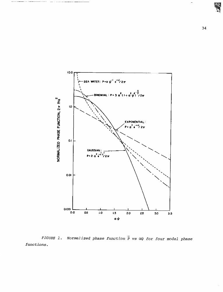
We start by examining the phase functions themselves. It is, of course,

much simpler to plot the normalized phase function, I;, rather than P, where 5

is defined by

G = 2lT P / or2. (50)

Unlike P, p is now a function of only one variable, C#. In Figure 1, we plot

P against o$, for 0 5 cw$ s 3.5.

LL

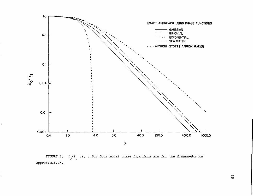
The next function we examine graphically is Qo. In Fig. 2 we plot

no/Ts against y for all 4 phase functions, as well as the Arnush-Stotts

approximation. From this log-log plot, the asymptotic behavior of the 4

phase functions is apparent, particularly that of the sea-water phase function,

which has no asymptotic expansion. Although it is not obvious from this figure,

the curve for the binomial phase function actually lies slightly above the

sea-water curve for y values less than about 3. Finally,we note that for y

values greater than 2, the results obtained by the Arnush-Stotts approximation

differ markedly from those by our exact formulation, rapidly approaching large

negative values for y greater than 4.

We now turn to a discussion of the amplification factor, A, and the

power received, P, as predicted by these 4 models, and also the Arnush-Stotts

approximation. We have evaluated both A and P for G between 0.01 and 1.0, and

~~ between 0.5 and 15.0. (Throughout, we have assumed B, y + 03.)

In the Appendix to this report, we have included a listing of the FORTRAN

program used to generate this data, along with a brief explanation and sample

output.

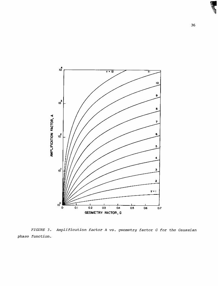
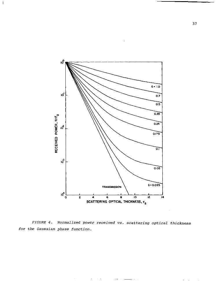
In Figure 3 we plot A against G for a series of IS values, for the

Gaussian model. In Figure 4 we plot P against Is (assuming unit incident

power) for a series of values of G, again for the Gaussian model. Also shown

on this plot is the transmission, T, which represents the power that would

be received if all scattered light was lost. These two graphs clearly

indicate the important role that forward scattering can play in the detection

of transmitted beams, especially for optical thicknesses of the order of

10 or higher.

23

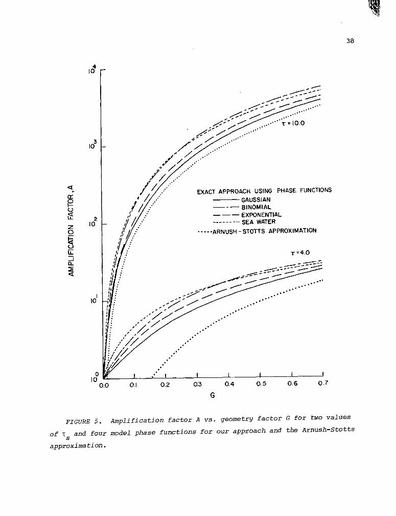
In Figure 5 we plot A as a function of G for IS = 4.0 and 10.0, for

all 4 model phase functions, for our formulation as well as the Arnush-Stotts

approximation. In the latter case, one finds values of A which are less than

unity. Note that the binomial and sea water curves cross for both I values S

(cf. Fig. 2). For large values of G, we see that there is little to choose

between the four phase function models.

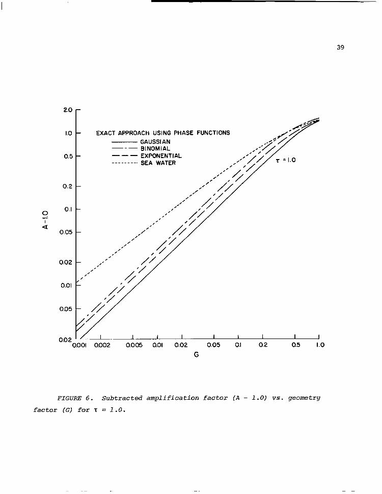
In Figure 6, we plot (A - 1.0) against G in log-log form for 'c = 1.0, in

order to emphasize the linear relationship implied by Eq. (A3) in the Appendix.

We see that for G less than 0.3, the integral term in Eq. (A3) makes a negligible

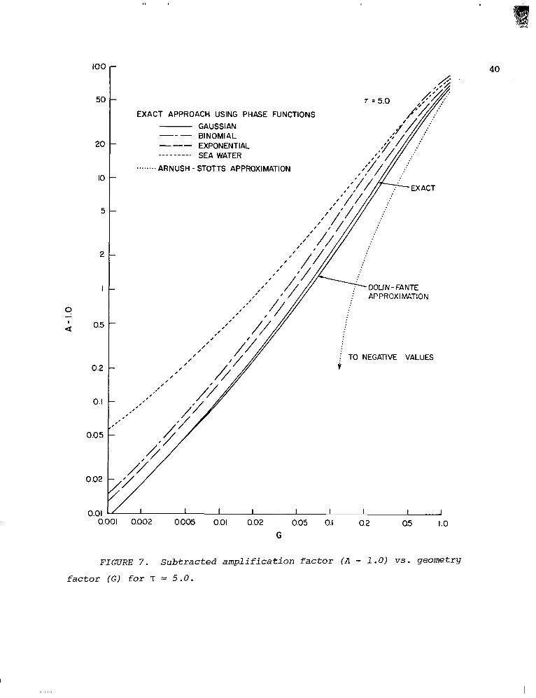
contribution. In Figure 7, we plot (A - 1.0) against G for I = 5.0. Here we

see that the integral term in Eq. (A3) is starting to make a contribution. Also

in this graph we have included the Arnush-Stotts and Dolin-Fante approximation

results. The Dolin-Fante result was not included in Figure 6 as it could not

be distinguished from the exact result for the Gaussian phase function.

8.0 CONCLUDING REMARKS

The propagation of a laser beam in an optically dense medium such

as a fog, dust storm, or smoke is a problem of growing importance, both for

communication and detection purposes. Although such dense media lead to a

significant attenuation of the primary beam, much of the scattered radiation

may still be found close to the beam axis and will, thus, be available for

detection by a suitable detector,

In this report, we have examined the spreading of a laser beam using the

small-angle scattering approximation to the equation of transfer. This

approximation appears eminently suited for the study of beam propagation in

fog, dust, or smoke media, where the scattering phase function is highly

24

anisotropic. As well as the standard Gaussian model phase function, three

other model phase functions have also been examined. The Gaussian functional

form was used to describe the initial beam spread and profile, although the

analysis is somewhat simpler (and the resulting expressions tidier) if the

limiting case is taken.

All the numerical results presented in this paper have been based on

the assumption of a narrow, collimated beam. We may remark, however, that

the results and expressions presented in this report (e.g., Eq. 20) may be

applied with full generality.

We have also examined a number of approximations which have been used to

further simplify the expressions we have derived. The Arnush-Stotts

approximation is quite suitable for use in the asymptotic regions, at large

distances from the beam axis. However, the behavior of the solutions close to

the beam axis is governed by the parameter q, the zeroth moment of the phase

function. This moment weights the contribution from scattering through very

small angles far more highly than does the parameter I$" , the rms scattering

angle, or third moment. In fact, for small R (i.e., small G), one may

expand Eq. (23) to first order (cf. Eq. A3)

A(Is,G) = 1 + -rs ; G + . . .

Finally, we may remark that the method proposed by Tam and Zardecki makes

a useful contribution by providing a connection between real (Mie) phase

functions, and the parameters which must be used in the model phase functions

used in this report. Further work on the applications of this method is

recommended.

25

ACKNOWLEDGMENTS

The valuable discussions with Drs. B. J. Anderson, NASA-Marshall Space

Flight Center, and Gerald C. Hoist, Chemical Systems Laboratory, and the

support'of this work by NASA Contract NAS8-33135, are hereby gratefully

acknowledged.

26

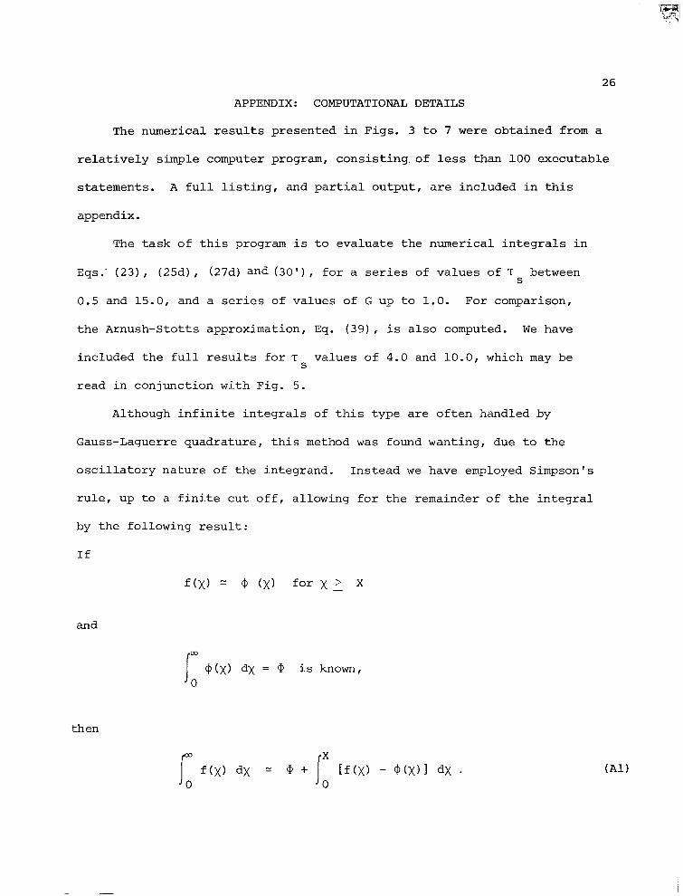
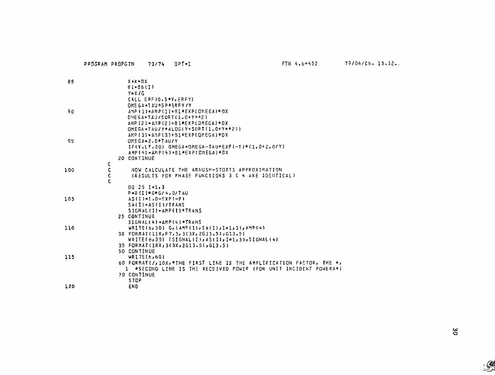
APPENDIX: COMPUTATIONAL DETAILS

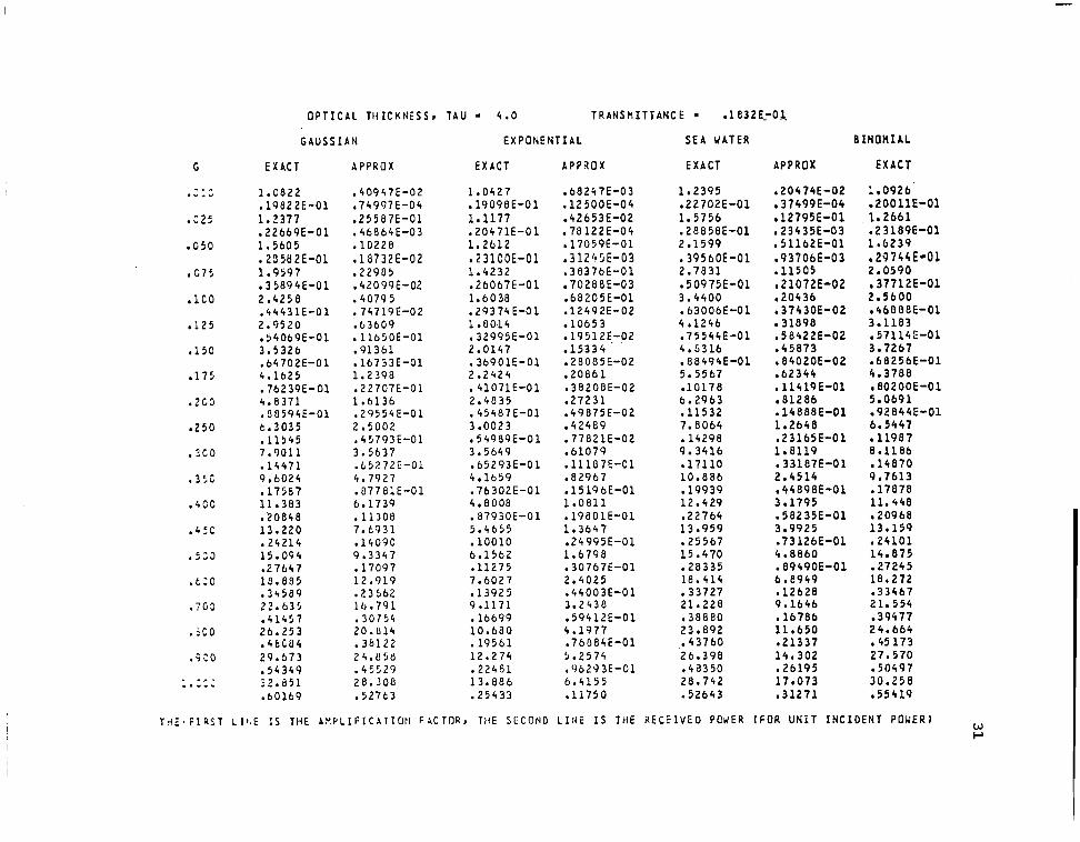
The numerical results presented in Figs. 3 to 7 were obtained from a

relatively simple computer program, consisting of less than 100 executable

statements. A full listing, and partial output, are included in this

appendix.

The task of this program is to evaluate the numerical integrals in

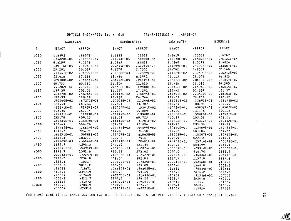
Eqs.' (23), (25d), (27d) and (30'), for a series of values of Is between

0.5 and 15.0, and a series of values of G up to 1.0. For comparison,

the Arnush-Stotts approximation, Eq. (39), is also computed. We have

included the full results for 'c S

values of 4.0 and 10.0, which may be

read in conjunction with Fig. 5.

Although infinite integrals of this type are often handled by

Gauss-Laguerre quadrature, this method was found wanting, due to the

oscillatory nature of the integrand. Instead we have employed Simpson's

rule, up to a finite cut off, allowing for the remainder of the integral

by the following result:

If

fog = @ (xl for x ? X -

and

@(Jo dx = Q is known, 0

then

co X

f(x) dx = Q + [f(x) - G(x) I dx . 0 0

(Al)

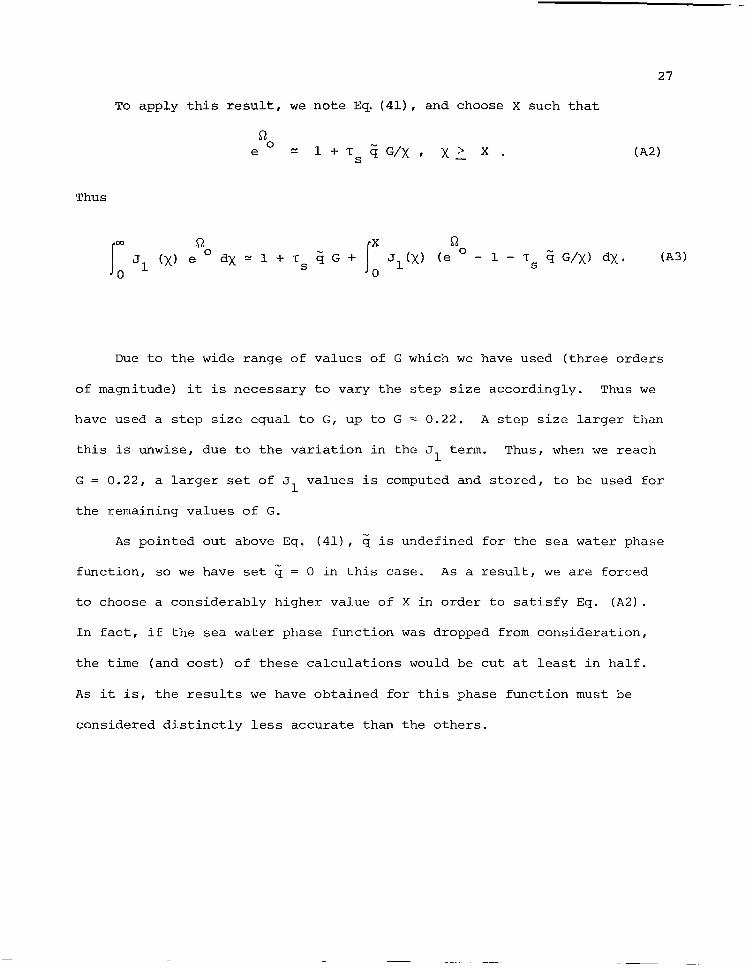
27

To apply this result, we note Eq. (411, and choose X such that

52 0 e = l+IsgG/x, x, X. (A2)

Thus

I

m R

I

X i-2 Jl (x) e odx"l+TsqG+ J,(x) (e"- l-IseG/x) dx. (A3)

0 0

Due to the wide range of values of G which we have used (three orders

of magnitude) it is necessary to vary the step size accordingly. Thus we

have used a step size equal to G, up to G = 0.22. A step size larger than

this is unwise, due to the variation in the Jl term. Thus, when we reach

G = 0.22, a larger set of J 1 values is computed and stored, to be used for

the remaining values of G.

As pointed out above Eq. (41), s is undefined for the sea water phase

function, so we have set e = 0 in this case. As a result, we are forced

to choose a considerably higher value of X in order to satisfy Eq. (A2).

In fact, if the sea water phase function was dropped from consideration,

the time (and cost) of these calculations would be cut at least in half.

As it is, the results we have obtained for this phase function must be

considered distinctly less accurate than the others.

73174 OPT-1 FTH 4.6+452 79106106. 13.32.33

10

15

20

25

30

35

40

C C C C C C

c" C C C C C C C C C C C C C C C C C C C

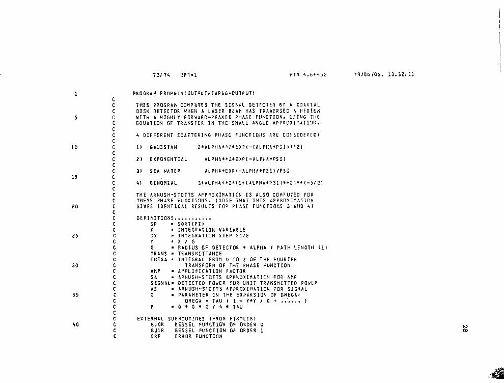
PROGRAM PROPGTN~OUTPUTITAPE~=OUTPUT~

THIS PROGRAM COMPUTES THE SIGNAL DETECTED BY A COAXIAL DISK DETECTOR WHEN A LASER BEAM HAS TRAVERSED A MEDIU'? WITH A HIGHLY FORWARD-PEAKED PHASE FUNCTION, USING TilE EOUATION OF TRANSFER IN THE SMALL ANGLE APPROXIMATION.

4 DIFFERENT SCATTERING PHASE FUNCTIONS ARE COflSIOEPfDI

11 GAUSSIAN 2*ALPHA*;bZ*EXP(-(ALPHA*PSI)""2)

2) EXPONENTIAL ALPHA**2*EXPl-ALPHA*PSIl

31 SEA WATER ALPHA*EXP(-ALPHA+'PSI)/PSI

41 6IN6MIAL 32ALPHA~*2*~1+~ALPHA*PStl*~Z~**~-5/2)

THE ARNUSH-STOTTS At'PROXIflATION IS ALSO COtlPUTED FOR THESE PHASE FUNCTIONS. (NOTE THAT THIS ~PPttoxxt’ATIn~ GIVES IDENTICAL RESULTS FOR PHASE FUtlCTIOflS 3 AtJO 41

DEFINITIONS........... SP = SORT(PI) X = INTEGRATION VARIABLE DX l INTEGRATION STEP SIZE Y . X / G G = RADIUS OF DETECTOR * ALPHA I PATH LENGTH 12) TRANS m TRANSMITTANCE OMEGA * INTEGRAL FROM 0 TO 2 UF THE FOURIER

TRANSFORM OF THE PHASE FUNCTION AMP = AMPLIFICATION FACTOR SA 9 ARNUSH-STOTTS APPROXIAATION FDr'. AMP SIGNALS DETECTED POWER FUR UNIT TRANSMITTED POWER AS l ARNUSH-STOTTS APPROXIMATION FOR SIGNAL 0 l PARAMETER IN THE EXPANSION OF OMEGA:

OflEGA = TAU I 1 - Y*Y / 0 + .:.... 1 P n O*G*G/4'tTAU

EXTERNAL SUPROUTII~ES (FROM FTNMLIB) BJOR BESSEL FUNCTION OF ORDER 0 DJlR BESSEL FUNCTION OF ORDER 1 ERF ERROR FUNCTION

45

50

55

60

65

70

75

80

73174 OPT*1 FTN !+.6+452 79/Ob/Ob. 13.32.:

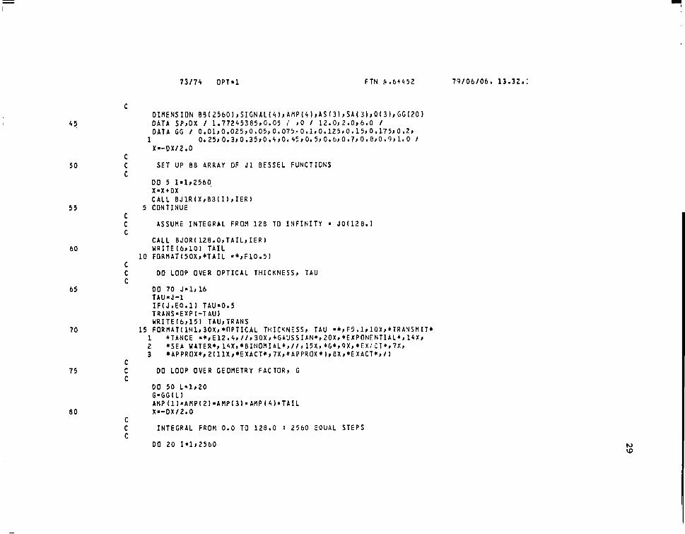
C OIWENSION B9~25b0~,SIGNAL~4~,AHP~4~~AS~31,SA~3),P~3l~GG~ZO~ DATA SP,DX / 1.77245385~0.05 i rQ I 12.0j2.0,b.O / DATA CC / 0.01,0.025~0,05~0.075~0.1~0.125,0.15,0.175~0.2~

1 0.25r0.3,0.35,0.4,0.45,0.5~0.6~0.7r0.e,0.9~1.0 I x~-Dx/z.o

C

: SET UP BB ARRAY OF Jl BESSEL FUNCTIONS

DO 5 I=lr2560, XmXtDX CALL BJ~R(XIBB(I),IER)

5 CONTINUE

c” ASSUME INTEGRAL FROH 128 TO INFINITY ' JO(128.1 C

CALL BJOR(lZB.O,TAIL,IER) WRITE(6,lOl TAIL

10 FDRMAT(SOX,*TAIL **,FlO.S)

i DO LOOP OVER OPTICAL THICKNESS, TAU L

00 70 J=l,lb TAU=J-1 IF(J.EO.11 TAU=O.S TRANS=EXP(-TAU) WRITE(6,151 TAUjTRANS

15 FOR~IAT(~H~,~OXI*OPTICAL THICKNESS, TAU n *,F5.l,lOXr*TR4NSflIl* 1 *TANCE =+,E12.4,//,30X,+GAUSSIAN*~2OX~*EXPDNFNT1AL+~l4X~ 2 *SEA WATER+,14X,*BI~~O~IAL*~//~l5X,*G*~9X~*~X~~l*~7X~ 3 *APPROX*,Z~llX,*EXACT*~7X~~APPROX*~~BX,rEXACl*~/~

L c DO LODP OVER GEDHETRY FACTOR, G C

DO 50 L=l,ZO GmGG(L1 A~P(l)=AHP(Zl=AflP(3~~AMP(4)~TAIL X=-DXI2.0

c” INTEGRAL FROH 0.0 TO 128.0 : 2560 EOUAL STEPS L

DO 20 1*1,2560 hl W

PPOGRAH PROPGTN 73174 OPlml FTN 4.6+452 77JOhlC5. 13.32..

05

90

9s

C 100 C

:

105

110

115

120

X-X+0X t31=90(11 YmXlG CALL EPF(O.S*Y,ERFYl ONEGA~TAU*SP*EQFYIY A'lP~11.AHP~11+B1*EXP(OCEGAl*DX OHEGA~TAUISORTI1.O+YstZ) AHP~2l=AilP~2l+01*EXP~O~EGAI*DX OtlEGA=lAU/Y*ALOG(Y+SORT~l.O+Y**Zll AnP(3)~A~P(3)t31*EXP(ONEGA)~DX UflEGA~Z.O*TAU/Y IF(Y.LT.201 OMEGA=OHEGA-TAU*EXP(-YI*tl.O+Z.O/Yl AMPI4l~AtlP(4I+Bl*EXP~ONEGAl*DX

20 CONTINUE

NOW CALCULATE THE AQNUSH-STOTTS APPROXIMATION (QESULTS FOR PHASE FUNCTIONS 3 t 4 ARE IOENTICALl

DO 25 1~193 P=O~Il*G+G/4.0/TAU ASTIl~l.O-EXPt-Pl SA(Il=AS(II/TRANS SIGNAL(II=ARP(II*TRANS

25 CONTINUE SIGNAL(4l~AMP(41+TRANS WRITE16,301 G~~A~P~1~,SA~I~rl~lr3~rhnP14~

30 FORNAT(llX,F7.3,3(3X,2Gl3.5),C13.5I WRITE(6,35) ~SIGNAL~Il,AS~II,I~1,3),SIGNAL~4I

35 FORNAT~18X>3~3X,2G13.5)rG13.51 50 CONTINUE

WRITE~brbOl 60 FORflAT(/,lOX,*THE FIRST LINE IS THE AflPLIFICATION FACTOR, THE *,

1 *SECOKD LINE IS THE RECEIVED POWER (FOW UNIT INCIOEKT PO;IERl*l 70 CONTINUE

STOP END

OPTICAL THICKNESSI TAU - 4.0 TRANStlITTANCE n .lfJ32E--01

G

. . . .".II

-2: .*

.GSO

.c7:

.lCO

,125

,150

,175

.?CO

,250

.?CO

.35b

.4cc

,.4:c

.::3

.t:0

.:c3

. ice

.iCO

. -r- ..1-1

GAUSSIAN EXPONENTIAL SEA WATER BiNOHIAL

EXACT APPROX EXACT APPROX EXACT APPROX EXACT

1.0822 .19822E-01 1.2377 .22669E-01 1.5605 .235t!ZE-01 1.9597 .35894E-01 2.4250 .44431E-01 2.9520 .54069E-01 3.5326 .64702E-01 4.1625

. 40947E-02

.74997E-04

.25587E-01

1.0427

. 46864E-03

.10228 ,10732E-02 .22905 .42099E-02

40795 :74719E-02 .63609

. 19098E-01 1.1177 .20471E-01 1.2612 .23100E-01 1.4232 .26067E-01 1.6038

. llbSOE-01 .91361 .16733E-01 1.2398 .22707E-01 1.6136 .29554E-01 2.5002 .45793E-01 3.5637 .b5272E-01 4.7927

. 29374E-01 1.80.14 .32995E-01 2.0147 .36901E-01 2.2424

. 76239E-01 4.0371 .90594E-01 t.3035 .11545 7.9011 .14471 9.6024 .17587 11.383 .20848 13.220 .24214 15.094 .27647 18.085 .3+509 22.635 .41457 26.253 .4hL04 29.673 .54349 32.a51 .60169

. 1?77elE-01 6.1739 .11308 7.t931 a14090 9.3347 .17097 12.919 .23662 16.791 .30754 20.U14

. 41071E-01 2.4035

45487E-01 i.0023 .549896-01 3.5649 .65293E-01 4.1659 .76302E-01 4.8008

.68247E-03

.12500E-04

.42653E-02 .78122E-04 .17059E-01 .312'r5E-03 .30376E-01 .70288E-03 .68205E-01 .12492E-02 .10653 .19512E-02 l 15334' .28085E-02 .20861 .38208E-02 .27231 .49075E-02 .42409

. 3b122 24.U5tl .4::20 28.308 .S2763

. 87930E-01 5.4655 .lOOlO 6.1562 .11275 7.6027 .13925 9.1171 .16699 10.6ao .19561 12.274 .22481 13.886 .25433

. 77821E-02

.61079

.11107E-01

.02967

.15196E-01 1.0811 .19801E-01 1.3647 .24995E-01 1.6798 .30767E-01 2.4025 .44003E-01 3.2430 .59412E-01 4.1977 .76084E-01 5.2574 .96233E-01 6.4155 .11750

1.2395 .22702E-01 1.5756 .28858E-01 2.1599 .395bOE-01 2.7831 .50975E-01 3.4400 .63006E-01 4.1246 .75544E-01 4.6316 .88494E-01 5.5567 .10178 6.2963 .11532 7.8064 .14298 9.3416 .17110 10.886 .19939 12.429 .22764 13.959 .25567 15.470 .28335 18.414 .33727 21.228 .38880 23.092 ,.43760 26.390 .48350 28.742 .52643

.20474E-02

.37499E-04

.12795E-01

.23435E-03

.51162E-01 .9370bE-03 .11505 .21072E-02 .20436 .37430E-02 .31398 .58422E-02 .45873 .84020E-02 .62344 .11419E-01 .8128b .14888E-01 1.2648 .231bSE-01 1.8119 .33187E-01 2.4514 .44898E-01 3.1795 .58235E-01 3.9925 .7312bE-01 4 .a860 .89490E-01 6.0949 .12628 9.1646

16786 il.650 .21337 14.302 .26195 17.073 .31271

:.D92b .20011E-01 1.2bbl .23189E-01 1.6239 .23744E=Ol 2.0590 .37712E-01 Z.JbOO .46008E-01 3.1183 .57114i-01 3.7267 .6825bE-01 4.3780 .80200E-01 5.0691 .92044E-01 b.5447 .11987 8.1186 a14870 9.7613 .17070 11.448 .20968 13.159 .24101 14.875 .27245 18.272 .33467 21.554 .39477 24.664 .45173 27.570 .50497 30.258 .55419

Trl.FIRST LI'sE IS THE Ab'.PLIFIChTIO~l FACTOR> THE SCCOND LIfiE IS THE RECEIVED PCdER (FOR UtiiT INCIDENT POKER) E

G

.OlO

.025

,050

,075

,100

.125

.150

.175

.200

,250

,300

.350

,400

.450

,500

,600

,700

,800

,900

l,.OOO

OPTICAL THICKNESS, TAU l 10.0 TRANSHITTANCE . ,4540E-04

GAUSS IAN

EXACT

1.6482 .7482BE-04 8.6159 .3911bE-03 25.201 .11441E-02 52.616 .23BBBE-02 90.753 .41202E-02 139.38 .b3278E-02 198.33 .9004OE-02 267.43 .12141E-01 346.50 .15731E-01 533.70 .24234E-01 750.49 .34435E-01 1018.7 .4625 lE-01 1312.5 .59589E-01 1637.7 .74350E-01 1991.9 .90432E-01 2770.2 .12613 3652.2 .16581 4594.5 .20859 5506.3 .25362 6609. b *30007

APPROX

.bb078

.30000E-04 4.1296 .1874BE-03 lb.514 .74972E-03 37.138 . IbBblE-02 65.980 .29955E-02 103.01 L 46765E-02 148.18 .67273E-02 201.44 .91454E-02 262.74 .11928E-01 409.15 .18575E-01 506.76 .26639E-01 794.70 .36083E-01 1032.3 . 468 bbE-01 1298.3 .58942E-01 1591 .b .72257E-01 2254.9 .10237 3011.2 .13671 3047.9 .I7469 4751.7 .21573 5706.9 .25918

EXPONENTIAL

EiACT APPROX

1.1333 .11013 .51453E-04 .50000E-05 2.0765 .68032 .94274E-04 .31250E-04 7.1070 2.7531 .322bbE-03 .12499E-03 13.436 6.1941 .6099OE-03 .20121E-03 21.204 .962bbE-03 31.087 .14113E-02 43.167 .19598E-02' 57.393 .2605bE-02 73.724 .33471E-02 112.59 .5lllbE-02 159.59 .?2454E-02 214.56 .97409E-02 277.33 .12591E-01

11.010 .4990BE-03 17.201 .78094E-03 24.766 .11244E-02 33.702 .15301E-02 44.009 .19900E-02 60.725 . 31201E-02 90.096 . 44899E-02 134.50 .61063E-02 175.51 .79681E-02

347.75 221.09 .15788E-01 .100?4E-01 425.63 273.62 .19323E-01 .12422E-01 603.05 392.93 .27370E-01 .1?839E-01 808.09 533.c9 .3668?E-01 .24202E-01 1039.2 693.69 .47170E-01 .31493E-01 1294.6 074.25 .50?7?E-01 .39091E-01 1572.0 1074.2 ,71407E-01 .48771E-01

SEA WATER BI!iOMlAL

EXACT APPROX EXACT

2.2419 .33039 1.6767 .lOl?OE-03 .15000E-04 .76123i-C4 0.5240 2.0649 7.4024 .30699E-03 .9374bE-04 .3?607E-C3 25.702 0.2504 22.560 .llbb9E-02 .37493E-03 .10242!-02 51.115 10.577 46.3?5 .23206E-02 .04339E-03 .210:7E-C2 05.476 33.015 73.335 .3BEObE-02 .14989E-02 .36045E-G2 128.42 51.564 121.37 .50301E-02 .23410E-02 .55103E-02 179.57 74.214 172.12 .0152bE-02 .33693E-02 .?31kZf-Ci 238.63 100.95 . 231.44 .10834E-01 .45832E-02 .1050!E-01 305.29 131.76 299.15 .1306OE-01 .59020E-02 .13581E-01 460.27 205.53 453.Eb .2009bE-01 .93312E-02 .23?32E-Cl 642.20 295.36 649.53 .2316OE-01 .13409E-01 .29;3ei-cl 849.20 401.04 0t9.27 .30553E-01 .10207E-01 .39465E-01 1070.9 522.34 1116.1 .48903E-01 .23714E-01 .SCi?ZE-Cl 1329.5 658.99 1338.1 .60359E-01 .2991BE-01 .63’JZOE-01 1599.0 810.70 1683.2 .?2594E-01 .3bOObE-01 . ?bilbE-01 2187.4 1157.9 2334.3 .99310E-01 .5256eE-01 a 1059t 2C30.h 1560.9 3053.2 .12051 , ?0864E-01 .13361 3515.9 2016.2 3e24.3 .15962 .9153bE-01 . l?!ki 4232.4 2520.0 4t33 .i .19z15 .11441 . .- 1 2 f 4 4970.1 3068.1 '5 4 : '5 . .I .22564 .13929 .2i31!

7HE FIRST LINE IS THE AMPLIFICATION FACTOR , THE SECOND LINE IS THE PECElVED PI;kEq (FOP: 'J?(IT IhCI;'hT ::.$:I

33 REFERENCES

1. S. Chandrasekhar: "Radiative Transfer," Dover, 1960.

2. L. S. Dolin; Scattering of a Light Beam in a Layer of a Cloudy Medium, Izv. VUZ. Radiofizika, 1 (1964), 380-382.

3. G. Wentzel, Ann. Phys., 69 (19221, 335-345. -

4. H. S. Snyder and W. T. Scott; Multiple Scattering of Fast Charged Particles, Phys. Rev., 76 (1949) 220-225. -

5. W. T. Scott; The Theory of Small-Angle Multiple Scattering of Fast Charged Particles; Rev. Mod. Phys., 35 (1963) 231-313. -

6. D. M. Bravo-Zhivotovskiy, L. S. Dolin, A. G. Luchinin and V. A. Savel'yev; Structure of a EJarrow Light Beam in Sea Water, Izv. Atmos. Oceanic Phys., 5 (1969) 160-167. -

7. W. G. Tam and A. Zardecki; Laser Beam Propagation in Particulate Media; J. Opt. Sot. Am., 69 (1979) 68-70.

8. L. S. Dolin; Propagation of a Narrow Beam of Light in a Medium with Strongly Anisotropic Scattering, Izv. VUZ, Radiofizika, _ 9 (1966) 61-71.

9. R. L. Fante; Propagation of Electromagnetic Waves Through Turbulent Plasma Using Transport Theory, IEEE A & P, 21 (1973) 750-755. -

10. D. Arnush; Underwater Light Beam Propagation in the Small-Angle-Scattering Approximation, J. Opt. Sot. Am., 62 (1972) 1109-1111.

11. L. B. Stotts; The Radiance Produced by Laser Radiation Transversing a Particulate Multiple-Scattering Medium, J. Opt. Sot. Am., 67 (1977) - 815-819.

12. L. B. Stotts; Limitations of Approximate Fourier Techniques in Solving Radiative-Transfer Problems, J. Opt. Sot. Am., 69, (1979) 1719-1723.

13. W. G. Tam and A. Zardecki; Multiple Scattering of a Laser Beam by Radiational and Advective Fogs; Optica Acta, _ 26 (1979), 659-670.

34

I0.l

I.C

0.1

0.01

0.001

i I

‘F-SEA WATER: P=a 9-l ;“*,2* \

\ \

\ \ ‘Y

A,“ \

\

0.0 0.5 1.0 1.5 2.0 2.5 30 3.5

arlr

FIGURE 1. Normalized phase functi'on p vs a* for four model phase

functions.

1.0

0.4

0.1

km

2 0.04

0.01

0.004

. . . . . . . . . . . . . . . . . .

. . .

EXACT APPROACH USING PHASE FUNCTIONS

- GAUSSIAN - - - BINOMIAL - - - MPONENTIAL -------. SEA WATER

. . . . . ARNUSH - STOTTS APPROXI MATION

0.4 1.0 4.0 10.0 40.0 100.0 400.0 l000.0

Y

FIGURE 2. fio/Ts vs. y for four model phase functions and for the Amush-Stotts

approximation.

36

FIGURE 3.

phase function.

v 0.1 0.2 0.3 0.4 0.5 06 0.7

GEOMETRY FACTOR, G

Amplification factor A vs. geometry factor G for the Gaussian

2 4 6 8 IO 12 14

SCATTERING OPTICAL THICKNESS, rS

37

5 \ \

TRANSMISSION

FIGURE 4. Normalized power received vs. scattering optical thickness

for the Gaussian phase function.

38

INS EXACT APPROACH USING PHASE FUNCTIONS

--- BINOMIAL --- EXPONENTIAL --------. SEA WATER

. * *. *ARNUSH - STOTTS APPROXIMATION

0.5 0.6 0.7

FIGURE 5. Amplification factor A vs. geometry factor

of T and four model phase functions for our approach and S

approxima ti on.

G for two values

the Arnush-Stotts

39

2.0

1.0

0.5

0.2

0 0.1

2

4 0.05

0.02

0.01

0.05

EXACT APPROACH USING PHASE FUNCTIONS GAUSSI AN

- - - BINOMIAL --- EXPONENTIAL --------- SEA WATER

r

0.005 0.01 0.02 0.05

G 0.1 0.2 0.5 1.0

FIGURE 6. Subtracted amplification factor (A - 1.0) vs. geometry

factor (G) for 'I = 1.0.

50

20

IO

5

2

I

0 2

lx 0.5

0.2

0.1

0.05

0.02

0.01

40

EXACT APPROACH USING PHASE FUNCTIONS

- GAUSSIAN -- - BINOMIAL --- EXPONENTIAL --------- SEA WATER

........ ARNUSH - STOTTS APPROXIMATION

FIGURE 7. Subtracted amplification factor (A - 1.0) vs. geometry

factor (G) for T = 5.0.

1. REPORT NO. 2. GOVERNMENT ACCESSION NO. 3. RECIPIENT’S CATALOG NO.

NASA ,CR-3407 4. TITLE AND SUBTITLE 5. REPORT DATE

Small-Angle Approximation to the Transfer of Narrow Laser April 1981 Beams in Anisotropic Scattering Media 6. PERFORMING ORGANIZATION CODE

7. AUTHOR(S)

Michael A. Box* 8. PERFORMING ORGANIZATION REPDR’T

and Adarsh Deepak 9. PERFORMING ORGANIZATION NAME AND ADDRESS 10. WORK UNIT, NO.

Institute for Atmospheric Optics and Remote Sensing M-345 P-0. Box P 11. CONTRACT OR GRANT NO.

Hampton, Virginia 23666 NAS8-33135 13. TYPE OF REPOR-; & PERIOD COVERE

12. SPONSORING AGENCY NAME AND ADDRESS

National Aeronautics and Space Administration Contractor Report

Washington, D.C. 20546 14. SPONSORING AGENCY CODE

IS. SUPPLEMENTARY NOTES * Present Affiliation: Institute of Atmospheric Physics, University of Arizona,

Tucson, Arizona 85721 Marshall Contract Monitor: B. J. Anderson

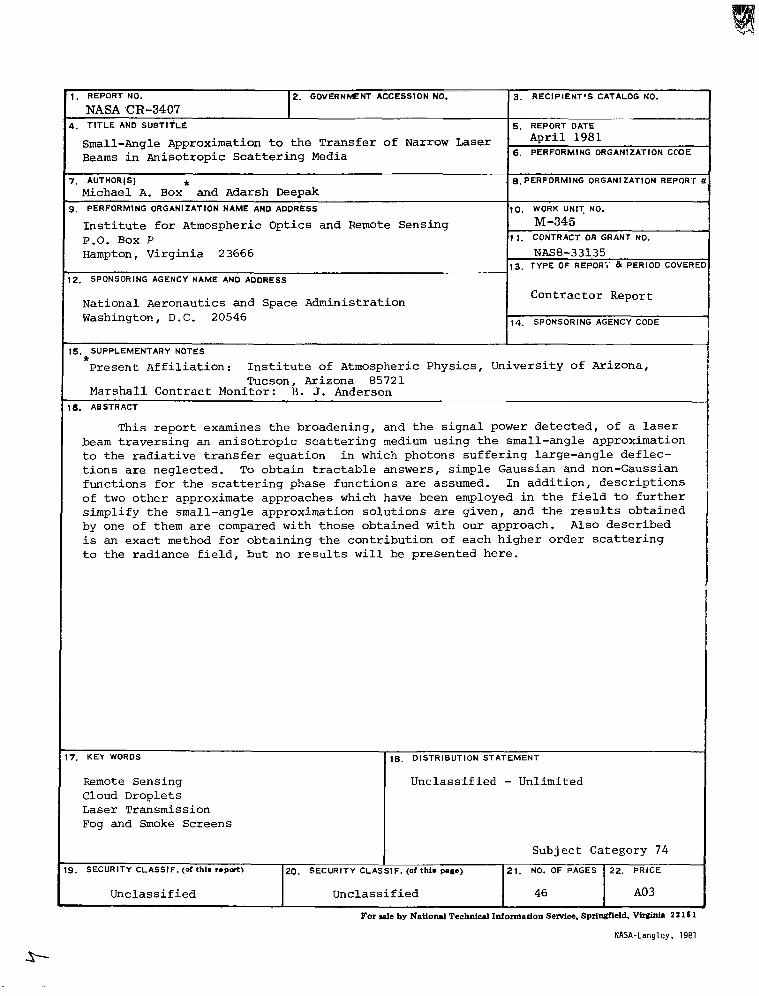
16. ABSTRACT

This report examines the broadening, and the signal power detected, of a laser beam traversing an anisotropic scattering medium using the small-angle approximation to the radiative transfer equation in which photons suffering large-angle deflec- tions are neglected. To obtain tractable answers, simple Gaussian and non-Gaussian functions for the scattering phase functions are assumed. In addition, descriptions of two other approximate approaches which have been employed in the field to further simplify the small-angle approximation solutions are given, and the results obtained by one of them are compared with those obtained with our approach. Also described is an exact method for obtaining the contribution of each higher order scattering to the radiance field, but no results will be presented here.

7. KEY WORDS

Remote Sensing Cloud Droplets Laser Transmission Fog and Smoke Screens

18. DISTRIBUTION STATEMENT

Unclassified - Unlimited

Subject Category 74 3. SECURITY CLASSIF. (of thlm r.port, 20. SECURITY CLASSIF. (of this pale) 21. NO. OF PAGES 22. PRICE

Unclassified Unclassified 46 A03

For sale by Nationd Technical Information Service. Spdnefield. Vtihh 2 116 1

NASA-Lang1 ey, 1981