Embed Size (px)
Citation preview
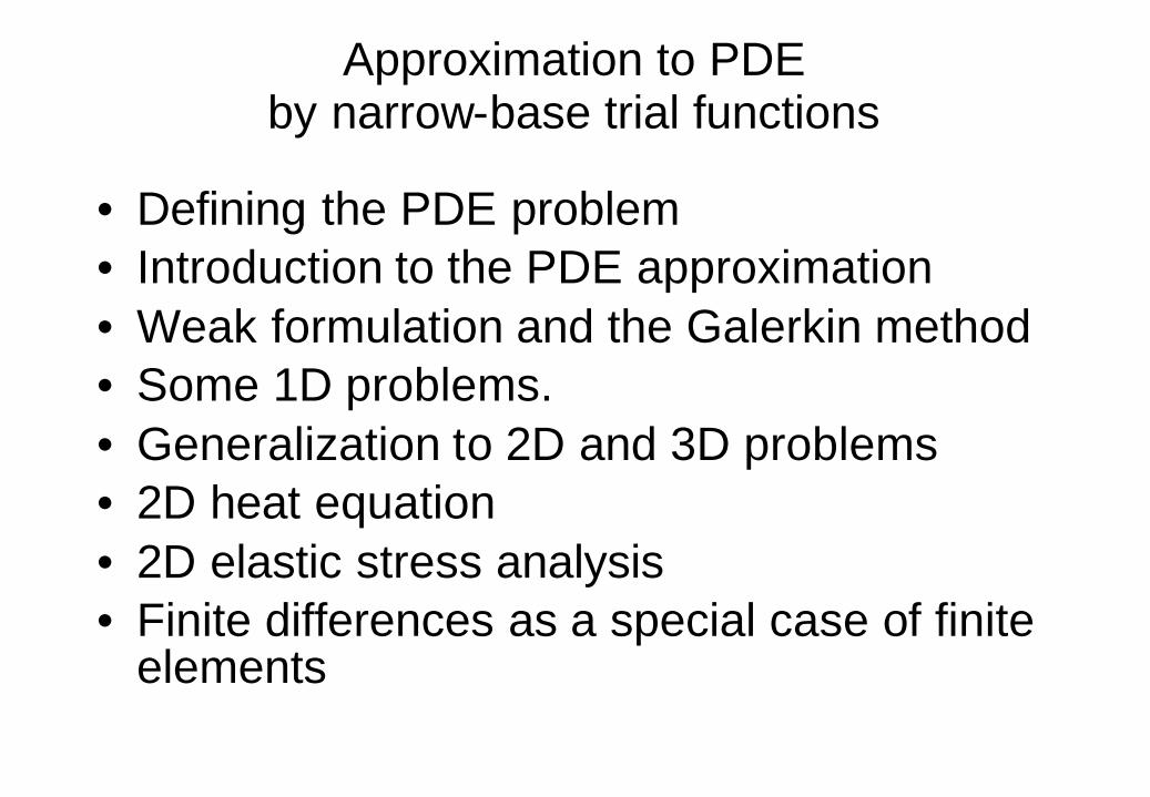
Approximation to PDEby narrow-base trial functions
• Defining the PDE problem• Introduction to the PDE approximation• Weak formulation and the Galerkin method• Some 1D problems.• Generalization to 2D and 3D problems• 2D heat equation• 2D elastic stress analysis• Finite differences as a special case of finite
elements
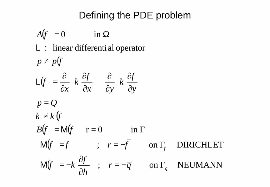
Defining the PDE problem
( )
( )
( )
( )( ) ( )
( )
( )
Γ−=∂∂
−=
Γ−==
Γ=+=≠=
∂∂
∂∂
+
∂∂
∂∂
=
≠
Ω=
NEUMANN on ;
DIRICHLET on ;
in 0r
operator aldifferentilinear in 0
qqr
r
B
Qp
yyxx
pp
A
ηφ
κφ
φφφ
φφφκκ
φκ
φκφ
φ
φ
φ
M
M
M
L
: L
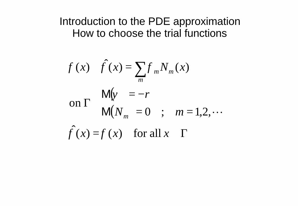
Introduction to the PDE approximationHow to choose the trial functions
( )( )
Γ∈=
==−=
Γ
=≅ ∑
xxx
mNr
xNxx
m
mmm
allfor )()(ˆ
,2,1;0 on
)()(ˆ)(
φφ
ψ
φφφ
LMM
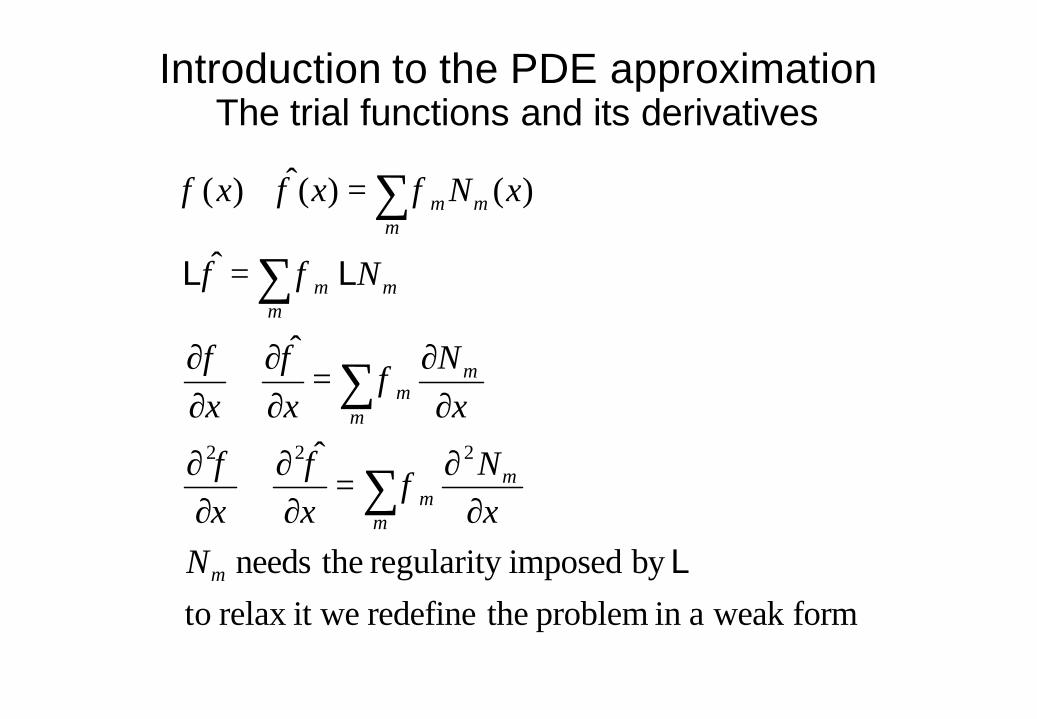
Introduction to the PDE approximationThe trial functions and its derivatives
form weak ain problem theredefine it werelax toby imposed regularity theneeds
ˆ
ˆ
ˆ
)()(ˆ)(
222
L
LL
m
m
mm
m
mm
mmm
mmm
NxN
xx
xN
xx
N
xNxx
∑
∑
∑
∑
∂∂
=∂∂
≅∂
∂
∂∂
=∂∂
≅∂∂
=
=≅
φφφ
φφφ
φφ
φφφ
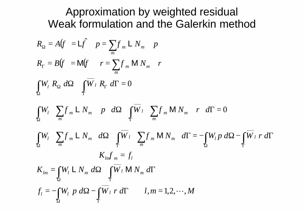
Approximation by weighted residualWeak formulation and the Galerkin method
( )
( ) ( )
MmldrWdpWf
dNWdNWK
fK
drWdpWdNWdNW
drNWdpNW
dRWdRW
rNrBR
pNpAR
lll
mlmllm
lmlm
llm
mmlm
mml
mmml
mmml
ll
mmm
mmm
,,2,1,
0
0
ˆ
L=Γ−Ω−=
Γ+Ω=
=
Γ−Ω−=Γ
+Ω
=Γ
++Ω
+
=Γ+Ω
+=+==
+=+==
∫∫
∫∫
∫∫∑∫∑∫
∑∫∑∫
∫∫
∑
∑
ΓΩ
ΓΩ
ΓΩΓΩ
ΓΩ
ΓΓ
ΩΩ
Γ
Ω
ML
ML
ML
MM
LL
φ
φφ
φφ
φφφ
φφφ
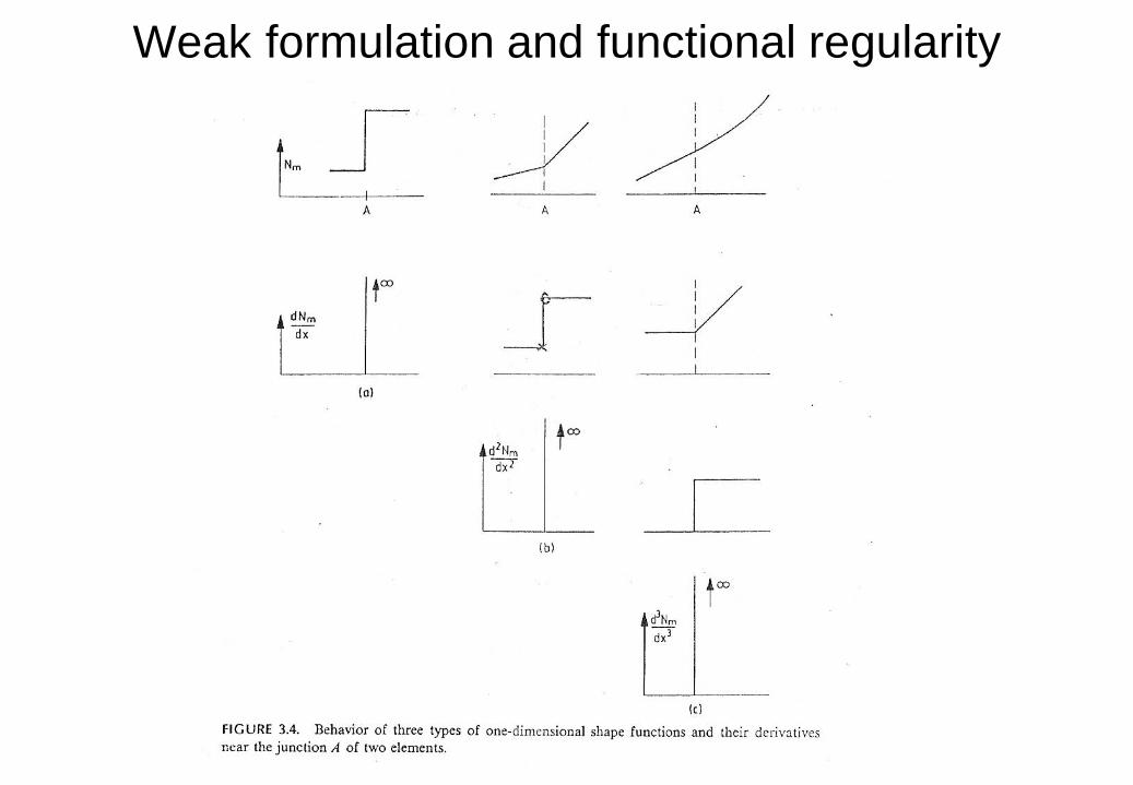
Weak formulation and functional regularity
Weak formulation and functional regularity
( )
( ) ( )( )
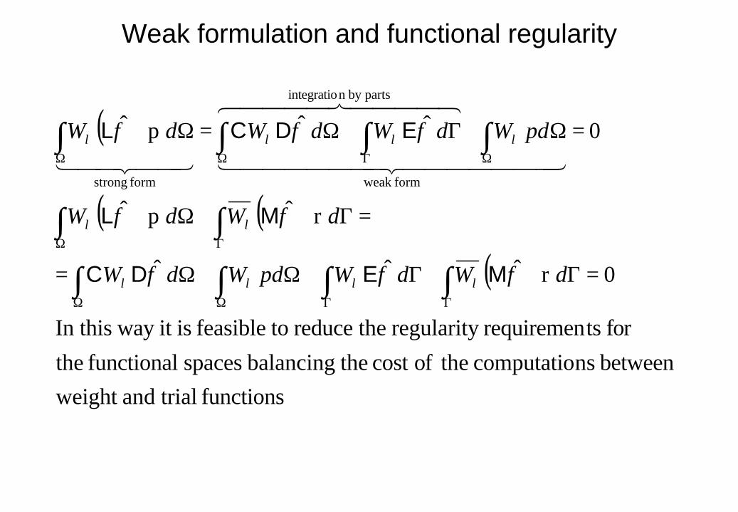
functions trialandweight between nscomputatio theofcost thebalancing spaces functional the
for tsrequiremen regularity thereduce tofeasible isit way In this
0rˆˆˆ
rˆpˆ
0ˆˆpˆ
formweak
partsby n integratio
form strong
=Γ++Γ+Ω+Ω=
=Γ++Ω+
=Ω+Γ+Ω=Ω+
∫∫∫∫
∫∫
∫∫∫∫
ΓΓΩΩ
ΓΩ
ΩΓΩΩ
dWdWpdWdW
dWdW
pdWdWdWdW
llll
ll
llll
φφφ
φφ
φφφ
MEDC
ML
EDCL4444444 34444444 21
4444 84444 76
44 344 21
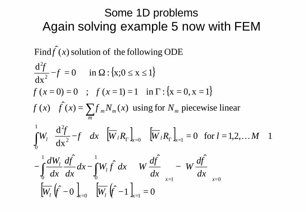
Some 1D problemsAgain solving example 5 now with FEM
[ ] [ ]
( )[ ] ( )[ ] 01ˆ0ˆ
ˆˆˆ
ˆ
1,2,1for 0dxd
linear piecewise for using )()(ˆ)(
1x0,x:in 1)1(;0)0(
1xx;0:in 0dxd
ODE following theofsolution )(ˆ Find
10
01
1
0
1
0
10
1
02
2
2
2
=−+−+
+
−
+−−
+==++
−
=≅
==Γ====
≤≤Ω=−
==
==
=Γ=Γ
∫ ∫
∫
∑
xlxl
xx
ll
xlxll
mm
mm
WW
dxd
Wdxd
WdxWdxdxd
dxdW
MlRWRWdxW
NxNxx
xx
x
φφ
φφφ
φ
φφ
φφφ
φφ
φφ
φ
K
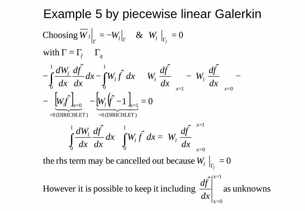
Example 5 by piecewise linear Galerkin
[ ] ( )[ ]
unknowns asˆ
includingit keep topossible isit However
0 becauseout cancelled bemay termrhs the
ˆˆ
ˆ
01ˆˆ
ˆˆˆ
ˆ
with
0 & Choosing
1x
0x
1
0
1
0
1
0
)(DIRICHLET 0
1
)(DIRICHLET 0
0
01
1
0
1
0
=
=
Γ
=
=
=
=
=
=
==
ΓΓΓ
=
=+⇒
=−−−
−
−
+−−
Γ∪Γ=Γ
=−=
∫ ∫
∫ ∫
dxd
W
dxd
WdxWdxdxd
dxdW
WW
dxd
Wdxd
WdxWdxdxd
dxdW
WWW
l
x
x
lll
xlxl
x
l
x
lll
q
lll
φ
φφ
φ
φφ
φφφ
φ
φ
φ
φ
4342143421
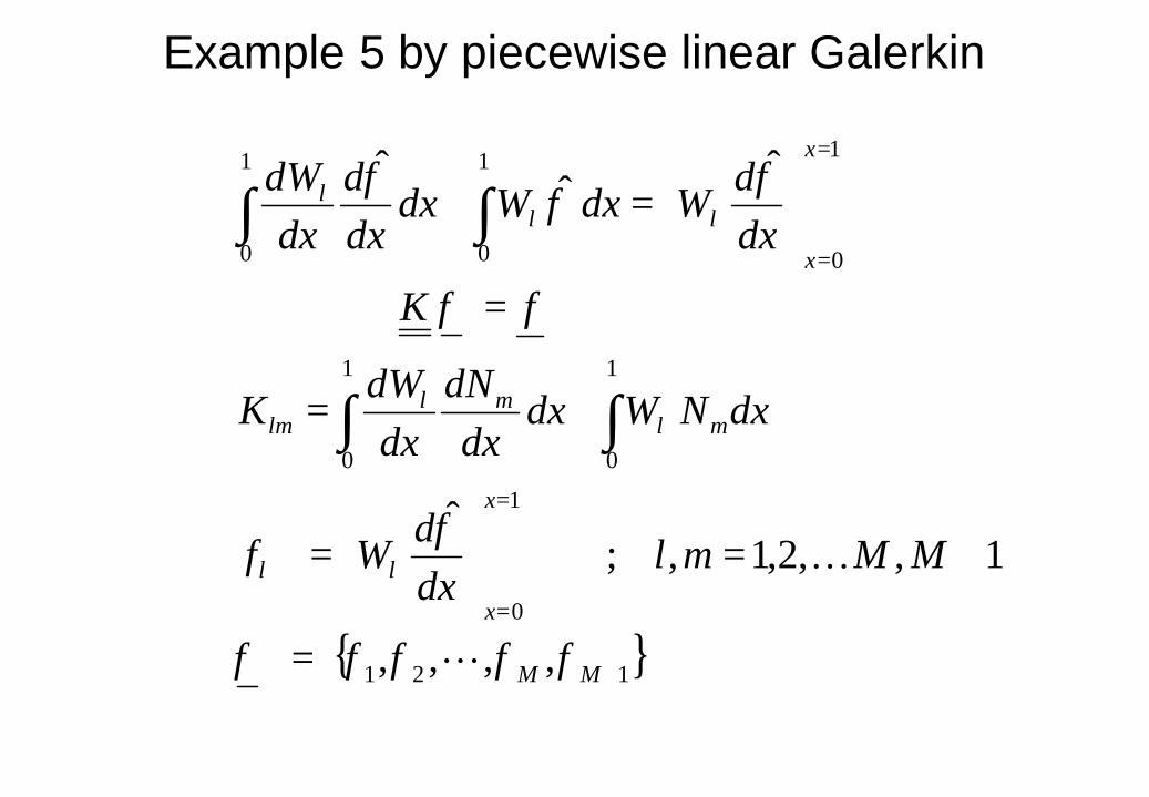
Example 5 by piecewise linear Galerkin
121
1
0
1
0
1
0
1
0
1
0
1
0
,,,,
1,,2,1,;ˆ
ˆˆ
ˆ
+
=
=
=
=
=
+=
=
+=
=⇒
=+
∫ ∫
∫ ∫
MM
x
x
ll
mlml
lm
x
x
lll
MMmldxd
Wf
dxNWdxdx
dNdx
dWK
fK
dxd
WdxWdxdxd
dxdW
φφφφφ
φ
φ
φφ
φ
L
K
Example 5 by piecewise linear Galerkin
( )
+=
=
+
==
+−=
=
+==
∉
==
−=−==−
=
∫
∫
∑=
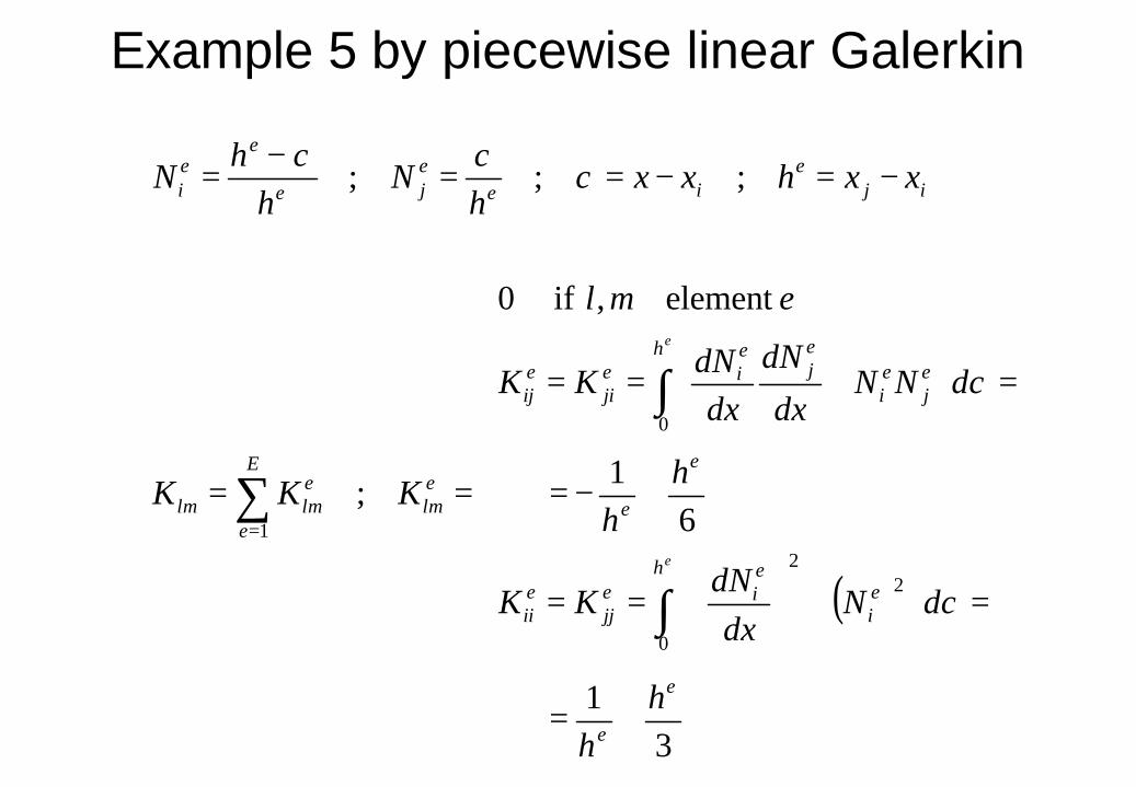
31
61
element , if 0
;
;;;
0
22
0
1
e
e
hei
eie
jjeii
e
e
hej
ei
ej
eie
jieij
elm
E
e
elmlm
ije
ieeje
eei
hh
dNdx
dNKK
hh
dNNdx
dN
dxdN
KK
eml
KKK
xxhxxh
Nh
hN
e
e
χ
χ
χχχ
Example 5 by piecewise linear Galerkin
[ ]
++
++−
+−++
++−
+−++
++−
+−+
=⇒
==
dxd
dxd
dxd
dxd
hh
hh
hh
hhh
hh
h
hh
hhh
hh
h
hh
hh
K
fK
xx
e
e
e
e
e
e
e
ee
e
e
e
e
e
e
ee
e
e
e
e
e
e
e
432
132
3 ELEMENT
12 ELEMENT
1 ELEMENT
0
3 ELEMENT2 ELEMENT1 ELEMENT
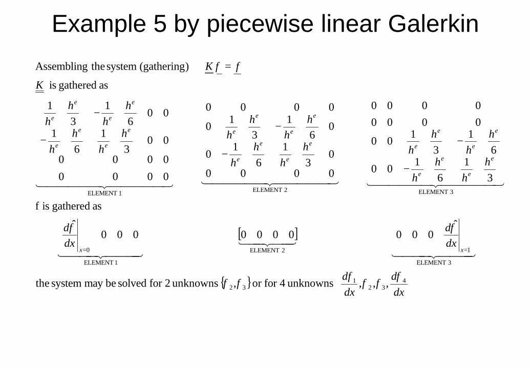
,,, unknowns 4for or , unknowns 2for solved bemay system the
ˆ0000000000
ˆ
as gathered is f
31
61
00
61
31
00
00000000
0000
03
16
10
06
13
10
0000
0000
0000
003
16
1
006
13
1
as gathered is
)(gathering system theAssembling
φφφ
φφφ
φφ
φ
444 3444 214434421
444 3444 21
44444 344444 2144444 344444 2144444 344444 21
Example 5 by piecewise linear Galerkin
=
=
++−
+−+=
−
+−=
++−
+−
+
−
=
=
=
++−
+−
++−
+−
++−
+−+
1
0
31
61
00
006
13
1
and
61
0
31
26
16
13
12
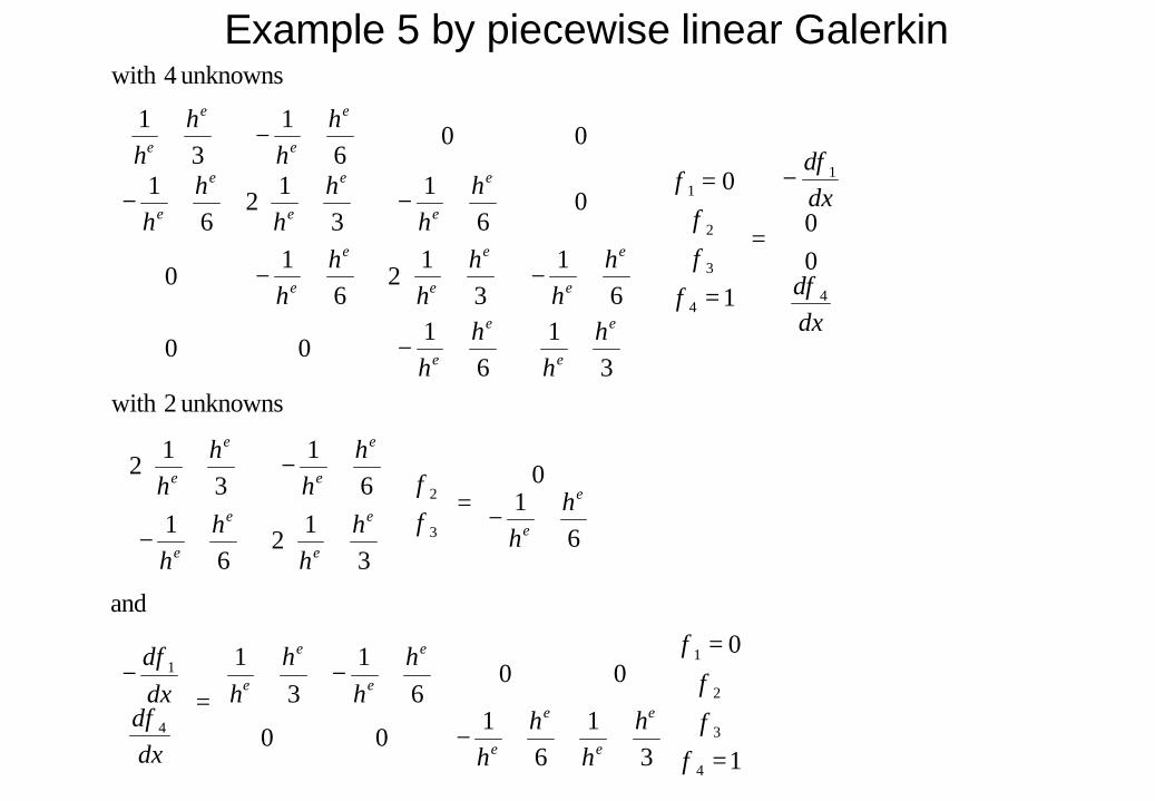
unknowns 2with
00
1
0
31
61
00
61
31
26
10
06
13
12
61
006
13
1
unknowns 4with
4
3
2
1
4
1
3
2
4
1
4
3
2
1
φφφ
φ
φ
φ
φφ
φ
φ
φφφ
φ
e
e
e
e
e
e
e
e
e
ee
e
e
e
e
e
e
e
e
e
e
e
e
e
e
e
e
e
e
e
e
e
e
e
e
e
e
e
hh
hh
hh
hh
dxd
dxd
hhh
hh
h
hh
hh
dxd
dxd
hh
hh
hh
hh
hh
hh
hh
hh
hh
hh
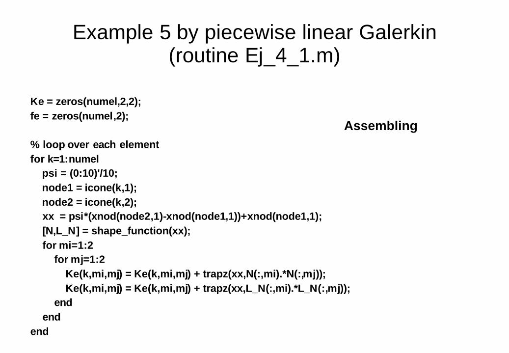
Example 5 by piecewise linear Galerkin(routine Ej_4_1.m)
Ke = zeros(numel,2,2);fe = zeros(numel,2);
% loop over each elementfor k=1:numel
psi = (0:10)'/10; node1 = icone(k,1);node2 = icone(k,2);xx = psi*(xnod(node2,1)-xnod(node1,1))+xnod(node1,1); [N,L_N] = shape_function(xx); for mi=1:2
for mj=1:2Ke(k,mi,mj) = Ke(k,mi,mj) + trapz(xx,N(:,mi).*N(:,mj));Ke(k,mi,mj) = Ke(k,mi,mj) + trapz(xx,L_N(:,mi).*L_N(:,mj));
endend
end
Assembling
Example 5 by piecewise linear Galerkin (routineEj_4_1.m)
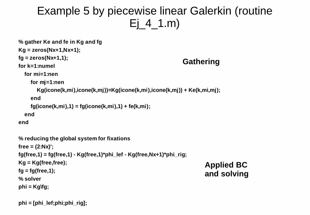
% gather Ke and fe in Kg and fgKg = zeros(Nx+1,Nx+1);fg = zeros(Nx+1,1);for k=1:numel
for mi=1:nenfor mj=1:nen
Kg(icone(k,mi),icone(k,mj))=Kg(icone(k,mi),icone(k,mj)) + Ke(k,mi,mj); endfg(icone(k,mi),1) = fg(icone(k,mi),1) + fe(k,mi);
endend
% reducing the global system for fixationsfree = (2:Nx)';fg(free,1) = fg(free,1) - Kg(free,1)*phi_lef - Kg(free,Nx+1)*phi_rig;Kg = Kg(free,free);fg = fg(free,1);% solverphi = Kg\fg;
phi = [phi_lef;phi;phi_rig];
Gathering
Applied BCand solving
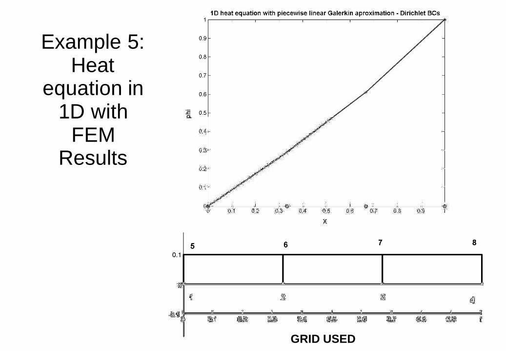
Example 5: Heat
equation in 1D with
FEMResults
GRID USED
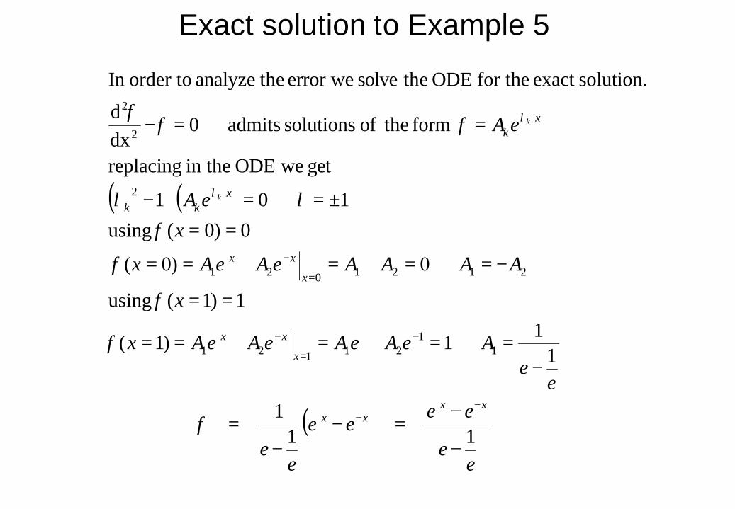
Exact solution to Example 5
( ) ( )
( )e
e
eeee
ee
ee
AeAeAeAeAx
x
AAAAeAeAx
x
eA
eA
xxxx
x
xx
x
xx
xkk
xk
k
k
111
1
11)1(
1)1( using
0)0(
0)0( using
10 1
get weODE in the replacing
form theof solutions admits 0dxd
solution.exact for the ODE thesolve error we theanalyze order toIn
11
21121
2121021
2
2
2
−
−=−
−=∴
−=⇒=+=+==
==
−=⇒=+=+==
==±=⇒=−
==−
−−
−
=
−
=
−
φ
φ
φ
φ
φλλ
φφφ
λ
λ
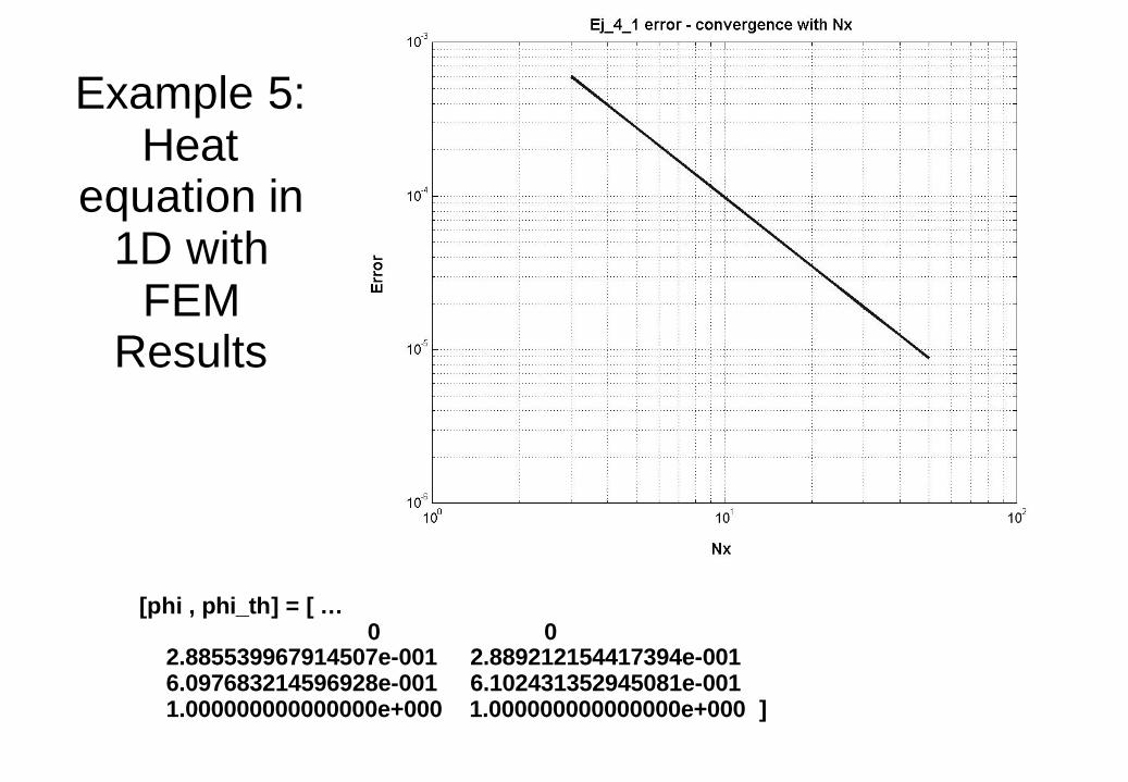
Example 5: Heat
equation in 1D with
FEMResults
[phi , phi_th] = [ …0 0
2.885539967914507e-001 2.889212154417394e-0016.097683214596928e-001 6.102431352945081e-0011.000000000000000e+000 1.000000000000000e+000 ]
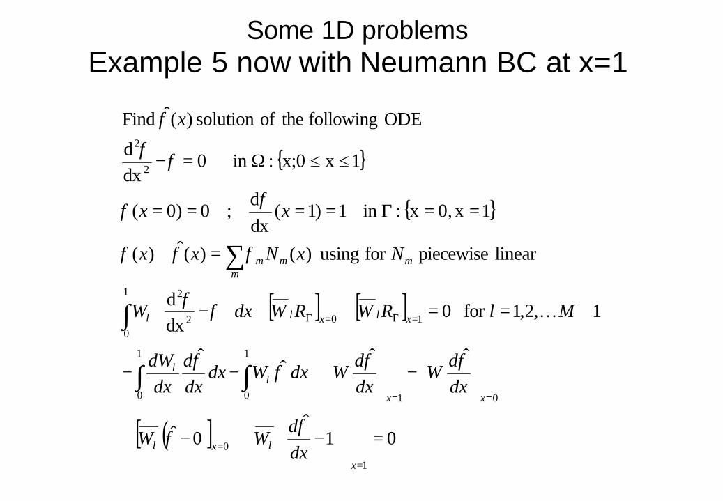
Some 1D problemsExample 5 now with Neumann BC at x=1
[ ] [ ]
( )[ ] 01ˆ
0ˆ
ˆˆˆ
ˆ
1,2,1for 0dxd
linear piecewise for using )()(ˆ)(
1x0,x:in 1)1(dxd
;0)0(
1xx;0:in 0dxd
ODE following theofsolution )(ˆ Find
1
0
01
1
0
1
0
10
1
02
2
2
2
=
−+−+
+
−
+−−
+==++
−
=≅
==Γ====
≤≤Ω=−
=
=
==
=Γ=Γ
∫ ∫
∫
∑
x
lxl
xx
ll
xlxll
mm
mm
dxd
WW
dxd
Wdxd
WdxWdxdxd
dxdW
MlRWRWdxW
NxNxx
xx
x
φφ
φφφ
φ
φφ
φφφ
φφ
φφ
φ
K
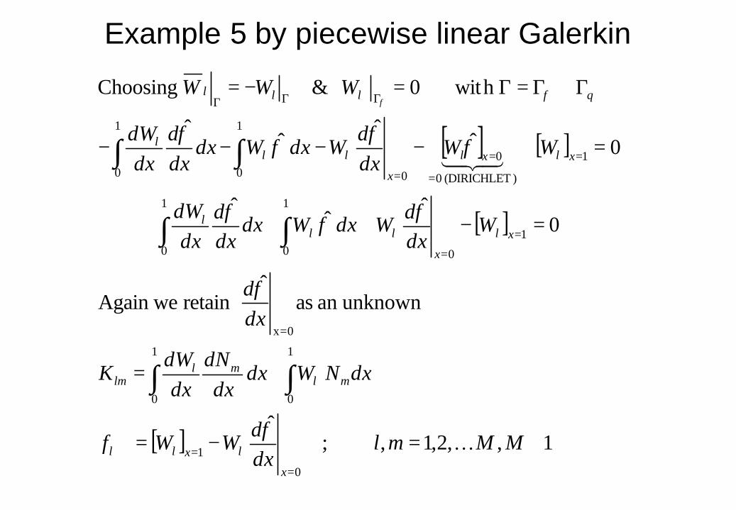
Example 5 by piecewise linear Galerkin
[ ] [ ]
[ ]
[ ] 1,,2,1, ;ˆ
unknownan asˆ
retain Again we
0ˆ
ˆˆ
0ˆˆ
ˆˆ
h wit0 & Choosing
0
1
1
0
1
0
0x
1
0
1
0
1
0
1
)(DIRICHLET 0
0
0
1
0
1
0
+=−=
+=
=−++⇒
=+−−−−
Γ∪Γ=Γ=−=
=
=
=
=
=
=
=
=
=
ΓΓΓ
∫ ∫
∫ ∫
∫ ∫
MMmldxd
WWf
dxNWdxdx
dNdx
dWK
dxd
Wdxd
WdxWdxdxd
dxdW
WWdxd
WdxWdxdxd
dxdW
WWW
x
lxll
mlml
lm
xl
x
lll
xlxl
x
lll
qlll
K
43421
φ
φ
φφ
φ
φφ
φφ
φφ
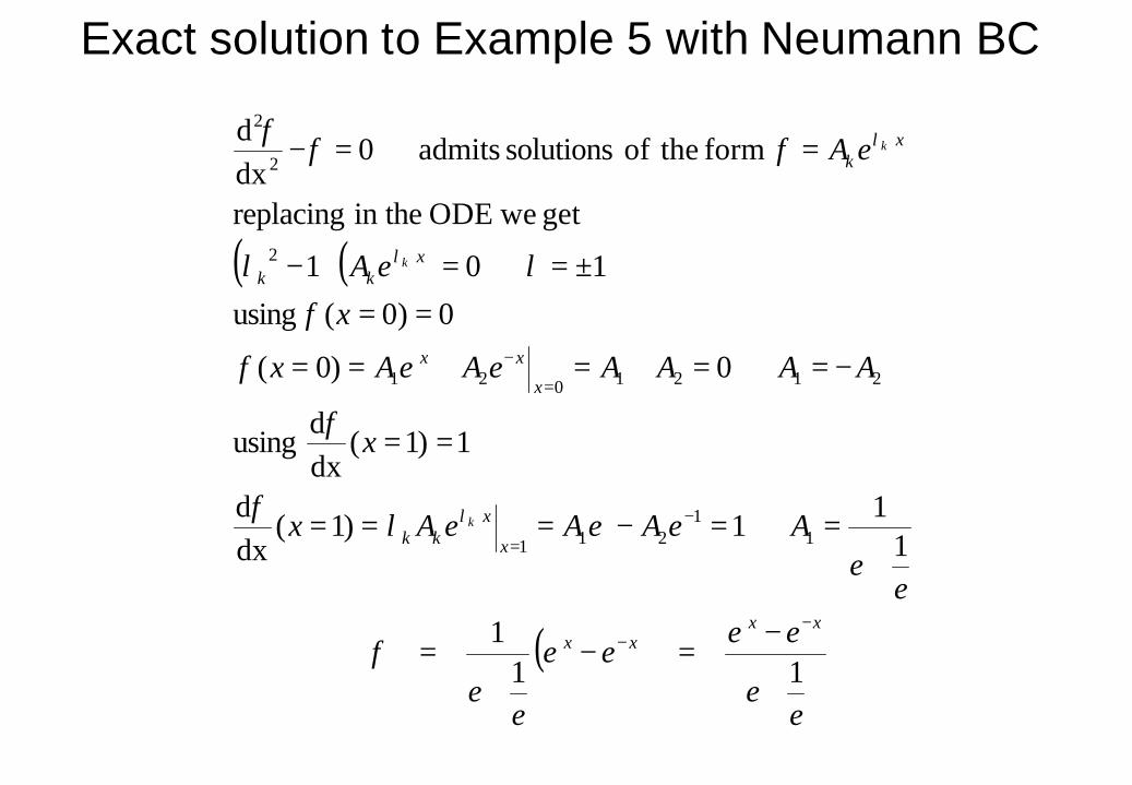
Exact solution to Example 5 with Neumann BC
( ) ( )
( )e
e
eeee
ee
ee
AeAeAeAx
x
AAAAeAeAx
x
eA
eA
xxxx
x
xkk
x
xx
xkk
xk
k
k
k
111
1
11)1(
dxd
1)1(dxd
using
0)0(
0)0( using
10 1
get weODE in the replacing
form theof solutions admits 0dxd
11
211
2121021
2
2
2
+
−=−
+=∴
+=⇒=−===
==
−=⇒=+=+==
==
±=⇒=−
==−
−−
−
=
=
−
φ
λφ
φ
φ
φ
λλ
φφφ
λ
λ
λ
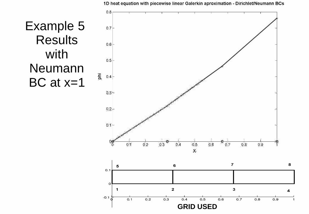
Example 5: Results
withNeumannBC at x=1
GRID USED

Example 5: Results
withNeumannBC at x=1
[phi , phi_th] = [ …0 0
2.192827911335199e-001 2.200407092120653e-0014.633853662097133e-001 4.647576055524206e-0017.599367659842332e-001 7.615941559557650e-001 ]
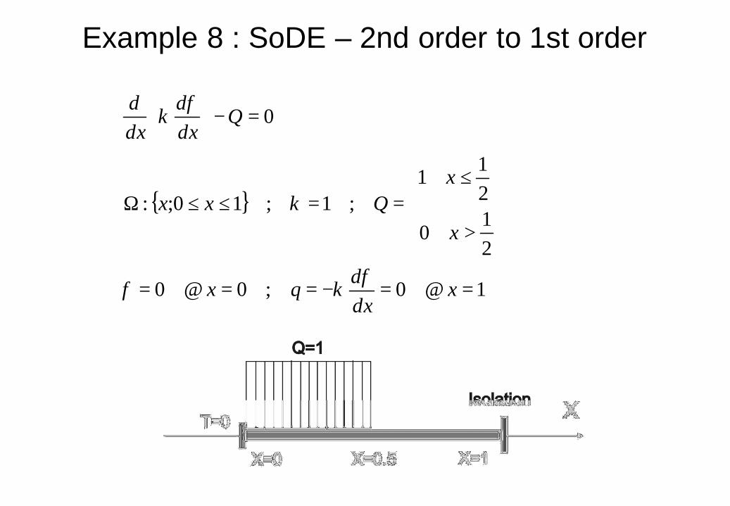
Example 8 : SoDE – 2nd order to 1st order
1@0;0@0
21
0
21
1;1;10;:
0
==−===
>
≤==≤≤Ω
=−
xdxd
qx
x
xQxx
Qdxd
dxd
φκφ
κ
φκ
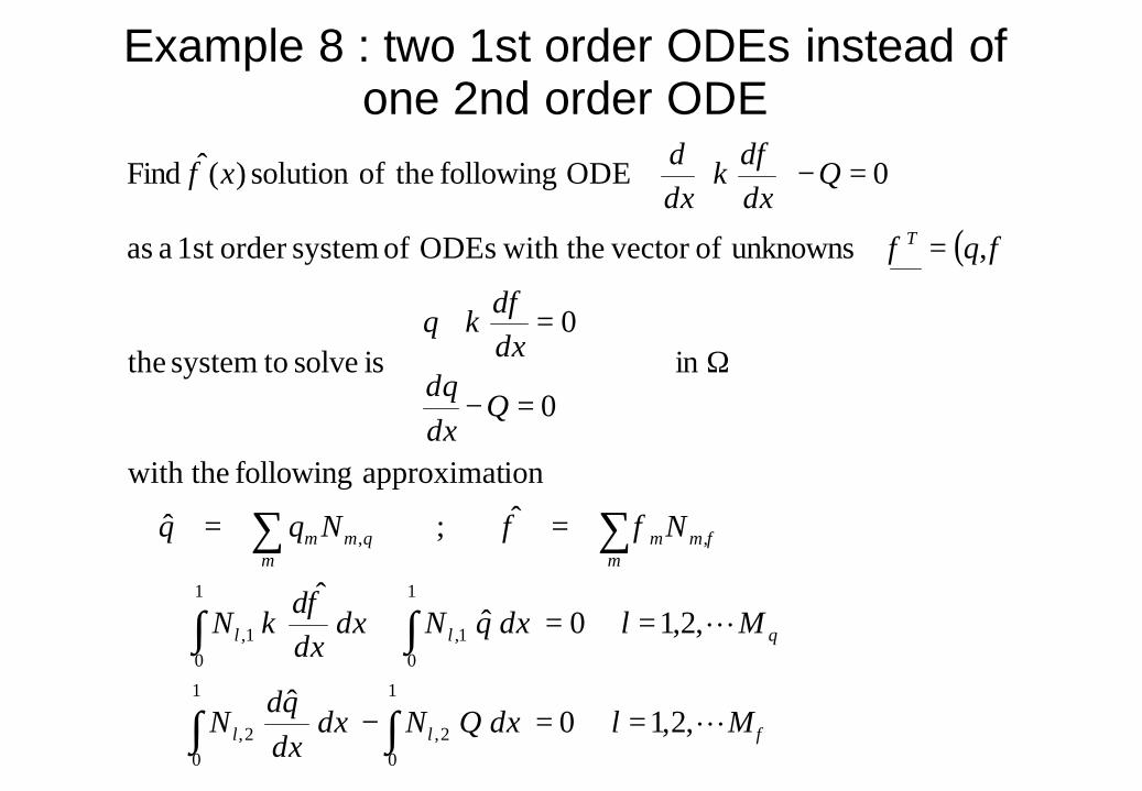
Example 8 : two 1st order ODEs instead ofone 2nd order ODE
( )
φ
φ
φκ
φφ
φκ
φφ
φκφ
MldxQNdxdxqd
N
MldxqNdxdxd
N
NNqq
Qdxdq
dxd
q
q
Qdxd
dxd
x
ll
qll
mmm
mqmm
T
L
L
,2,1 0ˆ
,2,1 0ˆˆ
ˆ;ˆ
ionapproximat following with the
in 0
0 is solve tosystem the
, unknowns of vector with theODEs of systemorder 1st a as
0 ODE following theofsolution )(ˆ Find
1
02,
1
02,
1
01,
1
01,
,,
==−
==+∴
==
Ω
=−
=+
=
=−
∫∫
∫∫
∑∑
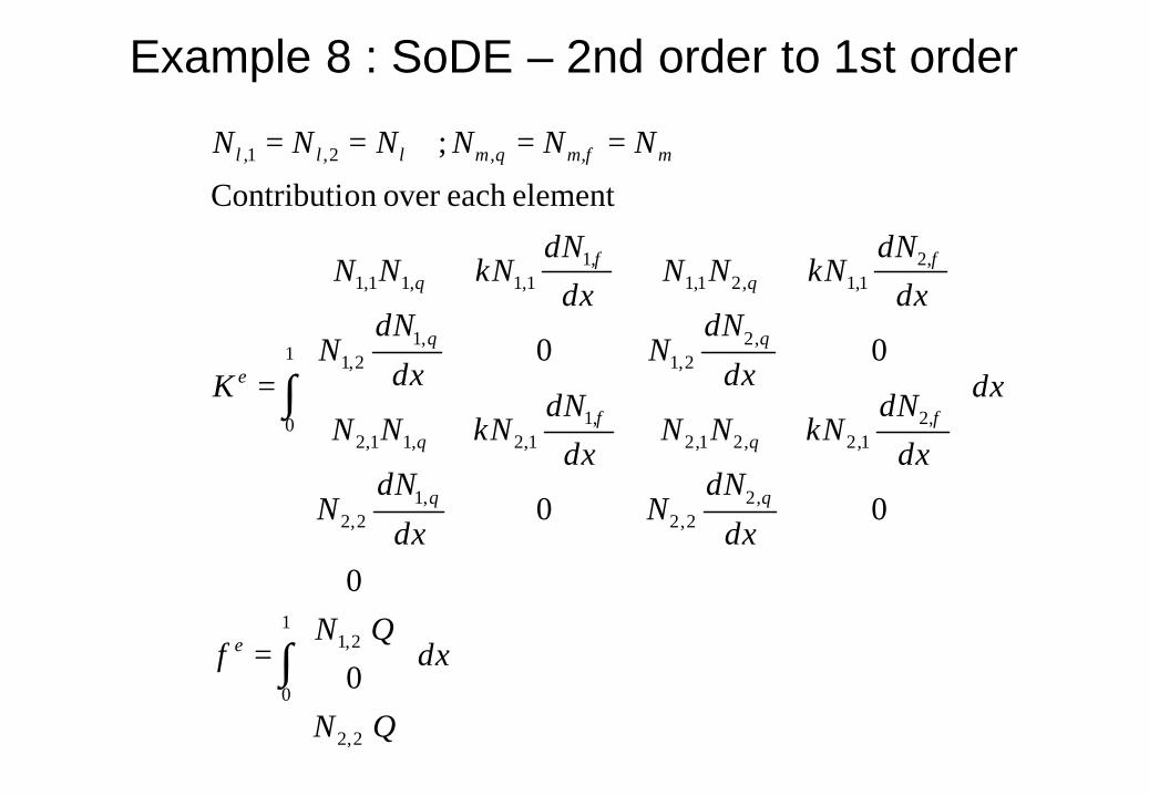
Example 8 : SoDE – 2nd order to 1st order
dx
QN
QNf
dx
dx
dNN
dx
dNN
dxdN
NNNdx
dNNNN
dx
dNN
dx
dNN
dxdN
NNNdx
dNNNN
K
NNNNNN
e
e
mmqmlll
∫
∫
=
=
====
1
0
2,2
2,1
1
0
,22,2
,12,2
,21,2,21,2
,11,2,11,2
,22,1
,12,1
,21,1,21,1
,11,1,11,1
,,2,1,
0
0
00
00
elementeach over on Contributi
;
φφ
φφ
φ
κκ
κκ
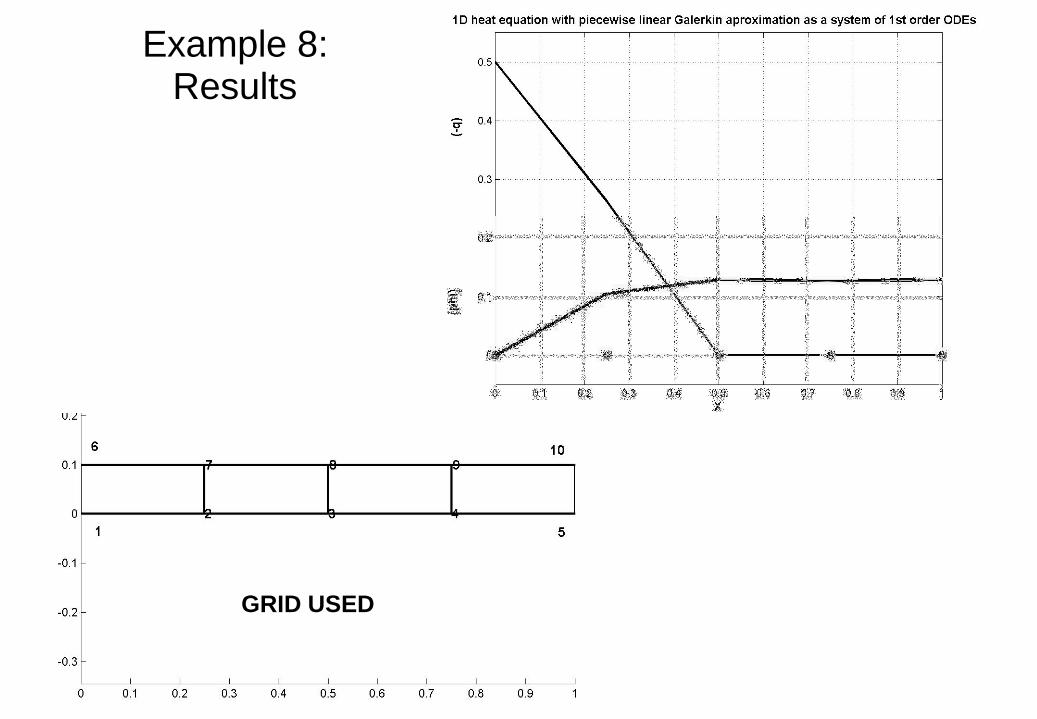
Example 8: Results
GRID USED
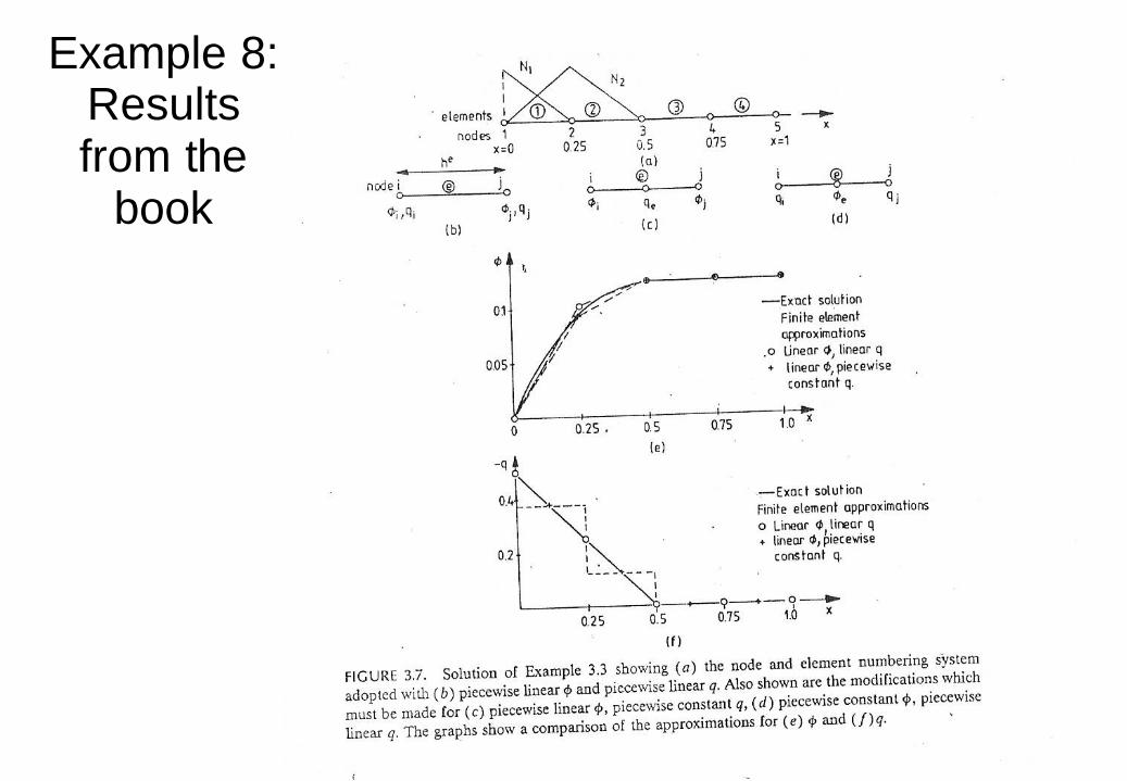
Example 8: Resultsfrom the
book
Weak form and mixed formulation
Some figure with weight and trialFunctions for different fields
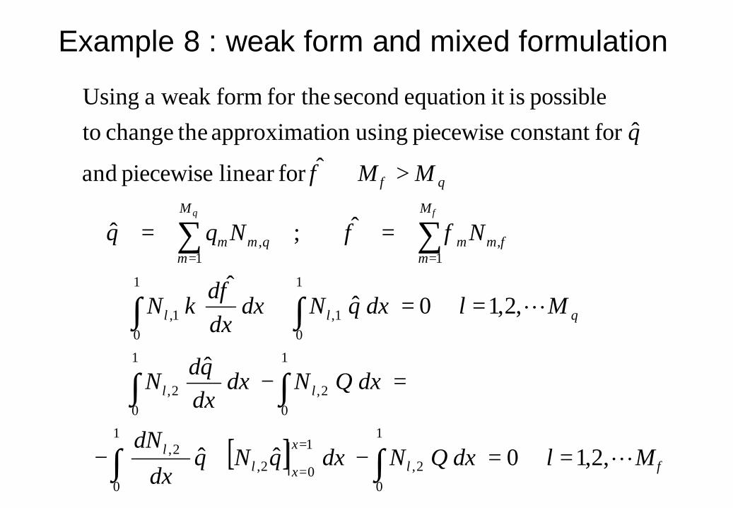
Example 8 : weak form and mixed formulation
[ ] φ
φ
φ
φκ
φφ
φφ
MldxQNdxqNqdx
dN
dxQNdxdxqd
N
MldxqNdxdxd
N
NNqq
MM
q
l
x
xll
ll
qll
M
mmm
M
mqmm
q
q
L
L
,2,1 0ˆˆ
ˆ
,2,1 0ˆˆ
ˆ;ˆ
ˆfor linear piecewise and
ˆfor constant piecewise usingion approximat thechange topossible isit equation second for the form weak a Using
1
02,
1
0
1
02,2,
1
02,
1
02,
1
01,
1
01,
1,
1,
==−+−
=−
==+∴
==
>⇒
∫∫
∫∫
∫∫
∑∑
=
=
==
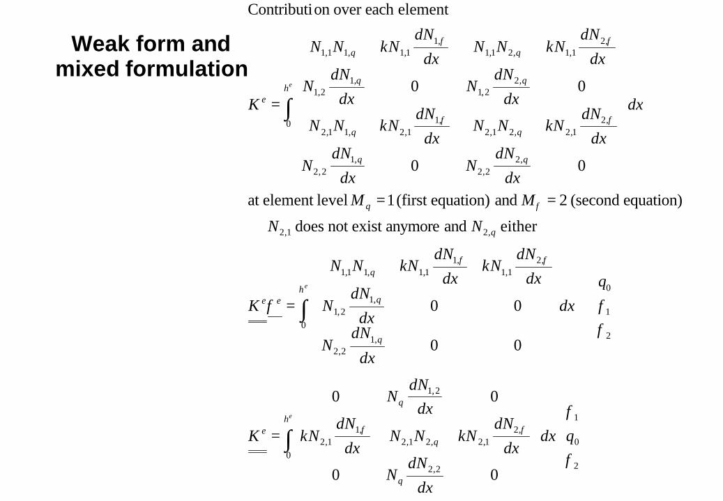
Weak form andmixed formulation
=
=
⇒
==
=
∫
∫
∫
2
0
1
02,2
,21,2,21,2
,11,2
2,1
2
1
0
0
,12,2
,12,1
,21,1
,11,1,11,1
,21,2
0
,22,2
,12,2
,21,2,21,2
,11,2,11,2
,22,1
,12,1
,21,1,21,1
,11,1,11,1
00
00
00
00
either and anymoreexist not does
equation) (second 2 and equation)(first 1 levelelement at
00
00
elementeach over on Contributi
φ
φκκ
φφ
κκ
φ
κκ
κκ
φφ
φφ
φ
φφ
φφ
qdx
dx
dNN
dx
dNNNN
dx
dNN
dxdN
N
K
q
dx
dx
dNN
dx
dNN
dx
dNN
dx
dNNNN
K
NN
MM
dx
dx
dNN
dx
dNN
dx
dNNNN
dx
dNNNN
dx
dNN
dx
dNN
dx
dNNNN
dx
dNNNN
K
e
e
e
h
q
q
q
e
h
q
q
q
ee
q
q
h
e
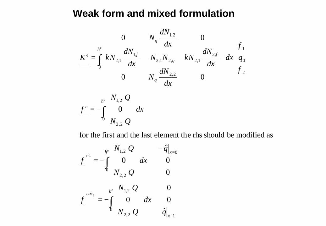
Weak form and mixed formulation
+
−=
−+
−=
−=
=
=
=
∫
∫
∫
∫
=
=
10
2,2
2,1
0
02,2
2,1
02,2
2,1
2
0
1
0
2,2
,21,2,21,2
,11,2
2,1
ˆ00
0
00
ˆ
0
as modified be should rhs eelement thlast theandfirst for the
0
00
00
1
x
h
xh
he
h
q
q
q
e
qdx
QN
QNf
qdx
QN
QNf
dxQN
QNf
qdx
dxdN
N
dx
dNNNN
dx
dNN
dxdN
N
K
eqMe
ee
e
e
φ
φκκ φφ
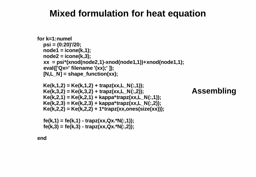
Mixed formulation for heat equation
for k=1:numelpsi = (0:20)'/20; node1 = icone(k,1);node2 = icone(k,3);xx = psi*(xnod(node2,1)-xnod(node1,1))+xnod(node1,1); eval(['Qx=' filename '(xx);' ]);[N,L_N] = shape_function(xx);
Ke(k,1,2) = Ke(k,1,2) + trapz(xx,L_N(:,1)); Ke(k,3,2) = Ke(k,3,2) + trapz(xx,L_N(:,2)); Ke(k,2,1) = Ke(k,2,1) + kappa*trapz(xx,L_N(:,1)); Ke(k,2,3) = Ke(k,2,3) + kappa*trapz(xx,L_N(:,2)); Ke(k,2,2) = Ke(k,2,2) + 1*trapz(xx,ones(size(xx)));
fe(k,1) = fe(k,1) - trapz(xx,Qx.*N(:,1)); fe(k,3) = fe(k,3) - trapz(xx,Qx.*N(:,2));
end
Assembling
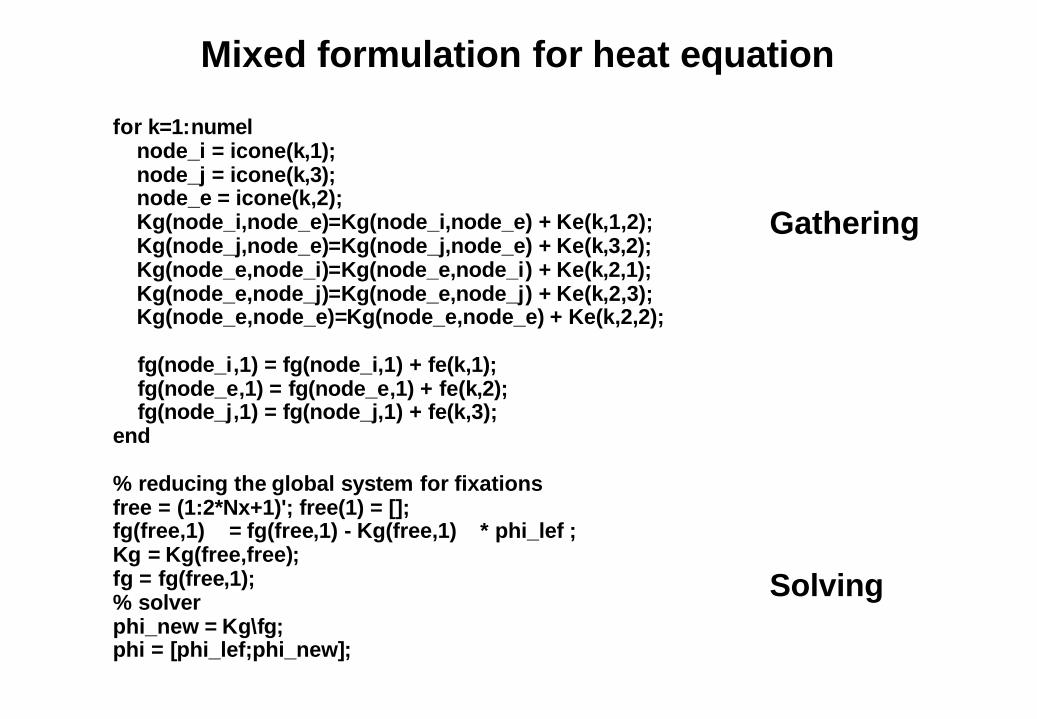
Mixed formulation for heat equation
Gathering
for k=1:numelnode_i = icone(k,1);node_j = icone(k,3);node_e = icone(k,2); Kg(node_i,node_e)=Kg(node_i,node_e) + Ke(k,1,2); Kg(node_j,node_e)=Kg(node_j,node_e) + Ke(k,3,2);Kg(node_e,node_i)=Kg(node_e,node_i) + Ke(k,2,1);Kg(node_e,node_j)=Kg(node_e,node_j) + Ke(k,2,3); Kg(node_e,node_e)=Kg(node_e,node_e) + Ke(k,2,2);
fg(node_i,1) = fg(node_i,1) + fe(k,1);fg(node_e,1) = fg(node_e,1) + fe(k,2);fg(node_j,1) = fg(node_j,1) + fe(k,3);
end
% reducing the global system for fixationsfree = (1:2*Nx+1)'; free(1) = [];fg(free,1) = fg(free,1) - Kg(free,1) * phi_lef ;Kg = Kg(free,free);fg = fg(free,1);% solverphi_new = Kg\fg;phi = [phi_lef;phi_new];
Solving
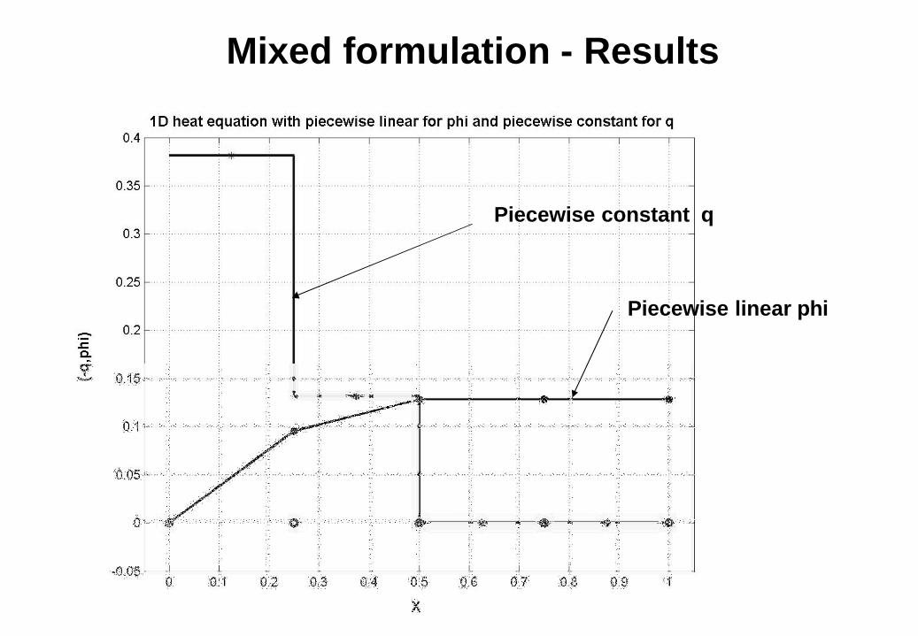
Mixed formulation - Results
Piecewise constant q
Piecewise linear phi
Generalization to 2D and 3D problems
• 1D problems are attractive to check numerical schemes (exactsolution availability)
• 1D problems have little practical (industrial) interests• 2D or 3D problems have analytical solution only for very simple
geometries and boundary conditions• In general only numerical methods may be used• In 2D and 3D the choice of the shape functions depends on the
equation to be solved and the type of element being used. • Triangular and quadrangular types are commonly used (not
necessarily restricted to these).• In 3D tetrahedra are widely used because of mesh generators
availability. • Hexahedra are less common but they are attractive for their
accuracy if the geometry allows for them.• Prismatic elements close to bodies where boundary layer are
expected may be included.• 2D & 3D the idea is to cover the whole domain with simple non-
overlapping elements
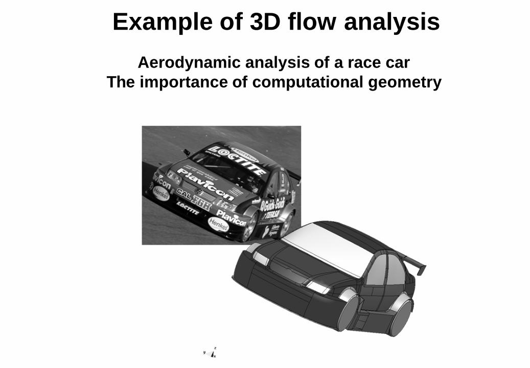
Example of 3D flow analysis
Aerodynamic analysis of a race carThe importance of computational geometry
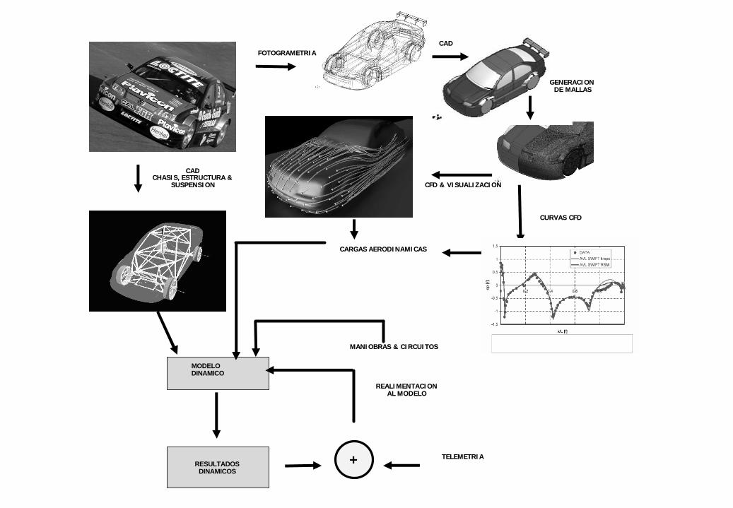
FOTOGRAMETRIAFOTOGRAMETRIACADCAD
GENERACION GENERACION DE MALLASDE MALLAS
CFDCFD & VISUALIZACION& VISUALIZACION
CARGAS AERODINAMICASCARGAS AERODINAMICAS
CADCADCHASIS, ESTRUCTURA & CHASIS, ESTRUCTURA &
SUSPENSIONSUSPENSION
MODELO DINAMICO
MANIOBRAS & CIRCUITOSMANIOBRAS & CIRCUITOS
CURVAS CFDCURVAS CFD
REALIMENTACIONREALIMENTACIONAL MODELOAL MODELO
TELEMETRIATELEMETRIARESULTADOS
DINAMICOS+
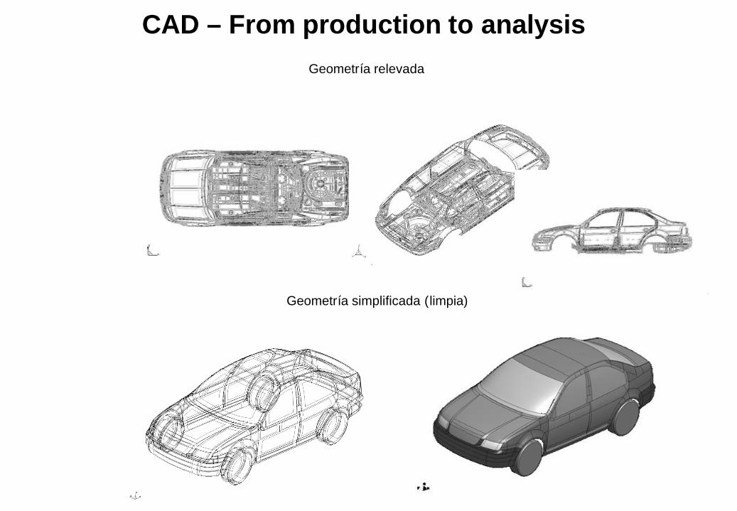
CAD – From production to analysisGeometría relevada
Geometría simplificada (limpia)
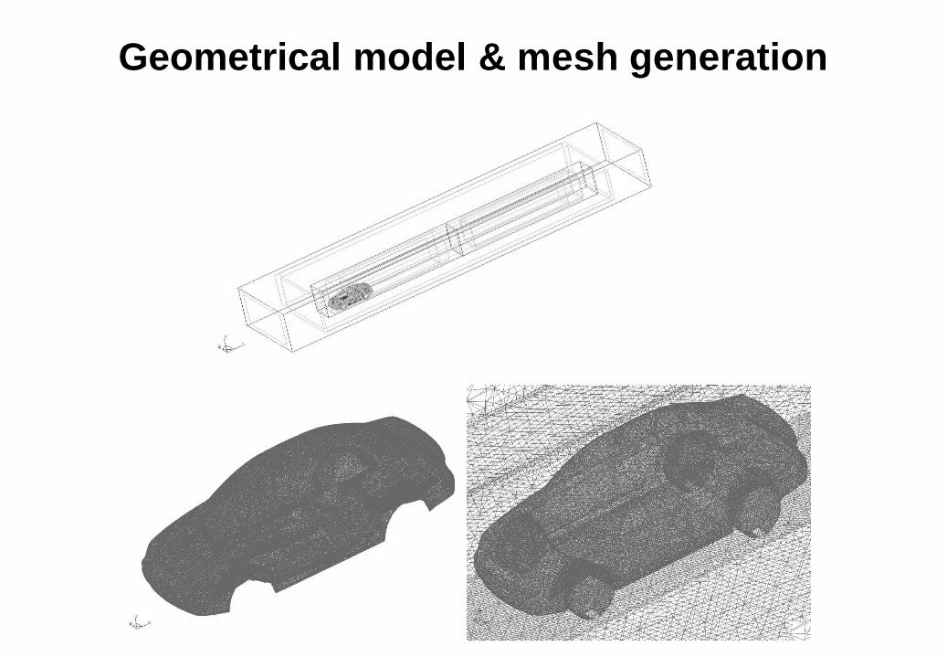
Geometrical model & mesh generation
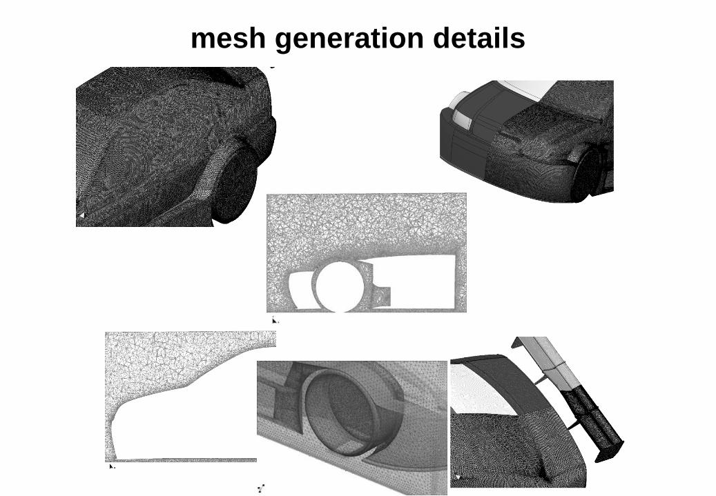
mesh generation details
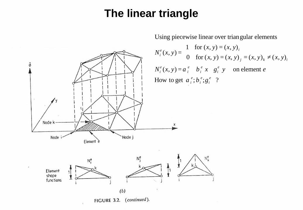
The linear triangle
? ;;get toHow
element on ),(
),(),(),(),(for 0
),(),(for 1),(
elementsgular over trianlinear piecewise Using
ei
ei
ei
ei
ei
ei
ei
ikj
iei
eyxyxN
yxyxyxyx
yxyxyxN
γβα
γβα ++=
≠==
==
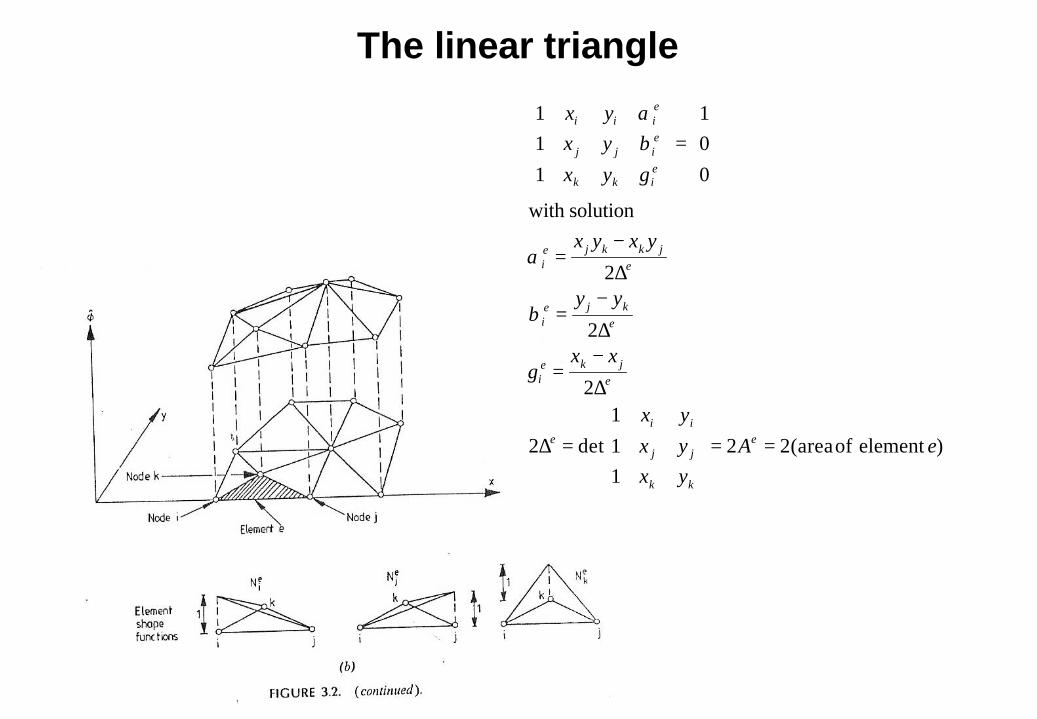
The linear triangle
)element of 2(area2111
det2
2
2
2
solutionwith
001
111
eAyxyxyx
xx
yy
yxyx
yxyxyx
e
kk
jj
iie
ejke
i
ekje
i
ejkkje
i
ei
ei
ei
kk
jj
ii
==
=∆
∆
−=
∆
−=
∆
−=
=
γ
β
α
γβα
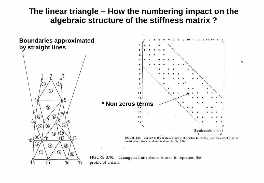
The linear triangle – How the numbering impact on thealgebraic structure of the stiffness matrix ?
Boundaries approximatedby straight lines
* Non zeros terms
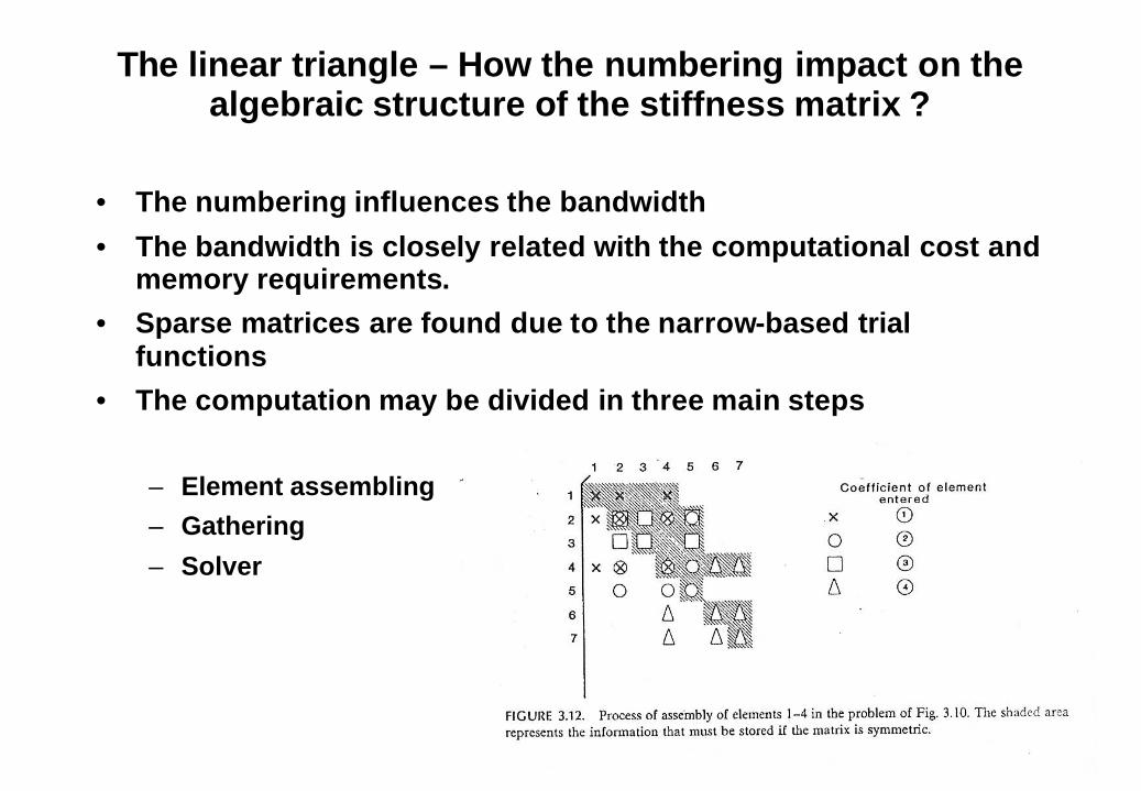
The linear triangle – How the numbering impact on thealgebraic structure of the stiffness matrix ?
• The numbering influences the bandwidth
• The bandwidth is closely related with the computational cost andmemory requirements.
• Sparse matrices are found due to the narrow-based trialfunctions
• The computation may be divided in three main steps
– Element assembling– Gathering
– Solver
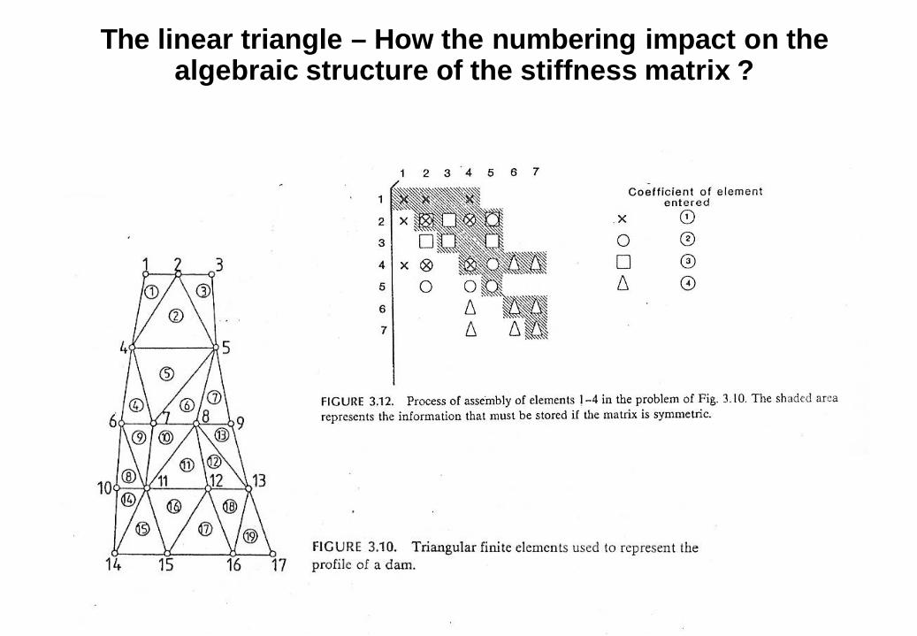
The linear triangle – How the numbering impact on thealgebraic structure of the stiffness matrix ?
* Non zeros terms
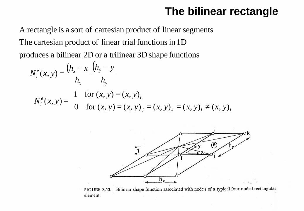
The bilinear rectangle
( ) ( )
≠====
=∴
−−=
),(),(),(),(),(for 0
),(),(for 1),(
),(
functions shape 3D trilinearaor 2Dbilinear a produces
1Din functions allinear tri ofproduct cartesian Thesegmentslinear ofproduct cartesian ofsort a is rectangleA
ilkj
iei
y
y
x
xei
yxyxyxyxyx
yxyxyxN
h
yh
hxh
yxN
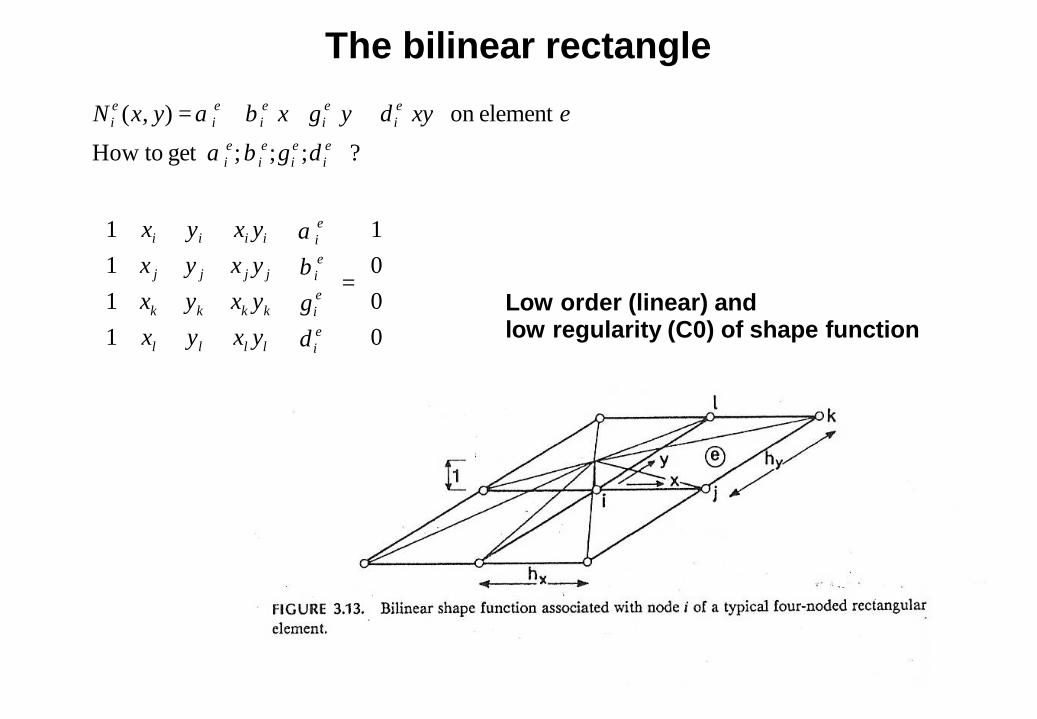
The bilinear rectangle
=
+++=
0001
1111
? ;;;get toHow
element on ),(
ei
ei
ei
ei
llll
kkkk
jjjj
iiii
ei
ei
ei
ei
ei
ei
ei
ei
ei
yxyxyxyxyxyxyxyx
exyyxyxN
δγβα
δγβα
δγβα
Low order (linear) andlow regularity (C0) of shape function
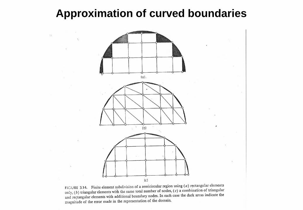
Approximation of curved boundaries
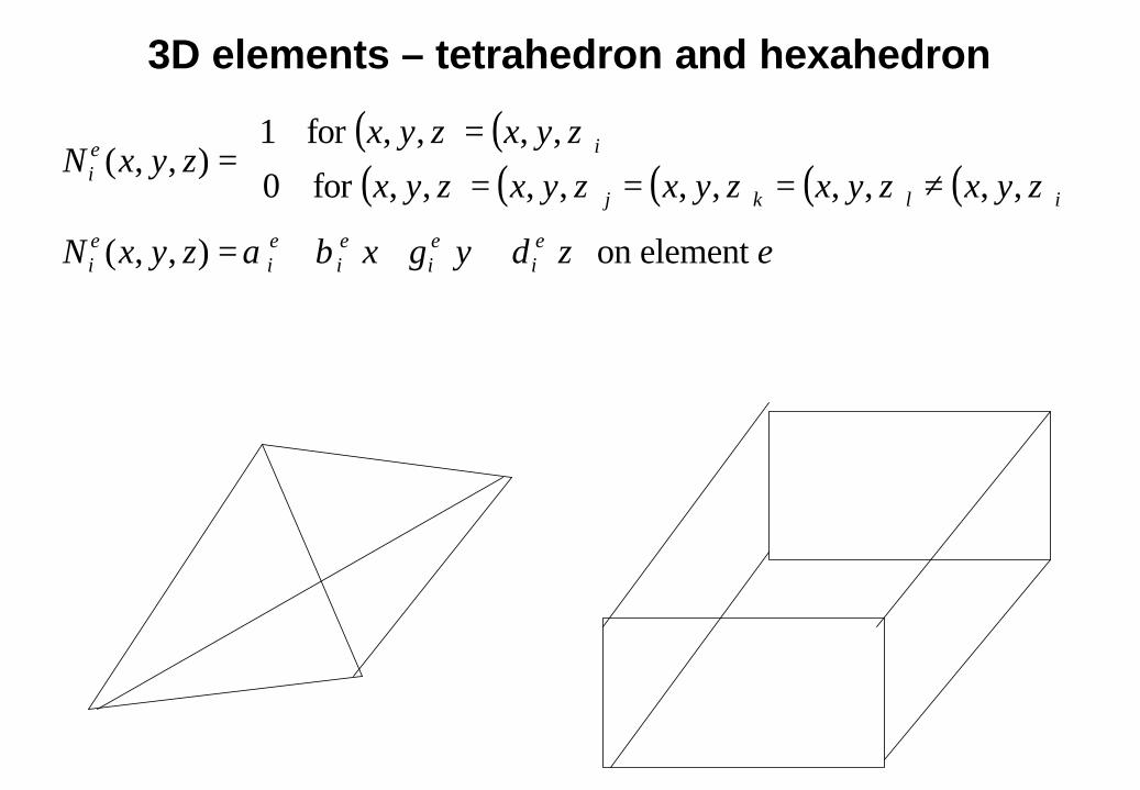
3D elements – tetrahedron and hexahedron
( ) ( )( ) ( ) ( ) ( ) ( )
ezyxzyxN
zyxzyxzyxzyxzyx
zyxzyxzyxN
ei
ei
ei
ei
ei
ilkj
iei
element on ),,(
,,,,,,,,,,for 0
,,,,for 1),,(
δγβα +++=
≠===
==