Embed Size (px)
Citation preview

Copyright © 2008 Pearson Education, Inc. Slide 2 - 28
Chapter 8
Confidence Intervals for
One Population Mean
Copyright © 2008 Pearson Education, Inc. Slide 3 - 28
Definition 8.1
Copyright © 2008 Pearson Education, Inc. Slide 4 - 28
Definition 8.2
Copyright © 2008 Pearson Education, Inc. Slide 5 - 28
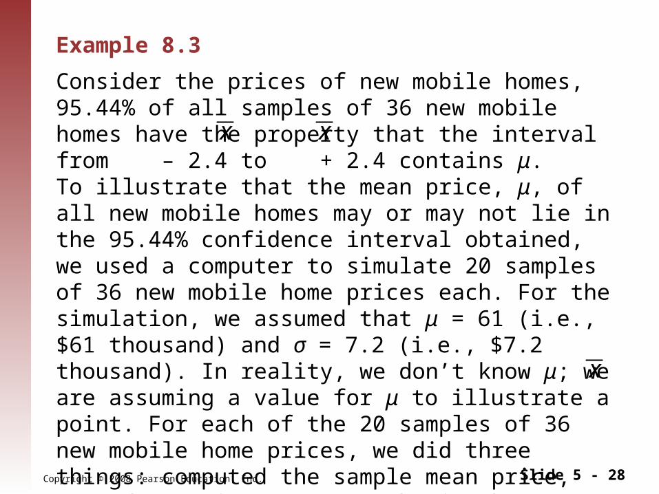
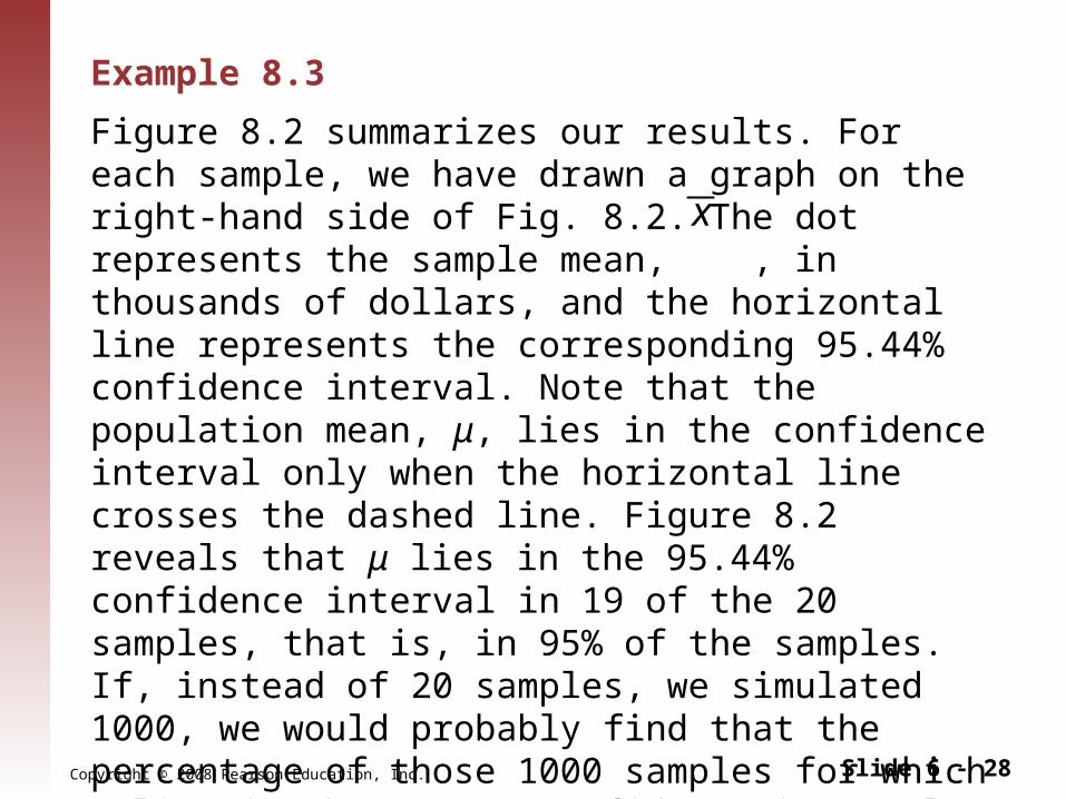
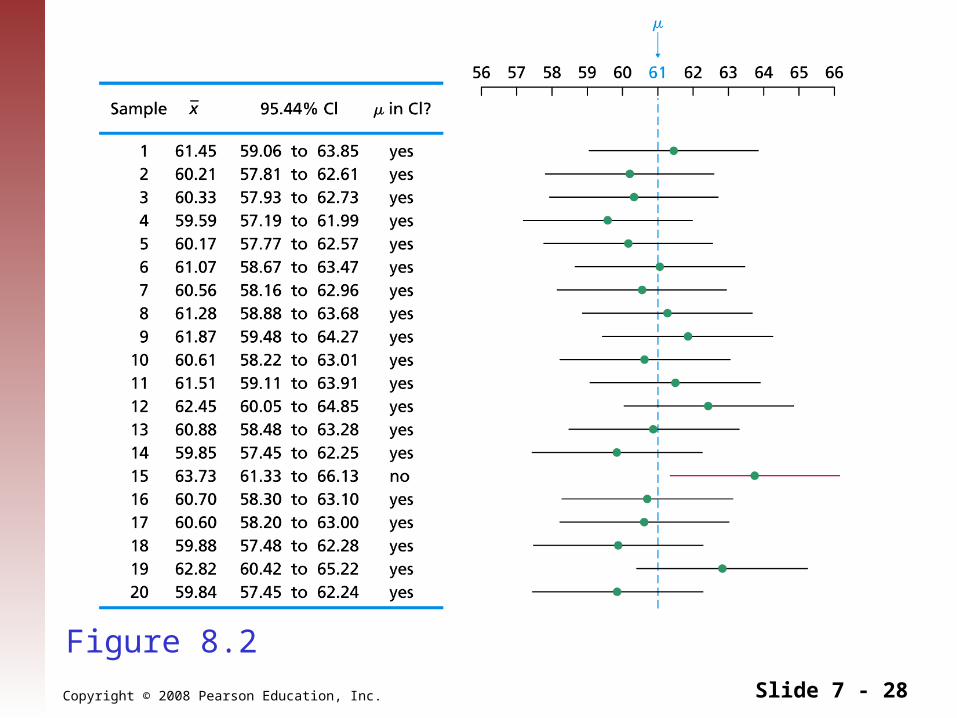
Example 8.3
Consider the prices of new mobile homes, 95.44% of all samples of 36 new mobile homes have the property that the interval from – 2.4 to + 2.4 contains μ.To illustrate that the mean price, μ, of all new mobile homes may or may not lie in the 95.44% confidence interval obtained, we used a computer to simulate 20 samples of 36 new mobile home prices each. For the simulation, we assumed that μ = 61 (i.e., $61 thousand) and σ = 7.2 (i.e., $7.2 thousand). In reality, we don’t know μ; we are assuming a value for μ to illustrate a point. For each of the 20 samples of 36 new mobile home prices, we did three things: computed the sample mean price, ; used Equation (8.1) to obtain the 95.44% confidence interval; and noted whether the population mean, μ = 61, actually lies in the confidence interval.
x
x x
Copyright © 2008 Pearson Education, Inc. Slide 6 - 28
Example 8.3
Figure 8.2 summarizes our results. For each sample, we have drawn a graph on the right-hand side of Fig. 8.2. The dot represents the sample mean, , in thousands of dollars, and the horizontal line represents the corresponding 95.44% confidence interval. Note that the population mean, μ, lies in the confidence interval only when the horizontal line crosses the dashed line. Figure 8.2 reveals that μ lies in the 95.44% confidence interval in 19 of the 20 samples, that is, in 95% of the samples. If, instead of 20 samples, we simulated 1000, we would probably find that the percentage of those 1000 samples for which μ lies in the 95.44% confidence interval would be even closer to 95.44%. Hence we can be 95.44% confident that any computed 95.44% confidence interval will contain μ.
x
Copyright © 2008 Pearson Education, Inc. Slide 7 - 28
Figure 8.2
Copyright © 2008 Pearson Education, Inc. Slide 8 - 28
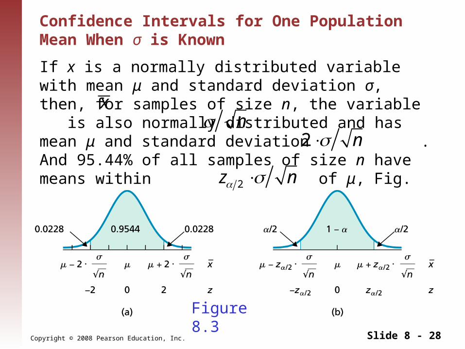
If x is a normally distributed variable with mean μ and standard deviation σ, then, for samples of size n, the variable is also normally distributed and has mean μ and standard deviation . And 95.44% of all samples of size n have means within of μ, Fig. 8.3(a). We can say that 100(1 − α)% of all samples of size n have means within of μ, Fig. 8.3(b).
x
Figure 8.3
Confidence Intervals for One Population Mean When σ is Known
n2 n
z 2 n
Copyright © 2008 Pearson Education, Inc. Slide 9 - 28
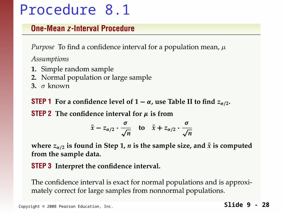
Procedure 8.1
Copyright © 2008 Pearson Education, Inc. Slide 10 - 28
Key Fact 8.1
Copyright © 2008 Pearson Education, Inc. Slide 11 - 28
Key Fact 8.2
Copyright © 2008 Pearson Education, Inc. Slide 12 - 28
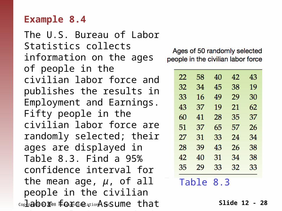
Example 8.4
The U.S. Bureau of Labor Statistics collects information on the ages of people in the civilian labor force and publishes the results in Employment and Earnings. Fifty people in the civilian labor force are randomly selected; their ages are displayed in Table 8.3. Find a 95% confidence interval for the mean age, μ, of all people in the civilian labor force. Assume that the population standard deviation of the ages is 12.1 years.
Table 8.3
Copyright © 2008 Pearson Education, Inc. Slide 13 - 28
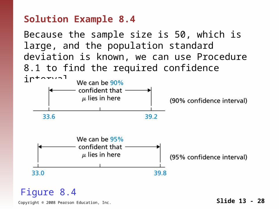
Solution Example 8.4
Because the sample size is 50, which is large, and the population standard deviation is known, we can use Procedure 8.1 to find the required confidence interval.
Figure 8.4
Copyright © 2008 Pearson Education, Inc. Slide 14 - 28
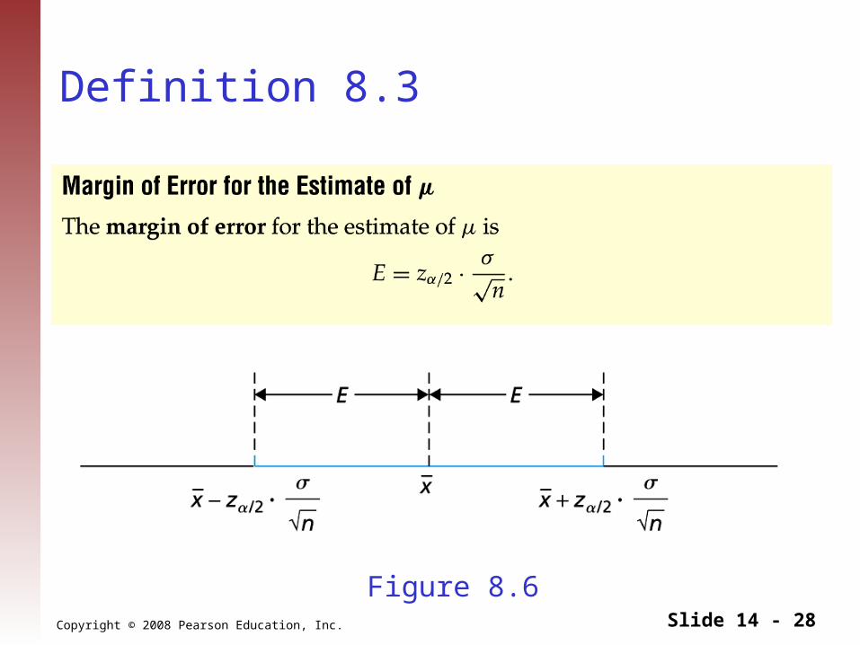
Definition 8.3
Figure 8.6
Copyright © 2008 Pearson Education, Inc. Slide 15 - 28
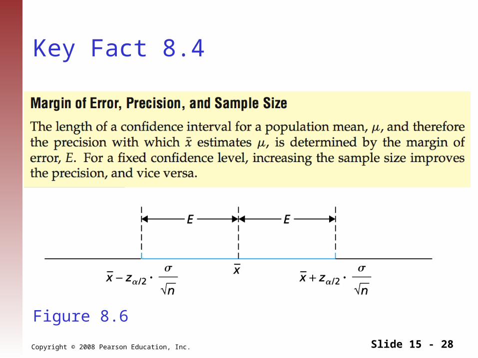
Key Fact 8.4
Figure 8.6

Copyright © 2008 Pearson Education, Inc. Slide 16 - 28
Formula 8.1
Copyright © 2008 Pearson Education, Inc. Slide 17 - 28
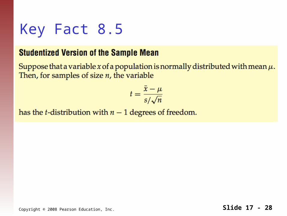
Key Fact 8.5
Copyright © 2008 Pearson Education, Inc. Slide 18 - 28
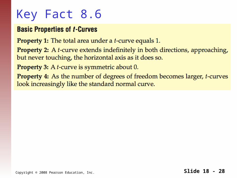
Key Fact 8.6
Copyright © 2008 Pearson Education, Inc. Slide 19 - 28
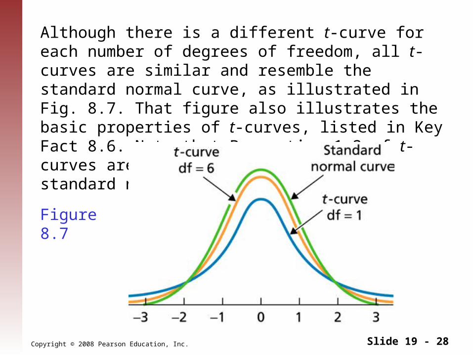
Although there is a different t-curve for each number of degrees of freedom, all t-curves are similar and resemble the standard normal curve, as illustrated in Fig. 8.7. That figure also illustrates the basic properties of t-curves, listed in Key Fact 8.6. Note that Properties 1–3 of t-curves are identical to those of the standard normal curve.
Figure 8.7
Copyright © 2008 Pearson Education, Inc. Slide 20 - 28
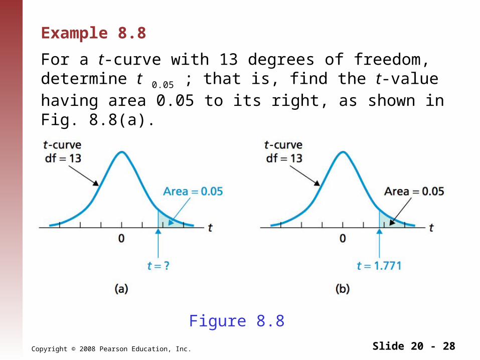
Example 8.8
For a t-curve with 13 degrees of freedom, determine t 0.05 ; that is, find the t-value having area 0.05 to its right, as shown in Fig. 8.8(a).
Figure 8.8
Copyright © 2008 Pearson Education, Inc. Slide 21 - 28
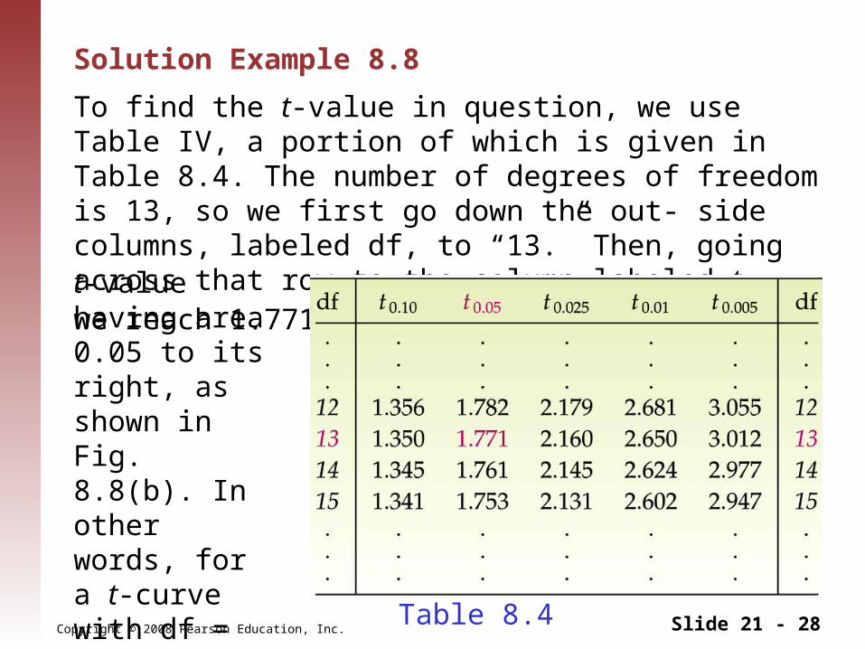
Solution Example 8.8
To find the t-value in question, we use Table IV, a portion of which is given in Table 8.4. The number of degrees of freedom is 13, so we first go down the out- side columns, labeled df, to “13.” Then, going across that row to the column labeled t0.05 , we reach 1.771. This number is the
Table 8.4
t-value having area 0.05 to its right, as shown in Fig. 8.8(b). In other words, for a t-curve with df = 13,t0.05 = 1.771.
Copyright © 2008 Pearson Education, Inc. Slide 22 - 28
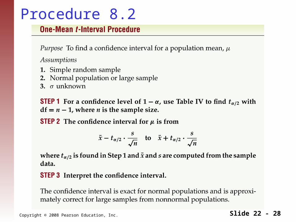
Procedure 8.2
Copyright © 2008 Pearson Education, Inc. Slide 23 - 28
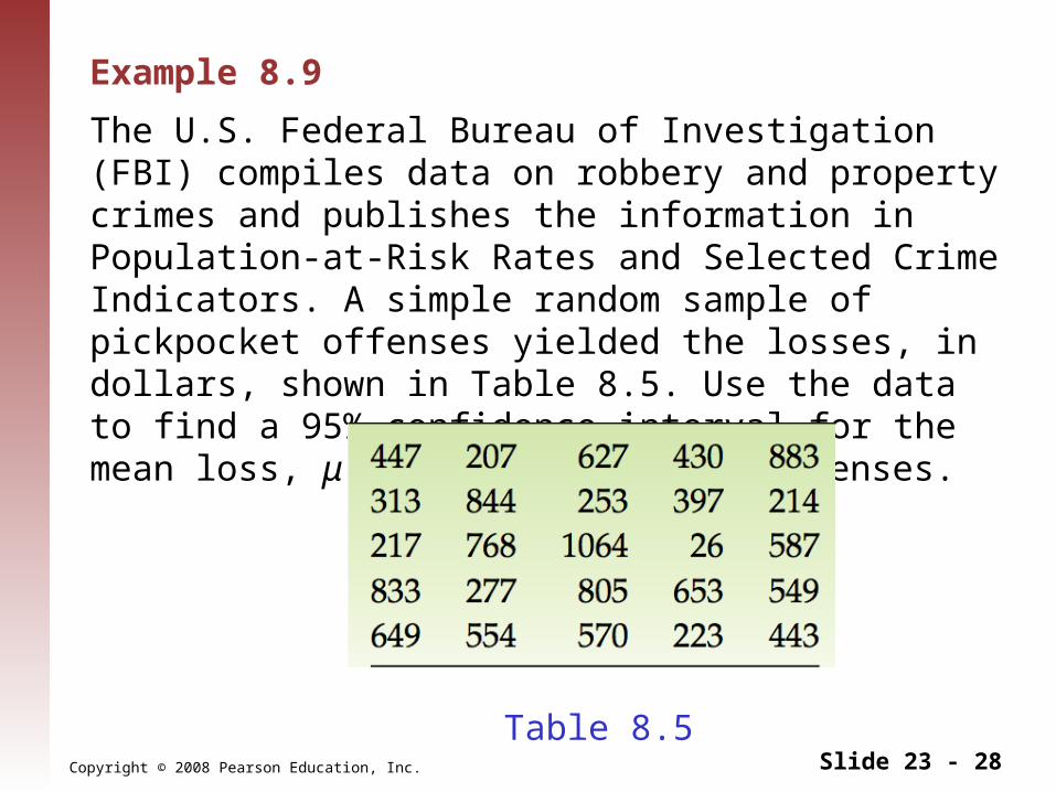
Example 8.9
The U.S. Federal Bureau of Investigation (FBI) compiles data on robbery and property crimes and publishes the information in Population-at-Risk Rates and Selected Crime Indicators. A simple random sample of pickpocket offenses yielded the losses, in dollars, shown in Table 8.5. Use the data to find a 95% confidence interval for the mean loss, μ, of all pickpocket offenses.
Table 8.5
Copyright © 2008 Pearson Education, Inc. Slide 24 - 28
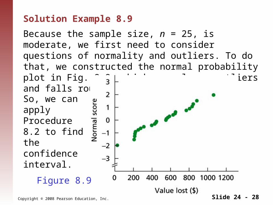
Solution Example 8.9
Because the sample size, n = 25, is moderate, we first need to consider questions of normality and outliers. To do that, we constructed the normal probability plot in Fig. 8.9, which reveals no outliers and falls roughly in a straight line.
So, we can apply Procedure 8.2 to find the confidence interval.
Figure 8.9
Copyright © 2008 Pearson Education, Inc. Slide 25 - 28
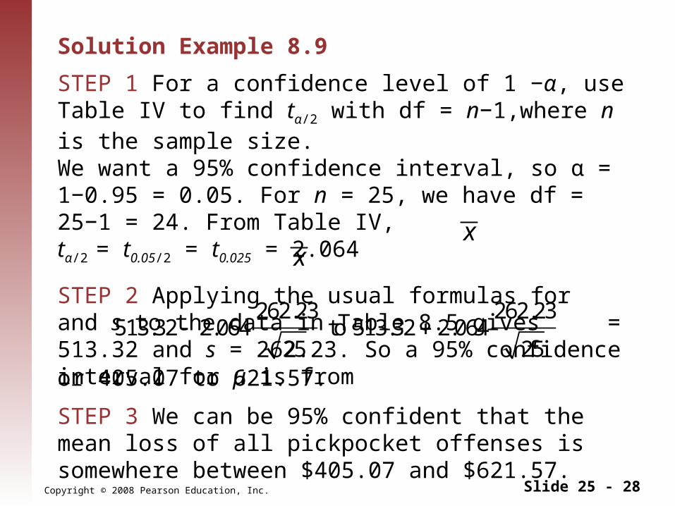
Solution Example 8.9
STEP 1 For a confidence level of 1 −α, use Table IV to find tα/2 with df = n−1,where n is the sample size.We want a 95% confidence interval, so α = 1−0.95 = 0.05. For n = 25, we have df = 25−1 = 24. From Table IV, tα/2 = t0.05/2 = t0.025 = 2.064
STEP 2 Applying the usual formulas for and s to the data in Table 8.5 gives = 513.32 and s = 262.23. So a 95% confidence interval for μ is from
xx
or 405.07 to 621.57.
STEP 3 We can be 95% confident that the mean loss of all pickpocket offenses is somewhere between $405.07 and $621.57.
513.32 2.064262.23
25 to 513.32 2.064
262.23
25
Copyright © 2008 Pearson Education, Inc. Slide 26 - 28
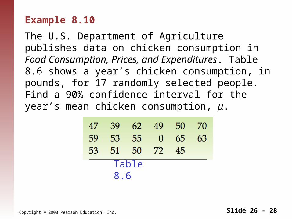
Example 8.10
The U.S. Department of Agriculture publishes data on chicken consumption in Food Consumption, Prices, and Expenditures. Table 8.6 shows a year’s chicken consumption, in pounds, for 17 randomly selected people. Find a 90% confidence interval for the year’s mean chicken consumption, μ.
Table 8.6
Copyright © 2008 Pearson Education, Inc. Slide 27 - 28
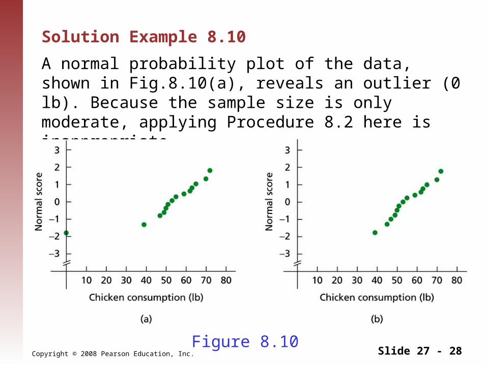
Solution Example 8.10
A normal probability plot of the data, shown in Fig.8.10(a), reveals an outlier (0 lb). Because the sample size is only moderate, applying Procedure 8.2 here is inappropriate.
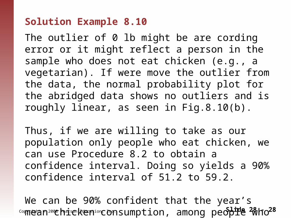
Figure 8.10
Copyright © 2008 Pearson Education, Inc. Slide 28 - 28
Solution Example 8.10
The outlier of 0 lb might be are cording error or it might reflect a person in the sample who does not eat chicken (e.g., a vegetarian). If were move the outlier from the data, the normal probability plot for the abridged data shows no outliers and is roughly linear, as seen in Fig.8.10(b).
Thus, if we are willing to take as our population only people who eat chicken, we can use Procedure 8.2 to obtain a confidence interval. Doing so yields a 90% confidence interval of 51.2 to 59.2.
We can be 90% confident that the year’s mean chicken consumption, among people who eat chicken, is somewhere between 51.2 lb and 59.2 lb.