Slide 1 - Introduction to Statistics Tutorial: Probability and Probability Distributions Part 1

Slide notes Introduction to Statistics Tutorial: Probability and Probability Distributions. This tutorial is the third in a series of several tutorials that introduce probability and statistics. Here we will concentrate on elementary probability and probability distributions.

Slide 2 - Outline

Slide notes Throughout this tutorial, we will present definitions and notation for probability. We will introduce concepts such as complement, compound event, union, intersection, probability rules and discrete probability distributions.

Slide 3 - Probability - 1

Slide notes Probability is very important to statistics: it is the tool that gives the statistician the ability to use sample information to make inference about or to describe the population from which the sample was drawn.

Slide 4 - Probability: definitions

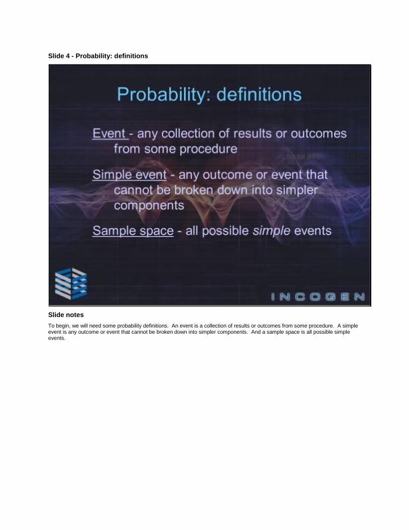
Slide notes To begin, we will need some probability definitions. An event is a collection of results or outcomes from some procedure. A simple event is any outcome or event that cannot be broken down into simpler components. And a sample space is all possible simple events.

Slide 5 - Probability: Notation

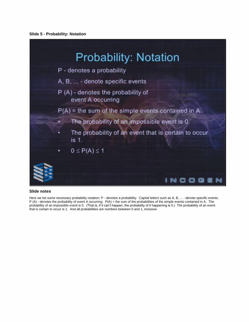
Slide notes Here we list some necessary probability notation: P - denotes a probability. Capital letters such as A, B, ... - denote specific events. P (A) - denotes the probability of event A occurring. P(A) = the sum of the probabilities of the simple events contained in A. The probability of an impossible event is 0. (That is, if it can’t happen, the probability of it happening is 0.) The probability of an event that is certain to occur is 1. And all probabilities are numbers between 0 and 1, inclusive.

Slide 6 - Simple Probability Example

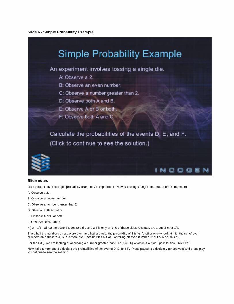
Slide notes Let’s take a look at a simple probability example: An experiment involves tossing a single die. Let's define some events. A: Observe a 2. B: Observe an even number. C: Observe a number greater than 2. D: Observe both A and B. E: Observe A or B or both. F: Observe both A and C. P(A) = 1/6. Since there are 6 sides to a die and a 2 is only on one of those sides, chances are 1 out of 6, or 1/6. Since half the numbers on a die are even and half are odd, the probability of B is ½. Another way to look at it is, the set of even numbers on a die is 2, 4, 6. So there are 3 possibilities out of 6 of rolling an even number. 3 out of 6 or 3/6 = ½. For the P(C), we are looking at observing a number greater than 2 or {3,4,5,6} which is 4 out of 6 possibilities. 4/6 = 2/3. Now, take a moment to calculate the probabilities of the events D, E, and F. Press pause to calculate your answers and press play to continue to see the solution.

Slide 7 - Probability Example Continued - 1

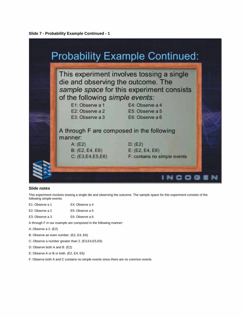
Slide notes This experiment involves tossing a single die and observing the outcome. The sample space for this experiment consists of the following simple events: E1: Observe a 1 E4: Observe a 4 E2: Observe a 2 E5: Observe a 5 E3: Observe a 3 E6: Observe a 6 A through F in our example are composed in the following manner: A: Observe a 2. (E2) B: Observe an even number. (E2, E4, E6) C: Observe a number greater than 2. (E3,E4,E5,E6) D: Observe both A and B. (E2) E: Observe A or B or both. (E2, E4, E6) F: Observe both A and C contains no simple events since there are no common events

Slide 8 - Probability Example Continued:

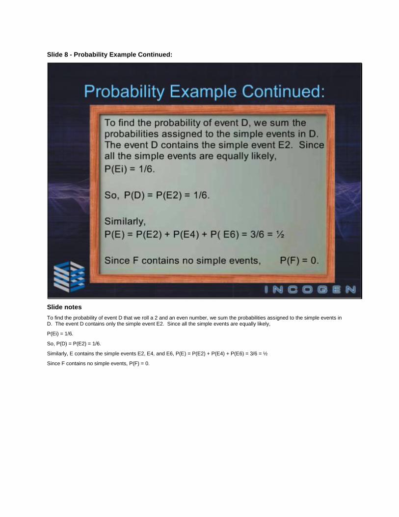
Slide notes To find the probability of event D that we roll a 2 and an even number, we sum the probabilities assigned to the simple events in D. The event D contains only the simple event E2. Since all the simple events are equally likely, P(Ei) = 1/6. So, P(D) = P(E2) = 1/6. Similarly, E contains the simple events E2, E4, and E6, P(E) = P(E2) + P(E4) + P(E6) = 3/6 = ½ Since F contains no simple events, P(F) = 0.

Slide 9 - Probability

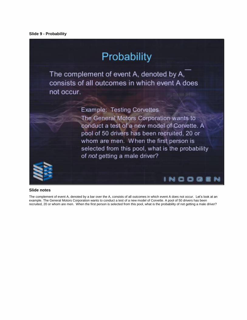
Slide notes The complement of event A, denoted by a bar over the A, consists of all outcomes in which event A does not occur. Let’s look at an example. The General Motors Corporation wants to conduct a test of a new model of Corvette. A pool of 50 drivers has been recruited, 20 or whom are men. When the first person is selected from this pool, what is the probability of not getting a male driver?

Slide 10 - Probability: Solution

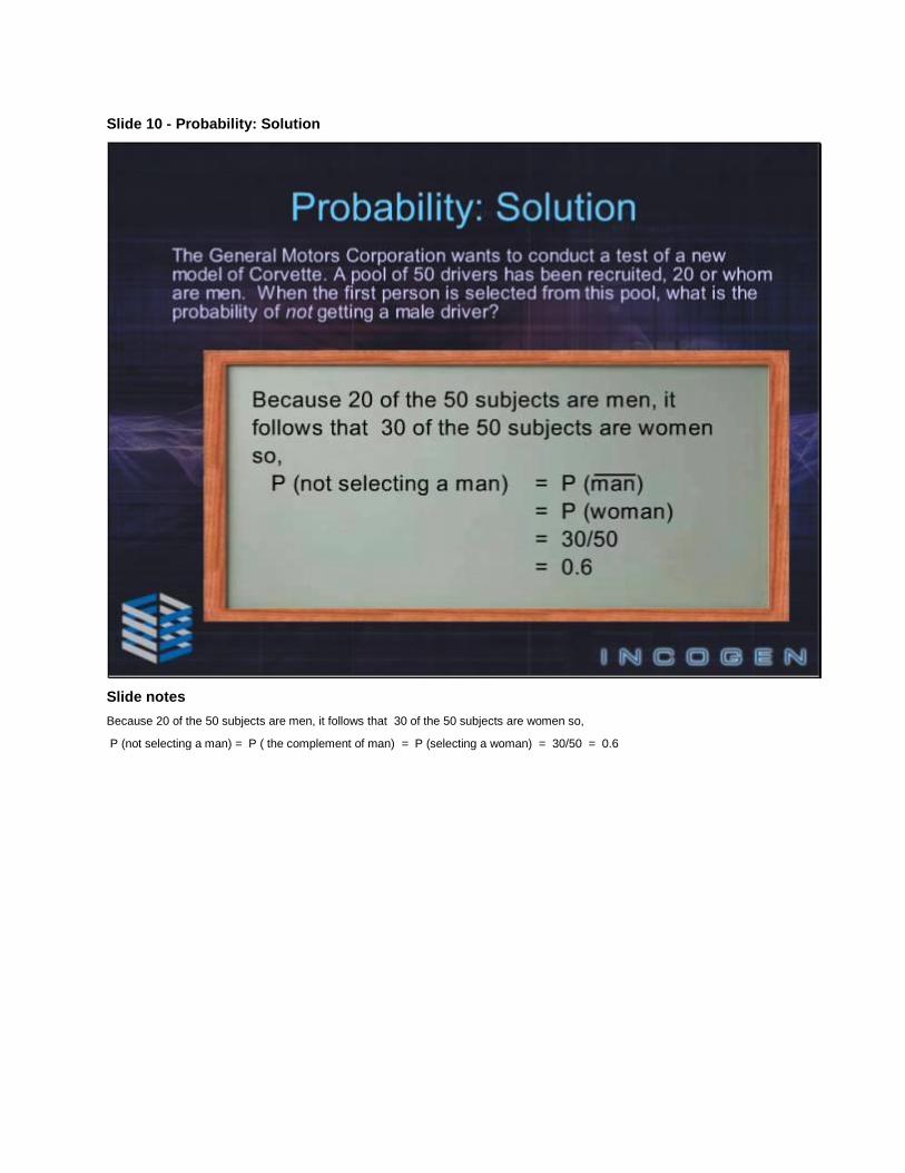
Slide notes Because 20 of the 50 subjects are men, it follows that 30 of the 50 subjects are women so,

P (not selecting a man) = P ( the complement of man) = P (selecting a woman) = 30/50 = 0.6

Slide 11 - Probability: Event Composition -1

Slide notes A compound Event is any event that is formed by combining 2 or more simple events. They can be formed by finding the union of 2 or more events, finding the intersection of 2 or more event, or by finding a combination of the 2. But what are unions and intersections of events?

Slide 12 - Probability: Event Composition -2

Slide notes The union of 2 events A and B is the event that A or B or both occur. The notation for the union of A and B is a“U” symbol between the A and B. The probability of the union of A and B is P(A or B); that is, it is equal to the P (event A occurs or event B occurs or both A and B occur).

Slide 13 - Probability: Event Composition -3

Slide notes In general, when finding the probability that event A occurs or event B occurs, find the total number of ways A can occur and the number of ways B can occur, but find the total in such a way that no outcome is counted more than once. So, to find P(AUB), find the sum of the number of ways event A can occur and the number of ways event B can occur, adding in such a way that every outcome is counted only once. The probability is equal to that sum, divided by the total number of outcomes.

Slide 14 - Probability: Event Composition -4

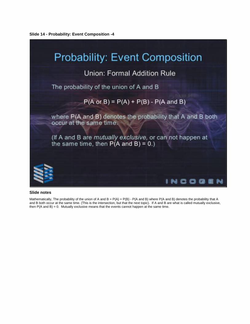
Slide notes Mathematically, The probability of the union of A and B = P(A) + P(B) - P(A and B) where P(A and B) denotes the probability that A and B both occur at the same time. (This is the intersection, but that the next topic). If A and B are what is called mutually exclusive, then P(A and B) = 0. Mutually exclusive means that the events cannot happen at the same time.

Slide 15 - Probability: Event Composition - 4

Slide notes Here is a Venn Diagram of the Union of A and B. Events A and B are represented by circles. They overlap (or intersect) if the two events contain the same simple events. If the two circles do not overlap, then the events are mutually exclusive.

Slide 16 - Probability: Event Composition - 5

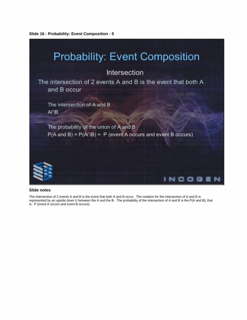
Slide notes The intersection of 2 events A and B is the event that both A and B occur. The notation for the intersection of A and B is represented by an upside down U between the A and the B. The probability of the intersection of A and B is the P(A and B); that is, P (event A occurs and event B occurs).

Slide 17 - Probability: Event Composition - 6

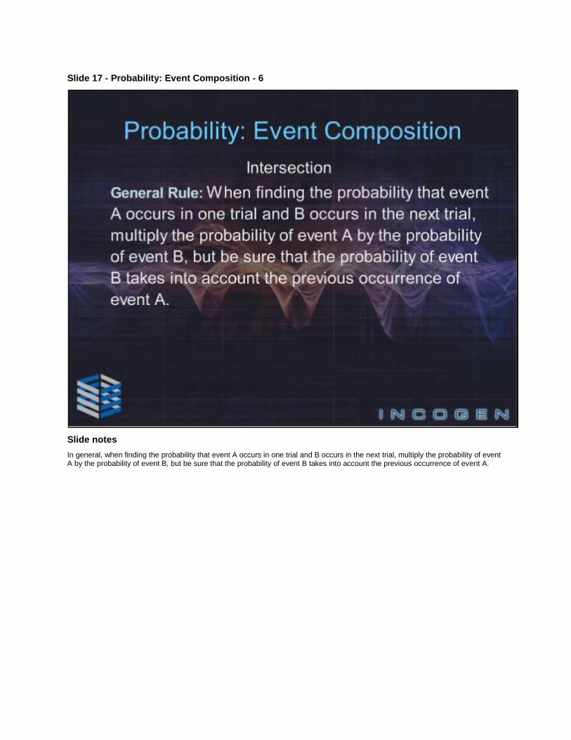
Slide notes In general, when finding the probability that event A occurs in one trial and B occurs in the next trial, multiply the probability of event A by the probability of event B, but be sure that the probability of event B takes into account the previous occurrence of event A.

Slide 18 - Probability: Event Composition-7

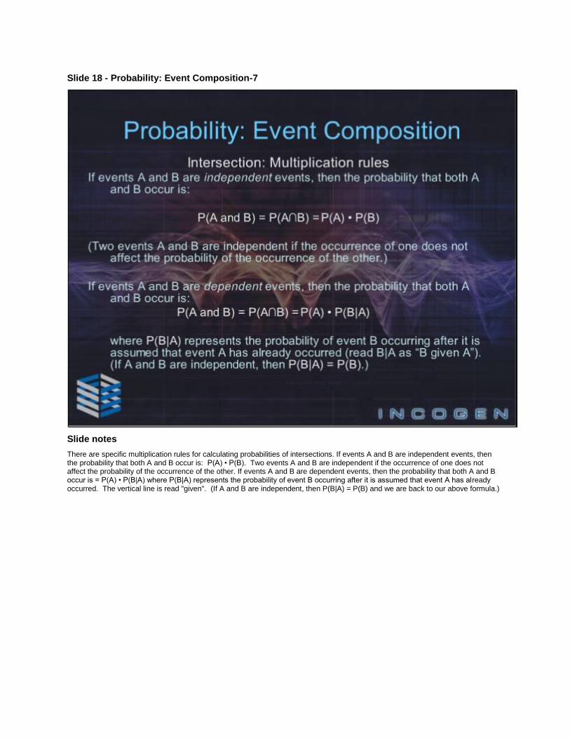
Slide notes There are specific multiplication rules for calculating probabilities of intersections. If events A and B are independent events, then the probability that both A and B occur is: P(A) • P(B). Two events A and B are independent if the occurrence of one does not affect the probability of the occurrence of the other. If events A and B are dependent events, then the probability that both A and B occur is = P(A) • P(B|A) where P(B|A) represents the probability of event B occurring after it is assumed that event A has already occurred. The vertical line is read "given". (If A and B are independent, then P(B|A) = P(B) and we are back to our above formula.)

Slide 19 - Probability: Event Composition-8

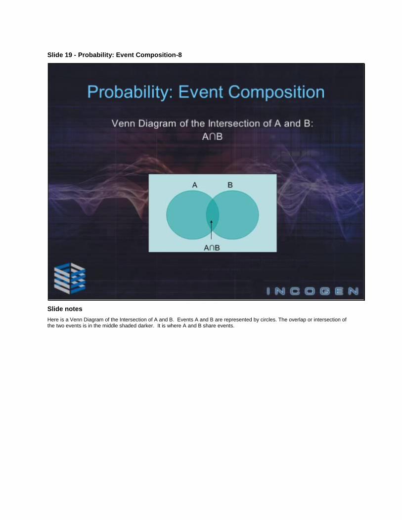
Slide notes Here is a Venn Diagram of the Intersection of A and B. Events A and B are represented by circles. The overlap or intersection of the two events is in the middle shaded darker. It is where A and B share events.

Slide 20 - Simple Probability Example Continued 3

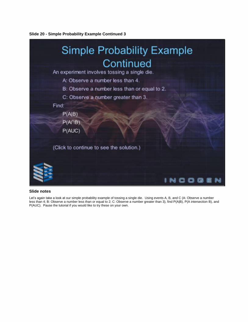
Slide notes Let’s again take a look at our simple probability example of tossing a single die. Using events A, B, and C (A: Observe a number less than 4; B: Observe a number less than or equal to 2; C: Observe a number greater than 3), find P(A|B), P(A intersection B), and P(AUC). Pause the tutorial if you would like to try these on your own.

Slide 21 - Simple Probability Example Continued -4

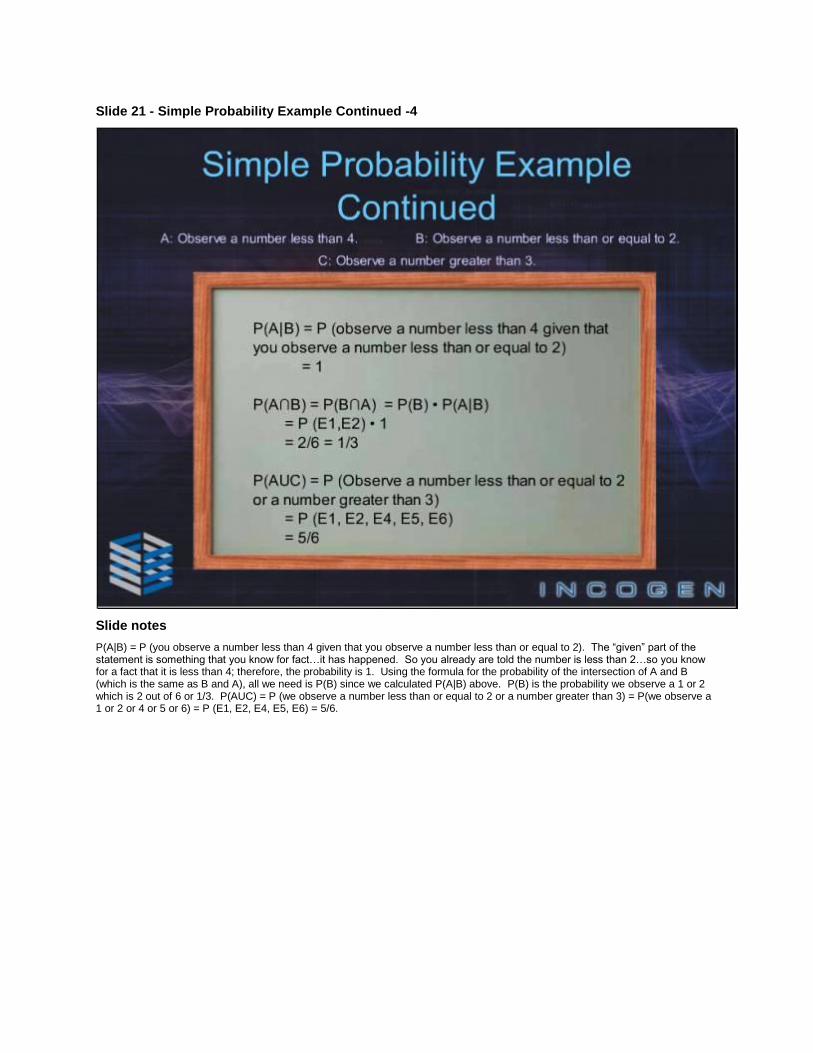
Slide notes P(A|B) = P (you observe a number less than 4 given that you observe a number less than or equal to 2). The “given” part of the statement is something that you know for fact…it has happened. So you already are told the number is less than 2…so you know for a fact that it is less than 4; therefore, the probability is 1. Using the formula for the probability of the intersection of A and B (which is the same as B and A), all we need is P(B) since we calculated P(A|B) above. P(B) is the probability we observe a 1 or 2 which is 2 out of 6 or 1/3. P(AUC) = P (we observe a number less than or equal to 2 or a number greater than 3) = P(we observe a 1 or 2 or 4 or 5 or 6) = P (E1, E2, E4, E5, E6) = 5/6.

Slide 22 - Random Variables

Slide notes For our last topic, probability distributions, we need to define random variables. A random variable x is a variable that has a single numerical value, determined by chance, for each outcome of an experiment. In our simple example of rolling a die, x can equal a 1, 2, 3, 4, 5, or 6.

Slide 23 - Probability Distributions

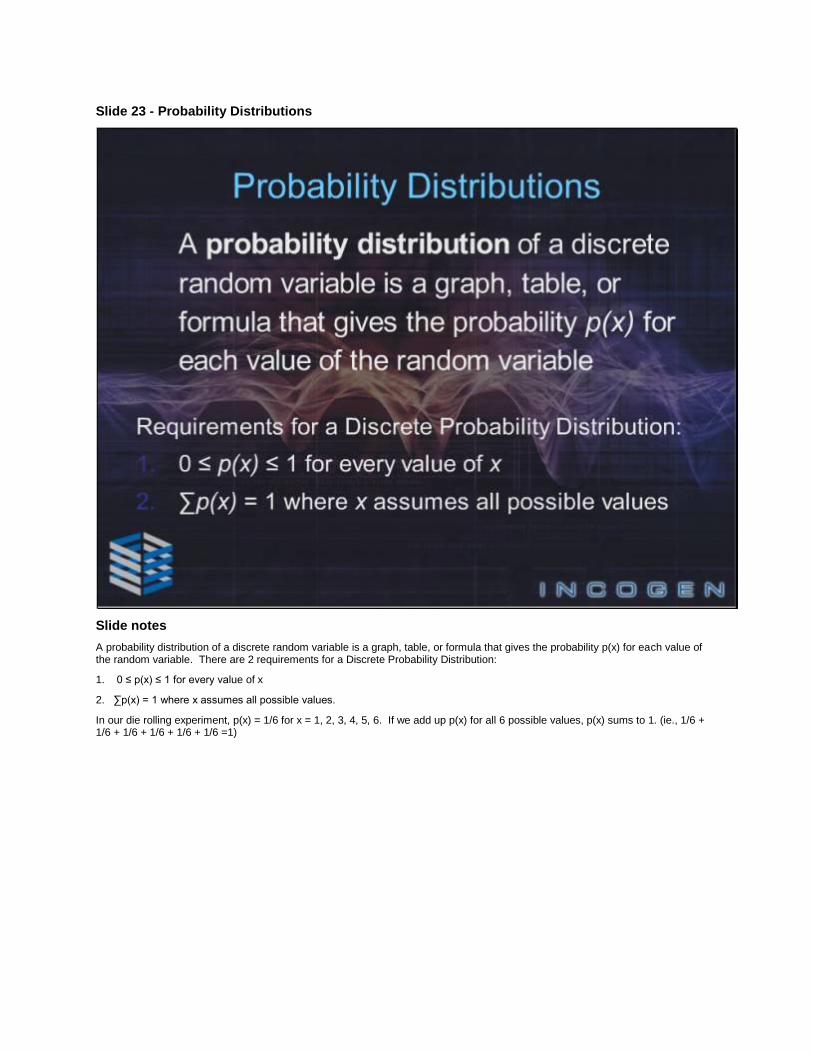
Slide notes A probability distribution of a discrete random variable is a graph, table, or formula that gives the probability p(x) for each value of the random variable. There are 2 requirements for a Discrete Probability Distribution: 1. 0 ≤ p(x) ≤ 1 for every value of x 2. ∑p(x) = 1 where x assumes all possible values. In our die rolling experiment, p(x) = 1/6 for x = 1, 2, 3, 4, 5, 6. If we add up p(x) for all 6 possible values, p(x) sums to 1. (ie., 1/6 + 1/6 + 1/6 + 1/6 + 1/6 + 1/6 =1)

Slide 24 - Probability Distribution

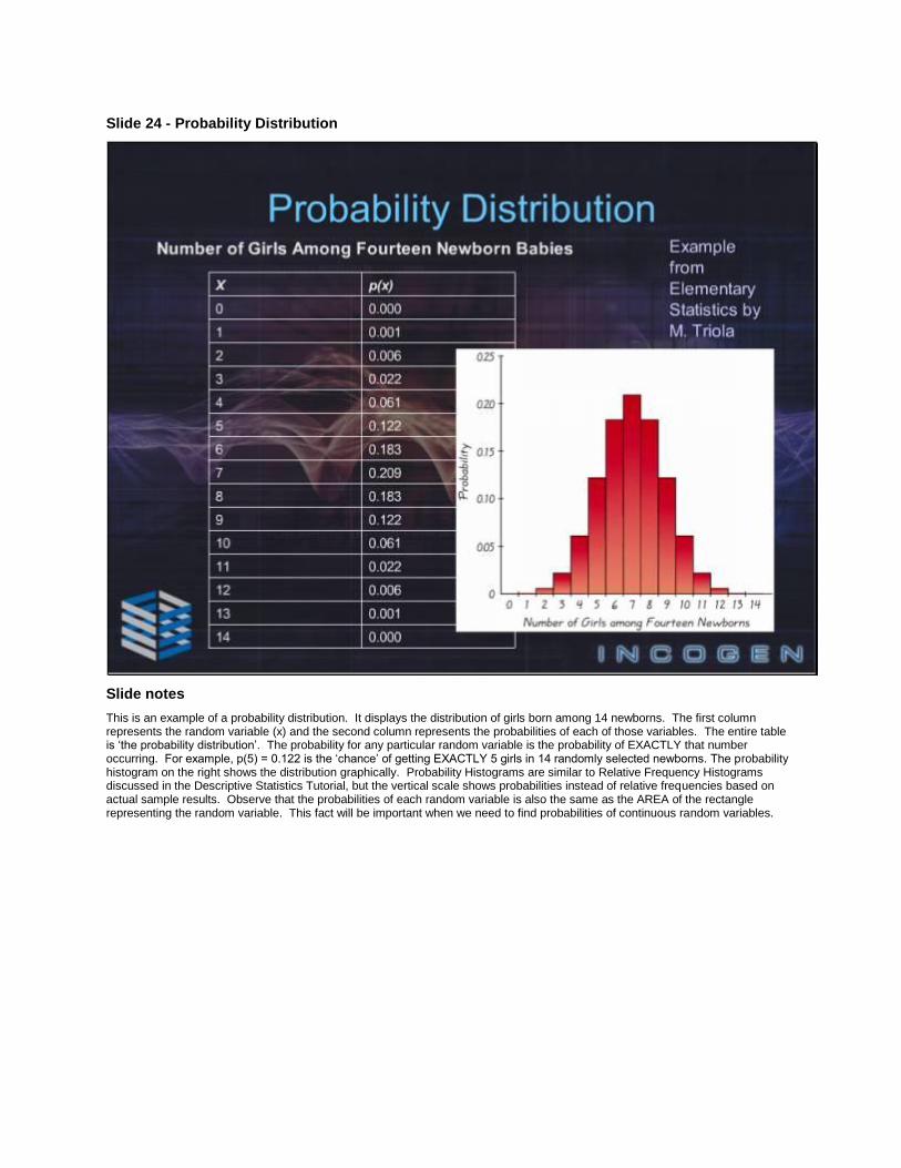
Slide notes This is an example of a probability distribution. It displays the distribution of girls born among 14 newborns. The first column represents the random variable (x) and the second column represents the probabilities of each of those variables. The entire table is ‘the probability distribution’. The probability for any particular random variable is the probability of EXACTLY that number occurring. For example, p(5) = 0.122 is the ‘chance’ of getting EXACTLY 5 girls in 14 randomly selected newborns. The probability histogram on the right shows the distribution graphically. Probability Histograms are similar to Relative Frequency Histograms discussed in the Descriptive Statistics Tutorial, but the vertical scale shows probabilities instead of relative frequencies based on actual sample results. Observe that the probabilities of each random variable is also the same as the AREA of the rectangle representing the random variable. This fact will be important when we need to find probabilities of continuous random variables.

Slide 25 - Numerical Descriptive Measures for Discrete Random Variables: Mean, Variance and Standard Deviation

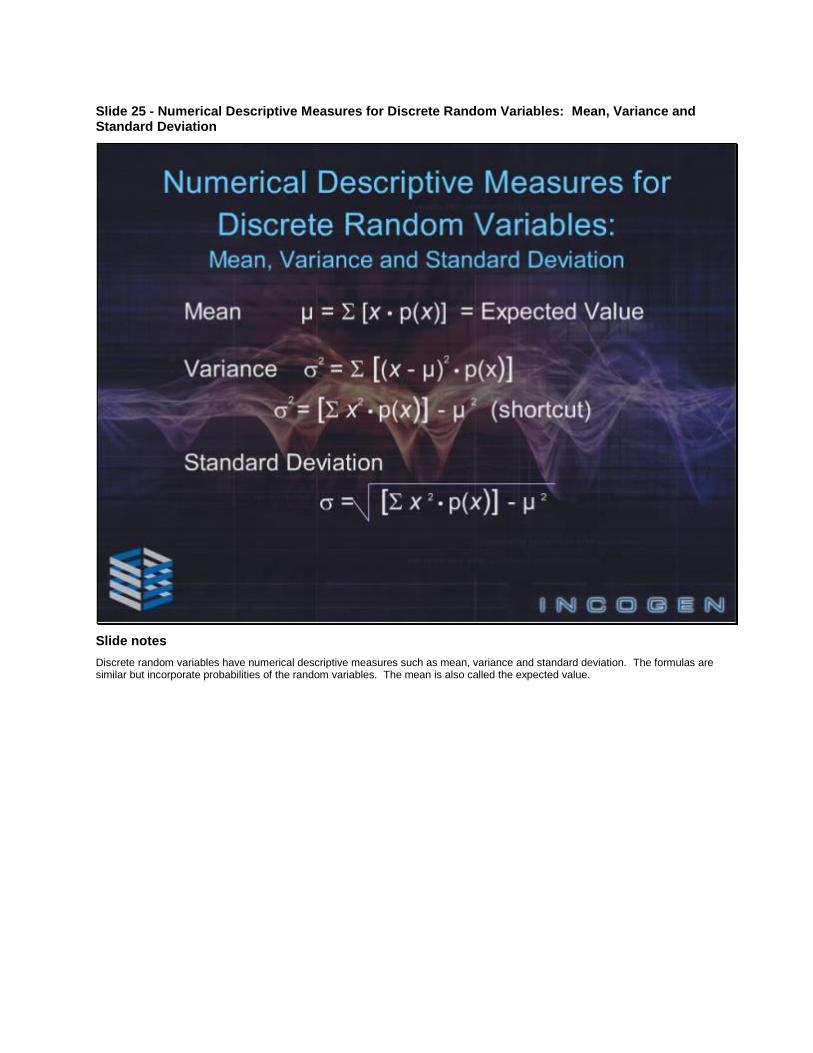
Slide notes Discrete random variables have numerical descriptive measures such as mean, variance and standard deviation. The formulas are similar but incorporate probabilities of the random variables. The mean is also called the expected value.

Slide 26 - Mean, Variance and Standard Deviation for our Newborn Example

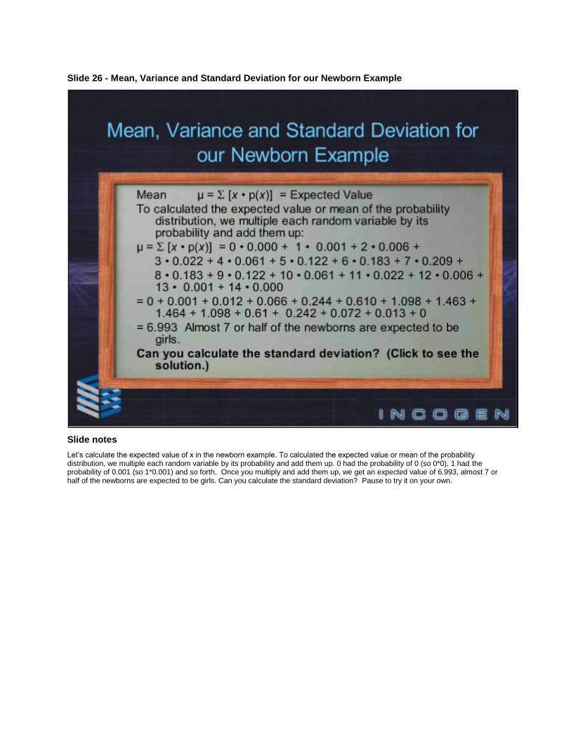
Slide notes Let’s calculate the expected value of x in the newborn example. To calculated the expected value or mean of the probability distribution, we multiple each random variable by its probability and add them up. 0 had the probability of 0 (so 0*0), 1 had the probability of 0.001 (so 1*0.001) and so forth. Once you multiply and add them up, we get an expected value of 6.993, almost 7 or half of the newborns are expected to be girls. Can you calculate the standard deviation? Pause to try it on your own.

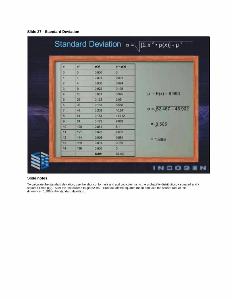
Slide 27 - Standard Deviation

Slide notes To calculate the standard deviation, use the shortcut formula and add two columns to the probability distribution, x squared and x squared times p(x). Sum the last column to get 52.467. Subtract off the squared mean and take the square root of the difference. 1.888 is the standard deviation.

Slide 28 - References

Slide notes This concludes part 1 of our tutorial on probability and probability distributions. This material and more details can be found in the listed resources.